Time series data are intriguing yet complicated information to work with. While this Credits 3 course will provide students with a basic understanding of the nature and basic processes used to analyze such data, you will quickly realize that this is a small first step in being able to confidently understand what trends might exist within a set of data and the complexities of being able to use this information to make predictions or forecasts. Yet, whether it is financial, medical or weather related, this type of data is quite frequently found in much of our daily lives.
PREREQUISITES
Topics typically covered in this graduate level course include:
Understanding the characteristics of time series data
Understanding moving average models and partial autocorrelation as foundations for analysis of time series data
Exploratory Data Analysis – Trends in time series data
Using smoothing and removing trends when working with time series data
Understanding how periodograms are used with time series data
Implementing ARMA and ARIMA time series models
Identifying and interpreting various patterns for intervention effects
Examining the analysis of repeated measures design
Using ARCH and AR models in multivariate time series contexts
Using spectral density estimation and spectral analysis
Using fractional differencing and threshold models with time series data
2.5 Find the command for graphing quarterly seasonal plots in the Python package statsmodels, and then graph the seasonal plots for the dataset in Example 2.6 as well as give your comment on the plot.
问题 2.
2.6 Use the multiplicative Holt-Winters smoothing method to analyze the dataset “gdpquarterlychina1992.1-2017.4.csv,” and compare your results with the results in Example 2.6
问题 3.
2.7 The time series data “AustraliaUnemployedTotalPersons” in the folder “Ptsadata” is from the Australian Bureau of Statistics. Make an exploratory data analysis of it.
问题 4.
2.8 For the interpretation of economic statistics such as unemployment data or GDP data, it is important to identify the presence of seasonal components and to remove them so as to eliminate the effect of seasonal influence on the raw time series and reveal the true trend. This process is called the seasonal adjustment, and if the seasonal components are removed from the original time series data, the resulting values are known as the seasonally adjusted time series. Using the seasonal decompose function, make a seasonal adjustment of the time series data “gdpquarterlychina1992.1-2017.4.csv,” and describe what is the difference between the seasonally adjusted series and the trend component.
Textbooks
• An Introduction to Stochastic Modeling, Fourth Edition by Pinsky and Karlin (freely available through the university library here) • Essentials of Stochastic Processes, Third Edition by Durrett (freely available through the university library here) To reiterate, the textbooks are freely available through the university library. Note that you must be connected to the university Wi-Fi or VPN to access the ebooks from the library links. Furthermore, the library links take some time to populate, so do not be alarmed if the webpage looks bare for a few seconds.
统计代写|时间序列分析代写Time-Series Analysis代考|Properties of ARMA Models
Pertaining to the stationarity, invertibility, and causality, the following theorem is not hard to understand.
Theorem 3.3 (1) The $\operatorname{ARMA}(p, q)$ is stationary if and only if its AR part is stationary. (2) The $\operatorname{ARMA}(p, q)$ is invertible if and only if its MA part is invertible. (3) The $A R M A(p, q)$ is causal if and only if its AR part is causal. For the coefficients $\left{\pi_j\right}$ in the $\operatorname{AR}(\infty)$ representation and the coefficients $\left{\psi_j\right}$ in the $\mathrm{MA}(\infty)$ representation, it is easy to prove the following propositions.
If an $\operatorname{ARMA}(p, q)$ model defined by (3.7) is invertible, then its $\operatorname{AR}(\infty)$ representation is $$ \varepsilon_t=\sum_{j=0}^{\infty} \pi_j X_{t-j}=\left(\sum_{j=0}^{\infty} \pi_j B^j\right) X_t $$ where $\pi_0=1$ and for $j \geq 1$ $$ \pi_j=-\sum_{k=1}^j \theta_k \pi_{j-k}-\varphi_j \text { where } \theta_k=0 \text { for } k>q, \varphi_j=0 \text { for } j>p . $$
If an $\operatorname{ARMA}(p, q)$ model defined by (3.7) is causal, then its $\operatorname{MA}(\infty)$ representation is $$ X_t=\sum_{j=0}^{\infty} \psi_j \varepsilon_{t-j}=\left(\sum_{j=0}^{\infty} \psi_j B^j\right) \varepsilon_t $$ where $\psi_0=1$ and for $j \geq 1$ $$ \psi_j=\sum_{k=1}^j \varphi_k \psi_{j-k}+\theta_j \text { where } \varphi_k=0 \text { for } k>p, \theta_j=0 \text { for } j>q . $$
统计代写|时间序列分析代写Time-Series Analysis代考|Model Building Problems
For building an ARMA model, a time series dataset is required to be stationary. Thus before estimating the ARMA model, we should check if the time series data is stationary using those procedures in Sect. 3.1.
In Chap. 3, we have given the definition of the ARMA model and elaborated on its properties. Now we know that Eq. (3.7) is the $\operatorname{ARMA}(p, q)$ model: $$ X_t=\varphi_0+\varphi_1 X_{t-1}+\cdots+\varphi_p X_{t-p}+\varepsilon_t+\theta_1 \varepsilon_{t-1}+\cdots+\theta_q \varepsilon_{t-q} $$ where $\left{\varepsilon_t\right} \sim \mathrm{WN}\left(0, \sigma_\epsilon^2\right), \varphi_p \neq 0, \theta_q \neq 0$ and $\varphi_0$ is the intercept (const). Another expression of the $\operatorname{ARMA}(p, q)$ model is $$ \varphi(B) X_t=\varphi_0+\theta(B) \varepsilon_t $$ where $\varphi(z)=1-\varphi_1 z-\cdots-\varphi_p z^p, \theta(z)=1+\theta_1 z+\cdots+\theta_q z^q$. Hence the number of parameters to be estimated is $p+q+2$. Additionally, in practice, $\operatorname{order}(p, q)$ is also unknown and needs to be determined.
There are two important procedures for selecting ARMA model order $(p, q)$. One is to firstly compute ACF as well as PACF and then by Table 3.1 to choose $\operatorname{order}(p, q)$. Another is a few information criteria such as AIC, BIC, HQIC, and so on. We will present these methods in detail in Sect. 4.3.
If $X_t$ has no seasonality and by differencing, we have that $Y_t=\nabla^d X_t=(1-$ $B)^d X_t$ is stationary (sometimes we need firstly transform the original series), then we can build an $\operatorname{ARMA}(p, q)$ model for $Y_t$ as follows: $$ \varphi(B) Y_t=\varphi_0+\theta(B) \varepsilon_t . $$ Expressing this model in terms of the original time series $X_t$, we have $$ \varphi(B)(1-B)^d X_t=\varphi_0+\theta(B) \varepsilon_t . $$
统计代写|时间序列分析代写Time-Series Analysis代考|Stationarity and Causality of AR Models
Consider the AR(1) model: $$ X_t=\varphi X_{t-1}+\varepsilon_t, \varepsilon_t \sim \mathrm{WN}\left(0, \sigma_\epsilon^2\right) $$ For $|\varphi|<1$, let $X_{1 t}=\sum_{j=0}^{\infty} \varphi^j \varepsilon_{t-j}$ and for $|\varphi|>1$, let $X_{2 t}=-\sum_{j=1}^{\infty} \varphi^{-j} \varepsilon_{t+j}$. It is easy to show that both $\left{X_{1 t}\right}$ and $\left{X_{2 t}\right}$ are stationary and satisfy Eq. (3.6). That is, both are the stationary solution of Eq. (3.6). This gives rise to a question: which one of both is preferable? Obviously, $\left{X_{2 t}\right}$ depends on future values of unobservable $\left{\varepsilon_t\right}$, and so it is unnatural. Hence we take $\left{X_{1 t}\right}$ and abandon $\left{X_{2 t}\right}$. In other words, we require that the coefficient $\varphi$ in Eq. (3.6) is less 1 in absolute value. At this point, the AR(1) model is said to be causal and its causal expression is $X_t=\sum_{j=0}^{\infty} \varphi^j \varepsilon_{t-j}$. In general, the definition of causality is given below.
Definition 3.7 (1) A time series $\left{X_t\right}$ is causal if there exist coefficients $\psi_j$ such that $$ X_t=\sum_{j=0}^{\infty} \psi_j \varepsilon_{t-j}, \sum_{j=0}^{\infty}\left|\psi_j\right|<\infty $$ where $\psi_0=1,\left{\varepsilon_t\right} \sim \operatorname{WN}\left(0, \sigma_\epsilon^2\right)$. At this point, we say that the time series $\left{X_t\right}$ has an $\mathrm{MA}(\infty)$ representation. (2) We say that a model is causal if the time series generated by it is causal.
Causality suggests that the time series $\left{X_t\right}$ is caused by the white noise (or innovations) from the past up to time $t$. Besides, the time series $\left{X_{2 t}\right}$ is an example that is stationary but not causal. In order to determine whether an AR model is causal, similar to the invertibility for the MA model, we have the following theorem.
统计代写|时间序列分析代写Time-Series Analysis代考|Autoregressive Moving Average Models
Now we give the definition of ARMA models as follows. Definition 3.8 (1) The following equation is called the autoregressive moving average model of order $(p, q)$ and denoted by $\operatorname{ARMA}(p, q)$ : $$ X_t=\varphi_0+\varphi_1 X_{t-1}+\cdots+\varphi_p X_{t-p}+\varepsilon_t+\theta_1 \varepsilon_{t-1}+\cdots+\theta_q \varepsilon_{t-q} $$ where $\left{\varepsilon_t\right} \sim \mathrm{WN}\left(0, \sigma_\epsilon^2\right), \mathrm{E}\left(X_s \varepsilon_t\right)=0$ if $s<t$, and $\left{\varphi_k\right}$ and $\left{\theta_k\right}$ are real-valued parameters (coefficients) with $\varphi_p \neq 0$ and $\theta_q \neq 0$. (2) If a time series $\left{X_t\right}$ is stationary and satisfies such an equation as (3.7), then we call it an $\operatorname{ARMA}(p, q)$ process.
We often assume the intercept (const term) $\varphi_0=0$. Using the backshift operator $B$, the $\operatorname{ARMA}(p, q)$ model can be rewritten as $$ \varphi(B) X_t=\theta(B) \varepsilon_t $$ where $\varphi(z)=1-\varphi_1 z-\cdots-\varphi_p z^p$ is the AR polynomial and $\theta(z)=1+\theta_1 z+$ $\cdots+\theta_q z^q$ is the MA polynomial. We always assume that $\varphi(z)$ and $\theta(z)$ have no common factors. Besides, $\varphi(B) X_t=\varepsilon_t$ and $X_t=\theta(B) \varepsilon_t$ are, respectively, called the $A R$ part and $M A$ part of the ARMA $(p, q)$ model. Of course, both the AR model and MA model are two special cases of the $\operatorname{ARMA}$ model: $\operatorname{AR}(p)=\operatorname{ARMA}(p, 0)$ and $\operatorname{MA}(q)=\operatorname{ARMA}(0, q)$
Example 3.11 (An ARMA(2,2) Model) Consider the following ARMA(2,2) model: $$ X_t=0.8 X_{t-1}-0.6 X_{t-2}+\varepsilon_t+0.7 \varepsilon_{t-1}+0.4 \varepsilon_{t-2} $$ We can simulate it with Python. Its time series plot is shown in Fig. 3.19 and looks stationary. In addition, its ACF and PACF plots are shown in Fig. 3.20. Both ACF and PACF seem to tail off, namely, for lag $k \geq 3$, and many ACF and PACF values are still nonzero. The Python code for this example is as follows.
统计代写|时间序列分析代写Time-Series Analysis代考|Introduction and Installing
Python is an interpreted high-level language for general-purpose programming. It was first created by Mr. Guido van Rossum from the Netherlands (now he lives in the United States) and released for people to free use in 1991. Presently it is run by the Python Software Foundation, which is a non-profit organization created specifically to own Python-related Intellectual Property. Python has a simple but effective approach to object-oriented programming and design philosophy that emphasizes code readability, notably using significant whitespace. It provides architecture that enables clearly programming on both small and large scales. It has a large and comprehensive standard library that supports many common programming tasks such as connecting to web servers, searching text with regular expressions, and reading and modifying files. It is easily extended by adding new modules implemented in a compiled language such as $\mathrm{C}$ or $\mathrm{C}++$. Python has a variety of basic data types available: numbers (floating point, complex, and unlimited-length long integers), strings (both ASCII and Unicode), lists, and dictionaries. It also supports raising and catching exceptions, resulting in cleaner error handling. Python’s automatic memory management frees you from having to manually allocate and free memory in your code. In recent years, Python has been continuing to take leading positions in solving big data science tasks and artificial intelligence challenges.
The Python interpreter and the standard library are freely available in source or binary form for all major operational systems (OS) from the Python website: https://www.python.org/. According to the OS of your computer, you can download the corresponding Python interpreter to your computer and easily install it. Since the standard library is distributed with the Python interpreter, it is installed together with Python. In this book, we install Python-3.6.5-amd64 for Windows 10, and all the codes are run on this version of Python. We do not intend to totally introduce the Python syntax and semantics about which you can refer to the documentations in the Python website and related books. We only demonstrate some usages of Python, which are often used in the book. At present, there are many so-called enhanced or integrated versions of Python. If you are a new learner, we do not recommend any of them because using the plain Python, we can better understand it. If you have some experience with Python, you can use any of Python distributions that you are used to. And Anaconda is perhaps your favorite platform.
统计代写|时间序列分析代写Time-Series Analysis代考|Python Extension Packages and Some Usages
There are a large number of the third-party Python extension packages, which are applied in various fields. In this subsection, we introduce a few of them. They are very useful in scientific computing, statistical analysis, data visualization, and so on. First of all, we recommend that you use pip to install and manage Python extension packages. Starting with Python 3.4 , it is included with the Python installer by default and so has already been installed. Clicking the start menu with the right mouse button, we will see the Windows PowerShell (Administrator) menu. Opening it, we get a prompt like this:
If you want to install an extension package from the network, type and run the following command: PS C: \WINDOWS $\backslash$ system32> pip install packagename Here pip is a Python package installing and managing tool. As long as the network that you are using is well unobstructed, in general, the installation will be successful. If you have downloaded and stored a package (e.g., the package pandas) in your computer, then you can run the command below to install it: PS C: \WINDOWS \system32> pip install $\mathrm{J}$ : \extension $\backslash$ pandas- 0.23 .4 -cp36-cp36m-win_amd64.whl # “J: \extension $\backslash$ pandas-0.23.4-cp36-cp36m-win_amd64.wh̄l” $#$ is the path and name for pandas The following is the five Python extension packages that we have installed:
Numpy (version 1.15.4) is a fundamental and general-purpose array-processing package designed to manipulate large multi-dimensional arrays of arbitrary records (such as numbers, strings, objects, and others). It also includes tools for integrating $\mathrm{C} / \mathrm{C}++$ and Fortran code; random number generators; discrete Fourier transform; and so forth. Besides, Numpy can also be used as an efficient multidimensional container of generic data. It possesses the ability to define arbitrary data types. This allows it to seamlessly and speedily integrate with a wide variety of databases. Its homepage is https://www.numpy.org/.
统计代写|时间序列分析代写Time-Series Analysis代考|The Concept of Time Series
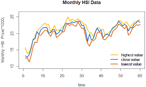
It is a big data era nowadays. The world is full of various kinds of data. And time series are one of the most common data type. There is a great deal of time series data in both everyday life and fields of sciences and technology. However, what is a time series? Roughly speaking, the time series is a sequence of data from a natural or social process (or a trial) observed over time. So it is “time” ordered, and we must not interchange the positions of any two values of the time series. There are a lot of time series examples in our everyday life. For instance, your body weight measured on every Sunday forms a time series; the daily closing price of a listed company stock also shapes a time series. The first step in any time series analysis is always to plot the recorded time series data and carefully examine this graph. In a coordinate system, let the index of time $t$ be on the horizontal axis and the observed value on the vertical axis. Thus the time series data are plotted against time. Such a graph is known as a time series plot or time plot. It is easy to plot but very useful in analyzing time series. It displays the evolution pattern of a time series. The pattern includes the trend and/or seasonality (period) of the time series. Below are a few examples of time series.
Example 1.1 (Bitcoin Price Time Series) In recent years, digital currencies are hot and Bitcoin is the most famous. From June 23, 2017, to June 22, 2018, the Bitcoin price was recorded at the end of every day, and the recorded data forms the Bitcoin price time series. Now we can use Python to plot it (in the next sections, we will learn how to plot it with Python). Figure 1.1 is the Bitcoin price time series plot. From the plot, we observe that the Bitcoin price dramatically increases from October 2017 and reaches the peak at the end of 2017 (actually, the peak is 19187.0 USD reached in December 16, 2017). And since then, the price fluctuantly decreases. This time series plot clearly reflects some people’s craziness about Bitcoin. ${ }^1$
统计代写|时间序列分析代写Time-Series Analysis代考|Brief History of Time Series Analysis
As early as 28 BC during the Western Han Dynasty in China, there exists the recording of sunspots (e.g., see Needham (1959) and Tong (1990)). Nowadays we can obtain the annual mean total sunspot number from 1700 to 2017 from the Royal Observatory of Belgium, Brussels. It forms a time series of length 318 years. Figure 1.4 is its time series plot, and we see that there is a some kind of period but no trend in it. In other words, the evolution pattern of the sunspot number time series has hardly changed since 1700 .
The theoretical developments in time series analysis started in the 1920 s and 1930 s when the strict basics of probability theory was being constructed by the Russian mathematician A. N. Kolmogorov. During that time, the Russian statistician E. Slutsky and the British statisticians G. U. Yule and J. Walker introduced MA (moving average) models and AR (autoregressive) models to represent time series and used the moving average method to remove seasonal effect in a time series. See, for example, Slutsky (1927) and Yule (1927). And then H. Wold developed ARMA (autoregressive moving average) models for stationary time series. In 1970, the classic book Time Series Analysis: Forecasting and Control by G. E. P. Box and G. M. Jenkins was published, which contains the full modeling procedure for a (maybe nonstationary) time series: identification, estimation, diagnostics, and forecasting. ${ }^2$ Today, the Box-Jenkins models (or procedure) are perhaps the most commonly used, and many methods for forecasting and seasonal adjustment can be traced back to these models.
One direction of continuing development in time series analysis is multivariate ARMA models, among which VAR (vector autoregressive) models have especially become popular. The pity is that these techniques are only applicable for stationary time series. However, real-life time series often possess an ascending trend which suggests nonstationarity (viz., a unit root). In the 1980s and 1990s, a few of important tests for unit roots developed. On the other hand, it was found that nonstationary multivariate time series could have a common unit root. These time series are known as cointegrated time series and can be used in the error correction models where both long-term relationships and short-term dynamic mechanism are estimated.
统计代写|时间序列分析代写Time-Series Analysis代考|Prediction, Classification, and Chaos
The attractor of the dynamical systems producing $s(t)$ is contained in dimension $d_E$ which assures that there is no residual overlap of trajectories from the projection to one dimension: $s(t)$. To characterize the attractor we can call on many different notions of dimension of the set of points $\mathbf{y}(\mathrm{n})$. Each is an invariant of the dynamical system in the sense that a smooth coordinate change from those used in $y(n)$, including that involved in changing $T$, leaves these characteristic numbers unchanged. The invariance comes from the fact that each dimension estimate is a local property of the point set comprising the attractor, and smooth changes of coordinates do not alter this local property while they might change the global appearance of the attractor. These various dimensions are covered in many books, and each is interesting.
We here focus on a dynamical invariant of the attractor that also allows an estimate of dimension. The central issue is the stability of an orbit such as $\mathbf{y}(\mathrm{n})$ under perturbations to points on the trajectory. This is a familiar question associated with the stability of fixed points or limit cycles as studied in classical fields such as fluid dynamics. If one has a fixed point $x_0$ of a dynamical system in d dimension $x(t)=\left[x_1(t), x_2(t), \ldots, x_d(t)\right]$ with $x(t)$ satisfying $$ \frac{d x(t)}{d t}=\mathbf{G}(x(t)) $$ so $\mathbf{G}\left(\mathrm{x}_0\right)=0$, then it is important to ask if state space points $x_0+\Delta x(t)$ are stable in the sense they remain near or return to $x_0$. Unstable points, where $\Delta x(t)$ grows large, are not realized in observations of a dynamical system.
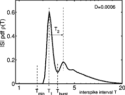
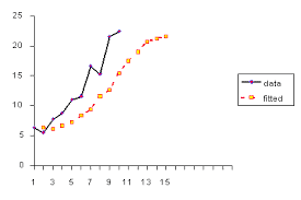
To start with a simple example for black-box modeling we consider the interspike intervals of the given neuron time series shown in Fig. 2.8. As already mentioned in Section 2.2.3 this diagram suggests an approximate description in terms of some function $\Delta t_{k+1}=g\left(\Delta t_k\right)$. The goal of (black-box) modeling is to find a function $g$ that fulfills this task in some optimal sense (to be specified). In particular, the function should have good generalization properties: not only the given time series has to be mapped correctly but also new data from the same source (not yet seen when learning the model). To achieve this (ambitious) goal overfitting has to be avoided, i.e., the model must not incorporate features of the particular realization of the given (finite!) time series. The performance of a good model does not depend on statistical features like random choice of initial conditions on a (chaotic) attractor or purely stochastic components (noise) that will not be the same for different measurements from a fixed (stationary) source or process. So the model has to be flexible enough to describe the data but should not be too complex, because then it will start to model also realization-dependent features. To determine some suitable level of complexity one may employ complexity measures and balance them with the prediction error. Another practically useful method is cross validation. The given data set is split into two parts: a learning or training set and an independent test set. The training set is used to specify the model (including parameters), and this model is then applied to the test set to evaluated its generalization properties and potential overfitting. To illustrate this point we shall fit a polynomial to the interspike intervals within a burst shown in Fig. $2.8$ (enlargement on the right-hand side). These data points are randomly split into two halves, training and test set. A polynomial of degree $m$ is fit to the training set and then used to map the test data points. For both sets of points mean squared errors are computed, called $E_{\text {train }}$ and $E_{\text {test. }}$ In Fig. $2.12$ both errors are plotted versus $m$. Increasing the degree $m$ renders our model more complex and results in a monotonically decreasing error $E_{\text {train }}$ of the training set (dashed line in Fig. 2.12). For small $m$ the error $E_{\text {test }}$ of the test set also decreases but at $m=3$ it starts to increase again, because for too complex polynomials overfitting sets in and the performance of the model on the test set deteriorates. To obtain a representative and robust evaluation of the model performance the time series has been split randomly several times in different training and test sets and the given errors are mean values of the corresponding training and test errors.
The next question about the data vector $$ \mathbf{y}(n)=[s(n), s(n-T), \ldots, s(n-(D-1) T)] $$ we need to address is the value of the integer “embedding dimension” D. Here is where Whitney’s and Takens’ results come into play. The key idea is that as we enlarge the dimension $D$ of the vector $\mathbf{y}(n)$ we eliminate step by step the intersections of orbits on the system attractor arising from our projection during the measurement process. If this is the case, then there might well be a global dimension allowing us to unfold a particular data set with particular coordinates as entries in $\mathbf{y}(n)$ at a dimension less than the sufficient dimension of the Whitney/Takens geometric result.
To examine this we need the notion of crossing of trajectories, and this we realize in the close analogy of neighbors in the state space which are a result of the dynamics-true neighbors-and neighbors in the state space which are a result of the projection during measurement-false neighbors [23]. If we select an embedding dimension $\mathrm{D}$, then it is a matter of an $\operatorname{order} \mathrm{N} \log (\mathrm{N})$ search among all the points $\mathbf{y}(n)$ in that space to determine the nearest neighbor to a point $\mathbf{y}(\mathrm{k})$. If this nearest neighbor is not a close neighbor in dimension $\mathrm{D}+1$, then its “neighborliness” to $\mathbf{y}(\mathrm{k})$ is the result of a projection from a higher dimensional space. This is a false nearest neighbor, and we wish to eliminate all of them. We accomplish this elimination of the false nearest neighbors by systematically examining the nearest neighbors in dimension $\mathrm{D}$ and their “neighborliness” in dimension D $+1$ for $\mathrm{D}=1,2, \ldots$ until there are no false nearest neighbors remaining. We call this integer dimension $d_E$.
统计代写|时间序列分析代写Time-Series Analysis代考|Local or Dynamical Dimension
The embedding dimension we just selected is a global and average indicator of the number of coordinates needed to unfold the actual data $s(t)$ [24].
The global integer embedding dimension estimate tells us a minimum dimension $d_E$ in which we can place (embed) the signal from our source. This dimension can be larger than the number of degrees of freedom in the dynamics underlying the signal $s(t)$. Suppose that locally the dynamics happened to be a two-dimensional map $\left(x_n, y_n\right) \rightarrow\left(x_{n+1}, y_{n+1}\right)$ but the global structure of the dynamics placed this on the surface of an ordinary torus. To embed the points of the whole data set now lying on a torus, we would have to select $d_E=3$; however, if we wish to determine equations of motion (or a map) to describe the dynamics, we really need only the local dimension of 2 . This local dimension $d_L \leqslant d_E$, and is important when we wish to evaluate the Lyapunov exponent, as we do below, to characterize the dynamical system producing $s(t)$.
To determine $d_L$ we need to move beyond the geometry in the embedding theorem and ask a local question about the data in dimension $\mathrm{d}{\mathrm{E}}$ where we know there are no unwanted intersections of the orbit associated with $s(t)$ and itself. The notion is that data vectors of dimension $\mathrm{d} \leqslant \mathrm{d}{\mathrm{E}}$, $$ y_d(n)=[s(n), s(n-T), \ldots, s(n-(d-1) T)], $$ will map without ambiguity locally into other vectors of dimension $d \leqslant d_E$. We can test for this by forming a d-dimensional local map $$ \mathbf{y}{\mathrm{d}}(\mathrm{n}+1)=\mathbf{M}\left(\mathbf{y}{\mathrm{d}}(\mathrm{n})\right), $$ and asking whether this map accounts for the behavior of the actual data in $\mathrm{d} \leqslant \mathrm{d}{\mathrm{E}}$. For $\mathrm{d}$ too small, it will not. For $\mathrm{d}=\mathrm{d}{\mathrm{E}}$, it will. If for some intermediate $\mathrm{d}$, the map is accurate, this is an indication of a lower dimensional dynamics than $\mathrm{d}_{\mathrm{E}}$ needed to globally unfold the data.
To answer this question select a data vector $y(k)$ in $d_E$. Select $N_B$ nearest neighbors in phase space to $y(k): y^{(r)}(k) ; r=0,1,2, \ldots, N_B, y^{(0)}(k)=y(k)$. In $\mathrm{d}{\mathrm{E}}$ these are all true neighbors, but their actual time labels may or may not be near the time k. Choose in various ways a d-dimensional subspace of vectors $\mathbf{y}{\mathrm{d}}^{(r)}(\mathrm{k})$. There are $\left(\begin{array}{c}\mathrm{d}_{\mathrm{E}} \ \mathrm{d}\end{array}\right)$ ways to do this and all are worth examining.
统计代写|时间序列分析代写Time-Series Analysis代考|Unfolding the Data: Embedding Theorem in Practice
We will primarily focus on the usual and simplest case of time series measurements of a single signal $s(t)$. If more than a single measurement is available, there are additional questions one may ask and answer. The signal is observed with some accuracy, usually specified by an estimate of the “noise” level associated with interference of the measurement by other processes. The signal is also measured in discrete time, starting at an initial time $t_0$ and then typically at a uniform time interval $\tau_s$ we call the sampling time. $s(t)$ is thus the set of $N$ measurements $s\left(t_0+n \tau_s\right), n=1,2, \ldots, N$.
The dynamical system from which the signal comes is usually unknown in detail. In the case of the LP neuron $s(t)$ is the membrane voltage ranging from about $-70 \mathrm{mV}$ to $+50 \mathrm{mV}$, and while one has conductance-based HodgkinHuxley models for the dynamics [8], one does not know how many dynamical variables are needed nor does one know with any specificity the many parameters which enter such models. We are certain, however, that there is more than one dynamical variable and the system state space is not one dimensional even though the measurement is. To describe the state of the system we need more than amplitude and phase which is where linear analyses dwell.
The first task is to ask how many variables we will need to describe the system. If the dynamical system has a state space trajectory lying on an attractor of dimension $d_A$, then our observation is the projection of the multidimensional orbit in a space of integer dimension larger than $\mathrm{d}{\mathrm{A}}$ onto the measurement axis where we observe $s(t)$. If the dynamical system producing $s(t)$ is autonomous, then the orbit does not intersect itself in a high enough dimensional space capturing all the dynamical variables. In a space of integer dimension $\mathrm{D}$ a set of points with dimension $d_A$ intersects itself in a set of points of dimension $d_A+d_A-D$. If $\mathrm{D}$ is large enough, this is negative, indicating no intersections at all. This tells us that if $\mathrm{D}>2 \mathrm{~d}{\mathrm{A}}$, we are guaranteed that the space we use to describe the dynamics will have unfolded the projection made by the measurement. This is a sufficient condition. It could be that a dimension smaller than this unfolds the measurement projection, but we need another tool to determine that $[3,9-16]$.
统计代写|时间序列分析代写Time-Series Analysis代考|Average Mutual Information
The goal of replacing the original signal $s(n)$ with a vector $y(n)$ is to provide independent coordinates in a D-dimensional space to replace the unknown coordinates of the observed system. The components of the vector $\mathbf{y}(n)$ should thus be independent looks at the system itself, so all of the needed dynamical variations in the system are captured. If the time delay between the components $s(n-j T)$ and $s(n-(j-1) T)$ is too small for some $T$, then the components are not really independent and we require a larger $\mathrm{T}$. If $\mathrm{T}$ is too large, then the two measurements $s(n-j T)$ and $s(n-(j-1) T)$ are so far apart in time that the typical instabilities of nonlinear systems will render them essentially uncorrelated. We need some criterion which retains the connection between these measurements yet does not make them essentially identical.
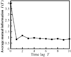
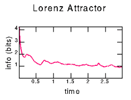
While it is easy to evaluate the linear autocorrelation between measurements as a function of $\mathrm{T}$, the usual criterion of seeking a zero in that quantity only leads to a value of $\mathrm{T}$ where the measurements are linearly independent. The dynamical interest of this is rather small. A much more motivated criterion, though harder to evaluate, was suggested by Fraser and Swinney in 1986: evaluate the average mutual information between measurements at time $n$ and time $n-T$;look for the first minimum in this quantity. This tells us when the two measurements are nenlinearly relatively independent, and this may provide a useful choice for $\mathrm{T}$ [17-21].
Decomposition models in time series are used to identify and describe trend and seasonal factors. Decomposition means to break down into simpler parts. When decomposition models are used, we can identify these patterns/factors separately. Some seasonal patterns of a time series model can be describe as festive season effects, holiday effects. As an example think that there is a festive season effect on sales of a textiles company, the company cannot clearly identify how its sales behave in long term. Therefore we can use this method to remove seasonal effects of the time series data set and then try to identify what kind of a trend, these sales have in long term (do the sales increase or decrease annually?) There are two types of decomposition models. They are additive models and multiplicative models.
Additive model is expressed as: $\mathrm{Y}=\mathrm{T}+\mathrm{S}+\mathrm{C}+\mathrm{I}$.
Multiplicative model is expressed as $\mathrm{Y}=\mathrm{T}^* \mathrm{~S} * \mathrm{C} * \mathrm{I}$. ( $\mathrm{Y}=$ Time Series Data , T=Trend, $\mathrm{S}=$ seasonal , $\mathrm{C}=$ Cynical , $\mathrm{I}=$ Irregular) Some decomposition models are expressed without cynical patterns. They can be written as below
Multiplicative: $\mathrm{Y}=$ Trend $^*$ Seasonal * Irregular When seasonal variation is relatively constant over time additive model is useful. When seasonal variation is increasing over time multiplicative model is useful. Multiplicative models are useful in economic and business data modeling. The aim of analyzing a time series is to understand and identify the patterns in a time series variable, therefore a variable with more observation outputs better results. As an example in each year Textiles Pvt Ltd sell cloths worth of $\$ 30000$ in December, where in other months they earn between $\$ 15000$ to $\$ 20000$. Then it is a constant seasonal variation. We can use additive model for this data series. But if the Textiles Pvt Ltd earns $\$ 30000$ in December 2018, $\$ 40000$ in December $2019, \$ 45000$ in December 2020, and earns between $\$ 15000$ to $\$ 20000$ every other month, then there is a visible increment of seasonal variation. We can use a multiplicative model for this data series. When multiplicative model $\mathrm{Y}=\mathrm{T}^* \mathrm{~S} * \mathrm{C}^* \mathrm{I}$ is transformed into log, then it becomes $\log \mathrm{Y}=\log \mathrm{T}+\log \mathrm{S}+\log \mathrm{C}+\log \mathrm{I}$.
Graphic method, semi-average method, curve fitting by principles and moving average method are used to measure trend.
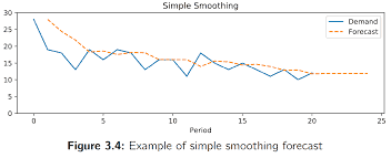
Single exponential smoothing is suitable for the models which don’t show a clear trend or a seasonal pattern. Exponential smoothing is used for forecasting economics and financial data. If there is a time series without a clear pattern then we can use exponential smoothing. But if there is a clear pattern then we should use moving averages.
We can use this method to forecast univariate time series. It can be used as an alternative to ARIMA models. While calculating this model past observations get weighted and they are weighted with a geometrically decreasing ratio. Exponential smooth forecasting is a weighted average forecast of past observations.
In single exponential smoothing, smoothing coefficient is called alpha $\alpha$. Alpha is always between 0 to 1 . Smaller alpha values indicate that there is more impact from past observations. Values close to 1 indicates that only most recent past observations has an influence on the predictions. Alpha is the smoothing constant. Alpha is normally selected between $0.1$ and $0.3$ in practical calculations.
Note: univariate data series is a data series with a single variable. The observations of these data series are recorded according to the time. Example: Annual inflation rate of USA.
Double exponential smoothing is more applicable for univariate data series with trend. Double exponential smoothing has alpha $\alpha$ and also an additional smoothing factor called $\beta$. Double exponential smoothing with additive trend is referred as Holt’s linear trend model. Double exponential smoothing with an exponential trend is used for the data series with multiplicative trend. These smoothing techniques are used to remove the trend and make the line straight. This method of making the line straight is called damping in time series. This idea was introduced by Gardner \& McKenzie in 1985.
统计代写|时间序列分析代写Time-Series Analysis代考|Moving Average
Moving average method removes short term patterns from a time series. It is a time series smoothing method. Moving average method is better for removing short term patterns.
Moving average is calculated by taking the average for set of observations inside a time series. For a time series with odd numbers of observations Moving average can be calculated by taking the average of 3,5,7 nearby observations. When the numbers of observations are even, then use moving average for time intervals of 2 or 4 . When less observations are taken to count the average, then the line become smoother. That means when a moving average is calculate for time periods of 3 , that line is smoother than a line which is calculated for time periods of 5 . These time intervals are called length of moving average. The length can be 2,3,4,5 or more. But the fitted line is smoother when the length is smaller.
Moving Average method is better than free hand method and semi average method. But when there are outliers or unusual values, this method is not efficient. If there are outliers then it will results unusual curves in the estimated line. Another disadvantage of this method is lacking observations at the first and last places in the newly created array. Now let’s do a sample on simple moving average.
统计代写|时间序列分析代写Time-Series Analysis代考|What is a stationary time series
Stationary Time Series Stationary time series models are time series that the mean and the variance of the variable don’t depend on the time. Therefore the mean and variance of a stationary time series are constant. They do not have any periodic fluctuations. A stationary time series is simply a stochastic process with constant mean and variance. There are strong stationary series and weak stationary series. When the distribution of the time series is same as the lagged time series, then it has a strong form of stationary. When the mean and correlation function of a time series does not change by shift in time it is a weak stationary time series. Auto covariance function is not a function of time. Stationary series is spread around the mean line in a given range. Below is a graph of a stationary time series. Stationary series spread around the mean line in a given range or given upper and lower limits. It has neither trend nor seasonality.
Non Stationary Time Series Trend, seasonal, cyclic and random patterned series fall under non stationary series. In order to do predictions on a non stationary series, it should be transformed into a stationary series.
Stochastic Process Stochastic process is a collection of random variables. Time series with the time variable is a basic type of a stochastic process. It is a model for the analysis. This can also be called as random process Mean of a stochastic process $\mu_t=\mathrm{E}\left(y_t\right)$ Where $\mathrm{t}=0, \pm 1, \pm 2 \ldots, \pm \mathrm{n}$ Autocovariance of stochastic process $y_{t, s}=\operatorname{Cov}\left(y_t, y_s\right)$ $\operatorname{Cov}\left(y_t, y_s\right)=\mathrm{E}\left(y_t-\mu_t\right)\left(y_s-\mu_s\right)$ Where $t, s=0, \pm 1, \pm 2 \ldots, \pm n$