月度归档： 2023 年 6 月

经济代写|宏观经济学代写Macroeconomics代考|Consumer Surplus

Posted on 2023年6月30日2023年6月30日 by statistics-lab

如果你也在怎样代写宏观经济学Macroeconomics 这个学科遇到相关的难题，请随时右上角联系我们的24/7代写客服。宏观经济学Macroeconomics对国家或地区经济整体行为的研究。它关注的是对整个经济事件的理解，如商品和服务的生产总量、失业水平和价格的一般行为。宏观经济学关注的是经济体的表现–经济产出、通货膨胀、利率和外汇兑换率以及国际收支的变化。减贫、社会公平和可持续增长只有在健全的货币和财政政策下才能实现。

宏观经济学Macroeconomics（来自希腊语前缀makro-，意思是 “大 “+经济学）是经济学的一个分支，处理整个经济体的表现、结构、行为和决策。例如，使用利率、税收和政府支出来调节经济的增长和稳定。这包括区域、国家和全球经济。根据经济学家Emi Nakamura和Jón Steinsson在2018年的评估，经济 “关于不同宏观经济政策的后果的证据仍然非常不完善，并受到严重批评。宏观经济学家研究的主题包括GDP（国内生产总值）、失业（包括失业率）、国民收入、价格指数、产出、消费、通货膨胀、储蓄、投资、能源、国际贸易和国际金融。

statistics-lab™ 为您的留学生涯保驾护航在代写宏观经济学Macroeconomics方面已经树立了自己的口碑, 保证靠谱, 高质且原创的统计Statistics代写服务。我们的专家在代写宏观经济学Macroeconomics代写方面经验极为丰富，各种代写宏观经济学Macroeconomics相关的作业也就用不着说。

经济代写|宏观经济学代写Macroeconomics代考|Consumer Surplus

In a competitive market, consumers and producers buy and sell at the market equilibrium price. However, some consumers will be willing and able to pay more for the good than they have to. But they would never knowingly buy something that is worth less to them. That is, what a consumer actually pays for a unit of a good is usually less than the amount she is willing to pay. For example, would you be willing to pay more than the market price for a rope ladder to get out of a burning building? Would you be willing to pay more than the market price for a tank of gasoline if you had run out of gas on a desolate highway in the desert? Would you be willing to pay more than the market price for an anti-venom shot if you had been bitten by a rattlesnake? Consumer surplus is the monetary difference between the amount a consumer is willing and able to pay for an additional unit of a good and what the consumer actually paysthe market price. Consumer surplus for the whole market is the sum of all the individual consumer surpluses for those consumers who have purchased the good.

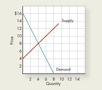
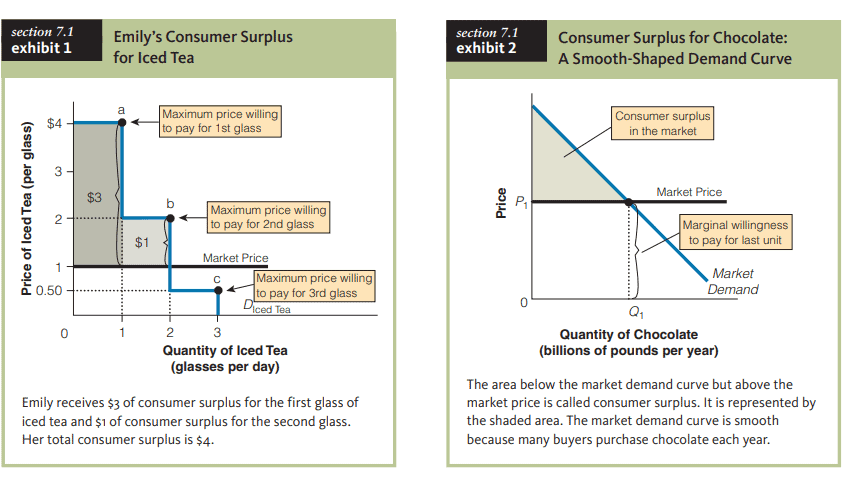
Suppose it is a hot day and iced tea is going for $\$ 1$ per glass, but Emily is willing to pay $\$ 4$ for the first glass (point a), $\$ 2$ for the second glass (point b), and $\$ 0.50$ for the third glass (point c), reflecting the law of demand. How much consumer surplus will Emily receive? First, it is important to note the general fact that if the consumer is a buyer of several units of a good, the earlier units will have greater marginal value and therefore create more consumer surplus because marginal willingness to pay falls as greater quantities are consumed in any period. In fact, you can think of the demand curve as a marginal benefit curve-the additional benefit derived from consuming one more unit. Notice in Exhibit 1 that Emily’s demand curve for iced tea has a step-like shape. This is demonstrated by Emily’s willingness to pay $\$ 4$ and $\$ 2$ successively for the first two glasses of iced tea. Thus, Emily will receive $\$ 3$ of consumer surplus for the first glass $(\$ 4-\$ 1)$ and $\$ 1$ of consumer surplus for the second glass $(\$ 2-\$ 1)$, for a total consumer surplus of $\$ 4$, as seen in Exhibit 1 . Emily will not be willing to purchase the third glass because her willingness to pay is less than its price $(\$ 0.50$ versus $\$ 1.00)$.
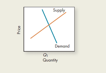
In Exhibit 2, we can easily measure the consumer surplus in the market by using a market demand curve rather than an individual demand curve. In short, the market consumer surplus is the area under the market demand curve and above the market price (the shaded area in Exhibit 2). The market for chocolate contains millions of potential buyers, so we will get a smooth demand curve. That is, each of the millions of potential buyers has their own willingness to pay. Because the demand curve represents the marginal benefits consumers receive from consuming an additional unit, we can conclude that all buyers of chocolate receive at least some consumer surplus in the market because the marginal benefit is greater than the market price-the shaded area in Exhibit 2 .

经济代写|宏观经济学代写Macroeconomics代考|Price Changes and Changes in Consumer Surplus

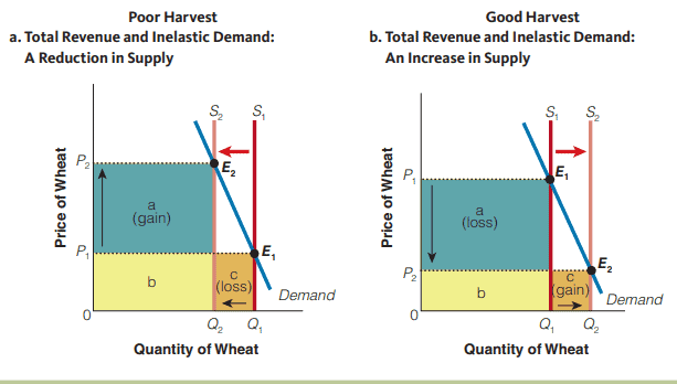
We may want to know how much consumers are hurt or helped when prices change. So let’s see what happens to consumer surplus when the price of a good rises or falls, when demand remains constant. Suppose that the price of your favorite beverage fell because of an increase in supply. Wouldn’t you feel better off? An increase in supply and a lower price will increase your consumer surplus for each unit you were already consuming and will also increase your consumer surplus from additional purchases at the lower price. Conversely, a decrease in supply and increase in price will lower your consumer surplus.

Exhibit 3 shows the gain in consumer surplus associated with a fall in the market price of pizza from $P_1$ to $P_2$. The fall in the market price leads to an increase in quantity demanded and an increase in consumer surplus. More specifically, consumer surplus increases from area $P_1 \mathrm{AB}$ to area $P_2 \mathrm{AC}$, for a gain in consumer surplus of $P_1 B C P_2$. The increase in consumer surplus has two parts. First, there is an increase in consumer surplus, because $Q_1$ can now be purchased at a lower price; this amount of additional consumer surplus is illustrated by area $P_1 \mathrm{BDP}_2$ in Exhibit 3. That is, these consumers would have purchased those pizzas at the original price of $P_1$, but now can purchase them at the new lower price of $P_2$. Second, the lower price makes it advantageous for buyers to expand their purchases from $Q_1$ to $Q_2$. The net benefit to buyers from expanding their consumption from $Q_1$ to $Q_2$ is illustrated by area BCD. That is, buyers would purchase those additional pizzas because the price was reduced. Similarly, if the market price of pizzas rose, the quantity demanded would fall. As a result, the two effects triggered by a decrease in price would increase consumer surplus, while an increase in price would decrease consumer surplus by $P_1 \mathrm{BCP}_2$.

In sum, consumer surplus measures the net gains buyers perceive that they receive, over and above the market price they must pay. So in this sense, it is a good measure of changes in economic well-being, if we assume that individuals make rational choices-self-betterment choices-and that individuals are the best judges of how much benefit they derive from goods and services.

宏观经济学代考

经济代写|宏观经济学代写Macroeconomics代考|Consumer Surplus

在竞争市场中，消费者和生产者以市场均衡价格进行买卖。然而，一些消费者愿意并且有能力为这些商品支付比他们必须支付的更多的钱。但他们永远不会故意购买对他们来说价值较低的东西。也就是说，消费者为一单位商品实际支付的价格通常低于她愿意支付的价格。例如，你愿意花比市场价更高的价格买一个绳梯从着火的大楼里出来吗?如果你在荒凉的沙漠公路上没油了，你愿意花比市场价更高的价钱买一箱汽油吗?如果你被响尾蛇咬了，你会愿意花比市场价更高的价钱去打一针抗蛇毒疫苗吗?消费者剩余是消费者愿意和能够为一单位额外商品支付的金额与消费者实际支付的市场价格之间的货币差额。整个市场的消费者剩余是购买了该商品的消费者的所有个人消费者剩余的总和。

假设天气很热，冰茶的价格是每杯1美元，但艾米丽愿意花4美元买第一杯(a点)，花2美元买第二杯(b点)，花0.50美元买第三杯(c点)，这反映了需求定律。艾米丽会得到多少消费者剩余?首先，重要的是要注意这样一个普遍的事实，即如果消费者是一种商品的几个单位的购买者，那么较早的单位将具有更大的边际价值，从而产生更多的消费者剩余，因为边际支付意愿随着任何时期消费数量的增加而下降。事实上，你可以把需求曲线看作边际效益曲线——多消费一单位产品所产生的额外效益。注意，在图表1中，艾米丽对冰茶的需求曲线呈阶梯状。艾米丽愿意为前两杯冰茶连续支付$ $ 4和$ $ 2就证明了这一点。因此，艾米丽将从第一杯酒中获得$ $ $ 3的消费者剩余$ $($ $ 4- $ $ 1)$，从第二杯酒中获得$ $ $ 1的消费者剩余$ $ $($ $ 2- $ $ 1)$，总的消费者剩余$ $ $ 4，如表1所示。艾米丽不愿意购买第三个杯子，因为她的支付意愿低于它的价格(0.50美元对1.00美元)。
在表2中，我们可以很容易地通过使用市场需求曲线而不是个人需求曲线来衡量市场中的消费者剩余。简而言之，市场消费者剩余是市场需求曲线下方和市场价格上方的面积(图2中的阴影区域)。巧克力市场包含数百万潜在买家，因此我们将得到一条平滑的需求曲线。也就是说，数百万潜在买家中的每个人都有自己的支付意愿。因为需求曲线代表消费者从额外消费一单位中获得的边际效益，我们可以得出结论，所有巧克力的购买者在市场上至少获得了一些消费者剩余，因为边际效益大于市场价格(图2中的阴影区域)。

经济代写|宏观经济学代写Macroeconomics代考|Price Changes and Changes in Consumer Surplus

我们可能想知道价格变化对消费者的伤害或帮助有多大。看看需求保持不变时，商品价格上升或下降时，消费者剩余会怎样。假设你最喜欢的饮料的价格因为供给的增加而下降。你会不会感觉好些?供给的增加和较低的价格会增加你已经消费的每单位的消费者剩余，也会增加你在较低价格下额外购买的消费者剩余。相反，供给的减少和价格的增加会降低消费者剩余。

图3显示了消费者剩余的增加与披萨市场价格从$P_1$下降到$P_2$有关。市场价格的下跌导致需求量的增加和消费者剩余的增加。更具体地说，消费者剩余从面积$P_1 \ mathm {AB}$增加到面积$P_2 \ mathm {AC}$，消费者剩余增加$P_1 B C P_2$。消费者剩余的增加有两个部分。首先，消费者剩余增加，因为Q_1美元现在可以以更低的价格购买;这个数量的额外消费者剩余在表3中用面积$P_1 \ mathm {BDP}_2$表示。也就是说，这些消费者会以原价$P_1$购买这些披萨，但现在可以以新的较低价格$P_2$购买。其次，较低的价格有利于买家将购买金额从$Q_1$扩大到$Q_2$。购买者将消费从$Q_1$扩大到$Q_2$的净收益用面积BCD表示。也就是说，买家会因为价格降低而购买那些额外的披萨。同样，如果披萨的市场价格上涨，需求量就会下降。结果表明，价格下降引起的两种效应均使消费者剩余增加，而价格上涨则使消费者剩余减少$P_1 \ mathm {BCP}_2$。

总而言之，消费者剩余衡量的是购买者认为他们获得的净收益，高于他们必须支付的市场价格。因此，从这个意义上说，如果我们假设个人做出理性选择——自我改善的选择——并且个人是他们从商品和服务中获得多少利益的最佳判断者，那么它是衡量经济福祉变化的一个很好的指标。

经济代写|宏观经济学代写Macroeconomics代考请认准statistics-lab™

统计代写请认准statistics-lab™. statistics-lab™为您的留学生涯保驾护航。

金融工程代写

金融工程是使用数学技术来解决金融问题。金融工程使用计算机科学、统计学、经济学和应用数学领域的工具和知识来解决当前的金融问题，以及设计新的和创新的金融产品。

非参数统计代写

非参数统计指的是一种统计方法，其中不假设数据来自于由少数参数决定的规定模型；这种模型的例子包括正态分布模型和线性回归模型。

广义线性模型代考

广义线性模型（GLM）归属统计学领域，是一种应用灵活的线性回归模型。该模型允许因变量的偏差分布有除了正态分布之外的其它分布。

术语广义线性模型（GLM）通常是指给定连续和/或分类预测因素的连续响应变量的常规线性回归模型。它包括多元线性回归，以及方差分析和方差分析（仅含固定效应）。

有限元方法代写

有限元方法（FEM）是一种流行的方法，用于数值解决工程和数学建模中出现的微分方程。典型的问题领域包括结构分析、传热、流体流动、质量运输和电磁势等传统领域。

有限元是一种通用的数值方法，用于解决两个或三个空间变量的偏微分方程（即一些边界值问题）。为了解决一个问题，有限元将一个大系统细分为更小、更简单的部分，称为有限元。这是通过在空间维度上的特定空间离散化来实现的，它是通过构建对象的网格来实现的：用于求解的数值域，它有有限数量的点。边界值问题的有限元方法表述最终导致一个代数方程组。该方法在域上对未知函数进行逼近。[1] 然后将模拟这些有限元的简单方程组合成一个更大的方程系统，以模拟整个问题。然后，有限元通过变化微积分使相关的误差函数最小化来逼近一个解决方案。

tatistics-lab作为专业的留学生服务机构，多年来已为美国、英国、加拿大、澳洲等留学热门地的学生提供专业的学术服务，包括但不限于Essay代写，Assignment代写，Dissertation代写，Report代写，小组作业代写，Proposal代写，Paper代写，Presentation代写，计算机作业代写，论文修改和润色，网课代做，exam代考等等。写作范围涵盖高中，本科，研究生等海外留学全阶段，辐射金融，经济学，会计学，审计学，管理学等全球99%专业科目。写作团队既有专业英语母语作者，也有海外名校硕博留学生，每位写作老师都拥有过硬的语言能力，专业的学科背景和学术写作经验。我们承诺100%原创，100%专业，100%准时，100%满意。

随机分析代写

随机微积分是数学的一个分支，对随机过程进行操作。它允许为随机过程的积分定义一个关于随机过程的一致的积分理论。这个领域是由日本数学家伊藤清在第二次世界大战期间创建并开始的。

时间序列分析代写

随机过程，是依赖于参数的一组随机变量的全体，参数通常是时间。随机变量是随机现象的数量表现，其时间序列是一组按照时间发生先后顺序进行排列的数据点序列。通常一组时间序列的时间间隔为一恒定值（如1秒，5分钟，12小时，7天，1年），因此时间序列可以作为离散时间数据进行分析处理。研究时间序列数据的意义在于现实中，往往需要研究某个事物其随时间发展变化的规律。这就需要通过研究该事物过去发展的历史记录，以得到其自身发展的规律。

回归分析代写

多元回归分析渐进（Multiple Regression Analysis Asymptotics）属于计量经济学领域，主要是一种数学上的统计分析方法，可以分析复杂情况下各影响因素的数学关系，在自然科学、社会和经济学等多个领域内应用广泛。

MATLAB代写

MATLAB 是一种用于技术计算的高性能语言。它将计算、可视化和编程集成在一个易于使用的环境中，其中问题和解决方案以熟悉的数学符号表示。典型用途包括：数学和计算算法开发建模、仿真和原型制作数据分析、探索和可视化科学和工程图形应用程序开发，包括图形用户界面构建MATLAB 是一个交互式系统，其基本数据元素是一个不需要维度的数组。这使您可以解决许多技术计算问题，尤其是那些具有矩阵和向量公式的问题，而只需用 C 或 Fortran 等标量非交互式语言编写程序所需的时间的一小部分。MATLAB 名称代表矩阵实验室。MATLAB 最初的编写目的是提供对由 LINPACK 和 EISPACK 项目开发的矩阵软件的轻松访问，这两个项目共同代表了矩阵计算软件的最新技术。MATLAB 经过多年的发展，得到了许多用户的投入。在大学环境中，它是数学、工程和科学入门和高级课程的标准教学工具。在工业领域，MATLAB 是高效研究、开发和分析的首选工具。MATLAB 具有一系列称为工具箱的特定于应用程序的解决方案。对于大多数 MATLAB 用户来说非常重要，工具箱允许您学习和应用专业技术。工具箱是 MATLAB 函数（M 文件）的综合集合，可扩展 MATLAB 环境以解决特定类别的问题。可用工具箱的领域包括信号处理、控制系统、神经网络、模糊逻辑、小波、仿真等。

R语言代写	问卷设计与分析代写
PYTHON代写	回归分析与线性模型代写
MATLAB代写	方差分析与试验设计代写
STATA代写	机器学习/统计学习代写
SPSS代写	计量经济学代写
EVIEWS代写	时间序列分析代写
EXCEL代写	深度学习代写
SQL代写	各种数据建模与可视化代写

经济代写|宏观经济学代写Macroeconomics代考|How Does the Price Elasticity of Demand Impact Total Revenue?

Posted on 2023年6月30日2023年6月30日 by statistics-lab

经济代写|宏观经济学代写Macroeconomics代考|Proportion of Income Spent on the Good

The price elasticity of demand for a good also has implications for total revenue. Total revenue (TR) is the amount sellers receive for a good or service. Total revenue is simply the price of the good $(P)$ times the quantity of the good sold $(Q): T R=P \times Q$. The elasticity of demand will help to predict how changes in the price will impact total revenue earned by the producer for selling the good. Let’s see how this works.

In Exhibit 1 , we see that when the demand is price elastic $\left(E_{\mathrm{D}}>1\right)$, total revenues will rise as the price declines, because the percentage increase in the quantity demanded is greater than the percentage reduction in price. For example, if the price of a good is cut in half (say from $\$ 10$ to $\$ 5$ ) and the quantity demanded more than doubles (say from 40 to 100 ), total revenue will rise from $\$ 400(\$ 10 \times 40=\$ 400)$ to $\$ 500(\$ 5 \times 100=\$ 500)$. Equivalently, if the price rises from $\$ 5$ to $\$ 10$ and the quantity demanded falls from 100 to 40 units, then total revenue will fall from $\$ 500$ to $\$ 400$. As this example illustrates, if the demand curve is relatively elastic, total revenue will vary inversely with a price change.

You can see from the following what happens to total revenue when demand is price elastic. (Note: The size of the price and quantity arrows represents the size of the percentage changes.)
When Demand Is Price Elastic
$$
\downarrow T R=\uparrow P \times \downarrow Q
$$
or
$$
\uparrow T R=\downarrow P \times \uparrow Q
$$
On the other hand, if demand for a good is relatively inelastic $\left(E_{\mathrm{D}}<1\right)$, the total revenue will be lower at lower prices than at higher prices because a given price reduction will be accompanied by a proportionately smaller increase in quantity demanded. For example, as shown in Exhibit 2, if the price of a good is cut (say from $\$ 10$ to $\$ 5$ ) and the quantity demanded less than doubles (say it increases from 30 to 40 ), then total revenue will fall from $\$ 300(\$ 10 \times 30=\$ 300)$ to $\$ 200(\$ 5 \times 40=\$ 200)$. Equivalently, if the price increases from $\$ 5$ to $\$ 10$ and the quantity demanded falls from 40 to 30 , total revenue will increase from $\$ 200$ to $\$ 300$. That is, if the demand curve is inelastic, total revenue will vary directly with a price change.
When Demand Is Price Inelastic
$$
\begin{aligned}
\uparrow T R= & \uparrow P \times \downarrow Q \
& \text { or } \
\downarrow T R= & \downarrow P \times \uparrow Q
\end{aligned}
$$
or
In this case, the “net” effect on total revenue is reversed but easy to see. (Again, the size of the price and quantity arrows represents the size of the percentage changes.)

经济代写|宏观经济学代写Macroeconomics代考|Price Elasticity Changes along a Linear Demand Curve

As already shown (Section 6.1, Exhibit 1), the slopes of demand curves can be used to estimate their relative elasticities of demand: The steeper one demand curve is relative to another, the more inelastic it is relative to the other. However, except for the extreme cases of perfectly elastic and perfectly inelastic curves, great care must be taken when trying to estimate the degree of elasticity of one demand curve from its slope. In fact, as we will soon see, a straight-line demand curve with a constant slope will change elasticity continuously as you move up or down it. It is because the slope is the ratio of changes in the two variables (price and quantity) while the elasticity is the ratio of percentage changes in the two variables.

We can easily demonstrate that the elasticity of demand varies along a linear demand curve by using what we already know about the interrelationship between price and total revenue.

Exhibit 4 shows a linear (constant slope) demand curve. In Exhibit 4(a), we see that when the price falls on the upper half of the demand curve from $P_1$ to $P_2$, and quantity demanded increases from $Q_1$ to $Q_2$, total revenue increases. That is, the new area of total revenue $($ area $b+c$ ) is larger than the old area of total revenue (area $a+b)$. It is also true that if price increased in this region (from $P_2$ to $P_1$ ), total revenue would fall because $\mathrm{b}+\mathrm{c}$ is greater than $\mathrm{a}+\mathrm{b}$.

In this region of the demand curve, then, there is a negative relationship between price and total revenue. As we discussed earlier, this is characteristic of an elastic demand curve $\left(E_{\mathrm{D}}>1\right)$.
Exhibit 4(b) illustrates what happens to total revenue on the lower half of the same demand curve. When the price falls from $P_3$ to $P_4$ and the quantity demanded increases from $Q_3$ to $Q_4$, total revenue actually decreases because the new area of total revenue (area $\mathrm{e}+\mathrm{f}$ ) is less than the old area of total revenue (area $\mathrm{d}+\mathrm{e}$ ). Likewise, it is clear that an increase in price from $P_4$ to $P_3$ would increase total revenue. In this case, there is a positive relationship between price and total revenue, which, as we discussed, is characteristic of an inelastic demand curve $\left(E_{\mathrm{D}}<1\right)$. Together, parts (a) and (b) of Exhibit 4 illustrate that, although the slope remains constant, the elasticity of a linear demand curve changes along the length of the curve-from relatively elastic at higher price ranges to relatively inelastic at lower price ranges.

宏观经济学代考

经济代写|宏观经济学代写Macroeconomics代考|Proportion of Income Spent on the Good

商品需求的价格弹性也会影响总收入。总收益(TR)是卖方从商品或服务中获得的金额。总收入就是商品的价格$(P)$乘以商品的销售量$(Q): T R=P \times Q$。需求弹性将有助于预测价格的变化将如何影响生产者销售商品所获得的总收入。让我们看看它是如何工作的。

在表1中，我们看到，当需求具有价格弹性$\left(E_{\mathrm{D}}>1\right)$时，总收益将随着价格下降而上升，因为需求量增加的百分比大于价格下降的百分比。例如，如果一种商品的价格减半(比如从$\$ 10$降至$\$ 5$)，而需求量增加一倍以上(比如从40降至100)，总收入将从$\$ 400(\$ 10 \times 40=\$ 400)$上升至$\$ 500(\$ 5 \times 100=\$ 500)$。同样地，如果价格从$\$ 5$上升到$\$ 10$，需求量从100下降到40，那么总收益将从$\$ 500$下降到$\$ 400$。如本例所示，如果需求曲线是相对弹性的，总收入将与价格变化成反比。

从下图可以看出，当需求具有价格弹性时，总收入的变化情况。(注:价格和数量箭头的大小代表百分比变化的大小。)
当需求具有价格弹性时
$$
\downarrow T R=\uparrow P \times \downarrow Q
$$
或
$$
\uparrow T R=\downarrow P \times \uparrow Q
$$
另一方面，如果对一种商品的需求相对缺乏弹性$\left(E_{\mathrm{D}}<1\right)$，则总收益在价格较低时将低于价格较高时，因为给定的价格降低将伴随着按比例较小的需求量增加。例如，如图2所示，如果一种商品的价格降低(比如从$\$ 10$降至$\$ 5$)，而需求量增加一倍以下(比如从30增加到40)，那么总收入将从$\$ 300(\$ 10 \times 30=\$ 300)$降至$\$ 200(\$ 5 \times 40=\$ 200)$。同样，如果价格从$\$ 5$上升到$\$ 10$，需求量从40下降到30，总收益将从$\$ 200$上升到$\$ 300$。也就是说，如果需求曲线是非弹性的，总收入将直接随价格变化而变化。
当需求价格无弹性时
$$
\begin{aligned}
\uparrow T R= & \uparrow P \times \downarrow Q \
& \text { or } \
\downarrow T R= & \downarrow P \times \uparrow Q
\end{aligned}
$$
或
在这种情况下，对总收入的“净”影响是相反的，但很容易看到。(同样，价格和数量箭头的大小表示百分比变化的大小。)

经济代写|宏观经济学代写Macroeconomics代考|Price Elasticity Changes along a Linear Demand Curve

如前所述(第6.1节，表1)，需求曲线的斜率可以用来估计需求的相对弹性:一条需求曲线相对于另一条需求曲线越陡峭，它相对于另一条需求曲线的弹性就越小。然而，除了完全弹性曲线和完全非弹性曲线的极端情况外，在试图从一条需求曲线的斜率估计其弹性程度时，必须非常小心。事实上，我们很快就会看到，斜率为常数的直线需求曲线会随着上下移动而不断改变弹性。这是因为斜率是两个变量(价格和数量)变化的比率，而弹性是两个变量变化百分比的比率。

通过使用我们已经知道的价格和总收入之间的相互关系，我们可以很容易地证明需求弹性沿着线性需求曲线变化。

图4显示了一条线性(斜率恒定)需求曲线。在图4(a)中，我们看到，当价格在需求曲线的上半部分从$P_1$下降到$P_2$时，需求量从$Q_1$增加到$Q_2$，总收入增加。也就是说，总收入的新区域$(区域$b+c$)大于总收入的旧区域$(区域$a+b)$。同样，如果该区域的价格上涨(从$P_2$到$P_1$)，总收益将下降，因为$\ mathm {b}+\ mathm {c}$大于$\ mathm {a}+\ mathm {b}$。

因此，在需求曲线的这个区域，价格和总收入之间存在负相关关系。正如我们前面所讨论的，这是弹性需求曲线$\left(E_{\ mathm {D}}>1\right)$的特征。
图4(b)展示了同一需求曲线下半部分的总收入。当价格从$P_3$下降到$P_4$，需求量从$Q_3$增加到$Q_4$时，总收入实际上减少了，因为总收入的新区域($\ mathm {e}+\ mathm {f}$)小于总收入的旧区域($\ mathm {d}+\ mathm {e}$)。同样，很明显，价格从$P_4$增加到$P_3$会增加总收入。在这种情况下，价格和总收入之间存在正关系，正如我们所讨论的，这是非弹性需求曲线$\left(E_{\ mathm {D}}<1\right)$的特征。图4的(a)和(b)部分共同说明，尽管斜率保持不变，但线性需求曲线的弹性沿着曲线的长度变化——从较高价格区间的相对弹性到较低价格区间的相对无弹性。

统计代写请认准statistics-lab™. statistics-lab™为您的留学生涯保驾护航。

金融工程代写

非参数统计代写

非参数统计指的是一种统计方法，其中不假设数据来自于由少数参数决定的规定模型；这种模型的例子包括正态分布模型和线性回归模型。

广义线性模型代考

广义线性模型（GLM）归属统计学领域，是一种应用灵活的线性回归模型。该模型允许因变量的偏差分布有除了正态分布之外的其它分布。

有限元方法代写

随机分析代写

时间序列分析代写

回归分析代写

MATLAB代写

R语言代写	问卷设计与分析代写
PYTHON代写	回归分析与线性模型代写
MATLAB代写	方差分析与试验设计代写
STATA代写	机器学习/统计学习代写
SPSS代写	计量经济学代写
EVIEWS代写	时间序列分析代写
EXCEL代写	深度学习代写
SQL代写	各种数据建模与可视化代写

经济代写|宏观经济学代写Macroeconomics代考|Price Controls

Posted on 2023年6月30日2023年6月30日 by statistics-lab

经济代写|宏观经济学代写Macroeconomics代考|Price Controls

Although non-equilibrium prices can occur naturally in the private sector, reflecting uncertainty, they seldom last for long. Governments, however, may impose non-equilibrium prices for significant periods. Price controls involve the use of the power of the state to establish prices different from the equilibrium prices that would otherwise prevail. The motivations for price controls vary with the market under consideration. For example, a price ceiling, a legal maximum price, is often set for goods deemed important to low-income households, such as housing. Or a price floor, a legal minimum price, may be set on wages because wages are the primary source of income for most people.

Price controls are not always implemented by the federal government. Local governments (and more rarely, private companies) can and do impose local price controls. One fairly wellknown example is rent control. The inflation of the late 1970 s meant rapidly rising rents; some communities, such as Santa Monica, California, decided to do something about it. In response, they limited how much landlords could charge for rental housing.

Price Ceilings: Rent Controls
Rent control experiences can be found in many cities across the country. San Francisco, Berkeley, and New York City all have had some form of rent control. Although the rules may vary from city to city and over time, generally the price (or rent) of an apartment remains fixed over the tenure of an occupant, except for allowable annual increases tied to the cost of living or some other price index. When an occupant moves out, the owners can usually, but not always, raise the rent to a near-market level for the next occupant. The controlled rents for existing occupants, however, are generally well below market rental rates.

Results of Rent Controls
Most people living in rent-controlled apartments are getting a good deal, one that they would lose by moving as their family circumstances or income changes. Tenants thus are reluctant to give up their governmentally granted right to a below-market-rent apartment. In addition, because the rents received by landlords are constrained and below market levels, the rate of return (roughly, the profit) on housing investments falls compared with that on other forms of real estate not subject to rent controls, such as office rents or mortgage payments on condominiums. Hence, the incentive to construct new housing is reduced.

Furthermore, when landlords are limited in the rents they can charge, they have little incentive to improve or upgrade apartments-by putting in new kitchen appliances or new carpeting, for instance. In fact, rent controls give landlords some incentive to avoid routine maintenance, thereby lowering the cost of apartment ownership to a figure approximating the controlled rental price, although the quality of the housing stock will deteriorate over time. Another impact of rent controls is that they promote housing discrimination. Where rent controls do not exist, prejudiced landlords might willingly rent to people they believe are undesirable simply because the undesirables are the only ones willing to pay the requested rents (and the landlords are not willing to lower their rents substantially to get desirable renters because of the possible loss of thousands of dollars in income). With rent controls, each rent-controlled apartment is likely to attract many possible renters, some desirable and some undesirable as judged by the landlord, simply because the rent is at a below-equilibrium price. Landlords can indulge in their “taste” for discrimination without any additional financial loss beyond that required by the controls. Consequently, they will be more likely to choose to rent to desirable people, perhaps a family without children or pets, rather than to undesirable ones, perhaps a family with lower income and so a greater risk of nonpayment.

Exhibit 1 shows the impact of rent controls. If the price ceiling $\left(P_{\mathrm{RC}}\right)$ is set below the equilibrium price $\left(P_{\mathrm{E}}\right)$, consumers are willing to buy $Q_{\mathrm{D}}$, but producers are only willing to supply $Q_s$. The rent control policy will therefore create a persistent shortage, the difference between $Q_D$ and $Q_s$.

经济代写|宏观经济学代写Macroeconomics代考|Price Floors: The Minimum Wage

The argument for a minimum wage is simple: Existing wages for workers in some types of labor markets do not allow for a very high standard of living, and a minimum wage allows those workers to live better than before. Ever since 1938, when the first minimum wage was established (at 25 cents per hour), the federal government has, by legislation, made it illegal to pay most workers an amount below the current legislated minimum wage. In 2014 , the federal minimum wage was set at $\$ 7.25$. A number of states also have minimum-wage laws. In cases where an employee is subject to both state and federal minimum-wage laws, the employee is entitled to the higher minimum wage.

Let’s examine graphically the impact of a minimum wage on low-skilled workers. In Exhibit 2, suppose the government sets the minimum wage, $W_{M I N}$, above the market equilibrium wage, $W_{\mathrm{E}}$. In Exhibit 2, we see that the price floor is binding. That is, there is a surplus of low-skilled workers at $W_{\text {MIN }}$ because the quantity of labor supplied is greater than the quantity of labor demanded. The reason for the surplus of low-skilled workers (unemployment) at $W_{\mathrm{MIN}}$ is that more people are willing to work than employers are willing and able to hire.
Notice that not everyone loses from a minimum wage. Workers who continue to hold jobs have higher incomesthose between 0 and $Q_D$ in Exhibit 2. However, many lowskilled workers suffer from a minimum wage-those between $Q_D$ and $Q_S$ in Exhibit 2-because they either lose their jobs or are unable to get them in the first place. Although studies disagree somewhat on the precise magnitudes, they largely agree that minimum-wage laws do create some unemployment and that the unemployment is concentrated among teenagers-the least-experienced and least-skilled members of the labor force. Many teenagers are willing to accept the lower wage in exchange for on-the-job training. In fact, some college students accept non-paying intern jobs for the experience. Minimum-wage laws do not apply to internships, and if they did, many of those jobs might not exist.

宏观经济学代考

经济代写|宏观经济学代写Macroeconomics代考|Price Controls

尽管非均衡价格可以在私营部门自然出现，反映出不确定性，但它们很少持续很长时间。然而，政府可能在相当长的时期内强制实行非均衡价格。价格控制包括使用国家权力来制定不同于均衡价格的价格。价格管制的动机因所考虑的市场而异。例如，对于住房等被认为对低收入家庭很重要的商品，通常会设定价格上限，即法定最高价格。由于工资是大多数人的主要收入来源，因此可以对工资设定最低价格。

价格管制并不总是由联邦政府实施。地方政府(以及更罕见的私营企业)能够而且确实实施了地方价格控制。一个相当著名的例子是房租管制。20世纪70年代末的通货膨胀意味着租金迅速上涨;一些社区，如加利福尼亚州的圣莫尼卡，决定对此采取行动。作为回应，他们限制了房东出租房屋的收费。

价格上限:租金管制
全国许多城市都有房租管制的经验。旧金山、伯克利和纽约都有某种形式的租金管制。虽然这些规定可能因城市和时间而异，但一般来说，公寓的价格(或租金)在居住者的任期内保持不变，除了与生活成本或其他价格指数挂钩的允许年度上涨。当住户搬走时，业主通常可以(但并非总是如此)将租金提高到接近市场水平，以供下一位住户入住。然而，现有住户的管制租金一般远低于市场租金。

租金管制的结果
大多数住在租金管制公寓的人都得到了一笔不错的交易，而随着家庭环境或收入的变化，他们可能会因为搬家而失去这笔交易。因此，租户不愿意放弃政府授予的低于市场租金的公寓的权利。此外，由于房东收到的租金受到限制，低于市场水平，与不受租金管制的其他形式的房地产(如办公室租金或公寓的抵押贷款)相比，住房投资的回报率(大致是利润)下降。因此，建造新住房的动力减少了。

此外，当房东收取的租金有限时，他们几乎没有动力改善或升级公寓——例如，安装新的厨房电器或新地毯。事实上，租金管制给房东提供了一些避免日常维护的动力，从而将公寓拥有成本降低到接近受管制的租金价格，尽管住房质量会随着时间的推移而恶化。房租管制的另一个影响是助长了住房歧视。在租金管制不存在的地方，有偏见的房东可能愿意把房子租给他们认为不受欢迎的人，仅仅是因为不受欢迎的人是唯一愿意支付所要求的租金的人(房东不愿意大幅降低租金来获得理想的租户，因为可能会损失数千美元的收入)。在租金管制下，每套租金管制公寓可能会吸引许多潜在的租客，根据房东的判断，有些是可取的，有些是不可取的，仅仅是因为租金低于均衡价格。房东们可以尽情享受歧视的“滋味”，而不会在管制要求之外造成任何额外的经济损失。因此，他们更有可能选择把房子租给理想的人，也许是没有孩子或宠物的家庭，而不是不理想的人，也许是收入较低的家庭，因此有更大的拖欠风险。

表1显示了租金管制的影响。如果价格上限$\左(P_{\ mathm {RC}}\右)$低于均衡价格$\左(P_{\ mathm {E}}\右)$，则消费者愿意购买$Q_{\ mathm {D}}$，但生产者只愿意提供$Q_s$。因此，租金管制政策将造成持续短缺，即$Q_D$和$Q_s$之间的差额。

经济代写|宏观经济学代写Macroeconomics代考|Price Floors: The Minimum Wage

支持最低工资的理由很简单:在某些类型的劳动力市场上，现有的工人工资无法实现非常高的生活水平，而最低工资使这些工人的生活比以前更好。自从1938年确立第一个最低工资标准(每小时25美分)以来，联邦政府就通过立法规定，支付大多数工人低于现行法定最低工资是非法的。2014年，联邦最低工资定为7.25美元。许多州也有最低工资法。在雇员同时受州和联邦最低工资法约束的情况下，雇员有权获得较高的最低工资。

让我们来图解一下最低工资对低技能工人的影响。在表2中，假设政府将最低工资$W_{M I N}$设定在市场均衡工资$W_{\ mathm {E}}$之上。在表2中，我们看到价格下限是有约束力的。也就是说，在$W_{\text {MIN}}$处存在低技能工人的剩余，因为提供的劳动力数量大于需求的劳动力数量。低技能工人(失业率)过剩的原因是，愿意工作的人比雇主愿意和能够雇佣的人多。
请注意，并不是每个人都因最低工资而蒙受损失。在图表2中，继续工作的工人的收入在0到$Q_D$之间。然而，许多低技能工人受到最低工资的影响——图表2中那些在$Q_D$和$Q_S$之间的工人——因为他们要么失去了工作，要么一开始就找不到工作。尽管研究在具体数值上存在分歧，但它们基本上都同意，最低工资法确实造成了一些失业，而且失业集中在青少年——劳动力中经验最少、技能最低的成员。许多青少年愿意接受较低的工资，以换取在职培训。事实上，一些大学生为了获得经验而接受无薪实习工作。最低工资法并不适用于实习，如果适用的话，许多实习岗位可能就不存在了。

统计代写请认准statistics-lab™. statistics-lab™为您的留学生涯保驾护航。

金融工程代写

非参数统计代写

非参数统计指的是一种统计方法，其中不假设数据来自于由少数参数决定的规定模型；这种模型的例子包括正态分布模型和线性回归模型。

广义线性模型代考

广义线性模型（GLM）归属统计学领域，是一种应用灵活的线性回归模型。该模型允许因变量的偏差分布有除了正态分布之外的其它分布。

有限元方法代写

随机分析代写

时间序列分析代写

回归分析代写

MATLAB代写

R语言代写	问卷设计与分析代写
PYTHON代写	回归分析与线性模型代写
MATLAB代写	方差分析与试验设计代写
STATA代写	机器学习/统计学习代写
SPSS代写	计量经济学代写
EVIEWS代写	时间序列分析代写
EXCEL代写	深度学习代写
SQL代写	各种数据建模与可视化代写

经济代写|微观经济学代写Microeconomics代考|Determination of Exchange Rates and Trade

Posted on 2023年6月30日2023年6月30日 by statistics-lab

如果你也在怎样代写微观经济学Microeconomics 这个学科遇到相关的难题，请随时右上角联系我们的24/7代写客服。微观经济学Microeconomics是主流经济学的一个分支，研究个人和公司在做出有关稀缺资源分配的决策时的行为以及这些个人和公司之间的互动。微观经济学侧重于研究单个市场、部门或行业，而不是宏观经济学所研究的整个国民经济。

微观经济学Microeconomic的一个目标是分析在商品和服务之间建立相对价格的市场机制，并在各种用途之间分配有限资源。微观经济学显示了自由市场导致理想分配的条件。它还分析了市场失灵，即市场未能产生有效的结果。微观经济学关注公司和个人，而宏观经济学则关注经济活动的总和，处理增长、通货膨胀和失业问题以及与这些问题有关的国家政策。微观经济学还处理经济政策（如改变税收水平）对微观经济行为的影响，从而对经济的上述方面产生影响。

statistics-lab™ 为您的留学生涯保驾护航在代写微观经济学Microeconomics方面已经树立了自己的口碑, 保证靠谱, 高质且原创的统计Statistics代写服务。我们的专家在代写微观经济学Microeconomics代写方面经验极为丰富，各种代写微观经济学Microeconomics相关的作业也就用不着说。

经济代写|微观经济学代写Microeconomics代考|Determination of Exchange Rates and Trade

As mentioned above, transferable sources of comparative advantage aren’t the only way to eliminate trade imbalances. Exchange rates are another. The market for foreign currencies is called the foreign exchange (forex) market. It is this market that determines the exchange rates-the rate at which one country’s currency can be traded for another country’s currency – that newspapers report daily in tables such as the table below, which shows the cost of various currencies in terms of dollars and the cost of dollars in terms of those currencies.

The second column in this table reports the price of foreign currencies in terms of dollars. For example, one Argentinean peso costs about 22 cents. The third column tells you the price of dollars in terms of the foreign currency. For example, one U.S. dollar costs 4.5 Argentinean pesos.

People exchange currencies to buy goods or assets in other countries. For example, an American who wants to buy stock of a company that trades on the EU stock exchange first needs to buy euros with dollars. If the stock costs 150 euros, he will need to buy 150 euros. With an exchange rate of $\$ 1.30$ for 1 euro, he will need to pay $\$ 195$ to buy 150 euros $(\$ 1.30 \times 150)$. Only then can he buy the stock.

Let’s now turn to a graphical analysis of the forex market. At first glance, the graphical analysis of foreign exchange rates seems simple: You have an upward-sloping supply curve and a downward-sloping demand curve. But what goes on the axes? Obviously price and quantity, but what price? And what quantity? Because you are talking about the prices of currencies relative to each other, you have to specify which currencies you are using.

Figure 9-2 presents the supply of and demand for euros in terms of dollars. Notice that the quantity of euros goes on the horizontal axis and the dollar price of euros goes on the vertical axis. When you are comparing currencies of only two countries, the supply of one currency equals the demand for the other currency. To demand one currency, you must supply another. In this figure, I am assuming that there are only two trading partners: the United States and the European Union. This means that the supply of euros is equivalent to the demand for dollars. The Europeans who want to buy U.S. goods or assets supply euros to buy dollars. Let’s consider an example. Say a European wants to buy a Dell computer made in the United States. She has euros, but Dell wants dollars. So, to buy the computer, she or Dell must somehow exchange euros for dollars. She is supplying euros in order to demand dollars.

The supply curve of euros is upward-sloping because the more dollars European citizens get for their euros, the cheaper U.S. goods and assets are for them and the greater the quantity of euros they want to supply for those goods. Say, for example, that the dollar price of one euro rises from $\$ 1.30$ to $\$ 1.35$. That means that the price of a dollar to a European has fallen from 0.78 euro to 0.74 euro. For a European, a good that cost $\$ 100$ now falls in price from 78 euros to 74 euros. U.S. goods are cheaper, so the Europeans buy more U.S. goods and more dollars, which means they supply more euros.
The demand for euros comes from Americans who want to buy European goods or assets. The demand curve is downward-sloping because the lower the dollar price of euros, the more euros U.S. citizens want to buy, using the same reasoning I just described.

The market is in equilibrium when the quantity supplied equals the quantity demanded. In my example, when supply is $S_0$ and demand is $D_0$, equilibrium occurs at a dollar price of $\$ 1.30$ for one euro.

经济代写|微观经济学代写Microeconomics代考|Exchange Rates and Trade

The exchange rate plays an important role in the demand for a country’s domestic goods. We can see that by considering both the domestic supply of tradable goodsthose goods that can be produced in one country and sold in another-and the international supply of tradable goods on the same graph. We do so in Figure 9-3. In it, for simplicity we assume that the world supply of goods is perfectly elastic (horizontal) at $P_1$. That is, foreign countries are willing to sell as much as is demanded at a single price. With free trade, if domestic producers of tradable goods want to sell any goods, they must match this world price. If consumers can buy all the goods they want at the world price, why pay more?

Domestic supply of tradable goods is determined by the wage and the productivity of workers in the United States-as quantity supplied rises, suppliers have to charge higher prices to cover higher costs of production. The supply curve, therefore, reflects the comparative advantages of U.S. producers with respect to world producers. It is upward sloping because as output increases, the cost of production rises relative to the cost of world production. If the world supply is $S_{\mathrm{W} 1}$, the United States has a comparative advantage for goods up until $Q_1$, where the domestic supply intersects the world supply. World producers have a comparative advantage in the production of goods to the right of $Q_1$.

Trade for an economy that faces global competition needs to take into account world supply, which is horizontal at the world price for tradable goods. ${ }^2$ If the world supply curve intersects domestic supply and demand at the domestic equilibrium price as it does when the world supply curve is $S_{W 0}$, imports will be exactly offset by exports. If the world price is below the domestic equilibrium, as it is when the world supply curve is $\mathrm{S}_{\mathrm{W} 1}$, a country is running a trade deficit. In this figure the world price is $P_1$, which results in a trade deficit is $Q_2-Q_1$. Indefinite trade deficits are not sustainable. A decrease in the domestic economy’s exchange rates, relative declines in wages, or improvements in comparative advantage can eliminate the trade deficit.
Let’s consider how exchange rates adjustment can eliminate a U.S. trade deficit with China. (We are using China to represent the rest of the world.)

Exchange rates affect a trade balance through their impact on relative comparative advantages. The reason is that as the exchange rate changes the price of a country’s goods to people in other countries changes. In the case of dollars and yuan, if the dollar depreciates U.S. citizens will pay more U.S. dollars for each good they buy from China, which means that the relative price of foreign goods rises. So, a depreciation of the domestic country’s currency will shift the world supply curve up, making it easier for U.S. producers to compete. Similarly, an appreciation will shift the world supply curve down, making it harder for a country to compete globally.

In theory, the exchange rate adjustment can bring two countries’ comparative advantages into alignment, eliminating any trade imbalance. The assumption that exchange rates will adjust to bring trade into balance underlies the story economists tell about comparative advantages. That story assumes that comparative advantages net out so the trade deficit of both countries is zero.

微观经济学代考

经济代写|微观经济学代写Microeconomics代考|Determination of Exchange Rates and Trade

如上所述，可转移的比较优势来源并不是消除贸易不平衡的唯一途径。汇率是另一个原因。外汇市场称为外汇市场。正是这个市场决定了汇率——一个国家的货币可以兑换另一个国家的货币的汇率——报纸每天都会以如下表格的形式进行报道，这些表格显示了以美元计算的各种货币的成本，以及以这些货币计算的美元成本。

本表第二栏以美元表示外币的价格。例如，1阿根廷比索约为22美分。第三列是用外币表示的美元价格。例如，1美元兑换4.5阿根廷比索。

人们交换货币来购买其他国家的商品或资产。例如，一个美国人想要购买一家在欧盟证券交易所交易的公司的股票，首先需要用美元购买欧元。如果股票价格为150欧元，他需要购买150欧元。在1.30美元兑1欧元的汇率下，他需要支付195美元才能购买150欧元(1.30美元乘以150美元)美元。只有这样他才能买到股票。

现在让我们转向外汇市场的图形分析。乍一看，外汇汇率的图形分析似乎很简单:有一条向上倾斜的供给曲线和一条向下倾斜的需求曲线。但是坐标轴上是什么呢?显然是价格和数量，但什么价格呢?什么量?因为你讨论的是相对于其他货币的价格，你必须指定你使用的是哪种货币。

图9-2以美元表示欧元的供求关系。注意，欧元的数量是横轴，欧元的美元价格是纵轴。当你只比较两个国家的货币时，一种货币的供给等于对另一种货币的需求。要想得到一种货币，你必须提供另一种货币。在这个数字中，我假设只有两个贸易伙伴:美国和欧盟。这意味着欧元的供给等于美元的需求。想要购买美国商品或资产的欧洲人提供欧元来购买美元。让我们考虑一个例子。比方说，一个欧洲人想买一台美国制造的戴尔电脑。她有欧元，但戴尔想要美元。因此，为了购买这台电脑，她或戴尔必须以某种方式将欧元兑换成美元。她在供应欧元以换取美元。

欧元的供给曲线是向上倾斜的，因为欧洲公民用欧元获得的美元越多，美国的商品和资产对他们来说就越便宜，他们想要为这些商品提供的欧元数量就越大。例如，一欧元的美元价格从1.30美元上升到1.35美元。这意味着1美元兑1欧元的汇率已从0.78欧元降至0.74欧元。对于欧洲人来说，一件价值100美元的商品现在从78欧元跌到了74欧元。美国商品更便宜，所以欧洲人购买更多的美国商品和美元，这意味着他们提供更多的欧元。
对欧元的需求来自想要购买欧洲商品或资产的美国人。需求曲线是向下倾斜的，因为欧元的美元价格越低，美国公民想买的欧元就越多，道理和我刚才讲的一样。

当供给量等于需求量时，市场处于均衡状态。在我的例子中，当供给为$S_0$，需求为$D_0$时，均衡发生在1欧元兑$ 1.30$的美元价格。

经济代写|微观经济学代写Microeconomics代考|Exchange Rates and Trade

汇率对一国国内商品的需求起着重要作用。我们可以看到，通过考虑可贸易商品的国内供给——那些可以在一个国家生产并在另一个国家销售的商品——以及在同一张图上的可贸易商品的国际供给。如图9-3所示。这里，为简单起见，我们假设世界商品供给在$P_1$处是完全弹性(水平)的。也就是说，外国愿意以一个单一的价格出售尽可能多的需求。在自由贸易中，如果国内可贸易商品的生产商想要出售任何商品，他们必须与这个世界价格相匹配。如果消费者可以以国际价格买到他们想要的所有商品，为什么还要花更多的钱呢?

可贸易商品的国内供给是由美国工人的工资和生产率决定的——随着供给量的增加，供应商不得不收取更高的价格来支付更高的生产成本。因此，供给曲线反映了美国生产商相对于世界生产商的比较优势。它是向上倾斜的，因为随着产量的增加，生产成本相对于世界生产成本上升。如果世界供应量为$ $ $ $，美国在$ $ $ $ $(国内供应量与世界供应量相交)之前的商品上具有比较优势。世界生产商在生产Q_1右边的商品方面具有比较优势。

对于一个面临全球竞争的经济体来说，贸易需要考虑到世界供应，这是可贸易商品的世界价格水平。${}^2$如果世界供给曲线在国内均衡价格处与国内供给和需求相交，就像世界供给曲线为$S_{w0}$时一样，进口将被出口恰好抵消。如果世界价格低于国内均衡,是当世界供给曲线是$ \ mathrm{年代}_ {\ mathrm W}{1} $,一个国家的贸易赤字。在这个图中，世界价格为$P_1$，这导致贸易逆差为$ q_2 – $ q_1 $。无限期的贸易赤字是不可持续的。国内经济汇率的下降、工资的相对下降或比较优势的提高都可以消除贸易逆差。
让我们考虑一下汇率调整如何消除美国对中国的贸易逆差。(我们用中国来代表世界其他地区。)

汇率通过对相对比较优势的影响来影响贸易平衡。原因是，随着汇率的变化，一个国家的商品对其他国家的人的价格也会变化。以美元和人民币为例，如果美元贬值，美国公民将为从中国购买的每件商品支付更多的美元，这意味着外国商品的相对价格上涨。因此，本国货币贬值将使世界供给曲线向上平移，使美国生产商更容易参与竞争。同样，人民币升值将使全球供给曲线下移，使一个国家更难在全球竞争。

从理论上讲，汇率调整可以使两国的比较优势趋于一致，从而消除贸易不平衡。汇率会调整以使贸易达到平衡的假设是经济学家关于比较优势的理论的基础。这种说法假定比较优势相互抵消，因此两国的贸易逆差为零。

经济代写|微观经济学代写Microeconomics代考请认准statistics-lab™

统计代写请认准statistics-lab™. statistics-lab™为您的留学生涯保驾护航。

金融工程代写

非参数统计代写

非参数统计指的是一种统计方法，其中不假设数据来自于由少数参数决定的规定模型；这种模型的例子包括正态分布模型和线性回归模型。

广义线性模型代考

广义线性模型（GLM）归属统计学领域，是一种应用灵活的线性回归模型。该模型允许因变量的偏差分布有除了正态分布之外的其它分布。

有限元方法代写

随机分析代写

时间序列分析代写

回归分析代写

MATLAB代写

R语言代写	问卷设计与分析代写
PYTHON代写	回归分析与线性模型代写
MATLAB代写	方差分析与试验设计代写
STATA代写	机器学习/统计学习代写
SPSS代写	计量经济学代写
EVIEWS代写	时间序列分析代写
EXCEL代写	深度学习代写
SQL代写	各种数据建模与可视化代写

经济代写|微观经济学代写Microeconomics代考|The Principle of Comparative Advantage

Posted on 2023年6月30日2023年6月30日 by statistics-lab

经济代写|微观经济学代写Microeconomics代考|The Principle of Comparative Advantage

The reason countries trade is the same reason that people trade: Trade can make both better off. The reason that this is true is the principle of comparative advantage to which you were introduced in Chapter 2 . It is, however, important enough to warrant an in-depth review. The basic idea of the principle of comparative advantage is that as long as the relative opportunity costs of producing goods (what must be given up of one good in order to get another good) differ among countries, then there are potential gains from trade. Let’s review this principle by considering the story of I.T., an imaginary international trader, who convinces two countries to enter into trades by giving both countries some of the advantages of trade; he keeps the rest for himself.
The Gains from Trade
Here’s the situation. On his trips to the United States and Saudi Arabia, I.T. noticed that the two countries did not trade. He also noticed that the opportunity cost of producing a ton of food in Saudi Arabia was 10 barrels of oil and that the opportunity cost for the United States of producing a ton of food was $1 / 10$ of a barrel of oil. At the time, the United States’ production was 60 barrels of oil and 400 tons of food, while Saudi Arabia’s production was 400 barrels of oil and 60 tons of food.
The choices for the United States can be seen in Figure 9-1(a), and the choices for Saudi Arabia can be seen in Figure 9-1(b). The tables give the numerical choices and the figures translate those numerical choices into graphs.

These graphs represent the two countries’ production possibility curves. Each combination of numbers in the table corresponds to a point on the curve. For example, point $B$ in each graph corresponds to the entries in row $B$, columns 2 and 3 , in the relevant table.

Let’s assume that the United States has chosen point $C$ (production of 60 barrels of oil and 400 tons of food) and Saudi Arabia has chosen point $D$ (production of 400 barrels of oil and 60 tons of food).

经济代写|微观经济学代写Microeconomics代考|Why Economists and Laypeople Differ in Their Views of Trade

The comparative advantage model conveys a story with the theme of “trade is good”; trade benefits both parties to the trade. This story doesn’t fit much of the lay public’s view of trade, nor the fear of outsourcing. If trade is good, why do so many people oppose it, and what accounts for the difference between economists’ view of trade and the lay public’s view? I suggest four reasons.
Gains Are Often Stealth
One reason for the difference is that laypeople often do not recognize the gains of trade – the gains are often stealth gains such as a decline in prices-while they easily identify the loss of jobs caused by the trade adjustments as countries shift production to take advantage of trade. For example, consider the price of clothing: A shirt today costs far less in real terms (in terms of the number of hours you have to work to buy it) than it did a decade or two ago. Much of the reason for that is trade. But how many people attribute that fall in price of shirts to trade? Not many; they just take it for granted. But the reality is that much of our current lifestyle in the United States has been made possible by trade.
Opportunity Cost Is Relative
A second reason for the difference between the lay view of trade and economists’ view is that the lay public often believes that since countries such as China have lower wages, they must have a comparative advantage in just about everything so that if we allow free trade, eventually we will lose all U.S. jobs. This belief is a logical contradiction; by definition comparative advantage refers to relative cost. If one country has a comparative advantage in one set of goods, the other country must have a comparative advantage in another set.

That said, economists also must admit that the lay public does have a point. The comparative advantage model assumes that a country’s imports and exports are equal. That is, its balance of trade-the difference between the value of exports and the value of imports -is zero. But U.S. imports and exports are not equal. Currently, the United States imports much more than it exports; it pays for the excess of imports over exports with IOU’s. As long as foreign countries are willing to accept U.S. promises to pay some time in the future, they can have a comparative advantage in the production of many more goods than the United States. ${ }^1$ Currently, people in other countries finance the U.S. trade deficit by buying U.S. assets. Once the other countries decide that it is no longer in their interests to finance the U.S. trade deficit, economic forces such as the adjustment of exchange rates will be set in motion to restore a more equal division of comparative advantages.

微观经济学代考

经济代写|微观经济学代写Microeconomics代考|The Principle of Comparative Advantage

国家之间进行贸易的原因和人们之间进行贸易的原因是一样的:贸易可以使双方都变得更好。原因是你们在第二章介绍过的比较优势原理。然而，它非常重要，值得进行深入的审查。比较优势原理的基本思想是，只要各国之间生产商品的相对机会成本(为了获得另一种商品必须放弃的东西)不同，那么就存在潜在的贸易收益。让我们通过考虑i.t.的故事来回顾这一原则，i.t.是一个虚构的国际贸易商，他通过给予两国一些贸易优势来说服两国进行贸易;其余的他自己留着。
贸易的好处
情况是这样的。在他去美国和沙特阿拉伯的旅行中，他注意到这两个国家没有贸易往来。他还注意到在沙特阿拉伯生产一吨食物的机会成本是10桶石油而美国生产一吨食物的机会成本是1美元/ 10美元一桶石油。当时，美国的产量是60桶石油和400吨食品，而沙特阿拉伯的产量是400桶石油和60吨食品。
美国的选项如图9-1(a)所示，沙特的选项如图9-1(b)所示。表格给出数字选择，图表将这些数字选择转换成图表。

这些图表代表了这两个国家的生产可能性曲线。表格中的每个数字组合对应于曲线上的一个点。例如，每个图中的点$B$对应于相关表中$B$行、第2列和第3列中的条目。

假设美国选择了C点(生产60桶石油和400吨粮食)，沙特阿拉伯选择了D点(生产400桶石油和60吨粮食)。

经济代写|微观经济学代写Microeconomics代考|Why Economists and Laypeople Differ in Their Views of Trade

比较优势模型传达了一个以“贸易是好的”为主题的故事;贸易对贸易双方都有利。这个故事不符合外行公众对贸易的看法，也不符合对外包的恐惧。如果贸易是好的，为什么有那么多人反对它?经济学家对贸易的看法与普通大众的看法有何不同?我提出了四个原因。
收益往往是隐形的
造成这种差异的一个原因是，外行人往往没有意识到贸易的好处——这些好处往往是隐形的，比如价格下跌——而他们很容易发现，随着国家转移生产以利用贸易，贸易调整造成了就业岗位的流失。例如，以服装的价格为例:一件衬衫的实际价格(以你必须工作的时间来计算)比10年或20年前要低得多。其中很大一部分原因是贸易。但有多少人把衬衫价格的下跌归因于贸易?不是很多;他们只是认为这是理所当然的。但现实情况是，我们目前在美国的大部分生活方式都是由贸易促成的。
机会成本是相对的
非专业人士对贸易的看法与经济学家的看法存在差异的第二个原因是，非专业人士通常认为，由于中国等国家的工资较低，它们在几乎所有方面都必须具有比较优势，因此如果我们允许自由贸易，最终我们将失去所有美国的就业机会。这种信念是逻辑上的矛盾;根据定义，比较优势指的是相对成本。如果一个国家在一种商品上具有比较优势，那么另一个国家就必须在另一种商品上具有比较优势。

话虽如此，经济学家也必须承认，普通民众的观点确实有道理。比较优势模型假设一国的进口和出口相等。也就是说，它的贸易差额——出口价值和进口价值之间的差额——为零。但美国的进口和出口并不相等。目前，美国的进口远远超过出口;它用借据支付进口超过出口的部分。只要外国愿意接受美国在未来某个时候支付的承诺，它们就可以在生产比美国多得多的商品方面拥有比较优势。目前，其他国家的人通过购买美国资产来弥补美国的贸易逆差。一旦其他国家认为为美国的贸易逆差提供资金不再符合它们的利益，汇率调整等经济力量将启动，以恢复比较优势的更平等分配。

统计代写请认准statistics-lab™. statistics-lab™为您的留学生涯保驾护航。

金融工程代写

非参数统计代写

非参数统计指的是一种统计方法，其中不假设数据来自于由少数参数决定的规定模型；这种模型的例子包括正态分布模型和线性回归模型。

广义线性模型代考

广义线性模型（GLM）归属统计学领域，是一种应用灵活的线性回归模型。该模型允许因变量的偏差分布有除了正态分布之外的其它分布。

有限元方法代写

随机分析代写

时间序列分析代写

回归分析代写

MATLAB代写

R语言代写	问卷设计与分析代写
PYTHON代写	回归分析与线性模型代写
MATLAB代写	方差分析与试验设计代写
STATA代写	机器学习/统计学习代写
SPSS代写	计量经济学代写
EVIEWS代写	时间序列分析代写
EXCEL代写	深度学习代写
SQL代写	各种数据建模与可视化代写

经济代写|微观经济学代写Microeconomics代考|Voluntary Reductions

Posted on 2023年6月30日2023年6月30日 by statistics-lab

经济代写|微观经济学代写Microeconomics代考|Voluntary Reductions

A third alternative method of dealing with externalities is to make the reduction voluntary, leaving individuals free to choose whether to follow a socially optimal or a privately optimal path. Let’s consider how a voluntary program might work in our Mr. Big and Ms. Thrifty example. Let’s say that Ms. Thrifty has a social conscience and undertakes most of the reduction while $\mathrm{Mr}$. Big has no social conscience and reduces consumption hardly at all. It seems that this is a reasonably efficient solution. But what if the costs were reversed and Mr. Big had the low cost of reduction and Ms. Thrifty had the high cost? Then the voluntary solution would not be so efficient. Of course, it could be argued that when people do something voluntarily, it makes them better off. So one could argue that even when Ms. Thrifty has a high cost of reduction and voluntarily undertakes most of the reduction, she also has a high benefit from reducing her consumption.

The largest problem with voluntary solutions is that a person’s willingness to do things for the good of society generally depends on that person’s belief that others will also be helping. If a socially conscious person comes to believe that a large number of other people won’t contribute, he or she will often lose that social conscience: Why should I do what’s good for society if others won’t? This is an example of the free rider problem (individuals’ unwillingness to share in the cost of a public good), which economists believe will often limit, and eventually undermine, social actions based on voluntary contributions. A small number of free riders will undermine the social consciousness of many in the society and eventually the voluntary policy will fail.
There are exceptions. During times of war and extreme crisis, voluntary programs are often successful. For example, during World War II the war effort was financed in part through successful voluntary programs. But generally the results of voluntary programs for long-term social problems that involve individuals significantly changing their actions haven’t been positive.

经济代写|微观经济学代写Microeconomics代考|The Optimal Policy

An optimal policy is one in which the marginal cost of undertaking the policy equals the marginal benefit of that policy. If a policy isn’t optimal (that is, the marginal cost exceeds the marginal benefit or the marginal benefit exceeds the marginal cost),resources are being wasted because the savings from reducing expenditures on a program will be worth more than the gains that would be lost from reducing the program, or the benefit from spending more on a program will exceed the cost of expanding the program.
Let’s consider an example of this latter case. Say the marginal benefit of a program significantly exceeds its marginal cost. That would seem good. But that would mean that we could expand the program by decreasing some other program or activity whose marginal benefit doesn’t exceed its marginal cost, with a net gain in benefits to society. To spend too little on a beneficial program is as inefficient as spending too much on a nonbeneficial program.

This concept of optimality carries over to economists’ view of most problems. For example, some environmentalists would like to completely rid the economy of pollution. Most economists believe that doing so is costly and that since it’s costly, one would want to take into account those costs. That means that society should reduce pollution only to the point where the marginal cost of reducing pollution equals the marginal benefit. That point is called the optimal level of pollution – the amount of pollution at which the marginal benefit of reducing pollution equals the marginal cost. To reduce pollution below that level would make society as a whole worse off.

微观经济学代考

经济代写|微观经济学代写Microeconomics代考|Voluntary Reductions

处理外部性的第三种替代方法是自愿减少，让个人自由选择是遵循社会最优路径还是个人最优路径。让我们考虑一下，在我们的大先生和节俭女士的例子中，一个自愿项目是如何运作的。假设节俭女士有社会良知，承担了大部分的削减，而节俭先生承担了大部分的削减。Big没有社会良知，几乎不减少消费。看来这是一个相当有效的解决方案。但是，如果成本颠倒过来，大先生的削减成本低，节俭女士的成本高呢?那么自愿的解决方案就不会那么有效了。当然，有人会说，当人们自愿做某件事时，它会让他们过得更好。因此，有人可能会说，即使节俭女士的减排成本很高，并且自愿承担了大部分的减排，她也从减少消费中获得了很高的收益。

自愿解决方案的最大问题是，一个人是否愿意为社会做一些有益的事情，通常取决于他是否相信其他人也会帮助他。如果一个有社会意识的人开始相信很多人不会做出贡献，他或她就会失去社会良知:如果别人不做，我为什么要做对社会有益的事情?这是搭便车问题(个人不愿意分担公共产品的成本)的一个例子，经济学家认为，这往往会限制并最终破坏基于自愿贡献的社会行动。少数搭便车者会破坏社会上许多人的社会意识，最终自愿政策会失败。
当然也有例外。在战争和极端危机时期，志愿项目往往是成功的。例如，在第二次世界大战期间，战争经费部分是通过成功的志愿项目获得的。但总体而言，涉及个人显著改变其行为的长期社会问题自愿项目的结果并不积极。

经济代写|微观经济学代写Microeconomics代考|The Optimal Policy

最优政策是指实施该政策的边际成本等于该政策的边际收益。如果一项政策不是最优的(也就是说，边际成本超过边际效益或边际效益超过边际成本)，资源就会被浪费，因为减少一个项目的支出所节省的成本将超过减少该项目所损失的收益，或者在一个项目上增加支出的收益将超过扩大该项目的成本。
让我们考虑后一种情况的一个例子。假设一个项目的边际效益大大超过了它的边际成本。看起来不错。但这意味着我们可以通过减少一些其他项目或活动来扩大这个项目，这些项目或活动的边际效益不超过其边际成本，从而为社会带来净收益。在有益的项目上花费太少和在无益的项目上花费太多一样低效。

这种最优的概念延续到经济学家对大多数问题的看法中。例如，一些环保主义者希望彻底消除经济中的污染。大多数经济学家认为，这样做是代价高昂的，既然代价高昂，人们就应该考虑这些成本。这意味着社会应该只减少污染到减少污染的边际成本等于边际收益的程度。这个点被称为最优污染水平——减少污染的边际效益等于边际成本的污染量。将污染减少到这个水平以下会使整个社会的情况更糟。

统计代写请认准statistics-lab™. statistics-lab™为您的留学生涯保驾护航。

金融工程代写

非参数统计代写

非参数统计指的是一种统计方法，其中不假设数据来自于由少数参数决定的规定模型；这种模型的例子包括正态分布模型和线性回归模型。

广义线性模型代考

广义线性模型（GLM）归属统计学领域，是一种应用灵活的线性回归模型。该模型允许因变量的偏差分布有除了正态分布之外的其它分布。

有限元方法代写

随机分析代写

时间序列分析代写

回归分析代写

MATLAB代写

R语言代写	问卷设计与分析代写
PYTHON代写	回归分析与线性模型代写
MATLAB代写	方差分析与试验设计代写
STATA代写	机器学习/统计学习代写
SPSS代写	计量经济学代写
EVIEWS代写	时间序列分析代写
EXCEL代写	深度学习代写
SQL代写	各种数据建模与可视化代写

数学代写|离散数学作业代写discrete mathematics代考|OPERATIONS ON SETS

Posted on 2023年6月30日2023年6月30日 by statistics-lab

如果你也在怎样代写离散数学Discrete Mathematics 这个学科遇到相关的难题，请随时右上角联系我们的24/7代写客服。离散数学Discrete Mathematics是数学的一个分支，研究一般代数环境中的同源性。它是一门相对年轻的学科，其起源可以追溯到19世纪末的组合拓扑学（代数拓扑学的前身）和抽象代数（模块和共轭理论）的研究，主要是由亨利-庞加莱和大卫-希尔伯特提出。

离散数学Discrete Mathematics是研究同源漏斗和它们所带来的复杂的代数结构；它的发展与范畴理论的出现紧密地联系在一起。一个核心概念是链复合体，可以通过其同调和同调来研究。它在代数拓扑学中发挥了巨大的作用。它的影响逐渐扩大，目前包括换元代数、代数几何、代数理论、表示理论、数学物理学、算子矩阵、复分析和偏微分方程理论。K理论是一门独立的学科，它借鉴了同调代数的方法，正如阿兰-康尼斯的非交换几何一样。

statistics-lab™ 为您的留学生涯保驾护航在代写离散数学discrete mathematics方面已经树立了自己的口碑, 保证靠谱, 高质且原创的统计Statistics代写服务。我们的专家在代写离散数学discrete mathematics代写方面经验极为丰富，各种代写离散数学discrete mathematics相关的作业也就用不着说。

数学代写|离散数学作业代写discrete mathematics代考|OPERATIONS ON SETS

Here we will discuss certain operations such as union, intersection and difference in order to develop an algebra of sets.
Union
If $A$ and $B$ be two sets, then the union $(A \cup B)$ is defined as a set of all those elements which are either in A or in B or in both.
Symbolically,
$$
\mathrm{A} \cup \mathrm{B}={x: x \in \mathrm{A} \text { or } x \in \mathrm{B}}
$$
Venn diagram
Consider the example
Let
$$
\begin{aligned}
\mathrm{A} & ={a, b, c, d, e} \
\mathrm{B} & ={a, e, i, o, u} \
(\mathrm{A} \cup \mathrm{B}) & ={a, b, c, d, e, i, o, u}
\end{aligned}
$$
Therefore,
If $A$ and $B$ be two sets, then the intersection $(A \cap B)$ is defined as a set of all those elements which are common to both the sets. Symbolically
$$
(\mathrm{A} \cap \mathrm{B})={x: x \in \mathrm{A} \text { and } x \in \mathrm{B}}
$$
Venn diagram
Consider the example
Let
$$
\begin{aligned}
& \mathrm{A}={a, b, c, d, e} \
& \mathrm{B}={a, e, i, o, u}
\end{aligned}
$$
Therefore $(\mathrm{A} \cap \mathrm{B})={a, e}$

数学代写|离散数学作业代写discrete mathematics代考|Difference

If $A$ and $B$ be two sets, then the difference $(A-B)$ is defined as a set of all those elements of $A$ which are not in B. Symbolically, $(\mathrm{A}-\mathrm{B})={x \mid x \in \mathrm{A}$ and $x \notin \mathrm{B}}$
Venn diagram
Consider the example
Let
$$
\begin{aligned}
& \mathrm{A}={a, b, c, d, e, f} \
& \mathrm{B}={a, c, i, o, u, k}
\end{aligned}
$$
Therefore
$$
(\mathrm{A}-\mathrm{B})={b, d, e, f}
$$
If $A$ and $B$ be two sets, then the symmetric difference $(A \Delta B)$ or $(A \oplus B)$ is defined as a set of all those elements which are either in A or in B but not in both.
Symbolically,
$$
(\mathrm{A} \oplus \mathrm{B})=(\mathrm{A}-\mathrm{B}) \cup(\mathrm{B}-\mathrm{A})
$$
Venn diagram
Consider the example
Let
So,
$$
\begin{aligned}
& \mathrm{A}={a, b, c, k, p, q, r, s} \
& \mathrm{B}={b, k, q, m, n, o, t}
\end{aligned}
$$
and
$$
(\mathrm{A}-\mathrm{B})={a, c, p, r, s}
$$
Therefore,
$$
(\mathrm{B}-\mathrm{A})={m, n, o, t}
$$
$$
(\mathrm{A} \oplus \mathrm{B})=(\mathrm{A}-\mathrm{B}) \cup(\mathrm{B}-\mathrm{A})
$$
$$
={a, c, p, r, s, m, n, o, t}
$$

离散数学代写

数学代写|离散数学作业代写discrete mathematics代考|OPERATIONS ON SETS

这里我们将讨论一些运算，如并、交、差，以建立一个集合代数。
工会
如果$A$和$B$是两个集合，那么并集$(A \cup B)$被定义为a或B中或两者中所有元素的集合。
象征性地，
$$
\mathrm{A} \cup \mathrm{B}={x: x \in \mathrm{A} \text { or } x \in \mathrm{B}}
$$
维恩图
考虑这个例子
让
$$
\begin{aligned}
\mathrm{A} & ={a, b, c, d, e} \
\mathrm{B} & ={a, e, i, o, u} \
(\mathrm{A} \cup \mathrm{B}) & ={a, b, c, d, e, i, o, u}
\end{aligned}
$$
因此，
如果$A$和$B$是两个集合，那么交集$(A \cap B)$被定义为两个集合共有的所有元素的集合。象征性地
$$
(\mathrm{A} \cap \mathrm{B})={x: x \in \mathrm{A} \text { and } x \in \mathrm{B}}
$$
维恩图
考虑这个例子
让
$$
\begin{aligned}
& \mathrm{A}={a, b, c, d, e} \
& \mathrm{B}={a, e, i, o, u}
\end{aligned}
$$
因此 $(\mathrm{A} \cap \mathrm{B})={a, e}$

数学代写|离散数学作业代写discrete mathematics代考|Difference

如果$A$和$B$是两个集合，那么差异$(A-B)$被定义为$A$中所有不在b中的元素的集合，符号上是$(\mathrm{A}-\mathrm{B})={x \mid x \in \mathrm{A}$和$x \notin \mathrm{B}}$
维恩图
考虑这个例子
让
$$
\begin{aligned}
& \mathrm{A}={a, b, c, d, e, f} \
& \mathrm{B}={a, c, i, o, u, k}
\end{aligned}
$$
因此
$$
(\mathrm{A}-\mathrm{B})={b, d, e, f}
$$
如果$A$和$B$是两个集合，那么对称差分$(A \Delta B)$或$(A \oplus B)$被定义为在a或B中但不同时在两者中的所有元素的集合。
象征性地，
$$
(\mathrm{A} \oplus \mathrm{B})=(\mathrm{A}-\mathrm{B}) \cup(\mathrm{B}-\mathrm{A})
$$
维恩图
考虑这个例子
让
所以，
$$
\begin{aligned}
& \mathrm{A}={a, b, c, k, p, q, r, s} \
& \mathrm{B}={b, k, q, m, n, o, t}
\end{aligned}
$$
和
$$
(\mathrm{A}-\mathrm{B})={a, c, p, r, s}
$$
因此，
$$
(\mathrm{B}-\mathrm{A})={m, n, o, t}
$$
$$
(\mathrm{A} \oplus \mathrm{B})=(\mathrm{A}-\mathrm{B}) \cup(\mathrm{B}-\mathrm{A})
$$
$$
={a, c, p, r, s, m, n, o, t}
$$

数学代写|离散数学作业代写discrete mathematics代考请认准statistics-lab™

统计代写请认准statistics-lab™. statistics-lab™为您的留学生涯保驾护航。

金融工程代写

非参数统计代写

非参数统计指的是一种统计方法，其中不假设数据来自于由少数参数决定的规定模型；这种模型的例子包括正态分布模型和线性回归模型。

广义线性模型代考

广义线性模型（GLM）归属统计学领域，是一种应用灵活的线性回归模型。该模型允许因变量的偏差分布有除了正态分布之外的其它分布。

有限元方法代写

随机分析代写

时间序列分析代写

回归分析代写

MATLAB代写

R语言代写	问卷设计与分析代写
PYTHON代写	回归分析与线性模型代写
MATLAB代写	方差分析与试验设计代写
STATA代写	机器学习/统计学习代写
SPSS代写	计量经济学代写
EVIEWS代写	时间序列分析代写
EXCEL代写	深度学习代写
SQL代写	各种数据建模与可视化代写

数学代写|离散数学作业代写discrete mathematics代考|SETS

Posted on 2023年6月30日2023年6月30日 by statistics-lab

数学代写|离散数学作业代写discrete mathematics代考|SETS

Collection of well defined objects is called a set. Well defined means distinct and distinguishable. The objects are called as elements of the set. The ordering of elements in a set does not change the set. i.e. the ordering of elements can not play a vital role in the set theory. For example
$$
\mathrm{A}={a, b, c, d} \text { and } \mathrm{B}={b, a, d, c} \text { are equal sets. }
$$
The symbol $\in$ stands for ‘belongs to’. $x \in$ A means $x$ is an element of the set A. It is observed that if $\mathrm{A}$ be a set and $x$ is any object, then either $x \in \mathrm{A}$ or $x \notin \mathrm{A}$ but not both. Generally sets are denoted by capital letters A, B, C and etc.
Consider the examples of set:
$$
\mathrm{A}={2,4,6,8,10,12,14,16,18}
$$

$$
\begin{aligned}
\mathrm{B} & ={x, y, z, u, v, w} \
\mathrm{N} & ={1,2,3, \ldots} \
\mathrm{I} & ={\ldots-2,-1,0,1,2,3, \ldots}
\end{aligned}
$$
In general the set can be expressed in two ways. i.e. Tabular method (Roster method) and Set-builder method (Specification method).
Tabular Method
Expressing the elements of a set within a parenthesis where the elements are separated by commas is known as tabular method, roster method or method of extension.
Consider the example
$$
\mathrm{A}={1,3,5,7,9,11,13,15}
$$
Set Builder Method
Expressing the elements of a set by a rule or formula is known as set-builder method, specification method or method of intension. Mathematically
$$
\mathrm{S}={x \mid \mathrm{P}(x)}
$$
where $\mathrm{P}(x)$ is the property that describes the elements of the set. The symbol | stands for ‘such that’. It is not possible to write every set in tabular form. Consider an example
$$
\mathrm{S}={x \mid x \text { is an Italian }}
$$
The above set $\mathrm{S}$ can not be expressed in tabular form as it is impossible to list all Italians. Consider the examples
$$
\begin{aligned}
\mathrm{A} & ={x \mid x=2 n+1 ; 0 \leq n \leq 7 ; n \in \mathrm{I}} \
& ={1,3,5,7,9,11,13,15} \
\mathrm{B} & ={x \mid x=1, x=a, x=\operatorname{Book}, x=\mathrm{Pen}} \
& ={1, a, \text { Book, Pen }}
\end{aligned}
$$
and
From the second example given above it is clear that the elements of a set do not have any common property also.

数学代写|离散数学作业代写discrete mathematics代考|TYPES OF SETS

Here we will discuss the different types of sets.
Finite Set
A set which contains finite number of elements is known as finite set. Consider the example of finite set as
$$
\mathrm{A}={a, b, c, d, e}
$$
Infinite set
A set which contains infinite number of elements is known as infinite set. Consider the example of infinite set as
$$
\begin{aligned}
\mathrm{N} & ={1,2,3,4, \ldots} \
\mathrm{I} & ={\ldots-3,-2,-1,0,1,2,3, \ldots}
\end{aligned}
$$
Singleton Set
A set which contains only one element is known as a singleton set. Consider the example
$$
\mathrm{S}={9}
$$
Pair set
A set which contains only two elements is known as a pair set. Consider the examples
$$
\begin{aligned}
& \mathrm{S}={e, f} \
& \mathrm{S}={{a},{1,3,5}}
\end{aligned}
$$
Empty Set
A set which contains no element is known as empty set. The empty set is also known as void set or null set. Generally denoted by $\phi$. Consider the examples
(i) $\phi={x: x \neq x}$
(ii) $\phi={x: x$ is a month of the year containing 368 days $}$
2.2.6 Set of Sets
A set which contains sets is known as set of sets. Consider the example
$$
\mathrm{A}={{a, b},{1},{1,2,3,4},{u, v},{\text { Book, Pen }}}
$$
Universal Set
A set which is superset of all the sets under consideration or particular discussion is known as universal set. Generally denoted by $\mathrm{U}$ or $\mathrm{E}$ or $\Omega$.

Generally, the universal set can be chosen arbitrarily for discussion, but once chosen it is fixed for discussion. Consider the example
Let
$$
\begin{aligned}
& \mathrm{A}={a, b, c} \
& \mathrm{B}={a, e, i, o, u} \
& \mathrm{C}={p, q, r, s}
\end{aligned}
$$
So, we can take the universal set $\mathrm{U}$ as ${a, b, c, \ldots ., z}$
i.e.
$$
\mathrm{U}={a, b, c, d, e, \ldots, z}
$$

离散数学代写

数学代写|离散数学作业代写discrete mathematics代考|SETS

定义良好的对象的集合称为集合。定义良好的意思是不同的和可区分的。这些对象被称为集合的元素。元素在集合中的顺序不会改变集合。也就是说，元素的排序在集合论中不能起重要作用。例如
$$
\mathrm{A}={a, b, c, d} \text { and } \mathrm{B}={b, a, d, c} \text { are equal sets. }
$$
符号$\in$代表“属于”。$x \in$ A表示$x$是集合A的一个元素。可以观察到，如果$\mathrm{A}$是一个集合，$x$是任何对象，那么要么$x \in \mathrm{A}$要么$x \notin \mathrm{A}$，但不能两者都是。集合一般用大写字母A、B、C等表示。
考虑set的例子:
$$
\mathrm{A}={2,4,6,8,10,12,14,16,18}
$$

$$
\begin{aligned}
\mathrm{B} & ={x, y, z, u, v, w} \
\mathrm{N} & ={1,2,3, \ldots} \
\mathrm{I} & ={\ldots-2,-1,0,1,2,3, \ldots}
\end{aligned}
$$
一般来说，集合可以用两种方式表示。即表列法(名册法)和集构建法(规格法)。
表格法
在用逗号分隔元素的圆括号内表示集合的元素，称为表格方法、花名册方法或扩展方法。
考虑这个例子
$$
\mathrm{A}={1,3,5,7,9,11,13,15}
$$
Set Builder方法
用规则或公式表示集合元素的方法称为集合构造法、说明法或内涵法。数学上
$$
\mathrm{S}={x \mid \mathrm{P}(x)}
$$
其中$\mathrm{P}(x)$是描述集合元素的属性。符号代表“这样”。不可能把每一组都写成表格形式。考虑一个例子
$$
\mathrm{S}={x \mid x \text { is an Italian }}
$$
由于不可能列出所有意大利人，因此不能以表格形式表示上述集合$\mathrm{S}$。考虑下面的例子
$$
\begin{aligned}
\mathrm{A} & ={x \mid x=2 n+1 ; 0 \leq n \leq 7 ; n \in \mathrm{I}} \
& ={1,3,5,7,9,11,13,15} \
\mathrm{B} & ={x \mid x=1, x=a, x=\operatorname{Book}, x=\mathrm{Pen}} \
& ={1, a, \text { Book, Pen }}
\end{aligned}
$$
和
从上面给出的第二个例子可以清楚地看出，集合的元素也不具有任何公共属性。

数学代写|离散数学作业代写discrete mathematics代考|TYPES OF SETS

这里我们将讨论不同类型的集合。
有限集
包含有限个元素的集合称为有限集合。考虑有限集的例子为
$$
\mathrm{A}={a, b, c, d, e}
$$
无限集
包含无限个元素的集合称为无限集合。考虑无穷集的例子为
$$
\begin{aligned}
\mathrm{N} & ={1,2,3,4, \ldots} \
\mathrm{I} & ={\ldots-3,-2,-1,0,1,2,3, \ldots}
\end{aligned}
$$
单例集合
只包含一个元素的集合称为单例集合。考虑这个例子
$$
\mathrm{S}={9}
$$
配对组
只包含两个元素的集合称为对集合。考虑下面的例子
$$
\begin{aligned}
& \mathrm{S}={e, f} \
& \mathrm{S}={{a},{1,3,5}}
\end{aligned}
$$
空集
不包含任何元素的集合称为空集合。空集也称为空集或空集。通常用$\phi$表示。考虑下面的例子
(i) $\phi={x: x \neq x}$
(ii) $\phi={x: x$是包含368天的一年中的一个月$}$
2.2.6集合的集合
包含集合的集合称为集合的集合。考虑这个例子
$$
\mathrm{A}={{a, b},{1},{1,2,3,4},{u, v},{\text { Book, Pen }}}
$$
通用集
一个集合是所有所考虑或特定讨论的集合的超集，称为全称集合。通常用$\mathrm{U}$或$\mathrm{E}$或$\Omega$表示。

一般情况下，可以任意选择全称集进行讨论，但一旦选择了全称集就固定了。考虑这个例子
让
$$
\begin{aligned}
& \mathrm{A}={a, b, c} \
& \mathrm{B}={a, e, i, o, u} \
& \mathrm{C}={p, q, r, s}
\end{aligned}
$$
因此，我们可以取泛集$\mathrm{U}$为${a, b, c, \ldots ., z}$
例如:
$$
\mathrm{U}={a, b, c, d, e, \ldots, z}
$$

统计代写请认准statistics-lab™. statistics-lab™为您的留学生涯保驾护航。

金融工程代写

非参数统计代写

非参数统计指的是一种统计方法，其中不假设数据来自于由少数参数决定的规定模型；这种模型的例子包括正态分布模型和线性回归模型。

广义线性模型代考

广义线性模型（GLM）归属统计学领域，是一种应用灵活的线性回归模型。该模型允许因变量的偏差分布有除了正态分布之外的其它分布。

有限元方法代写

随机分析代写

时间序列分析代写

回归分析代写

MATLAB代写

R语言代写	问卷设计与分析代写
PYTHON代写	回归分析与线性模型代写
MATLAB代写	方差分析与试验设计代写
STATA代写	机器学习/统计学习代写
SPSS代写	计量经济学代写
EVIEWS代写	时间序列分析代写
EXCEL代写	深度学习代写
SQL代写	各种数据建模与可视化代写

数学代写|离散数学作业代写discrete mathematics代考|Direct Proof

Posted on 2023年6月30日2023年6月30日 by statistics-lab

数学代写|离散数学作业代写discrete mathematics代考|Direct Proof

In this section we shall assume that you are familiar with the positive integers, or natural numbers (a detailed treatment of the natural numbers appears in Sec. 5.2). This number system ${1,2,3, \ldots}$ is denoted by the symbol $\mathbb{N}$. For now we will take the elementary arithmetic properties of $\mathbb{N}$ for granted. We shall formulate various statements about natural numbers and we shall prove them. Our methodology will emulate the discussions in earlier sections. We begin with a definition.

Definition 2.1 A natural number $n$ is said to be even if, when it is divided by 2 , there is an integer quotient and no remainder.

Definition 2.2 A natural number $n$ is said to be odd if, when it is divided by 2 , there is an integer quotient and remainder 1.

You may have never before considered, at this level of precision, what is the meaning of the terms “odd” or “even.” But your intuition should confirm these definitions. A good definition should be precise, but it should also appeal to your heuristic idea about the concept that is being defined.

Notice that, according to these definitions, any natural number is either even or odd. For if $n$ is any natural number, and if we divide it by 2 , then the remainder will be either 0 or 1 -there is no other possibility (according to the Euclidean algorithm). In the first instance, $n$ is even; in the second, $n$ is odd.

In what follows we will find it convenient to think of an even natural number as one having the form $2 m$ for some natural number $m$. We will think of an odd natural number as one having the form $2 k+1$ for some nonnegative integer $k$. Check for yourself that, in the first instance, division by 2 will result in a quotient of $m$ and a remainder of 0 ; in the second instance it will result in a quotient of $k$ and a remainder of 1 .

Now let us formulate a statement about the natural numbers and prove it. Following tradition, we refer to formal mathematical statements either as theorems or propositions or sometimes as lemmas. A theorem is supposed to be an important statement that is the culmination of some development of significant ideas. A proposition is a statement of lesser intrinsic importance. Usually a lemma is of no intrinsic interest, but is needed as a step along the way to verifying a theorem or proposition.

数学代写|离散数学作业代写discrete mathematics代考|Proof by Contradiction

Aristotelian logic dictates that every sensible statement has a truth value: TRUE or FALSE. If we can demonstrate that a statement $\mathbf{A}$ could not possibly be false, then it must be true. On the other hand, if we can demonstrate that $\mathbf{A}$ could not be true, then it must be false. Here is a dramatic example of this principle. In order to present it, we shall assume for the moment that you are familiar with the system of rational numbers. These are numbers that may be written as the quotient of two integers (without dividing by zero, of course). We shall discuss the rational numbers in greater detail in Sec. 5.4.

Theorem 2.1 (Pythagoras) There is no rational number $x$ with the property that $x^2=2$
Proof: In symbols (refer to Chap. 1), our assertion may be written
$$
\sim\left[\exists x,\left(x \in \mathbb{Q} \wedge x^2=2\right)\right]
$$
Let us assume the statement to be false. Then what we are assuming is that
$$
\exists x,\left(x \in \mathbb{Q} \wedge x^2=2\right)
$$
Since $x$ is rational we may write $x=p / q$, where $p$ and $q$ are integers.
We may as well suppose that both $p$ and $q$ are positive and nonzero. After reducing the fraction, we may suppose that it is in lowest terms-so $p$ and $q$ have no common factors.
Now our hypothesis asserts that
$$
x^2=2
$$
or
$$
\left(\frac{p}{q}\right)^2=2
$$
We may write this out as
$$
p^2=2 q^2
$$
Observe that this equation asserts that $p^2$ is an even number. But then $p$ must be an even number ( $p$ cannot be odd, for that would imply that $p^2$ is odd by Proposition 2.2). So $p=2 r$ for some natural number $r$.

离散数学代写

数学代写|离散数学作业代写discrete mathematics代考|Direct Proof

在本节中，我们将假设您熟悉正整数或自然数(自然数的详细处理将在第5.2节中出现)。这个数字系统${1,2,3, \ldots}$用符号$\mathbb{N}$表示。现在我们将把$\mathbb{N}$的基本算术性质视为理所当然。我们将拟定关于自然数的各种表述，并加以证明。我们的方法将模仿前面章节中的讨论。我们从定义开始。

定义2.1自然数$n$被称为偶数，当它除以2时，有一个整数商而没有余数。

定义2.2一个自然数$n$被称为奇数，当它被2整除时，有一个整数商，余数为1。

在这种精确度下，您可能从未考虑过术语“奇数”或“偶数”的含义。但是你的直觉应该会证实这些定义。一个好的定义应该是精确的，但它也应该吸引你对所定义的概念的启发式想法。

注意，根据这些定义，任何自然数不是偶数就是奇数。因为如果$n$是任何自然数，如果我们把它除以2，那么余数将是0或1——没有其他可能(根据欧几里得算法)。在第一种情况下，$n$是偶数;在第二种情况下，$n$很奇怪。

下面我们会发现，对于某些自然数$m$，把偶数看作具有$2 m$形式的数是很方便的。对于非负整数$k$，我们把奇数看作是形式为$2 k+1$的整数。你自己检查一下，在第一个例子中，除以2得到的商是$m$余数是0;在第二个实例中，它将得到商$k$和余数1。

现在让我们形成一个关于自然数的表述并证明它。按照传统，我们将正式的数学陈述称为定理或命题，有时也称为引理。定理应该是一个重要的陈述，是一些重要思想发展的顶点。命题是一种内在重要性较低的陈述。引理通常没有什么内在的意义，但是在验证定理或命题的过程中需要作为一个步骤。

数学代写|离散数学作业代写discrete mathematics代考|Proof by Contradiction

亚里士多德逻辑规定，每一个可感知的陈述都有一个真值:真或假。如果我们能证明一个陈述$\mathbf{A}$不可能是假的，那么它一定是真的。另一方面，如果我们能证明$\mathbf{A}$不可能是真的，那么它一定是假的。下面是这个原则的一个戏剧性的例子。为了介绍它，我们暂时假定你熟悉有理数系统。这些数字可以写成两个整数的商(当然，不用除以零)。我们将在第5.4节更详细地讨论有理数。

定理2.1(毕达哥拉斯)没有有理数$x$具有$x^2=2$
证明:在符号中(参看第一章)，我们的断言可以写出来
$$
\sim\left[\exists x,\left(x \in \mathbb{Q} \wedge x^2=2\right)\right]
$$
让我们假设这个陈述是假的。那么我们假设
$$
\exists x,\left(x \in \mathbb{Q} \wedge x^2=2\right)
$$
因为$x$是有理数，我们可以写成$x=p / q$，其中$p$和$q$是整数。
我们不妨假设$p$和$q$都是正数且非零。在对分数进行化简之后，我们可以假设它是最小的——所以$p$和$q$没有公因数。
我们的假设断言
$$
x^2=2
$$
或
$$
\left(\frac{p}{q}\right)^2=2
$$
我们可以把它写成
$$
p^2=2 q^2
$$
注意，这个方程断言$p^2$是一个偶数。但是$p$必须是偶数($p$不可能是奇数，因为这就意味着根据命题2.2 $p^2$是奇数)。对于某个自然数$r$是$p=2 r$。

统计代写请认准statistics-lab™. statistics-lab™为您的留学生涯保驾护航。

金融工程代写

非参数统计代写

非参数统计指的是一种统计方法，其中不假设数据来自于由少数参数决定的规定模型；这种模型的例子包括正态分布模型和线性回归模型。

广义线性模型代考

广义线性模型（GLM）归属统计学领域，是一种应用灵活的线性回归模型。该模型允许因变量的偏差分布有除了正态分布之外的其它分布。

有限元方法代写

随机分析代写

时间序列分析代写

回归分析代写

MATLAB代写

R语言代写	问卷设计与分析代写
PYTHON代写	回归分析与线性模型代写
MATLAB代写	方差分析与试验设计代写
STATA代写	机器学习/统计学习代写
SPSS代写	计量经济学代写
EVIEWS代写	时间序列分析代写
EXCEL代写	深度学习代写
SQL代写	各种数据建模与可视化代写

数学代写|凸优化作业代写Convex Optimization代考|Armijo/Backtracking Stepsize Rule

Posted on 2023年6月30日2023年6月30日 by statistics-lab

如果你也在怎样代写凸优化Convex optimization 这个学科遇到相关的难题，请随时右上角联系我们的24/7代写客服。凸优化Convex optimization凸优化是数学优化的一个子领域，研究的是凸集上凸函数最小化的问题。许多类凸优化问题允许采用多项式时间算法，而数学优化一般来说是NP-hard。

凸优化Convex optimization是数学优化的一个子领域，研究的是凸集上凸函数最小化的问题。许多类别的凸优化问题允许采用多项式时间算法，而数学优化一般来说是NP困难的。凸优化在许多学科中都有应用，如自动控制系统、估计和信号处理、通信和网络、电子电路设计、数据分析和建模、金融、统计（最佳实验设计）、和结构优化，其中近似概念被证明是有效的。

statistics-lab™ 为您的留学生涯保驾护航在代写凸优化Convex Optimization方面已经树立了自己的口碑, 保证靠谱, 高质且原创的统计Statistics代写服务。我们的专家在代写凸优化Convex Optimization代写方面经验极为丰富，各种代写凸优化Convex Optimization相关的作业也就用不着说。

数学代写|凸优化作业代写Convex Optimization代考|Armijo/Backtracking Stepsize Rule

Consider minimization of a continuously differentiable function $f: \Re^n \mapsto \Re$, using the iteration
$$
x_{k+1}=x_k+\alpha_k d_k
$$
where $d_k$ is a descent direction. Given fixed scalars $\beta$, and $\sigma$, with $0<\beta<1$, $0<\sigma<1$, and $s_k$ with $\inf _{k \geq 0} s_k>0$, the stepsize $\alpha_k$ is determined as follows: we set $\alpha_k=\beta^{m_k} s_k$, where $m_k$ is the first nonnegative integer $m$ for which
$$
f\left(x_k\right)-f\left(x_k+\beta^m s_k d_k\right) \geq-\sigma \beta^m s_k \nabla f\left(x_k\right)^{\prime} d_k
$$
Assume that there exist positive scalars $c_1, c_2$ such that for all $k$ we have
$$
c_1\left|\nabla f\left(x_k\right)\right|^2 \leq-\nabla f\left(x_k\right)^{\prime} d_k, \quad\left|d_k\right|^2 \leq c_2\left|\nabla f\left(x_k\right)\right|^2
$$
(a) Show that the stepsize $\alpha_k$ is well-defined, i.e., that it will be determined after a finite number of reductions if $\nabla f\left(x_k\right) \neq 0$. Proof: We have for all $s>0$
$$
f\left(x_k+s d_k\right)-f\left(x_k\right)=s \nabla f\left(x_k\right)^{\prime} d_k+o(s)
$$
Thus the test for acceptance of a stepsize $s>0$ is written as
$$
s \nabla f\left(x_k\right)^{\prime} d_k+o(s) \leq \sigma s \nabla f\left(x_k\right)^{\prime} d_k,
$$
or using Eq. (2.72),
$$
\frac{o(s)}{s} \leq(1-\sigma) c_1\left|\nabla f\left(x_k\right)\right|^2,
$$
which is satisfied for $s$ in some interval $\left(0, \bar{s}_k\right]$. Thus the test will be passed for all $m$ for which $\beta^m s_k \leq \bar{s}_k$.

Show that every limit point $\bar{x}$ of the generated sequence $\left{x_k\right}$ satisfies $\nabla f(\bar{x})=0$. Proof: Assume, to arrive at a contradiction, that there is a subsequence $\left{x_k\right}_{\mathcal{K}}$ that converges to some $\bar{x}$ with $\nabla f(\bar{x}) \neq 0$. Since $\left{f\left(x_k\right)\right}$ is monotonically nonincreasing, $\left{f\left(x_k\right)\right}$ either converges to a finite value or diverges to $-\infty$. Since $f$ is continuous, $f(\bar{x})$ is a limit point of $\left{f\left(x_k\right)\right}$, so it follows that the entire sequence $\left{f\left(x_k\right)\right}$ converges to $f(\bar{x})$. Hence,
$$
f\left(x_k\right)-f\left(x_{k+1}\right) \rightarrow 0
$$
By the definition of the Armijo rule and the descent property $\nabla f\left(x_k\right)^{\prime} d_k \leq$ 0 of the direction $d_k$, we have
$$
f\left(x_k\right)-f\left(x_{k+1}\right) \geq-\sigma \alpha_k \nabla f\left(x_k\right)^{\prime} d_k \geq 0,
$$
so by combining the preceding two relations,
$$
\alpha_k \nabla f\left(x_k\right)^{\prime} d_k \rightarrow 0
$$
From the left side of Eq. (2.72) and the hypothesis $\nabla f(\bar{x}) \neq 0$, it follows that
$$
\limsup {\substack{k \rightarrow \infty \ k \in \mathcal{K}}} \nabla f\left(x_k\right)^{\prime} d_k<0 $$ which together with Eq. (2.73) implies that $$ \left{\alpha_k\right}{\mathcal{K}} \rightarrow 0 .
$$
which together with Eq. (2.73) implies that
$$
\left{\alpha_k\right}_{\mathcal{K}} \rightarrow 0
$$
Since $s_k$, the initial trial value for $\alpha_k$, is bounded away from $0, s_k$ will be reduced at least once for all $k \in \mathcal{K}$ that are greater than some iteration index $\bar{k}$. Thus we must have for all $k \in \mathcal{K}$ with $k>\bar{k}$
$$
f\left(x_k\right)-f\left(x_k+\left(\alpha_k / \beta\right) d_k\right)<-\sigma\left(\alpha_k / \beta\right) \nabla f\left(x_k\right)^{\prime} d_k
$$

数学代写|凸优化作业代写Convex Optimization代考|Convergence of Steepest Descent to a Single Limit

Let $f: \Re^n \mapsto \Re$ be a differentiable convex function, and assume that for some $L>0$, we have
$$
|\nabla f(x)-\nabla f(y)| \leq L|x-y|, \quad \forall x, y \in \Re^n .
$$
Let $X^$ be the set of minima of $f$, and assume that $X^$ is nonempty. Consider the steepest descent method
$$
x_{k+1}=x_k-\alpha_k \nabla f\left(x_k\right)
$$
Show that $\left{x_k\right}$ converges to a minimizing point of $f$ under each of the following two stepsize rule conditions:
(i) For some $\epsilon>0$, we have
$$
\epsilon \leq \alpha_k \leq \frac{2(1-\epsilon)}{L}, \quad \forall k .
$$
(ii) $\alpha_k \rightarrow 0$ and $\sum_{k=0}^{\infty} \alpha_k=\infty$.
Notes: The original source [BGI95] also shows convergence to a single limit for a variant of the Armijo rule. This should be contrasted with a result of [Gon00], which shows that the steepest descent method with the exact line minimization rule may produce a sequence with multiple limit points (all of which are of course optimal), even for a convex cost function. There is also a “local capture” theorem that applies to gradient methods for nonconvex continuously differentiable cost functions $f$ and an isolated local minimum of $f$ (a local minimum $x^$ that is unique within a neighborhood of $x^$ ). Under mild conditions it asserts that there is an open sphere $S_{x^}$ centered at $x^$ such that once the generated sequence $\left{x_k\right}$ enters $S_{x^}$, it converges to $x^$ (see [Ber82a], Prop. 1.12, or [Ber99], Prop. 1.2.5 and the references given there). Abbreviated Proof: Consider the stepsize rule (i). From the descent inequality (Exercise 2.2), we have for all $k$
$$
f\left(x_{k+1}\right) \leq f\left(x_k\right)-\alpha_k\left(1-\frac{\alpha_k L}{2}\right)\left|\nabla f\left(x_k\right)\right|^2 \leq f\left(x_k\right)-\epsilon^2\left|\nabla f\left(x_k\right)\right|^2
$$
so $\left{f\left(x_k\right)\right}$ is monotonically nonincreasing and converges. Adding the preceding relation for all values of $k$ and taking the limit as $k \rightarrow \infty$, we obtain for all $x^* \in X^$, $$ f\left(x^\right) \leq f\left(x_0\right)-\epsilon^2 \sum_{k=0}^{\infty}\left|\nabla f\left(x_k\right)\right|^2
$$

凸优化代写

数学代写|凸优化作业代写Convex Optimization代考|Armijo/Backtracking Stepsize Rule

考虑最小化一个连续可微函数$f: \Re^n \mapsto \Re$，使用迭代
$$
x_{k+1}=x_k+\alpha_k d_k
$$
其中$d_k$为下降方向。给定固定标量$\beta$, $\sigma$, $0<\beta<1$, $0<\sigma<1$, $s_k$, $\inf _{k \geq 0} s_k>0$，步长$\alpha_k$确定如下:我们设置$\alpha_k=\beta^{m_k} s_k$，其中$m_k$是第一个非负整数$m$
$$
f\left(x_k\right)-f\left(x_k+\beta^m s_k d_k\right) \geq-\sigma \beta^m s_k \nabla f\left(x_k\right)^{\prime} d_k
$$
假设存在正标量$c_1, c_2$对于所有的$k$
$$
c_1\left|\nabla f\left(x_k\right)\right|^2 \leq-\nabla f\left(x_k\right)^{\prime} d_k, \quad\left|d_k\right|^2 \leq c_2\left|\nabla f\left(x_k\right)\right|^2
$$
(a)证明步长$\alpha_k$是定义良好的，即，如果$\nabla f\left(x_k\right) \neq 0$，它将在有限次缩减后确定。证明:我们有所有$s>0$
$$
f\left(x_k+s d_k\right)-f\left(x_k\right)=s \nabla f\left(x_k\right)^{\prime} d_k+o(s)
$$
因此，步长$s>0$的可接受性测试写为
$$
s \nabla f\left(x_k\right)^{\prime} d_k+o(s) \leq \sigma s \nabla f\left(x_k\right)^{\prime} d_k,
$$
或用式(2.72)，
$$
\frac{o(s)}{s} \leq(1-\sigma) c_1\left|\nabla f\left(x_k\right)\right|^2,
$$
它在$\left(0, \bar{s}_k\right]$区间内满足$s$。因此，测试将通过所有$m$，其中$\beta^m s_k \leq \bar{s}_k$。

证明生成序列$\left{x_k\right}$的每个极限点$\bar{x}$满足$\nabla f(\bar{x})=0$。证明:为了得到一个矛盾，假设有一个子序列$\left{x_k\right}{\mathcal{K}}$与$\nabla f(\bar{x}) \neq 0$收敛到某个$\bar{x}$。由于$\left{f\left(x_k\right)\right}$是单调非递增的，因此$\left{f\left(x_k\right)\right}$收敛于有限值或发散到$-\infty$。因为$f$是连续的，$f(\bar{x})$是$\left{f\left(x_k\right)\right}$的极限点，所以整个序列$\left{f\left(x_k\right)\right}$收敛到$f(\bar{x})$。因此， $$ f\left(x_k\right)-f\left(x{k+1}\right) \rightarrow 0
$$
根据Armijo法则的定义和方向$d_k$的下降性质$\nabla f\left(x_k\right)^{\prime} d_k \leq$ 0，我们有
$$
f\left(x_k\right)-f\left(x_{k+1}\right) \geq-\sigma \alpha_k \nabla f\left(x_k\right)^{\prime} d_k \geq 0,
$$
通过结合前面两个关系，
$$
\alpha_k \nabla f\left(x_k\right)^{\prime} d_k \rightarrow 0
$$
从方程(2.72)的左侧和假设$\nabla f(\bar{x}) \neq 0$可以得出如下结论
$$
\limsup {\substack{k \rightarrow \infty \ k \in \mathcal{K}}} \nabla f\left(x_k\right)^{\prime} d_k<0 $$与式(2.73)一起，意味着$$ \left{\alpha_k\right}{\mathcal{K}} \rightarrow 0 . $$ 它与式(2.73)一起意味着 $$ \left{\alpha_k\right}_{\mathcal{K}} \rightarrow 0 $$ 由于$\alpha_k$的初始试验值$s_k$与$0, s_k$有界限，因此对于所有大于某个迭代索引$\bar{k}$的$k \in \mathcal{K}$，至少会减少一次。因此，我们必须为所有$k \in \mathcal{K}$ with $k>\bar{k}$
$$
f\left(x_k\right)-f\left(x_k+\left(\alpha_k / \beta\right) d_k\right)<-\sigma\left(\alpha_k / \beta\right) \nabla f\left(x_k\right)^{\prime} d_k
$$

数学代写|凸优化作业代写Convex Optimization代考|Convergence of Steepest Descent to a Single Limit

设$f: \Re^n \mapsto \Re$是一个可微凸函数，对于$L>0$，我们有
$$
|\nabla f(x)-\nabla f(y)| \leq L|x-y|, \quad \forall x, y \in \Re^n .
$$
设$X^$为$f$的最小值集合，并设$X^$为非空。考虑最陡下降法
$$
x_{k+1}=x_k-\alpha_k \nabla f\left(x_k\right)
$$
证明在以下两种步长规则条件下，$\left{x_k\right}$收敛于$f$的一个极小点:
(i)对于一些$\epsilon>0$，我们有
$$
\epsilon \leq \alpha_k \leq \frac{2(1-\epsilon)}{L}, \quad \forall k .
$$
(ii) $\alpha_k \rightarrow 0$和$\sum_{k=0}^{\infty} \alpha_k=\infty$。
注:原始源代码[BGI95]也显示了Armijo规则的一个变体收敛到单个极限。这应该与[Gon00]的结果形成对比，该结果表明，具有精确的线最小化规则的最陡下降方法可能产生具有多个极限点的序列(当然所有这些都是最优的)，即使对于凸代价函数也是如此。还有一个“局部捕获”定理，适用于非凸连续可微代价函数$f$的梯度方法和孤立的局部最小值$f$(在$x^$的邻域内唯一的局部最小值$x^$)。在温和的条件下，它断言存在一个以$x^$为中心的开放球体$S_{x^}$，这样一旦生成的序列$\left{x_k\right}$进入$S_{x^}$，它就收敛到$x^$(参见[Ber82a]， Prop. 1.12，或[Ber99]， Prop. 1.2.5以及那里给出的参考文献)。简短证明:考虑步长规则(i)。从下降不等式(练习2.2)中，我们得到所有$k$
$$
f\left(x_{k+1}\right) \leq f\left(x_k\right)-\alpha_k\left(1-\frac{\alpha_k L}{2}\right)\left|\nabla f\left(x_k\right)\right|^2 \leq f\left(x_k\right)-\epsilon^2\left|\nabla f\left(x_k\right)\right|^2
$$
所以$\left{f\left(x_k\right)\right}$是单调不增加的并且是收敛的。将上述关系对所有的$k$值相加，取极限$k \rightarrow \infty$，则对所有的$x^* \in X^$， $$ f\left(x^\right) \leq f\left(x_0\right)-\epsilon^2 \sum_{k=0}^{\infty}\left|\nabla f\left(x_k\right)\right|^2
$$

数学代写|凸优化作业代写Convex Optimization代考请认准statistics-lab™

统计代写请认准statistics-lab™. statistics-lab™为您的留学生涯保驾护航。

R语言代写	问卷设计与分析代写
PYTHON代写	回归分析与线性模型代写
MATLAB代写	方差分析与试验设计代写
STATA代写	机器学习/统计学习代写
SPSS代写	计量经济学代写
EVIEWS代写	时间序列分析代写
EXCEL代写	深度学习代写
SQL代写	各种数据建模与可视化代写