标签: EC4505

经济代写|宏观经济学代写Macroeconomics代考|ECON1120

如果你也在 怎样代写宏观经济学Macroeconomics 这个学科遇到相关的难题,请随时右上角联系我们的24/7代写客服。宏观经济学Macroeconomics对国家或地区经济整体行为的研究。它关注的是对整个经济事件的理解,如商品和服务的生产总量、失业水平和价格的一般行为。宏观经济学关注的是经济体的表现–经济产出、通货膨胀、利率和外汇兑换率以及国际收支的变化。减贫、社会公平和可持续增长只有在健全的货币和财政政策下才能实现。

宏观经济学Macroeconomics(来自希腊语前缀makro-,意思是 “大 “+经济学)是经济学的一个分支,处理整个经济体的表现、结构、行为和决策。例如,使用利率、税收和政府支出来调节经济的增长和稳定。这包括区域、国家和全球经济。根据经济学家Emi Nakamura和Jón Steinsson在2018年的评估,经济 “关于不同宏观经济政策的后果的证据仍然非常不完善,并受到严重批评。宏观经济学家研究的主题包括GDP(国内生产总值)、失业(包括失业率)、国民收入、价格指数、产出、消费、通货膨胀、储蓄、投资、能源、国际贸易和国际金融。

statistics-lab™ 为您的留学生涯保驾护航 在代写宏观经济学Macroeconomics方面已经树立了自己的口碑, 保证靠谱, 高质且原创的统计Statistics代写服务。我们的专家在代写宏观经济学Macroeconomics代写方面经验极为丰富,各种代写宏观经济学Macroeconomics相关的作业也就用不着说。

经济代写|宏观经济学代写Macroeconomics代考|ECON1120

经济代写|宏观经济学代写Macroeconomics代考|The Welfare Effects of Subsidies

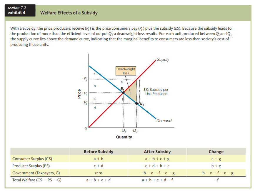
If taxes cause deadweight or welfare losses, do subsidies create welfare gains? For example, what if a government subsidy (paid by taxpayers) was provided in a particular market? Think of a subsidy as a negative tax. Before the subsidy, say the equilibrium price was $P_1$ and the equilibrium quantity was $Q_1$, as shown in Exhibit 4 . The consumer surplus is area $a+b$, and the producer surplus is area $\mathrm{c}+\mathrm{d}$. The sum of producer and consumer surpluses is maximized $(a+b+c+d)$, with no deadweight loss.

In Exhibit 4, we see that the subsidy lowers the price to the buyer to $P_B$ and increases the quantity exchanged to $Q_2$. The subsidy results in an increase in consumer surplus from area $a+b$ to area $a+b+c+g$, a gain of $c+g$. And producer surplus increases from area $c+d$ to area $c+d+b+e$, a gain of $b+e$. With gains in both consumer and producer surpluses, it looks like a gain in welfare, right? Not quite. Remember that the government is paying for this subsidy, and the cost to government (taxpayers) of the subsidy is area $b+\mathrm{e}+$ $\mathrm{f}+\mathrm{c}+\mathrm{g}$ (the subsidy per unit times the number of units subsidized). That is, the cost to government (taxpayers), area $\mathrm{b}+\mathrm{e}+\mathrm{f}+\mathrm{c}+\mathrm{g}$, is greater than the gains to consumers, $\mathrm{c}+\mathrm{g}$, and the gains to producers, $b+\mathrm{e}$, by area $\mathrm{f}$. Area $\mathrm{f}$ is the deadweight or welfare loss to society from the subsidy because it results in the production of more than the competitive market equilibrium, and the market value of that expansion to buyers is less than the marginal cost of producing that expansion to sellers. In short, the market overproduces relative to the efficient level of output, $Q_1$.

经济代写|宏观经济学代写Macroeconomics代考|Price Controls and Welfare Effects

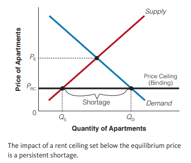
Historically, price ceilings have been set on a whole array of goods: apartments, auto insurance, electricity, cable television, food, gasoline, and many other products. What’s the impact of a price ceiling on buyers and sellers?

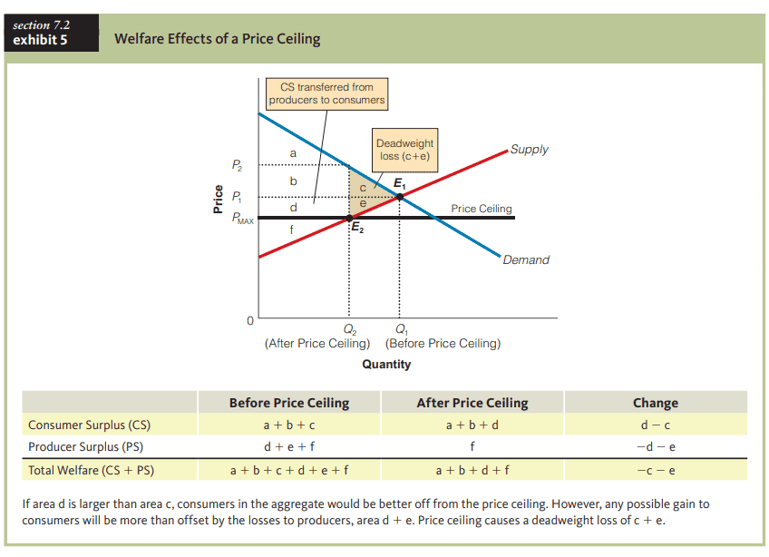
If a price ceiling (that is, a legally established maximum price) is binding and set below the equilibrium price at $P_{\operatorname{MAX}}$, the quantity demanded will be greater than the quantity supplied at that price, and a shortage will occur. At this price, buyers will compete for the limited supply, $Q_2$.

We can see the welfare effects of a price ceiling by observing the change in consumer and producer surpluses from the implementation of the price ceiling in Exhibit 5. Before the price ceiling, the buyer receives area $\mathrm{a}+\mathrm{b}+\mathrm{c}$ of consumer surplus at price $P_1$ and quantity $Q_1$. However, after the price ceiling is implemented at $P_{\text {MAX }}$, consumers can buy the good at a lower price but cannot buy as much as before (they can only buy $Q_2$ instead of $Q_1$ ). Because consumers can now buy $Q_2$ at a lower price, they gain area $\mathrm{d}$ of consumer surplus after the price ceiling. However, they lose area c of consumer surplus because they can only purchase $Q_2$ rather than $Q_1$ of output. Thus, the change in consumer surplus is $d-c$. In this case, area $d$ is larger than area $\mathrm{e}$ and area $\mathrm{c}$ and the consumer gains from the price ceiling.

The price the seller receives for $Q_2$ is $P_{\text {MAX }}$ (the ceiling price), so producer surplus falls from area $\mathrm{d}+\mathrm{e}+\mathrm{f}$ before the price ceiling to area $\mathrm{f}$ after the price ceiling, for a loss of area $\mathrm{d}+\mathrm{e}$. That is, any possible gain to consumers will be more than offset by the losses to producers. The price ceiling has caused a deadweight loss of area $\mathrm{c}+\mathrm{e}$. Notice, too, that area d, after the price ceiling, is a transfer of producer surplus to consumer surplus. That is, a transfer of surplus from sellers to buyers.

There is a deadweight loss because less is sold at $Q_2$ than at $Q_1$; and consumers value those units between $Q_2$ and $Q_1$ by more than it cost to produce them. For example, at $Q_2$, consumers will value the unit at $P_2$, which is much higher than it cost to produce it-the point on the supply curve at $Q_2$.

经济代写|宏观经济学代写Macroeconomics代考|ECON1120

宏观经济学代考

经济代写|宏观经济学代写Macroeconomics代考|The Welfare Effects of Subsidies

如果税收造成无谓负担或福利损失,那么补贴会创造福利收益吗?例如,如果某一特定市场提供了政府补贴(由纳税人支付)会怎样?可以把补贴想象成一种负税。在补贴前,假设均衡价格为$P_1$,均衡量为$Q_1$,如图4所示。消费者剩余为面积$a+b$,生产者剩余为面积$\ mathm {c}+\ mathm {d}$。生产者和消费者剩余的总和(a+b+c+d)最大化,没有无谓损失。

在表4中,我们看到补贴将对买方的价格降低到$P_B$,并将交换的数量增加到$Q_2$。补贴导致消费者剩余从区域$a+b$增加到区域$a+b+c+g$,增加$c+g$。生产者剩余从区域$c+d$增加到区域$c+d+b+e$,增加$b+e$。随着消费者和生产者盈余的增加,这看起来像是福利的增加,对吧?不完全是。记住,政府正在支付这项补贴,政府(纳税人)的补贴成本是面积$b+ $ $\ mathm {e}+$ $\ mathm {f}+ $ $\ mathm {c}+\ mathm {g}$(每单位的补贴乘以补贴的单位数量)。也就是说,政府(纳税人)的成本,面积$\ mathm {b}+\ mathm {e}+\ mathm {f}+\ mathm {c}+\ mathm {g}$,大于消费者的收益$\ mathm {c}+\ mathm {g}$,以及生产者的收益$b+\ mathm {e}$,按面积$\ mathm {f}$计算。面积{f}$是补贴给社会带来的无谓损失或福利损失,因为它导致生产超过竞争市场均衡,而这种扩张对买方的市场价值小于生产这种扩张对卖方的边际成本。简而言之,相对于产出的有效水平,Q_1,市场生产过剩。

经济代写|宏观经济学代写Macroeconomics代考|Price Controls and Welfare Effects

从历史上看,价格上限被设定在一系列商品上:公寓、汽车保险、电力、有线电视、食品、汽油和许多其他产品。价格上限对买家和卖家的影响是什么?

如果价格上限(即法律规定的最高价格)具有约束力,并设定在均衡价格$P_{\operatorname{MAX}}$以下,则需求数量将大于该价格下的供应量,并且将发生短缺。在这个价格下,买家将竞争有限的供应$Q_2$。

通过观察表5中价格上限实施后消费者和生产者剩余的变化,我们可以看到价格上限的福利效应。在价格上限之前,在价格$P_1$和数量$Q_1$时,购买者获得面积$\ mathm {a}+ $ mathm {b}+ $ mathm {c}$的消费者剩余。然而,在价格上限为$P_{\text {MAX}}$后,消费者可以以更低的价格购买商品,但不能像以前那样购买(他们只能购买$Q_2$而不是$Q_1$)。因为消费者现在可以以较低的价格购买$Q_2$,他们在价格上限后获得面积$\ mathm {d}$的消费者剩余。然而,他们损失了面积c的消费者剩余因为他们只能购买Q_2美元的产出而不是Q_1美元的产出。因此,消费者剩余的变化是$d- $ c。在这种情况下,面积$d$大于面积$\mathrm{e}$和面积$\mathrm{c}$,消费者从价格上限中获益。

卖方收到$Q_2$的价格为$P_{\text {MAX}}$(上限价格),因此生产者剩余从价格上限前的$\ mathm {d}+ $ mathm {e}+ $ mathm {f}$区域下降到价格上限后的$\ mathm {f}$区域,损失$\ mathm {d}+\ mathm {e}$区域。也就是说,消费者可能获得的任何收益都将被生产者的损失所抵消。价格上限造成了面积$\ mathm {c}+\ mathm {e}$的无谓损失。还要注意,在价格上限之后,面积d是生产者剩余向消费者剩余的转移。也就是说,盈余从卖方转移到买方。

这是无谓损失,因为Q_2美元的销售量少于Q_1美元;消费者对Q_2$和Q_1$之间的产品的价值高于生产成本。例如,在$Q_2$时,消费者对单位的估价为$P_2$,这比生产它的成本要高得多——供给曲线上的点为$Q_2$。

经济代写|宏观经济学代写Macroeconomics代考 请认准statistics-lab™

统计代写请认准statistics-lab™. statistics-lab™为您的留学生涯保驾护航。

金融工程代写

金融工程是使用数学技术来解决金融问题。金融工程使用计算机科学、统计学、经济学和应用数学领域的工具和知识来解决当前的金融问题,以及设计新的和创新的金融产品。

非参数统计代写

非参数统计指的是一种统计方法,其中不假设数据来自于由少数参数决定的规定模型;这种模型的例子包括正态分布模型和线性回归模型。

广义线性模型代考

广义线性模型(GLM)归属统计学领域,是一种应用灵活的线性回归模型。该模型允许因变量的偏差分布有除了正态分布之外的其它分布。

术语 广义线性模型(GLM)通常是指给定连续和/或分类预测因素的连续响应变量的常规线性回归模型。它包括多元线性回归,以及方差分析和方差分析(仅含固定效应)。

有限元方法代写

有限元方法(FEM)是一种流行的方法,用于数值解决工程和数学建模中出现的微分方程。典型的问题领域包括结构分析、传热、流体流动、质量运输和电磁势等传统领域。

有限元是一种通用的数值方法,用于解决两个或三个空间变量的偏微分方程(即一些边界值问题)。为了解决一个问题,有限元将一个大系统细分为更小、更简单的部分,称为有限元。这是通过在空间维度上的特定空间离散化来实现的,它是通过构建对象的网格来实现的:用于求解的数值域,它有有限数量的点。边界值问题的有限元方法表述最终导致一个代数方程组。该方法在域上对未知函数进行逼近。[1] 然后将模拟这些有限元的简单方程组合成一个更大的方程系统,以模拟整个问题。然后,有限元通过变化微积分使相关的误差函数最小化来逼近一个解决方案。

tatistics-lab作为专业的留学生服务机构,多年来已为美国、英国、加拿大、澳洲等留学热门地的学生提供专业的学术服务,包括但不限于Essay代写,Assignment代写,Dissertation代写,Report代写,小组作业代写,Proposal代写,Paper代写,Presentation代写,计算机作业代写,论文修改和润色,网课代做,exam代考等等。写作范围涵盖高中,本科,研究生等海外留学全阶段,辐射金融,经济学,会计学,审计学,管理学等全球99%专业科目。写作团队既有专业英语母语作者,也有海外名校硕博留学生,每位写作老师都拥有过硬的语言能力,专业的学科背景和学术写作经验。我们承诺100%原创,100%专业,100%准时,100%满意。

随机分析代写


随机微积分是数学的一个分支,对随机过程进行操作。它允许为随机过程的积分定义一个关于随机过程的一致的积分理论。这个领域是由日本数学家伊藤清在第二次世界大战期间创建并开始的。

时间序列分析代写

随机过程,是依赖于参数的一组随机变量的全体,参数通常是时间。 随机变量是随机现象的数量表现,其时间序列是一组按照时间发生先后顺序进行排列的数据点序列。通常一组时间序列的时间间隔为一恒定值(如1秒,5分钟,12小时,7天,1年),因此时间序列可以作为离散时间数据进行分析处理。研究时间序列数据的意义在于现实中,往往需要研究某个事物其随时间发展变化的规律。这就需要通过研究该事物过去发展的历史记录,以得到其自身发展的规律。

回归分析代写

多元回归分析渐进(Multiple Regression Analysis Asymptotics)属于计量经济学领域,主要是一种数学上的统计分析方法,可以分析复杂情况下各影响因素的数学关系,在自然科学、社会和经济学等多个领域内应用广泛。

MATLAB代写

MATLAB 是一种用于技术计算的高性能语言。它将计算、可视化和编程集成在一个易于使用的环境中,其中问题和解决方案以熟悉的数学符号表示。典型用途包括:数学和计算算法开发建模、仿真和原型制作数据分析、探索和可视化科学和工程图形应用程序开发,包括图形用户界面构建MATLAB 是一个交互式系统,其基本数据元素是一个不需要维度的数组。这使您可以解决许多技术计算问题,尤其是那些具有矩阵和向量公式的问题,而只需用 C 或 Fortran 等标量非交互式语言编写程序所需的时间的一小部分。MATLAB 名称代表矩阵实验室。MATLAB 最初的编写目的是提供对由 LINPACK 和 EISPACK 项目开发的矩阵软件的轻松访问,这两个项目共同代表了矩阵计算软件的最新技术。MATLAB 经过多年的发展,得到了许多用户的投入。在大学环境中,它是数学、工程和科学入门和高级课程的标准教学工具。在工业领域,MATLAB 是高效研究、开发和分析的首选工具。MATLAB 具有一系列称为工具箱的特定于应用程序的解决方案。对于大多数 MATLAB 用户来说非常重要,工具箱允许您学习应用专业技术。工具箱是 MATLAB 函数(M 文件)的综合集合,可扩展 MATLAB 环境以解决特定类别的问题。可用工具箱的领域包括信号处理、控制系统、神经网络、模糊逻辑、小波、仿真等。

R语言代写问卷设计与分析代写
PYTHON代写回归分析与线性模型代写
MATLAB代写方差分析与试验设计代写
STATA代写机器学习/统计学习代写
SPSS代写计量经济学代写
EVIEWS代写时间序列分析代写
EXCEL代写深度学习代写
SQL代写各种数据建模与可视化代写

经济代写|宏观经济学代写Macroeconomics代考|Consumer Surplus

如果你也在 怎样代写宏观经济学Macroeconomics 这个学科遇到相关的难题,请随时右上角联系我们的24/7代写客服。宏观经济学Macroeconomics对国家或地区经济整体行为的研究。它关注的是对整个经济事件的理解,如商品和服务的生产总量、失业水平和价格的一般行为。宏观经济学关注的是经济体的表现–经济产出、通货膨胀、利率和外汇兑换率以及国际收支的变化。减贫、社会公平和可持续增长只有在健全的货币和财政政策下才能实现。

宏观经济学Macroeconomics(来自希腊语前缀makro-,意思是 “大 “+经济学)是经济学的一个分支,处理整个经济体的表现、结构、行为和决策。例如,使用利率、税收和政府支出来调节经济的增长和稳定。这包括区域、国家和全球经济。根据经济学家Emi Nakamura和Jón Steinsson在2018年的评估,经济 “关于不同宏观经济政策的后果的证据仍然非常不完善,并受到严重批评。宏观经济学家研究的主题包括GDP(国内生产总值)、失业(包括失业率)、国民收入、价格指数、产出、消费、通货膨胀、储蓄、投资、能源、国际贸易和国际金融。

statistics-lab™ 为您的留学生涯保驾护航 在代写宏观经济学Macroeconomics方面已经树立了自己的口碑, 保证靠谱, 高质且原创的统计Statistics代写服务。我们的专家在代写宏观经济学Macroeconomics代写方面经验极为丰富,各种代写宏观经济学Macroeconomics相关的作业也就用不着说。

经济代写|宏观经济学代写Macroeconomics代考|Consumer Surplus

经济代写|宏观经济学代写Macroeconomics代考|Consumer Surplus

In a competitive market, consumers and producers buy and sell at the market equilibrium price. However, some consumers will be willing and able to pay more for the good than they have to. But they would never knowingly buy something that is worth less to them. That is, what a consumer actually pays for a unit of a good is usually less than the amount she is willing to pay. For example, would you be willing to pay more than the market price for a rope ladder to get out of a burning building? Would you be willing to pay more than the market price for a tank of gasoline if you had run out of gas on a desolate highway in the desert? Would you be willing to pay more than the market price for an anti-venom shot if you had been bitten by a rattlesnake? Consumer surplus is the monetary difference between the amount a consumer is willing and able to pay for an additional unit of a good and what the consumer actually paysthe market price. Consumer surplus for the whole market is the sum of all the individual consumer surpluses for those consumers who have purchased the good.

Suppose it is a hot day and iced tea is going for $\$ 1$ per glass, but Emily is willing to pay $\$ 4$ for the first glass (point a), $\$ 2$ for the second glass (point b), and $\$ 0.50$ for the third glass (point c), reflecting the law of demand. How much consumer surplus will Emily receive? First, it is important to note the general fact that if the consumer is a buyer of several units of a good, the earlier units will have greater marginal value and therefore create more consumer surplus because marginal willingness to pay falls as greater quantities are consumed in any period. In fact, you can think of the demand curve as a marginal benefit curve-the additional benefit derived from consuming one more unit. Notice in Exhibit 1 that Emily’s demand curve for iced tea has a step-like shape. This is demonstrated by Emily’s willingness to pay $\$ 4$ and $\$ 2$ successively for the first two glasses of iced tea. Thus, Emily will receive $\$ 3$ of consumer surplus for the first glass $(\$ 4-\$ 1)$ and $\$ 1$ of consumer surplus for the second glass $(\$ 2-\$ 1)$, for a total consumer surplus of $\$ 4$, as seen in Exhibit 1 . Emily will not be willing to purchase the third glass because her willingness to pay is less than its price $(\$ 0.50$ versus $\$ 1.00)$.
In Exhibit 2, we can easily measure the consumer surplus in the market by using a market demand curve rather than an individual demand curve. In short, the market consumer surplus is the area under the market demand curve and above the market price (the shaded area in Exhibit 2). The market for chocolate contains millions of potential buyers, so we will get a smooth demand curve. That is, each of the millions of potential buyers has their own willingness to pay. Because the demand curve represents the marginal benefits consumers receive from consuming an additional unit, we can conclude that all buyers of chocolate receive at least some consumer surplus in the market because the marginal benefit is greater than the market price-the shaded area in Exhibit 2 .

经济代写|宏观经济学代写Macroeconomics代考|Price Changes and Changes in Consumer Surplus

We may want to know how much consumers are hurt or helped when prices change. So let’s see what happens to consumer surplus when the price of a good rises or falls, when demand remains constant. Suppose that the price of your favorite beverage fell because of an increase in supply. Wouldn’t you feel better off? An increase in supply and a lower price will increase your consumer surplus for each unit you were already consuming and will also increase your consumer surplus from additional purchases at the lower price. Conversely, a decrease in supply and increase in price will lower your consumer surplus.

Exhibit 3 shows the gain in consumer surplus associated with a fall in the market price of pizza from $P_1$ to $P_2$. The fall in the market price leads to an increase in quantity demanded and an increase in consumer surplus. More specifically, consumer surplus increases from area $P_1 \mathrm{AB}$ to area $P_2 \mathrm{AC}$, for a gain in consumer surplus of $P_1 B C P_2$. The increase in consumer surplus has two parts. First, there is an increase in consumer surplus, because $Q_1$ can now be purchased at a lower price; this amount of additional consumer surplus is illustrated by area $P_1 \mathrm{BDP}_2$ in Exhibit 3. That is, these consumers would have purchased those pizzas at the original price of $P_1$, but now can purchase them at the new lower price of $P_2$. Second, the lower price makes it advantageous for buyers to expand their purchases from $Q_1$ to $Q_2$. The net benefit to buyers from expanding their consumption from $Q_1$ to $Q_2$ is illustrated by area BCD. That is, buyers would purchase those additional pizzas because the price was reduced. Similarly, if the market price of pizzas rose, the quantity demanded would fall. As a result, the two effects triggered by a decrease in price would increase consumer surplus, while an increase in price would decrease consumer surplus by $P_1 \mathrm{BCP}_2$.

In sum, consumer surplus measures the net gains buyers perceive that they receive, over and above the market price they must pay. So in this sense, it is a good measure of changes in economic well-being, if we assume that individuals make rational choices-self-betterment choices-and that individuals are the best judges of how much benefit they derive from goods and services.

经济代写|宏观经济学代写Macroeconomics代考|Consumer Surplus

宏观经济学代考

经济代写|宏观经济学代写Macroeconomics代考|Consumer Surplus

在竞争市场中,消费者和生产者以市场均衡价格进行买卖。然而,一些消费者愿意并且有能力为这些商品支付比他们必须支付的更多的钱。但他们永远不会故意购买对他们来说价值较低的东西。也就是说,消费者为一单位商品实际支付的价格通常低于她愿意支付的价格。例如,你愿意花比市场价更高的价格买一个绳梯从着火的大楼里出来吗?如果你在荒凉的沙漠公路上没油了,你愿意花比市场价更高的价钱买一箱汽油吗?如果你被响尾蛇咬了,你会愿意花比市场价更高的价钱去打一针抗蛇毒疫苗吗?消费者剩余是消费者愿意和能够为一单位额外商品支付的金额与消费者实际支付的市场价格之间的货币差额。整个市场的消费者剩余是购买了该商品的消费者的所有个人消费者剩余的总和。

假设天气很热,冰茶的价格是每杯1美元,但艾米丽愿意花4美元买第一杯(a点),花2美元买第二杯(b点),花0.50美元买第三杯(c点),这反映了需求定律。艾米丽会得到多少消费者剩余?首先,重要的是要注意这样一个普遍的事实,即如果消费者是一种商品的几个单位的购买者,那么较早的单位将具有更大的边际价值,从而产生更多的消费者剩余,因为边际支付意愿随着任何时期消费数量的增加而下降。事实上,你可以把需求曲线看作边际效益曲线——多消费一单位产品所产生的额外效益。注意,在图表1中,艾米丽对冰茶的需求曲线呈阶梯状。艾米丽愿意为前两杯冰茶连续支付$ $ 4和$ $ 2就证明了这一点。因此,艾米丽将从第一杯酒中获得$ $ $ 3的消费者剩余$ $($ $ 4- $ $ 1)$,从第二杯酒中获得$ $ $ 1的消费者剩余$ $ $($ $ 2- $ $ 1)$,总的消费者剩余$ $ $ 4,如表1所示。艾米丽不愿意购买第三个杯子,因为她的支付意愿低于它的价格(0.50美元对1.00美元)。
在表2中,我们可以很容易地通过使用市场需求曲线而不是个人需求曲线来衡量市场中的消费者剩余。简而言之,市场消费者剩余是市场需求曲线下方和市场价格上方的面积(图2中的阴影区域)。巧克力市场包含数百万潜在买家,因此我们将得到一条平滑的需求曲线。也就是说,数百万潜在买家中的每个人都有自己的支付意愿。因为需求曲线代表消费者从额外消费一单位中获得的边际效益,我们可以得出结论,所有巧克力的购买者在市场上至少获得了一些消费者剩余,因为边际效益大于市场价格(图2中的阴影区域)。

经济代写|宏观经济学代写Macroeconomics代考|Price Changes and Changes in Consumer Surplus

我们可能想知道价格变化对消费者的伤害或帮助有多大。看看需求保持不变时,商品价格上升或下降时,消费者剩余会怎样。假设你最喜欢的饮料的价格因为供给的增加而下降。你会不会感觉好些?供给的增加和较低的价格会增加你已经消费的每单位的消费者剩余,也会增加你在较低价格下额外购买的消费者剩余。相反,供给的减少和价格的增加会降低消费者剩余。

图3显示了消费者剩余的增加与披萨市场价格从$P_1$下降到$P_2$有关。市场价格的下跌导致需求量的增加和消费者剩余的增加。更具体地说,消费者剩余从面积$P_1 \ mathm {AB}$增加到面积$P_2 \ mathm {AC}$,消费者剩余增加$P_1 B C P_2$。消费者剩余的增加有两个部分。首先,消费者剩余增加,因为Q_1美元现在可以以更低的价格购买;这个数量的额外消费者剩余在表3中用面积$P_1 \ mathm {BDP}_2$表示。也就是说,这些消费者会以原价$P_1$购买这些披萨,但现在可以以新的较低价格$P_2$购买。其次,较低的价格有利于买家将购买金额从$Q_1$扩大到$Q_2$。购买者将消费从$Q_1$扩大到$Q_2$的净收益用面积BCD表示。也就是说,买家会因为价格降低而购买那些额外的披萨。同样,如果披萨的市场价格上涨,需求量就会下降。结果表明,价格下降引起的两种效应均使消费者剩余增加,而价格上涨则使消费者剩余减少$P_1 \ mathm {BCP}_2$。

总而言之,消费者剩余衡量的是购买者认为他们获得的净收益,高于他们必须支付的市场价格。因此,从这个意义上说,如果我们假设个人做出理性选择——自我改善的选择——并且个人是他们从商品和服务中获得多少利益的最佳判断者,那么它是衡量经济福祉变化的一个很好的指标。

经济代写|宏观经济学代写Macroeconomics代考 请认准statistics-lab™

统计代写请认准statistics-lab™. statistics-lab™为您的留学生涯保驾护航。

金融工程代写

金融工程是使用数学技术来解决金融问题。金融工程使用计算机科学、统计学、经济学和应用数学领域的工具和知识来解决当前的金融问题,以及设计新的和创新的金融产品。

非参数统计代写

非参数统计指的是一种统计方法,其中不假设数据来自于由少数参数决定的规定模型;这种模型的例子包括正态分布模型和线性回归模型。

广义线性模型代考

广义线性模型(GLM)归属统计学领域,是一种应用灵活的线性回归模型。该模型允许因变量的偏差分布有除了正态分布之外的其它分布。

术语 广义线性模型(GLM)通常是指给定连续和/或分类预测因素的连续响应变量的常规线性回归模型。它包括多元线性回归,以及方差分析和方差分析(仅含固定效应)。

有限元方法代写

有限元方法(FEM)是一种流行的方法,用于数值解决工程和数学建模中出现的微分方程。典型的问题领域包括结构分析、传热、流体流动、质量运输和电磁势等传统领域。

有限元是一种通用的数值方法,用于解决两个或三个空间变量的偏微分方程(即一些边界值问题)。为了解决一个问题,有限元将一个大系统细分为更小、更简单的部分,称为有限元。这是通过在空间维度上的特定空间离散化来实现的,它是通过构建对象的网格来实现的:用于求解的数值域,它有有限数量的点。边界值问题的有限元方法表述最终导致一个代数方程组。该方法在域上对未知函数进行逼近。[1] 然后将模拟这些有限元的简单方程组合成一个更大的方程系统,以模拟整个问题。然后,有限元通过变化微积分使相关的误差函数最小化来逼近一个解决方案。

tatistics-lab作为专业的留学生服务机构,多年来已为美国、英国、加拿大、澳洲等留学热门地的学生提供专业的学术服务,包括但不限于Essay代写,Assignment代写,Dissertation代写,Report代写,小组作业代写,Proposal代写,Paper代写,Presentation代写,计算机作业代写,论文修改和润色,网课代做,exam代考等等。写作范围涵盖高中,本科,研究生等海外留学全阶段,辐射金融,经济学,会计学,审计学,管理学等全球99%专业科目。写作团队既有专业英语母语作者,也有海外名校硕博留学生,每位写作老师都拥有过硬的语言能力,专业的学科背景和学术写作经验。我们承诺100%原创,100%专业,100%准时,100%满意。

随机分析代写


随机微积分是数学的一个分支,对随机过程进行操作。它允许为随机过程的积分定义一个关于随机过程的一致的积分理论。这个领域是由日本数学家伊藤清在第二次世界大战期间创建并开始的。

时间序列分析代写

随机过程,是依赖于参数的一组随机变量的全体,参数通常是时间。 随机变量是随机现象的数量表现,其时间序列是一组按照时间发生先后顺序进行排列的数据点序列。通常一组时间序列的时间间隔为一恒定值(如1秒,5分钟,12小时,7天,1年),因此时间序列可以作为离散时间数据进行分析处理。研究时间序列数据的意义在于现实中,往往需要研究某个事物其随时间发展变化的规律。这就需要通过研究该事物过去发展的历史记录,以得到其自身发展的规律。

回归分析代写

多元回归分析渐进(Multiple Regression Analysis Asymptotics)属于计量经济学领域,主要是一种数学上的统计分析方法,可以分析复杂情况下各影响因素的数学关系,在自然科学、社会和经济学等多个领域内应用广泛。

MATLAB代写

MATLAB 是一种用于技术计算的高性能语言。它将计算、可视化和编程集成在一个易于使用的环境中,其中问题和解决方案以熟悉的数学符号表示。典型用途包括:数学和计算算法开发建模、仿真和原型制作数据分析、探索和可视化科学和工程图形应用程序开发,包括图形用户界面构建MATLAB 是一个交互式系统,其基本数据元素是一个不需要维度的数组。这使您可以解决许多技术计算问题,尤其是那些具有矩阵和向量公式的问题,而只需用 C 或 Fortran 等标量非交互式语言编写程序所需的时间的一小部分。MATLAB 名称代表矩阵实验室。MATLAB 最初的编写目的是提供对由 LINPACK 和 EISPACK 项目开发的矩阵软件的轻松访问,这两个项目共同代表了矩阵计算软件的最新技术。MATLAB 经过多年的发展,得到了许多用户的投入。在大学环境中,它是数学、工程和科学入门和高级课程的标准教学工具。在工业领域,MATLAB 是高效研究、开发和分析的首选工具。MATLAB 具有一系列称为工具箱的特定于应用程序的解决方案。对于大多数 MATLAB 用户来说非常重要,工具箱允许您学习应用专业技术。工具箱是 MATLAB 函数(M 文件)的综合集合,可扩展 MATLAB 环境以解决特定类别的问题。可用工具箱的领域包括信号处理、控制系统、神经网络、模糊逻辑、小波、仿真等。

R语言代写问卷设计与分析代写
PYTHON代写回归分析与线性模型代写
MATLAB代写方差分析与试验设计代写
STATA代写机器学习/统计学习代写
SPSS代写计量经济学代写
EVIEWS代写时间序列分析代写
EXCEL代写深度学习代写
SQL代写各种数据建模与可视化代写

经济代写|宏观经济学代写Macroeconomics代考|How Does the Price Elasticity of Demand Impact Total Revenue?

如果你也在 怎样代写宏观经济学Macroeconomics 这个学科遇到相关的难题,请随时右上角联系我们的24/7代写客服。宏观经济学Macroeconomics对国家或地区经济整体行为的研究。它关注的是对整个经济事件的理解,如商品和服务的生产总量、失业水平和价格的一般行为。宏观经济学关注的是经济体的表现–经济产出、通货膨胀、利率和外汇兑换率以及国际收支的变化。减贫、社会公平和可持续增长只有在健全的货币和财政政策下才能实现。

宏观经济学Macroeconomics(来自希腊语前缀makro-,意思是 “大 “+经济学)是经济学的一个分支,处理整个经济体的表现、结构、行为和决策。例如,使用利率、税收和政府支出来调节经济的增长和稳定。这包括区域、国家和全球经济。根据经济学家Emi Nakamura和Jón Steinsson在2018年的评估,经济 “关于不同宏观经济政策的后果的证据仍然非常不完善,并受到严重批评。宏观经济学家研究的主题包括GDP(国内生产总值)、失业(包括失业率)、国民收入、价格指数、产出、消费、通货膨胀、储蓄、投资、能源、国际贸易和国际金融。

statistics-lab™ 为您的留学生涯保驾护航 在代写宏观经济学Macroeconomics方面已经树立了自己的口碑, 保证靠谱, 高质且原创的统计Statistics代写服务。我们的专家在代写宏观经济学Macroeconomics代写方面经验极为丰富,各种代写宏观经济学Macroeconomics相关的作业也就用不着说。

经济代写|宏观经济学代写Macroeconomics代考|How Does the Price Elasticity of Demand Impact Total Revenue?

经济代写|宏观经济学代写Macroeconomics代考|Proportion of Income Spent on the Good

The price elasticity of demand for a good also has implications for total revenue. Total revenue (TR) is the amount sellers receive for a good or service. Total revenue is simply the price of the good $(P)$ times the quantity of the good sold $(Q): T R=P \times Q$. The elasticity of demand will help to predict how changes in the price will impact total revenue earned by the producer for selling the good. Let’s see how this works.

In Exhibit 1 , we see that when the demand is price elastic $\left(E_{\mathrm{D}}>1\right)$, total revenues will rise as the price declines, because the percentage increase in the quantity demanded is greater than the percentage reduction in price. For example, if the price of a good is cut in half (say from $\$ 10$ to $\$ 5$ ) and the quantity demanded more than doubles (say from 40 to 100 ), total revenue will rise from $\$ 400(\$ 10 \times 40=\$ 400)$ to $\$ 500(\$ 5 \times 100=\$ 500)$. Equivalently, if the price rises from $\$ 5$ to $\$ 10$ and the quantity demanded falls from 100 to 40 units, then total revenue will fall from $\$ 500$ to $\$ 400$. As this example illustrates, if the demand curve is relatively elastic, total revenue will vary inversely with a price change.

You can see from the following what happens to total revenue when demand is price elastic. (Note: The size of the price and quantity arrows represents the size of the percentage changes.)
When Demand Is Price Elastic
$$
\downarrow T R=\uparrow P \times \downarrow Q
$$
or
$$
\uparrow T R=\downarrow P \times \uparrow Q
$$
On the other hand, if demand for a good is relatively inelastic $\left(E_{\mathrm{D}}<1\right)$, the total revenue will be lower at lower prices than at higher prices because a given price reduction will be accompanied by a proportionately smaller increase in quantity demanded. For example, as shown in Exhibit 2, if the price of a good is cut (say from $\$ 10$ to $\$ 5$ ) and the quantity demanded less than doubles (say it increases from 30 to 40 ), then total revenue will fall from $\$ 300(\$ 10 \times 30=\$ 300)$ to $\$ 200(\$ 5 \times 40=\$ 200)$. Equivalently, if the price increases from $\$ 5$ to $\$ 10$ and the quantity demanded falls from 40 to 30 , total revenue will increase from $\$ 200$ to $\$ 300$. That is, if the demand curve is inelastic, total revenue will vary directly with a price change.
When Demand Is Price Inelastic
$$
\begin{aligned}
\uparrow T R= & \uparrow P \times \downarrow Q \
& \text { or } \
\downarrow T R= & \downarrow P \times \uparrow Q
\end{aligned}
$$
or
In this case, the “net” effect on total revenue is reversed but easy to see. (Again, the size of the price and quantity arrows represents the size of the percentage changes.)

经济代写|宏观经济学代写Macroeconomics代考|Price Elasticity Changes along a Linear Demand Curve

As already shown (Section 6.1, Exhibit 1), the slopes of demand curves can be used to estimate their relative elasticities of demand: The steeper one demand curve is relative to another, the more inelastic it is relative to the other. However, except for the extreme cases of perfectly elastic and perfectly inelastic curves, great care must be taken when trying to estimate the degree of elasticity of one demand curve from its slope. In fact, as we will soon see, a straight-line demand curve with a constant slope will change elasticity continuously as you move up or down it. It is because the slope is the ratio of changes in the two variables (price and quantity) while the elasticity is the ratio of percentage changes in the two variables.

We can easily demonstrate that the elasticity of demand varies along a linear demand curve by using what we already know about the interrelationship between price and total revenue.

Exhibit 4 shows a linear (constant slope) demand curve. In Exhibit 4(a), we see that when the price falls on the upper half of the demand curve from $P_1$ to $P_2$, and quantity demanded increases from $Q_1$ to $Q_2$, total revenue increases. That is, the new area of total revenue $($ area $b+c$ ) is larger than the old area of total revenue (area $a+b)$. It is also true that if price increased in this region (from $P_2$ to $P_1$ ), total revenue would fall because $\mathrm{b}+\mathrm{c}$ is greater than $\mathrm{a}+\mathrm{b}$.

In this region of the demand curve, then, there is a negative relationship between price and total revenue. As we discussed earlier, this is characteristic of an elastic demand curve $\left(E_{\mathrm{D}}>1\right)$.
Exhibit 4(b) illustrates what happens to total revenue on the lower half of the same demand curve. When the price falls from $P_3$ to $P_4$ and the quantity demanded increases from $Q_3$ to $Q_4$, total revenue actually decreases because the new area of total revenue (area $\mathrm{e}+\mathrm{f}$ ) is less than the old area of total revenue (area $\mathrm{d}+\mathrm{e}$ ). Likewise, it is clear that an increase in price from $P_4$ to $P_3$ would increase total revenue. In this case, there is a positive relationship between price and total revenue, which, as we discussed, is characteristic of an inelastic demand curve $\left(E_{\mathrm{D}}<1\right)$. Together, parts (a) and (b) of Exhibit 4 illustrate that, although the slope remains constant, the elasticity of a linear demand curve changes along the length of the curve-from relatively elastic at higher price ranges to relatively inelastic at lower price ranges.

经济代写|宏观经济学代写Macroeconomics代考|How Does the Price Elasticity of Demand Impact Total Revenue?

宏观经济学代考

经济代写|宏观经济学代写Macroeconomics代考|Proportion of Income Spent on the Good

商品需求的价格弹性也会影响总收入。总收益(TR)是卖方从商品或服务中获得的金额。总收入就是商品的价格$(P)$乘以商品的销售量$(Q): T R=P \times Q$。需求弹性将有助于预测价格的变化将如何影响生产者销售商品所获得的总收入。让我们看看它是如何工作的。

在表1中,我们看到,当需求具有价格弹性$\left(E_{\mathrm{D}}>1\right)$时,总收益将随着价格下降而上升,因为需求量增加的百分比大于价格下降的百分比。例如,如果一种商品的价格减半(比如从$\$ 10$降至$\$ 5$),而需求量增加一倍以上(比如从40降至100),总收入将从$\$ 400(\$ 10 \times 40=\$ 400)$上升至$\$ 500(\$ 5 \times 100=\$ 500)$。同样地,如果价格从$\$ 5$上升到$\$ 10$,需求量从100下降到40,那么总收益将从$\$ 500$下降到$\$ 400$。如本例所示,如果需求曲线是相对弹性的,总收入将与价格变化成反比。

从下图可以看出,当需求具有价格弹性时,总收入的变化情况。(注:价格和数量箭头的大小代表百分比变化的大小。)
当需求具有价格弹性时
$$
\downarrow T R=\uparrow P \times \downarrow Q
$$

$$
\uparrow T R=\downarrow P \times \uparrow Q
$$
另一方面,如果对一种商品的需求相对缺乏弹性$\left(E_{\mathrm{D}}<1\right)$,则总收益在价格较低时将低于价格较高时,因为给定的价格降低将伴随着按比例较小的需求量增加。例如,如图2所示,如果一种商品的价格降低(比如从$\$ 10$降至$\$ 5$),而需求量增加一倍以下(比如从30增加到40),那么总收入将从$\$ 300(\$ 10 \times 30=\$ 300)$降至$\$ 200(\$ 5 \times 40=\$ 200)$。同样,如果价格从$\$ 5$上升到$\$ 10$,需求量从40下降到30,总收益将从$\$ 200$上升到$\$ 300$。也就是说,如果需求曲线是非弹性的,总收入将直接随价格变化而变化。
当需求价格无弹性时
$$
\begin{aligned}
\uparrow T R= & \uparrow P \times \downarrow Q \
& \text { or } \
\downarrow T R= & \downarrow P \times \uparrow Q
\end{aligned}
$$

在这种情况下,对总收入的“净”影响是相反的,但很容易看到。(同样,价格和数量箭头的大小表示百分比变化的大小。)

经济代写|宏观经济学代写Macroeconomics代考|Price Elasticity Changes along a Linear Demand Curve

如前所述(第6.1节,表1),需求曲线的斜率可以用来估计需求的相对弹性:一条需求曲线相对于另一条需求曲线越陡峭,它相对于另一条需求曲线的弹性就越小。然而,除了完全弹性曲线和完全非弹性曲线的极端情况外,在试图从一条需求曲线的斜率估计其弹性程度时,必须非常小心。事实上,我们很快就会看到,斜率为常数的直线需求曲线会随着上下移动而不断改变弹性。这是因为斜率是两个变量(价格和数量)变化的比率,而弹性是两个变量变化百分比的比率。

通过使用我们已经知道的价格和总收入之间的相互关系,我们可以很容易地证明需求弹性沿着线性需求曲线变化。

图4显示了一条线性(斜率恒定)需求曲线。在图4(a)中,我们看到,当价格在需求曲线的上半部分从$P_1$下降到$P_2$时,需求量从$Q_1$增加到$Q_2$,总收入增加。也就是说,总收入的新区域$(区域$b+c$)大于总收入的旧区域$(区域$a+b)$。同样,如果该区域的价格上涨(从$P_2$到$P_1$),总收益将下降,因为$\ mathm {b}+\ mathm {c}$大于$\ mathm {a}+\ mathm {b}$。

因此,在需求曲线的这个区域,价格和总收入之间存在负相关关系。正如我们前面所讨论的,这是弹性需求曲线$\left(E_{\ mathm {D}}>1\right)$的特征。
图4(b)展示了同一需求曲线下半部分的总收入。当价格从$P_3$下降到$P_4$,需求量从$Q_3$增加到$Q_4$时,总收入实际上减少了,因为总收入的新区域($\ mathm {e}+\ mathm {f}$)小于总收入的旧区域($\ mathm {d}+\ mathm {e}$)。同样,很明显,价格从$P_4$增加到$P_3$会增加总收入。在这种情况下,价格和总收入之间存在正关系,正如我们所讨论的,这是非弹性需求曲线$\left(E_{\ mathm {D}}<1\right)$的特征。图4的(a)和(b)部分共同说明,尽管斜率保持不变,但线性需求曲线的弹性沿着曲线的长度变化——从较高价格区间的相对弹性到较低价格区间的相对无弹性。

经济代写|宏观经济学代写Macroeconomics代考 请认准statistics-lab™

统计代写请认准statistics-lab™. statistics-lab™为您的留学生涯保驾护航。

金融工程代写

金融工程是使用数学技术来解决金融问题。金融工程使用计算机科学、统计学、经济学和应用数学领域的工具和知识来解决当前的金融问题,以及设计新的和创新的金融产品。

非参数统计代写

非参数统计指的是一种统计方法,其中不假设数据来自于由少数参数决定的规定模型;这种模型的例子包括正态分布模型和线性回归模型。

广义线性模型代考

广义线性模型(GLM)归属统计学领域,是一种应用灵活的线性回归模型。该模型允许因变量的偏差分布有除了正态分布之外的其它分布。

术语 广义线性模型(GLM)通常是指给定连续和/或分类预测因素的连续响应变量的常规线性回归模型。它包括多元线性回归,以及方差分析和方差分析(仅含固定效应)。

有限元方法代写

有限元方法(FEM)是一种流行的方法,用于数值解决工程和数学建模中出现的微分方程。典型的问题领域包括结构分析、传热、流体流动、质量运输和电磁势等传统领域。

有限元是一种通用的数值方法,用于解决两个或三个空间变量的偏微分方程(即一些边界值问题)。为了解决一个问题,有限元将一个大系统细分为更小、更简单的部分,称为有限元。这是通过在空间维度上的特定空间离散化来实现的,它是通过构建对象的网格来实现的:用于求解的数值域,它有有限数量的点。边界值问题的有限元方法表述最终导致一个代数方程组。该方法在域上对未知函数进行逼近。[1] 然后将模拟这些有限元的简单方程组合成一个更大的方程系统,以模拟整个问题。然后,有限元通过变化微积分使相关的误差函数最小化来逼近一个解决方案。

tatistics-lab作为专业的留学生服务机构,多年来已为美国、英国、加拿大、澳洲等留学热门地的学生提供专业的学术服务,包括但不限于Essay代写,Assignment代写,Dissertation代写,Report代写,小组作业代写,Proposal代写,Paper代写,Presentation代写,计算机作业代写,论文修改和润色,网课代做,exam代考等等。写作范围涵盖高中,本科,研究生等海外留学全阶段,辐射金融,经济学,会计学,审计学,管理学等全球99%专业科目。写作团队既有专业英语母语作者,也有海外名校硕博留学生,每位写作老师都拥有过硬的语言能力,专业的学科背景和学术写作经验。我们承诺100%原创,100%专业,100%准时,100%满意。

随机分析代写


随机微积分是数学的一个分支,对随机过程进行操作。它允许为随机过程的积分定义一个关于随机过程的一致的积分理论。这个领域是由日本数学家伊藤清在第二次世界大战期间创建并开始的。

时间序列分析代写

随机过程,是依赖于参数的一组随机变量的全体,参数通常是时间。 随机变量是随机现象的数量表现,其时间序列是一组按照时间发生先后顺序进行排列的数据点序列。通常一组时间序列的时间间隔为一恒定值(如1秒,5分钟,12小时,7天,1年),因此时间序列可以作为离散时间数据进行分析处理。研究时间序列数据的意义在于现实中,往往需要研究某个事物其随时间发展变化的规律。这就需要通过研究该事物过去发展的历史记录,以得到其自身发展的规律。

回归分析代写

多元回归分析渐进(Multiple Regression Analysis Asymptotics)属于计量经济学领域,主要是一种数学上的统计分析方法,可以分析复杂情况下各影响因素的数学关系,在自然科学、社会和经济学等多个领域内应用广泛。

MATLAB代写

MATLAB 是一种用于技术计算的高性能语言。它将计算、可视化和编程集成在一个易于使用的环境中,其中问题和解决方案以熟悉的数学符号表示。典型用途包括:数学和计算算法开发建模、仿真和原型制作数据分析、探索和可视化科学和工程图形应用程序开发,包括图形用户界面构建MATLAB 是一个交互式系统,其基本数据元素是一个不需要维度的数组。这使您可以解决许多技术计算问题,尤其是那些具有矩阵和向量公式的问题,而只需用 C 或 Fortran 等标量非交互式语言编写程序所需的时间的一小部分。MATLAB 名称代表矩阵实验室。MATLAB 最初的编写目的是提供对由 LINPACK 和 EISPACK 项目开发的矩阵软件的轻松访问,这两个项目共同代表了矩阵计算软件的最新技术。MATLAB 经过多年的发展,得到了许多用户的投入。在大学环境中,它是数学、工程和科学入门和高级课程的标准教学工具。在工业领域,MATLAB 是高效研究、开发和分析的首选工具。MATLAB 具有一系列称为工具箱的特定于应用程序的解决方案。对于大多数 MATLAB 用户来说非常重要,工具箱允许您学习应用专业技术。工具箱是 MATLAB 函数(M 文件)的综合集合,可扩展 MATLAB 环境以解决特定类别的问题。可用工具箱的领域包括信号处理、控制系统、神经网络、模糊逻辑、小波、仿真等。

R语言代写问卷设计与分析代写
PYTHON代写回归分析与线性模型代写
MATLAB代写方差分析与试验设计代写
STATA代写机器学习/统计学习代写
SPSS代写计量经济学代写
EVIEWS代写时间序列分析代写
EXCEL代写深度学习代写
SQL代写各种数据建模与可视化代写

经济代写|宏观经济学代写Macroeconomics代考|Price Controls

如果你也在 怎样代写宏观经济学Macroeconomics 这个学科遇到相关的难题,请随时右上角联系我们的24/7代写客服。宏观经济学Macroeconomics对国家或地区经济整体行为的研究。它关注的是对整个经济事件的理解,如商品和服务的生产总量、失业水平和价格的一般行为。宏观经济学关注的是经济体的表现–经济产出、通货膨胀、利率和外汇兑换率以及国际收支的变化。减贫、社会公平和可持续增长只有在健全的货币和财政政策下才能实现。

宏观经济学Macroeconomics(来自希腊语前缀makro-,意思是 “大 “+经济学)是经济学的一个分支,处理整个经济体的表现、结构、行为和决策。例如,使用利率、税收和政府支出来调节经济的增长和稳定。这包括区域、国家和全球经济。根据经济学家Emi Nakamura和Jón Steinsson在2018年的评估,经济 “关于不同宏观经济政策的后果的证据仍然非常不完善,并受到严重批评。宏观经济学家研究的主题包括GDP(国内生产总值)、失业(包括失业率)、国民收入、价格指数、产出、消费、通货膨胀、储蓄、投资、能源、国际贸易和国际金融。

statistics-lab™ 为您的留学生涯保驾护航 在代写宏观经济学Macroeconomics方面已经树立了自己的口碑, 保证靠谱, 高质且原创的统计Statistics代写服务。我们的专家在代写宏观经济学Macroeconomics代写方面经验极为丰富,各种代写宏观经济学Macroeconomics相关的作业也就用不着说。

经济代写|宏观经济学代写Macroeconomics代考|Price Controls

经济代写|宏观经济学代写Macroeconomics代考|Price Controls

Although non-equilibrium prices can occur naturally in the private sector, reflecting uncertainty, they seldom last for long. Governments, however, may impose non-equilibrium prices for significant periods. Price controls involve the use of the power of the state to establish prices different from the equilibrium prices that would otherwise prevail. The motivations for price controls vary with the market under consideration. For example, a price ceiling, a legal maximum price, is often set for goods deemed important to low-income households, such as housing. Or a price floor, a legal minimum price, may be set on wages because wages are the primary source of income for most people.

Price controls are not always implemented by the federal government. Local governments (and more rarely, private companies) can and do impose local price controls. One fairly wellknown example is rent control. The inflation of the late 1970 s meant rapidly rising rents; some communities, such as Santa Monica, California, decided to do something about it. In response, they limited how much landlords could charge for rental housing.

Price Ceilings: Rent Controls
Rent control experiences can be found in many cities across the country. San Francisco, Berkeley, and New York City all have had some form of rent control. Although the rules may vary from city to city and over time, generally the price (or rent) of an apartment remains fixed over the tenure of an occupant, except for allowable annual increases tied to the cost of living or some other price index. When an occupant moves out, the owners can usually, but not always, raise the rent to a near-market level for the next occupant. The controlled rents for existing occupants, however, are generally well below market rental rates.

Results of Rent Controls
Most people living in rent-controlled apartments are getting a good deal, one that they would lose by moving as their family circumstances or income changes. Tenants thus are reluctant to give up their governmentally granted right to a below-market-rent apartment. In addition, because the rents received by landlords are constrained and below market levels, the rate of return (roughly, the profit) on housing investments falls compared with that on other forms of real estate not subject to rent controls, such as office rents or mortgage payments on condominiums. Hence, the incentive to construct new housing is reduced.

Furthermore, when landlords are limited in the rents they can charge, they have little incentive to improve or upgrade apartments-by putting in new kitchen appliances or new carpeting, for instance. In fact, rent controls give landlords some incentive to avoid routine maintenance, thereby lowering the cost of apartment ownership to a figure approximating the controlled rental price, although the quality of the housing stock will deteriorate over time. Another impact of rent controls is that they promote housing discrimination. Where rent controls do not exist, prejudiced landlords might willingly rent to people they believe are undesirable simply because the undesirables are the only ones willing to pay the requested rents (and the landlords are not willing to lower their rents substantially to get desirable renters because of the possible loss of thousands of dollars in income). With rent controls, each rent-controlled apartment is likely to attract many possible renters, some desirable and some undesirable as judged by the landlord, simply because the rent is at a below-equilibrium price. Landlords can indulge in their “taste” for discrimination without any additional financial loss beyond that required by the controls. Consequently, they will be more likely to choose to rent to desirable people, perhaps a family without children or pets, rather than to undesirable ones, perhaps a family with lower income and so a greater risk of nonpayment.

Exhibit 1 shows the impact of rent controls. If the price ceiling $\left(P_{\mathrm{RC}}\right)$ is set below the equilibrium price $\left(P_{\mathrm{E}}\right)$, consumers are willing to buy $Q_{\mathrm{D}}$, but producers are only willing to supply $Q_s$. The rent control policy will therefore create a persistent shortage, the difference between $Q_D$ and $Q_s$.

经济代写|宏观经济学代写Macroeconomics代考|Price Floors: The Minimum Wage

The argument for a minimum wage is simple: Existing wages for workers in some types of labor markets do not allow for a very high standard of living, and a minimum wage allows those workers to live better than before. Ever since 1938, when the first minimum wage was established (at 25 cents per hour), the federal government has, by legislation, made it illegal to pay most workers an amount below the current legislated minimum wage. In 2014 , the federal minimum wage was set at $\$ 7.25$. A number of states also have minimum-wage laws. In cases where an employee is subject to both state and federal minimum-wage laws, the employee is entitled to the higher minimum wage.

Let’s examine graphically the impact of a minimum wage on low-skilled workers. In Exhibit 2, suppose the government sets the minimum wage, $W_{M I N}$, above the market equilibrium wage, $W_{\mathrm{E}}$. In Exhibit 2, we see that the price floor is binding. That is, there is a surplus of low-skilled workers at $W_{\text {MIN }}$ because the quantity of labor supplied is greater than the quantity of labor demanded. The reason for the surplus of low-skilled workers (unemployment) at $W_{\mathrm{MIN}}$ is that more people are willing to work than employers are willing and able to hire.
Notice that not everyone loses from a minimum wage. Workers who continue to hold jobs have higher incomesthose between 0 and $Q_D$ in Exhibit 2. However, many lowskilled workers suffer from a minimum wage-those between $Q_D$ and $Q_S$ in Exhibit 2-because they either lose their jobs or are unable to get them in the first place. Although studies disagree somewhat on the precise magnitudes, they largely agree that minimum-wage laws do create some unemployment and that the unemployment is concentrated among teenagers-the least-experienced and least-skilled members of the labor force. Many teenagers are willing to accept the lower wage in exchange for on-the-job training. In fact, some college students accept non-paying intern jobs for the experience. Minimum-wage laws do not apply to internships, and if they did, many of those jobs might not exist.

经济代写|宏观经济学代写Macroeconomics代考|Price Controls

宏观经济学代考

经济代写|宏观经济学代写Macroeconomics代考|Price Controls

尽管非均衡价格可以在私营部门自然出现,反映出不确定性,但它们很少持续很长时间。然而,政府可能在相当长的时期内强制实行非均衡价格。价格控制包括使用国家权力来制定不同于均衡价格的价格。价格管制的动机因所考虑的市场而异。例如,对于住房等被认为对低收入家庭很重要的商品,通常会设定价格上限,即法定最高价格。由于工资是大多数人的主要收入来源,因此可以对工资设定最低价格。

价格管制并不总是由联邦政府实施。地方政府(以及更罕见的私营企业)能够而且确实实施了地方价格控制。一个相当著名的例子是房租管制。20世纪70年代末的通货膨胀意味着租金迅速上涨;一些社区,如加利福尼亚州的圣莫尼卡,决定对此采取行动。作为回应,他们限制了房东出租房屋的收费。

价格上限:租金管制
全国许多城市都有房租管制的经验。旧金山、伯克利和纽约都有某种形式的租金管制。虽然这些规定可能因城市和时间而异,但一般来说,公寓的价格(或租金)在居住者的任期内保持不变,除了与生活成本或其他价格指数挂钩的允许年度上涨。当住户搬走时,业主通常可以(但并非总是如此)将租金提高到接近市场水平,以供下一位住户入住。然而,现有住户的管制租金一般远低于市场租金。

租金管制的结果
大多数住在租金管制公寓的人都得到了一笔不错的交易,而随着家庭环境或收入的变化,他们可能会因为搬家而失去这笔交易。因此,租户不愿意放弃政府授予的低于市场租金的公寓的权利。此外,由于房东收到的租金受到限制,低于市场水平,与不受租金管制的其他形式的房地产(如办公室租金或公寓的抵押贷款)相比,住房投资的回报率(大致是利润)下降。因此,建造新住房的动力减少了。

此外,当房东收取的租金有限时,他们几乎没有动力改善或升级公寓——例如,安装新的厨房电器或新地毯。事实上,租金管制给房东提供了一些避免日常维护的动力,从而将公寓拥有成本降低到接近受管制的租金价格,尽管住房质量会随着时间的推移而恶化。房租管制的另一个影响是助长了住房歧视。在租金管制不存在的地方,有偏见的房东可能愿意把房子租给他们认为不受欢迎的人,仅仅是因为不受欢迎的人是唯一愿意支付所要求的租金的人(房东不愿意大幅降低租金来获得理想的租户,因为可能会损失数千美元的收入)。在租金管制下,每套租金管制公寓可能会吸引许多潜在的租客,根据房东的判断,有些是可取的,有些是不可取的,仅仅是因为租金低于均衡价格。房东们可以尽情享受歧视的“滋味”,而不会在管制要求之外造成任何额外的经济损失。因此,他们更有可能选择把房子租给理想的人,也许是没有孩子或宠物的家庭,而不是不理想的人,也许是收入较低的家庭,因此有更大的拖欠风险。

表1显示了租金管制的影响。如果价格上限$\左(P_{\ mathm {RC}}\右)$低于均衡价格$\左(P_{\ mathm {E}}\右)$,则消费者愿意购买$Q_{\ mathm {D}}$,但生产者只愿意提供$Q_s$。因此,租金管制政策将造成持续短缺,即$Q_D$和$Q_s$之间的差额。

经济代写|宏观经济学代写Macroeconomics代考|Price Floors: The Minimum Wage

支持最低工资的理由很简单:在某些类型的劳动力市场上,现有的工人工资无法实现非常高的生活水平,而最低工资使这些工人的生活比以前更好。自从1938年确立第一个最低工资标准(每小时25美分)以来,联邦政府就通过立法规定,支付大多数工人低于现行法定最低工资是非法的。2014年,联邦最低工资定为7.25美元。许多州也有最低工资法。在雇员同时受州和联邦最低工资法约束的情况下,雇员有权获得较高的最低工资。

让我们来图解一下最低工资对低技能工人的影响。在表2中,假设政府将最低工资$W_{M I N}$设定在市场均衡工资$W_{\ mathm {E}}$之上。在表2中,我们看到价格下限是有约束力的。也就是说,在$W_{\text {MIN}}$处存在低技能工人的剩余,因为提供的劳动力数量大于需求的劳动力数量。低技能工人(失业率)过剩的原因是,愿意工作的人比雇主愿意和能够雇佣的人多。
请注意,并不是每个人都因最低工资而蒙受损失。在图表2中,继续工作的工人的收入在0到$Q_D$之间。然而,许多低技能工人受到最低工资的影响——图表2中那些在$Q_D$和$Q_S$之间的工人——因为他们要么失去了工作,要么一开始就找不到工作。尽管研究在具体数值上存在分歧,但它们基本上都同意,最低工资法确实造成了一些失业,而且失业集中在青少年——劳动力中经验最少、技能最低的成员。许多青少年愿意接受较低的工资,以换取在职培训。事实上,一些大学生为了获得经验而接受无薪实习工作。最低工资法并不适用于实习,如果适用的话,许多实习岗位可能就不存在了。

经济代写|宏观经济学代写Macroeconomics代考 请认准statistics-lab™

统计代写请认准statistics-lab™. statistics-lab™为您的留学生涯保驾护航。

金融工程代写

金融工程是使用数学技术来解决金融问题。金融工程使用计算机科学、统计学、经济学和应用数学领域的工具和知识来解决当前的金融问题,以及设计新的和创新的金融产品。

非参数统计代写

非参数统计指的是一种统计方法,其中不假设数据来自于由少数参数决定的规定模型;这种模型的例子包括正态分布模型和线性回归模型。

广义线性模型代考

广义线性模型(GLM)归属统计学领域,是一种应用灵活的线性回归模型。该模型允许因变量的偏差分布有除了正态分布之外的其它分布。

术语 广义线性模型(GLM)通常是指给定连续和/或分类预测因素的连续响应变量的常规线性回归模型。它包括多元线性回归,以及方差分析和方差分析(仅含固定效应)。

有限元方法代写

有限元方法(FEM)是一种流行的方法,用于数值解决工程和数学建模中出现的微分方程。典型的问题领域包括结构分析、传热、流体流动、质量运输和电磁势等传统领域。

有限元是一种通用的数值方法,用于解决两个或三个空间变量的偏微分方程(即一些边界值问题)。为了解决一个问题,有限元将一个大系统细分为更小、更简单的部分,称为有限元。这是通过在空间维度上的特定空间离散化来实现的,它是通过构建对象的网格来实现的:用于求解的数值域,它有有限数量的点。边界值问题的有限元方法表述最终导致一个代数方程组。该方法在域上对未知函数进行逼近。[1] 然后将模拟这些有限元的简单方程组合成一个更大的方程系统,以模拟整个问题。然后,有限元通过变化微积分使相关的误差函数最小化来逼近一个解决方案。

tatistics-lab作为专业的留学生服务机构,多年来已为美国、英国、加拿大、澳洲等留学热门地的学生提供专业的学术服务,包括但不限于Essay代写,Assignment代写,Dissertation代写,Report代写,小组作业代写,Proposal代写,Paper代写,Presentation代写,计算机作业代写,论文修改和润色,网课代做,exam代考等等。写作范围涵盖高中,本科,研究生等海外留学全阶段,辐射金融,经济学,会计学,审计学,管理学等全球99%专业科目。写作团队既有专业英语母语作者,也有海外名校硕博留学生,每位写作老师都拥有过硬的语言能力,专业的学科背景和学术写作经验。我们承诺100%原创,100%专业,100%准时,100%满意。

随机分析代写


随机微积分是数学的一个分支,对随机过程进行操作。它允许为随机过程的积分定义一个关于随机过程的一致的积分理论。这个领域是由日本数学家伊藤清在第二次世界大战期间创建并开始的。

时间序列分析代写

随机过程,是依赖于参数的一组随机变量的全体,参数通常是时间。 随机变量是随机现象的数量表现,其时间序列是一组按照时间发生先后顺序进行排列的数据点序列。通常一组时间序列的时间间隔为一恒定值(如1秒,5分钟,12小时,7天,1年),因此时间序列可以作为离散时间数据进行分析处理。研究时间序列数据的意义在于现实中,往往需要研究某个事物其随时间发展变化的规律。这就需要通过研究该事物过去发展的历史记录,以得到其自身发展的规律。

回归分析代写

多元回归分析渐进(Multiple Regression Analysis Asymptotics)属于计量经济学领域,主要是一种数学上的统计分析方法,可以分析复杂情况下各影响因素的数学关系,在自然科学、社会和经济学等多个领域内应用广泛。

MATLAB代写

MATLAB 是一种用于技术计算的高性能语言。它将计算、可视化和编程集成在一个易于使用的环境中,其中问题和解决方案以熟悉的数学符号表示。典型用途包括:数学和计算算法开发建模、仿真和原型制作数据分析、探索和可视化科学和工程图形应用程序开发,包括图形用户界面构建MATLAB 是一个交互式系统,其基本数据元素是一个不需要维度的数组。这使您可以解决许多技术计算问题,尤其是那些具有矩阵和向量公式的问题,而只需用 C 或 Fortran 等标量非交互式语言编写程序所需的时间的一小部分。MATLAB 名称代表矩阵实验室。MATLAB 最初的编写目的是提供对由 LINPACK 和 EISPACK 项目开发的矩阵软件的轻松访问,这两个项目共同代表了矩阵计算软件的最新技术。MATLAB 经过多年的发展,得到了许多用户的投入。在大学环境中,它是数学、工程和科学入门和高级课程的标准教学工具。在工业领域,MATLAB 是高效研究、开发和分析的首选工具。MATLAB 具有一系列称为工具箱的特定于应用程序的解决方案。对于大多数 MATLAB 用户来说非常重要,工具箱允许您学习应用专业技术。工具箱是 MATLAB 函数(M 文件)的综合集合,可扩展 MATLAB 环境以解决特定类别的问题。可用工具箱的领域包括信号处理、控制系统、神经网络、模糊逻辑、小波、仿真等。

R语言代写问卷设计与分析代写
PYTHON代写回归分析与线性模型代写
MATLAB代写方差分析与试验设计代写
STATA代写机器学习/统计学习代写
SPSS代写计量经济学代写
EVIEWS代写时间序列分析代写
EXCEL代写深度学习代写
SQL代写各种数据建模与可视化代写

经济代写|宏观经济学代写Macroeconomics代考|The Effects of a Change in Demand

如果你也在 怎样代写宏观经济学Macroeconomics 这个学科遇到相关的难题,请随时右上角联系我们的24/7代写客服。宏观经济学Macroeconomics对国家或地区经济整体行为的研究。它关注的是对整个经济事件的理解,如商品和服务的生产总量、失业水平和价格的一般行为。宏观经济学关注的是经济体的表现–经济产出、通货膨胀、利率和外汇兑换率以及国际收支的变化。减贫、社会公平和可持续增长只有在健全的货币和财政政策下才能实现。

宏观经济学Macroeconomics(来自希腊语前缀makro-,意思是 “大 “+经济学)是经济学的一个分支,处理整个经济体的表现、结构、行为和决策。例如,使用利率、税收和政府支出来调节经济的增长和稳定。这包括区域、国家和全球经济。根据经济学家Emi Nakamura和Jón Steinsson在2018年的评估,经济 “关于不同宏观经济政策的后果的证据仍然非常不完善,并受到严重批评。宏观经济学家研究的主题包括GDP(国内生产总值)、失业(包括失业率)、国民收入、价格指数、产出、消费、通货膨胀、储蓄、投资、能源、国际贸易和国际金融。

statistics-lab™ 为您的留学生涯保驾护航 在代写宏观经济学Macroeconomics方面已经树立了自己的口碑, 保证靠谱, 高质且原创的统计Statistics代写服务。我们的专家在代写宏观经济学Macroeconomics代写方面经验极为丰富,各种代写宏观经济学Macroeconomics相关的作业也就用不着说。

经济代写|宏观经济学代写Macroeconomics代考|The Effects of a Change in Demand

经济代写|宏观经济学代写Macroeconomics代考|The Effects of a Change in Demand

A shift in the demand curve-caused by a change in the price of a related good (substitutes or complements), income, the number of buyers, tastes, or expectations-results in a change in both equilibrium price and equilibrium quantity, assuming the supply curve has not changed. But how and why does this relationship happen? The answer can be most clearly explained by means of an example. Suppose a new study claimed that two cups of coffee per day had significant health benefits. We would expect an increase in the demand for coffee. That is, at any given price, buyers want more coffee than before. We are assuming that this new study does not affect how much producers are willing and able to supply-that is, the supply curve does not shift. At the original equilibrium price, $P_1$, the market is no longer in equilibrium; a shortage occurs because consumers now want to buy $Q_3$ but sellers only want to sell $Q_1$, as seen in Exhibit 1(a). This shortage leads to competition among buyers for the limited quantity supplied, putting upward pressure on the price. As the price increases, the quantity demanded decreases (a movement up along the new demand curve, $D_2$ ) and the quantity supplied increases (a movement up along the supply curve) until quantity supplied and quantity demanded are equal again at $Q_2$. This process results in a new equilibrium, $E_2$, at a higher equilibrium price, $P_2$, and a greater equilibrium quantity, $Q_2$.

Now suppose a new study finds that consuming as little as two cups of coffee poses a serious health risk. In Exhibit 1(b), buyers demand less coffee, shifting the demand curve for coffee to the left from $D_1$ to $D_2$. Again, we are assuming that this new study does not affect how much producers are willing and able to supply; that is, the supply curve does not shift. At the original price, $P_1$, a surplus occurs because the quantity supplied is now greater than the quantity demanded. The market is no longer in equilibrium. As sellers compete to sell the surplus, the price falls. As the price falls, coffee growers reduce the quantity supplied (a movement down along the supply curve) and buyers increase the quantity demanded (a movement down along the new demand curve, $D_2$ ) until quantity supplied and quantity demanded are equal again at $Q_2$. This process results in a new equilibrium $E_2$, at a lower equilibrium price, $P_2$ and a lower equilibrium quantity, $Q_2$.

In short, given an upward sloping supply curve, an increase in demand will lead to a higher equilibrium price and a greater equilibrium quantity. A decrease in demand will lead to a lower equilibrium price and a lower equilibrium quantity.

经济代写|宏观经济学代写Macroeconomics代考|The Effects of a Change in Supply

Like a shift in demand, a shift in the supply curve-caused by a change in input prices, prices of related products, expectations, number of suppliers or technology-will also influence both equilibrium price and equilibrium quantity, assuming that demand for the product has not changed. For example, what impact would favorable weather conditions have in coffeeproducing countries? Such conditions could cause an increase in the supply of coffee. At any given price, sellers now want to produce and sell more coffee. At the original equilibrium price of $P_1$, consumers still want to buy $Q_1$, but sellers are now willing to supply $Q_3$, as seen in Exhibit 2(a). This creates a surplus at price, $P_1$. Sellers compete to sell the surplus by reducing the price. As the price falls, the quantity demanded increases (a movement down along the demand curve) and the quantity supplied decreases along the new supply curve, $S_2$ until quantity supplied and quantity demanded are equal again at the new equilibrium quantity, $Q_2$. The process results in a new equilibrium, $E_2$, at a lower equilibrium price, $P_2$ and a higher equilibrium quantity $Q_2$.

What impact would unfavorable weather conditions have in coffee-producing countries? Such conditions could cause a reduction in the supply of coffee. At any given price, sellers now want to sell less coffee. At the original equilibrium price of $P_1$, consumers still want to buy $Q_1$, but sellers are now only willing to supply $Q_3$. Thus, a shortage develops as seen in Exhibit 2(b). Competition among competing buyers for the limited quantity supplied forces the price up.
As the price increases, the quantity demanded decreases (a movement along the demand curve) and the quantity supplied increases (a movement up along the new supply curve, $S_2$ ) until the quantity demanded and quantity supplied are equal again at the new equilibrium quantity, $Q_2$. The process results in a new equilibrium, $E_2$, at a higher equilibrium price, $P_2$ and a lower equilibrium quantity, $Q_2$.
In short, given a downward-sloping demand curve, an increase in supply will lead to a lower equilibrium price and a greater equilibrium quantity. A decrease in supply will lead to a higher equilibrium price and a lower equilibrium quantity.

经济代写|宏观经济学代写Macroeconomics代考|The Effects of a Change in Demand

宏观经济学代考

经济代写|宏观经济学代写Macroeconomics代考|The Effects of a Change in Demand

假设供给曲线不变,需求曲线的移动——由相关商品(替代品或补充品)的价格、收入、购买者数量、品味或期望的变化引起——会导致均衡价格和均衡量的变化。但是这种关系是如何以及为什么发生的呢?用一个例子可以最清楚地解释答案。假设一项新的研究声称每天两杯咖啡对健康有显著的好处。我们预计对咖啡的需求会增加。也就是说,在任何给定的价格下,买家想要的咖啡都比以前多。我们假设这项新研究不会影响生产者愿意和能够提供多少——也就是说,供给曲线不会移动。在初始均衡价格P_1处,市场不再处于均衡;短缺的发生是因为消费者现在想买$Q_3$,而卖家只想卖$Q_1$,如表1(a)所示。这种短缺导致了买家之间对有限供应量的竞争,给价格带来了上行压力。随着价格的上涨,需求量减少(沿着新的需求曲线向上移动)而供给量增加(沿着供给曲线向上移动)直到供给量和需求量在Q_2处再次相等。这一过程产生了一个新的均衡E_2,具有更高的均衡价格P_2和更大的均衡量Q_2。

现在假设一项新的研究发现,即使只喝两杯咖啡也会对健康造成严重威胁。在表1(b)中,买家对咖啡的需求减少,使咖啡的需求曲线从$D_1$向左移动到$D_2$。同样,我们假设这项新研究不会影响生产者愿意和能够提供多少;也就是说,供给曲线不会移动。在原价P_1下,出现盈余是因为供给量大于需求量。市场不再处于均衡状态。当卖家竞相出售剩余的产品时,价格就会下跌。随着价格下降,咖啡种植者减少供给量(沿着供给曲线向下移动),买家增加需求量(沿着新的需求曲线向下移动,$D_2$),直到供给量和需求量在$Q_2$处再次相等。这一过程产生了一个新的均衡E_2$,其均衡价格$P_2$和均衡量$Q_2$较低。

简而言之,给定一条向上倾斜的供给曲线,需求的增加将导致更高的均衡价格和更大的均衡量。需求的减少会导致均衡价格和均衡量的降低。

经济代写|宏观经济学代写Macroeconomics代考|The Effects of a Change in Supply

与需求的移动一样,供给曲线的移动——由投入价格、相关产品的价格、预期、供应商数量或技术的变化引起——也会影响均衡价格和均衡量,假设对产品的需求没有变化。例如,有利的天气条件会对咖啡生产国产生什么影响?这种情况可能会导致咖啡供应的增加。在任何给定的价格下,卖家都希望生产和销售更多的咖啡。在初始均衡价格$P_1$时,消费者仍然想购买$Q_1$,但卖方现在愿意提供$Q_3$,如表2(a)所示。这在价格$P_1$处产生了剩余。卖主竞相降价出售剩余的货物。随着价格下降,需求量增加(沿着需求曲线向下移动)供给量沿着新的供给曲线S_2减少,直到供给量和需求量在新的均衡量Q_2处再次相等。这一过程产生了一个新的均衡E_2$,其均衡价格$P_2$较低,均衡量$Q_2$较高。

不利的天气条件会对咖啡生产国产生什么影响?这种情况可能导致咖啡供应减少。在任何给定的价格下,卖家都希望卖出更少的咖啡。在初始均衡价格为$P_1$时,消费者仍然想购买$Q_1$,但卖家现在只愿意提供$Q_3$。因此,出现了如图2(b)所示的短缺。相互竞争的买家对有限供应量的竞争迫使价格上涨。
随着价格上涨,需求量减少(沿着需求曲线移动),供给量增加(沿着新的供给曲线向上移动),直到需求量和供给量在新的均衡量Q_2处再次相等。这一过程产生了一个新的均衡E_2$,其均衡价格$P_2$较高,均衡量$Q_2$较低。
简而言之,给定一条向下倾斜的需求曲线,供给的增加将导致更低的均衡价格和更大的均衡量。供给的减少将导致均衡价格的提高和均衡量的降低。

经济代写|宏观经济学代写Macroeconomics代考 请认准statistics-lab™

统计代写请认准statistics-lab™. statistics-lab™为您的留学生涯保驾护航。

金融工程代写

金融工程是使用数学技术来解决金融问题。金融工程使用计算机科学、统计学、经济学和应用数学领域的工具和知识来解决当前的金融问题,以及设计新的和创新的金融产品。

非参数统计代写

非参数统计指的是一种统计方法,其中不假设数据来自于由少数参数决定的规定模型;这种模型的例子包括正态分布模型和线性回归模型。

广义线性模型代考

广义线性模型(GLM)归属统计学领域,是一种应用灵活的线性回归模型。该模型允许因变量的偏差分布有除了正态分布之外的其它分布。

术语 广义线性模型(GLM)通常是指给定连续和/或分类预测因素的连续响应变量的常规线性回归模型。它包括多元线性回归,以及方差分析和方差分析(仅含固定效应)。

有限元方法代写

有限元方法(FEM)是一种流行的方法,用于数值解决工程和数学建模中出现的微分方程。典型的问题领域包括结构分析、传热、流体流动、质量运输和电磁势等传统领域。

有限元是一种通用的数值方法,用于解决两个或三个空间变量的偏微分方程(即一些边界值问题)。为了解决一个问题,有限元将一个大系统细分为更小、更简单的部分,称为有限元。这是通过在空间维度上的特定空间离散化来实现的,它是通过构建对象的网格来实现的:用于求解的数值域,它有有限数量的点。边界值问题的有限元方法表述最终导致一个代数方程组。该方法在域上对未知函数进行逼近。[1] 然后将模拟这些有限元的简单方程组合成一个更大的方程系统,以模拟整个问题。然后,有限元通过变化微积分使相关的误差函数最小化来逼近一个解决方案。

tatistics-lab作为专业的留学生服务机构,多年来已为美国、英国、加拿大、澳洲等留学热门地的学生提供专业的学术服务,包括但不限于Essay代写,Assignment代写,Dissertation代写,Report代写,小组作业代写,Proposal代写,Paper代写,Presentation代写,计算机作业代写,论文修改和润色,网课代做,exam代考等等。写作范围涵盖高中,本科,研究生等海外留学全阶段,辐射金融,经济学,会计学,审计学,管理学等全球99%专业科目。写作团队既有专业英语母语作者,也有海外名校硕博留学生,每位写作老师都拥有过硬的语言能力,专业的学科背景和学术写作经验。我们承诺100%原创,100%专业,100%准时,100%满意。

随机分析代写


随机微积分是数学的一个分支,对随机过程进行操作。它允许为随机过程的积分定义一个关于随机过程的一致的积分理论。这个领域是由日本数学家伊藤清在第二次世界大战期间创建并开始的。

时间序列分析代写

随机过程,是依赖于参数的一组随机变量的全体,参数通常是时间。 随机变量是随机现象的数量表现,其时间序列是一组按照时间发生先后顺序进行排列的数据点序列。通常一组时间序列的时间间隔为一恒定值(如1秒,5分钟,12小时,7天,1年),因此时间序列可以作为离散时间数据进行分析处理。研究时间序列数据的意义在于现实中,往往需要研究某个事物其随时间发展变化的规律。这就需要通过研究该事物过去发展的历史记录,以得到其自身发展的规律。

回归分析代写

多元回归分析渐进(Multiple Regression Analysis Asymptotics)属于计量经济学领域,主要是一种数学上的统计分析方法,可以分析复杂情况下各影响因素的数学关系,在自然科学、社会和经济学等多个领域内应用广泛。

MATLAB代写

MATLAB 是一种用于技术计算的高性能语言。它将计算、可视化和编程集成在一个易于使用的环境中,其中问题和解决方案以熟悉的数学符号表示。典型用途包括:数学和计算算法开发建模、仿真和原型制作数据分析、探索和可视化科学和工程图形应用程序开发,包括图形用户界面构建MATLAB 是一个交互式系统,其基本数据元素是一个不需要维度的数组。这使您可以解决许多技术计算问题,尤其是那些具有矩阵和向量公式的问题,而只需用 C 或 Fortran 等标量非交互式语言编写程序所需的时间的一小部分。MATLAB 名称代表矩阵实验室。MATLAB 最初的编写目的是提供对由 LINPACK 和 EISPACK 项目开发的矩阵软件的轻松访问,这两个项目共同代表了矩阵计算软件的最新技术。MATLAB 经过多年的发展,得到了许多用户的投入。在大学环境中,它是数学、工程和科学入门和高级课程的标准教学工具。在工业领域,MATLAB 是高效研究、开发和分析的首选工具。MATLAB 具有一系列称为工具箱的特定于应用程序的解决方案。对于大多数 MATLAB 用户来说非常重要,工具箱允许您学习应用专业技术。工具箱是 MATLAB 函数(M 文件)的综合集合,可扩展 MATLAB 环境以解决特定类别的问题。可用工具箱的领域包括信号处理、控制系统、神经网络、模糊逻辑、小波、仿真等。

R语言代写问卷设计与分析代写
PYTHON代写回归分析与线性模型代写
MATLAB代写方差分析与试验设计代写
STATA代写机器学习/统计学习代写
SPSS代写计量经济学代写
EVIEWS代写时间序列分析代写
EXCEL代写深度学习代写
SQL代写各种数据建模与可视化代写

经济代写|宏观经济学代写Macroeconomics代考|An Individual Supply Curve

如果你也在 怎样代写宏观经济学Macroeconomics 这个学科遇到相关的难题,请随时右上角联系我们的24/7代写客服。宏观经济学Macroeconomics对国家或地区经济整体行为的研究。它关注的是对整个经济事件的理解,如商品和服务的生产总量、失业水平和价格的一般行为。宏观经济学关注的是经济体的表现–经济产出、通货膨胀、利率和外汇兑换率以及国际收支的变化。减贫、社会公平和可持续增长只有在健全的货币和财政政策下才能实现。

宏观经济学Macroeconomics(来自希腊语前缀makro-,意思是 “大 “+经济学)是经济学的一个分支,处理整个经济体的表现、结构、行为和决策。例如,使用利率、税收和政府支出来调节经济的增长和稳定。这包括区域、国家和全球经济。根据经济学家Emi Nakamura和Jón Steinsson在2018年的评估,经济 “关于不同宏观经济政策的后果的证据仍然非常不完善,并受到严重批评。宏观经济学家研究的主题包括GDP(国内生产总值)、失业(包括失业率)、国民收入、价格指数、产出、消费、通货膨胀、储蓄、投资、能源、国际贸易和国际金融。

statistics-lab™ 为您的留学生涯保驾护航 在代写宏观经济学Macroeconomics方面已经树立了自己的口碑, 保证靠谱, 高质且原创的统计Statistics代写服务。我们的专家在代写宏观经济学Macroeconomics代写方面经验极为丰富,各种代写宏观经济学Macroeconomics相关的作业也就用不着说。

经济代写|宏观经济学代写Macroeconomics代考|An Individual Supply Curve

经济代写|宏观经济学代写Macroeconomics代考|An Individual Supply Curve

To illustrate the concept of an individual supply curve, consider the amount of coffee that an individual seller, Juan Valdés, is willing and able to supply in one year. The law of supply can be illustrated, like the law of demand, by a table or graph. Juan’s supply schedule for coffee is shown in Exhibit 1(a). The combinations of price and quantity supplied were then plotted and joined to create the individual supply curve shown in Exhibit 1(b). Note that the individual supply curve is upward sloping as you move from left to right. At higher prices, there will be a greater quantity supplied, other things being equal. That is existing firms or growers will produce more at higher prices than at lower prices.

The market supply curve may be thought of as the horizontal summation of the supply curves for individual firms. The market supply curve shows how the total quantity supplied varies positively with the price of a good, while holding constant all other factors that affect how much producers are able and willing to supply. The market supply schedule, which reflects the total quantity supplied at each price by all of the coffee producers, is shown in Exhibit 2(a). Exhibit 2(b) illustrates the resulting market supply curve for this group of coffee producers.

经济代写|宏观经济学代写Macroeconomics代考|A Change in Quantity Supplied versus a Change in Supply

Changes in the price of a good lead to changes in the quantity supplied by sellers, just as changes in the price of a good lead to changes in the quantity demanded by buyers. Similarly, a change in supply, whether an increase or a decrease, can occur for reasons other than changes in the price of the product itself, just as changes in demand may be due to factors (determinants) other than the price of the good. In other words, a change in the price of the good in question is shown as a movement along a given supply curve, leading to a change in quantity supplied. A change in any other factor that can affect seller behavior (seller’s input prices, the prices of related products, expectations, number of sellers, and technology) results in $a$ shift in the entire supply curve. This is called a change in supply.
4.5b Shifts in Supply (“SPENT”)
There are two ways the supply curve can shift. We say there is an increase in supply when the curve shifts rightward: at any given price, producers supply a larger quantity of the good than before. Or when there is a decrease in supply there is a leftward shift in the supply curve: at any given price, producers supply a smaller quantity of the good than before. These shifts are shown in Exhibit 1. We now look at some of the possible determinants of supplyfactors that determine the position of the supply curve-in greater depth.

There are a number of variables that can shift the supply curve but here are some of the most important. It might be helpful to remember the word “SPENT.” This acronym can help you remember the five principle factors that shift the supply curve for a good or service.

  • Changes in seller’s input prices (S)
  • Changes in the prices of related goods and services $(\mathrm{P})$
  • Changes in expectations (E)
  • Changes in the number of sellers (N)
  • Changes in technology $(\mathrm{T})$
经济代写|宏观经济学代写Macroeconomics代考|An Individual Supply Curve

宏观经济学代考

经济代写|宏观经济学代写Macroeconomics代考|An Individual Supply Curve

为了说明个体供给曲线的概念,考虑个体卖家Juan vald在一年内愿意并且能够供应的咖啡量。供给规律可以像需求规律一样,用表格或图表加以说明。Juan的咖啡供应时间表见表1(a)。然后绘制价格和供给量的组合,并将其连接起来,以创建如图1(b)所示的单个供给曲线。注意,个人供给曲线从左向右是向上倾斜的。在其他条件相同的情况下,价格越高,供给量就越大。也就是说,现有的公司或种植者在较高的价格下比在较低的价格下生产更多的产品。

市场供给曲线可以看作是各个企业供给曲线的水平总和。市场供给曲线显示了总供给量是如何随着一种商品的价格而正变化的,而所有其他影响生产者能够和愿意供应多少的因素保持不变。市场供应表反映了所有咖啡生产商在每个价格下的总供应量,如表2(a)所示。图2(b)显示了这组咖啡生产商的市场供给曲线。

经济代写|宏观经济学代写Macroeconomics代考|A Change in Quantity Supplied versus a Change in Supply

商品价格的变化导致卖者供给量的变化,正如商品价格的变化导致买者需求量的变化一样。同样,供给的变化,无论是增加还是减少,都可能是由于产品本身价格变化以外的原因造成的,正如需求的变化可能是由于商品价格以外的因素(决定因素)造成的一样。换句话说,所讨论的商品价格的变化表现为沿着给定供给曲线的运动,导致供给量的变化。任何其他可能影响卖方行为的因素(卖方的投入价格、相关产品的价格、预期、卖方数量和技术)的变化都会导致整个供给曲线的平移。这被称为供给变化。
45亿美元的供应变动(“已支出”)
供给曲线有两种移动方式。当曲线向右移动时,我们说供给增加了:在任何给定价格下,生产者提供的商品数量都比以前多。或者当供给减少时,供给曲线向左移动:在任何给定价格下,生产者提供的商品数量比以前少。这些变化见表1。现在,我们将更深入地探讨一些可能的供给决定因素——决定供给曲线位置的因素。

有许多变量可以改变供给曲线,但这里有一些最重要的。记住“SPENT”这个词可能会有帮助。这个缩略词可以帮助你记住改变商品或服务供给曲线的五个主要因素。

卖方投入价格变动(S)

相关商品和服务价格变动$(\ mathm {P})$

期望的变化(E)

卖家数量的变化(N)

技术变化$(\ mathm {T})$

经济代写|宏观经济学代写Macroeconomics代考 请认准statistics-lab™

统计代写请认准statistics-lab™. statistics-lab™为您的留学生涯保驾护航。

金融工程代写

金融工程是使用数学技术来解决金融问题。金融工程使用计算机科学、统计学、经济学和应用数学领域的工具和知识来解决当前的金融问题,以及设计新的和创新的金融产品。

非参数统计代写

非参数统计指的是一种统计方法,其中不假设数据来自于由少数参数决定的规定模型;这种模型的例子包括正态分布模型和线性回归模型。

广义线性模型代考

广义线性模型(GLM)归属统计学领域,是一种应用灵活的线性回归模型。该模型允许因变量的偏差分布有除了正态分布之外的其它分布。

术语 广义线性模型(GLM)通常是指给定连续和/或分类预测因素的连续响应变量的常规线性回归模型。它包括多元线性回归,以及方差分析和方差分析(仅含固定效应)。

有限元方法代写

有限元方法(FEM)是一种流行的方法,用于数值解决工程和数学建模中出现的微分方程。典型的问题领域包括结构分析、传热、流体流动、质量运输和电磁势等传统领域。

有限元是一种通用的数值方法,用于解决两个或三个空间变量的偏微分方程(即一些边界值问题)。为了解决一个问题,有限元将一个大系统细分为更小、更简单的部分,称为有限元。这是通过在空间维度上的特定空间离散化来实现的,它是通过构建对象的网格来实现的:用于求解的数值域,它有有限数量的点。边界值问题的有限元方法表述最终导致一个代数方程组。该方法在域上对未知函数进行逼近。[1] 然后将模拟这些有限元的简单方程组合成一个更大的方程系统,以模拟整个问题。然后,有限元通过变化微积分使相关的误差函数最小化来逼近一个解决方案。

tatistics-lab作为专业的留学生服务机构,多年来已为美国、英国、加拿大、澳洲等留学热门地的学生提供专业的学术服务,包括但不限于Essay代写,Assignment代写,Dissertation代写,Report代写,小组作业代写,Proposal代写,Paper代写,Presentation代写,计算机作业代写,论文修改和润色,网课代做,exam代考等等。写作范围涵盖高中,本科,研究生等海外留学全阶段,辐射金融,经济学,会计学,审计学,管理学等全球99%专业科目。写作团队既有专业英语母语作者,也有海外名校硕博留学生,每位写作老师都拥有过硬的语言能力,专业的学科背景和学术写作经验。我们承诺100%原创,100%专业,100%准时,100%满意。

随机分析代写


随机微积分是数学的一个分支,对随机过程进行操作。它允许为随机过程的积分定义一个关于随机过程的一致的积分理论。这个领域是由日本数学家伊藤清在第二次世界大战期间创建并开始的。

时间序列分析代写

随机过程,是依赖于参数的一组随机变量的全体,参数通常是时间。 随机变量是随机现象的数量表现,其时间序列是一组按照时间发生先后顺序进行排列的数据点序列。通常一组时间序列的时间间隔为一恒定值(如1秒,5分钟,12小时,7天,1年),因此时间序列可以作为离散时间数据进行分析处理。研究时间序列数据的意义在于现实中,往往需要研究某个事物其随时间发展变化的规律。这就需要通过研究该事物过去发展的历史记录,以得到其自身发展的规律。

回归分析代写

多元回归分析渐进(Multiple Regression Analysis Asymptotics)属于计量经济学领域,主要是一种数学上的统计分析方法,可以分析复杂情况下各影响因素的数学关系,在自然科学、社会和经济学等多个领域内应用广泛。

MATLAB代写

MATLAB 是一种用于技术计算的高性能语言。它将计算、可视化和编程集成在一个易于使用的环境中,其中问题和解决方案以熟悉的数学符号表示。典型用途包括:数学和计算算法开发建模、仿真和原型制作数据分析、探索和可视化科学和工程图形应用程序开发,包括图形用户界面构建MATLAB 是一个交互式系统,其基本数据元素是一个不需要维度的数组。这使您可以解决许多技术计算问题,尤其是那些具有矩阵和向量公式的问题,而只需用 C 或 Fortran 等标量非交互式语言编写程序所需的时间的一小部分。MATLAB 名称代表矩阵实验室。MATLAB 最初的编写目的是提供对由 LINPACK 和 EISPACK 项目开发的矩阵软件的轻松访问,这两个项目共同代表了矩阵计算软件的最新技术。MATLAB 经过多年的发展,得到了许多用户的投入。在大学环境中,它是数学、工程和科学入门和高级课程的标准教学工具。在工业领域,MATLAB 是高效研究、开发和分析的首选工具。MATLAB 具有一系列称为工具箱的特定于应用程序的解决方案。对于大多数 MATLAB 用户来说非常重要,工具箱允许您学习应用专业技术。工具箱是 MATLAB 函数(M 文件)的综合集合,可扩展 MATLAB 环境以解决特定类别的问题。可用工具箱的领域包括信号处理、控制系统、神经网络、模糊逻辑、小波、仿真等。

R语言代写问卷设计与分析代写
PYTHON代写回归分析与线性模型代写
MATLAB代写方差分析与试验设计代写
STATA代写机器学习/统计学习代写
SPSS代写计量经济学代写
EVIEWS代写时间序列分析代写
EXCEL代写深度学习代写
SQL代写各种数据建模与可视化代写

经济代写|宏观经济学代写Macroeconomics代考|What Is a Market Demand Curve?

如果你也在 怎样代写宏观经济学Macroeconomics 这个学科遇到相关的难题,请随时右上角联系我们的24/7代写客服。宏观经济学Macroeconomics对国家或地区经济整体行为的研究。它关注的是对整个经济事件的理解,如商品和服务的生产总量、失业水平和价格的一般行为。宏观经济学关注的是经济体的表现–经济产出、通货膨胀、利率和外汇兑换率以及国际收支的变化。减贫、社会公平和可持续增长只有在健全的货币和财政政策下才能实现。

宏观经济学Macroeconomics(来自希腊语前缀makro-,意思是 “大 “+经济学)是经济学的一个分支,处理整个经济体的表现、结构、行为和决策。例如,使用利率、税收和政府支出来调节经济的增长和稳定。这包括区域、国家和全球经济。根据经济学家Emi Nakamura和Jón Steinsson在2018年的评估,经济 “关于不同宏观经济政策的后果的证据仍然非常不完善,并受到严重批评。宏观经济学家研究的主题包括GDP(国内生产总值)、失业(包括失业率)、国民收入、价格指数、产出、消费、通货膨胀、储蓄、投资、能源、国际贸易和国际金融。

statistics-lab™ 为您的留学生涯保驾护航 在代写宏观经济学Macroeconomics方面已经树立了自己的口碑, 保证靠谱, 高质且原创的统计Statistics代写服务。我们的专家在代写宏观经济学Macroeconomics代写方面经验极为丰富,各种代写宏观经济学Macroeconomics相关的作业也就用不着说。

经济代写|宏观经济学代写Macroeconomics代考|What Is a Market Demand Curve?

经济代写|宏观经济学代写Macroeconomics代考|What Is a Market Demand Curve?

Although we introduced the concept of the demand curve in terms of the individual, economists usually speak of the demand curve in terms of large groups of people-a whole nation, a community, or a trading area. That is, to analyze how the market works, we will need to use market demand. As you know, every individual has his or her demand curve for every product. The horizontal summing of the demand curves of many individuals is called the market demand curve.
Suppose the consumer group is composed of Peter, Lois, and the rest of their small community, Quahog, and that the product is still coffee. The effect of price on the quantity of coffee demanded by Lois, Peter, and the rest of Quahog is given in the demand schedule and demand curves shown in Exhibit 3. At $\$ 4$ per pound, Peter would be willing and able to buy 20 pounds of coffee per year, Lois would be willing and able to buy 10 pounds, and the rest of Quahog would be willing and able to buy 2,970 pounds. At $\$ 3$ per pound, Peter would be willing and able to buy 25 pounds of coffee per year, Lois would be willing and able to buy 15 pounds, and the rest of Quahog would be willing and able to buy 4,960 pounds. The market demand curve is simply the (horizontal) sum of the quantities Peter, Lois, and the rest of Quahog demand at each price. That is, at $\$ 4$, the quantity demanded in the market would be 3,000 pounds of coffee $(20+10+2,970=3,000)$, and at $\$ 3$, the quantity demanded in the market would be 5,000 pounds of coffee $(25+15+4,960=5,000)$.

In Exhibit 4, we offer a more complete set of prices and quantities from the market demand for coffee during the year. Remember, the market demand curve shows the amounts that all the buyers in the market would be willing and able to buy at various prices. For example, when the price of coffee is $\$ 2$ per pound, consumers in the market collectively would be willing and able to buy 8,000 pounds per year. At $\$ 1$ per pound, the amount collectively demanded would be 12,000 pounds per year. The market demand curve is the negative (inverse) relationship between price and the quantity demanded, while holding all other factors that affect how much consumers are able and willing to pay constant, ceteris paribus. For the most part, we are interested in how the market works, so we will primarily use market demand curves.

经济代写|宏观经济学代写Macroeconomics代考|Ceteris Paribus and the Law of Demand

When we considered how Elizabeth’s demand for coffee is affected by a change in price, we had to hold many other things constant, like her income, her taste, the weather outside, the price of other things that Elizabeth buys, and so on. This ceteris paribus assumption allows us to focus on the variable we are interested in, which is the price of coffee.

The ceteris paribus assumption also holds when we define a particular good. That is, we are assuming all goods are the same (homogenous). For example, if we are referring to the market for frozen yogurt, we would assume that the yogurt is the same size and quality. Not a higher-quality yogurt served in a chocolate-covered waffle cone versus a small scoop in a child-size cup-those would be two different goods. By allowing something other than the price of yogurt to change, you would be violating the ceteris paribus assumption.

A Change in Demand versus a Change in Quantity Demanded
Understanding the relationship between price and quantity demanded is so important that economists make a clear distinction between it and the various other factors that can influence consumer behavior. A change in a good’s own price is said to lead to a change in quantity demanded. That is, it “moves you along” a given demand curve. The demand curve is the answer to the question: “What happens to the quantity demanded when the price of the good changes?” The demand curve is drawn under the assumption that all other things are held constant, except the price of the good. However, economists know that price is not the only thing that affects the quantity of a good that people buy. The other variables that influence the demand curve are called determinants of demand, and a change in these other factors lead to shifts in the demand curve.

经济代写|宏观经济学代写Macroeconomics代考|What Is a Market Demand Curve?

宏观经济学代考

经济代写|宏观经济学代写Macroeconomics代考|What Is a Market Demand Curve?

虽然我们从个人的角度引入了需求曲线的概念,但经济学家通常从大群体的角度来谈论需求曲线——一个国家、一个社区或一个贸易区。也就是说,为了分析市场是如何运作的,我们需要使用市场需求。如你所知,每个人对每种产品都有自己的需求曲线。许多个人需求曲线的水平总和称为市场需求曲线。
假设消费者组由Peter、Lois和他们的小社区Quahog的其他成员组成,并且产品仍然是咖啡。价格对Lois、Peter和Quahog其余成员的咖啡需求量的影响在需求表和需求曲线中给出,如图3所示。在每磅4美元的价格下,彼得愿意并且能够每年买20磅咖啡,露易丝愿意并且能够每年买10磅咖啡,夸豪格的其他人愿意并且能够每年买2970磅咖啡。在每磅3美元的价格下,彼得愿意并且能够每年买25磅咖啡,洛伊丝愿意并且能够每年买15磅咖啡,夸豪格的其他人愿意并且能够每年买4960磅咖啡。市场需求曲线就是Peter, Lois和其他Quahog在每个价格下的需求量之和。也就是说,在$ $ 4$时,市场需求量将是3000磅咖啡$(20+10+ 2970 = 3000)$,而在$ $ 3$时,市场需求量将是5000磅咖啡$(25+15+ 4960 = 5000)$。

在表4中,我们提供了一套更完整的价格和数量,这是一年中咖啡的市场需求。记住,市场需求曲线显示了市场上所有买家在不同价格下愿意并能够购买的数量。例如,当咖啡的价格为每磅2美元时,市场上的消费者总共愿意并且能够每年购买8000磅。按每磅1美元计算,每年的总需求量为1.2万英镑。市场需求曲线是价格和需求量之间的负(逆)关系,同时保持所有其他影响消费者能够和愿意支付多少的因素不变,其他条件不变。在大多数情况下,我们对市场如何运作感兴趣,所以我们将主要使用市场需求曲线。

经济代写|宏观经济学代写Macroeconomics代考|Ceteris Paribus and the Law of Demand

当我们考虑伊丽莎白对咖啡的需求如何受到价格变化的影响时,我们必须保持许多其他因素不变,比如她的收入、她的口味、外面的天气、伊丽莎白购买的其他东西的价格等等。这种其他条件相同的假设使我们能够专注于我们感兴趣的变量,也就是咖啡的价格。

当我们定义一种特定的商品时,“物同物”假设也成立。也就是说,我们假设所有的商品都是相同的(同质的)。例如,如果我们指的是冷冻酸奶市场,我们会假设酸奶的大小和质量是相同的。高质量的酸奶不是装在巧克力覆盖的华夫蛋筒里,而是一小勺装在儿童杯里——那是两种不同的商品。如果允许酸奶价格以外的东西发生变化,你就违反了“其他物不变”的假设。

需求变化vs需求量变化
理解价格和需求量之间的关系是如此重要,以至于经济学家将其与影响消费者行为的其他各种因素明确区分开来。一种商品自身价格的变化会导致需求量的变化。也就是说,它让你沿着给定的需求曲线“移动”。需求曲线是问题的答案”当商品价格变化时需求量会怎样”需求曲线是在除商品价格外其他所有因素都保持不变的假设下绘制的。然而,经济学家知道,价格并不是影响人们购买商品数量的唯一因素。影响需求曲线的其他变量称为需求决定因素,这些其他因素的变化会导致需求曲线的移动。

经济代写|宏观经济学代写Macroeconomics代考 请认准statistics-lab™

统计代写请认准statistics-lab™. statistics-lab™为您的留学生涯保驾护航。

金融工程代写

金融工程是使用数学技术来解决金融问题。金融工程使用计算机科学、统计学、经济学和应用数学领域的工具和知识来解决当前的金融问题,以及设计新的和创新的金融产品。

非参数统计代写

非参数统计指的是一种统计方法,其中不假设数据来自于由少数参数决定的规定模型;这种模型的例子包括正态分布模型和线性回归模型。

广义线性模型代考

广义线性模型(GLM)归属统计学领域,是一种应用灵活的线性回归模型。该模型允许因变量的偏差分布有除了正态分布之外的其它分布。

术语 广义线性模型(GLM)通常是指给定连续和/或分类预测因素的连续响应变量的常规线性回归模型。它包括多元线性回归,以及方差分析和方差分析(仅含固定效应)。

有限元方法代写

有限元方法(FEM)是一种流行的方法,用于数值解决工程和数学建模中出现的微分方程。典型的问题领域包括结构分析、传热、流体流动、质量运输和电磁势等传统领域。

有限元是一种通用的数值方法,用于解决两个或三个空间变量的偏微分方程(即一些边界值问题)。为了解决一个问题,有限元将一个大系统细分为更小、更简单的部分,称为有限元。这是通过在空间维度上的特定空间离散化来实现的,它是通过构建对象的网格来实现的:用于求解的数值域,它有有限数量的点。边界值问题的有限元方法表述最终导致一个代数方程组。该方法在域上对未知函数进行逼近。[1] 然后将模拟这些有限元的简单方程组合成一个更大的方程系统,以模拟整个问题。然后,有限元通过变化微积分使相关的误差函数最小化来逼近一个解决方案。

tatistics-lab作为专业的留学生服务机构,多年来已为美国、英国、加拿大、澳洲等留学热门地的学生提供专业的学术服务,包括但不限于Essay代写,Assignment代写,Dissertation代写,Report代写,小组作业代写,Proposal代写,Paper代写,Presentation代写,计算机作业代写,论文修改和润色,网课代做,exam代考等等。写作范围涵盖高中,本科,研究生等海外留学全阶段,辐射金融,经济学,会计学,审计学,管理学等全球99%专业科目。写作团队既有专业英语母语作者,也有海外名校硕博留学生,每位写作老师都拥有过硬的语言能力,专业的学科背景和学术写作经验。我们承诺100%原创,100%专业,100%准时,100%满意。

随机分析代写


随机微积分是数学的一个分支,对随机过程进行操作。它允许为随机过程的积分定义一个关于随机过程的一致的积分理论。这个领域是由日本数学家伊藤清在第二次世界大战期间创建并开始的。

时间序列分析代写

随机过程,是依赖于参数的一组随机变量的全体,参数通常是时间。 随机变量是随机现象的数量表现,其时间序列是一组按照时间发生先后顺序进行排列的数据点序列。通常一组时间序列的时间间隔为一恒定值(如1秒,5分钟,12小时,7天,1年),因此时间序列可以作为离散时间数据进行分析处理。研究时间序列数据的意义在于现实中,往往需要研究某个事物其随时间发展变化的规律。这就需要通过研究该事物过去发展的历史记录,以得到其自身发展的规律。

回归分析代写

多元回归分析渐进(Multiple Regression Analysis Asymptotics)属于计量经济学领域,主要是一种数学上的统计分析方法,可以分析复杂情况下各影响因素的数学关系,在自然科学、社会和经济学等多个领域内应用广泛。

MATLAB代写

MATLAB 是一种用于技术计算的高性能语言。它将计算、可视化和编程集成在一个易于使用的环境中,其中问题和解决方案以熟悉的数学符号表示。典型用途包括:数学和计算算法开发建模、仿真和原型制作数据分析、探索和可视化科学和工程图形应用程序开发,包括图形用户界面构建MATLAB 是一个交互式系统,其基本数据元素是一个不需要维度的数组。这使您可以解决许多技术计算问题,尤其是那些具有矩阵和向量公式的问题,而只需用 C 或 Fortran 等标量非交互式语言编写程序所需的时间的一小部分。MATLAB 名称代表矩阵实验室。MATLAB 最初的编写目的是提供对由 LINPACK 和 EISPACK 项目开发的矩阵软件的轻松访问,这两个项目共同代表了矩阵计算软件的最新技术。MATLAB 经过多年的发展,得到了许多用户的投入。在大学环境中,它是数学、工程和科学入门和高级课程的标准教学工具。在工业领域,MATLAB 是高效研究、开发和分析的首选工具。MATLAB 具有一系列称为工具箱的特定于应用程序的解决方案。对于大多数 MATLAB 用户来说非常重要,工具箱允许您学习应用专业技术。工具箱是 MATLAB 函数(M 文件)的综合集合,可扩展 MATLAB 环境以解决特定类别的问题。可用工具箱的领域包括信号处理、控制系统、神经网络、模糊逻辑、小波、仿真等。

R语言代写问卷设计与分析代写
PYTHON代写回归分析与线性模型代写
MATLAB代写方差分析与试验设计代写
STATA代写机器学习/统计学习代写
SPSS代写计量经济学代写
EVIEWS代写时间序列分析代写
EXCEL代写深度学习代写
SQL代写各种数据建模与可视化代写

经济代写|宏观经济学代写Macroeconomics代考|Product Markets

如果你也在 怎样代写宏观经济学Macroeconomics 这个学科遇到相关的难题,请随时右上角联系我们的24/7代写客服。宏观经济学Macroeconomics对国家或地区经济整体行为的研究。它关注的是对整个经济事件的理解,如商品和服务的生产总量、失业水平和价格的一般行为。宏观经济学关注的是经济体的表现–经济产出、通货膨胀、利率和外汇兑换率以及国际收支的变化。减贫、社会公平和可持续增长只有在健全的货币和财政政策下才能实现。

宏观经济学Macroeconomics(来自希腊语前缀makro-,意思是 “大 “+经济学)是经济学的一个分支,处理整个经济体的表现、结构、行为和决策。例如,使用利率、税收和政府支出来调节经济的增长和稳定。这包括区域、国家和全球经济。根据经济学家Emi Nakamura和Jón Steinsson在2018年的评估,经济 “关于不同宏观经济政策的后果的证据仍然非常不完善,并受到严重批评。宏观经济学家研究的主题包括GDP(国内生产总值)、失业(包括失业率)、国民收入、价格指数、产出、消费、通货膨胀、储蓄、投资、能源、国际贸易和国际金融。

statistics-lab™ 为您的留学生涯保驾护航 在代写宏观经济学Macroeconomics方面已经树立了自己的口碑, 保证靠谱, 高质且原创的统计Statistics代写服务。我们的专家在代写宏观经济学Macroeconomics代写方面经验极为丰富,各种代写宏观经济学Macroeconomics相关的作业也就用不着说。

经济代写|宏观经济学代写Macroeconomics代考|Product Markets

经济代写|宏观经济学代写Macroeconomics代考|Product Markets

Product markets are the markets for consumer goods and services. In the product market, households are buyers and firms are sellers. Households buy the goods and services that firms produce and sell. The payments from the households to the firms, for the purchases of goods and services, flow to the firms at the same time as goods and services flow to the households.

Factor or input markets are where households sell the use of their inputs (capital, land, labor, and entrepreneurship) to firms. In the factor market, households are the sellers and firms are the buyers. Households receive money payments from firms as compensation for the labor, land, capital, and entrepreneurship needed to produce goods and services. These payments take the form of wages (salaries), rent, interest payments, and profit.

The Simple Circular Flow Model

The simple circular flow model is illustrated in Exhibit 1. In the top half of the exhibit, the product markets, households purchase goods and services that firms have produced. In the lower half of the exhibit, the factor (or input) markets, households sell the inputs that firms use to produce goods and services. Households receive income (wages, rent, interest, and profit) from firms for the inputs used in production (capital, land, labor, and entrepreneurship).

So we see that in the simple circular flow model, income flows from firms to households (factor markets), and spending flows from households to firms (product markets). The simple circular flow model shows how households and firms interact in product markets and factor markets and how the two markets are interrelated.

经济代写|宏观经济学代写Macroeconomics代考|The Production Possibilities Curve

The economic concepts of scarcity, choice, and trade-offs can be illustrated visually by means of a simple graph called a production possibilities curve. The production possibilities curve represents the potential total output combinations of any two goods for an economy, given the available factors of production and the available production technology that firms use to turntheir inputs into outputs. That is, it illustrates an economy’s potential for allocating its limited resources in producing various combinations of goods, in a given time period.
The Production Possibilities Curve for Grades in Economics and History
What would the production possibilities curve look like if you were “producing” grades in two of your classes-say, economics and history? Exhibit 1 shows a hypothetical production possibilities curve for your expected grade in economics (on the vertical axis), and your expected grade in history (on the horizontal axis). Suppose you have a parttime restaurant job, so you choose to study 10 hours a week. You like both courses and are equally adept at studying for both.

We see in Exhibit 1 that the production possibilities curve is a straight line. For example, if you spend the full 10 hours studying economics, your expected grade in economics is 95 percent (an A), and your expected grade in history is 55 percent (an F). Of course, this outcome assumes you can study zero hours a week and still get a 55 percent average or study the full 10 hours a week and get a 95 percent average. Moving down the production possibilities curve, we see that as you spend more of your time studying history and less on economics, you can raise your expected grade in history but only at the expense of lowering your expected grade in economics. Specifically, moving down along the straight-line production possibilities curve, the trade-off is one lower percentage point in economics for one higher percentage point in history. That is, with a straight-line production possibilities curve, the opportunity costs are constant.

经济代写|宏观经济学代写Macroeconomics代考|Product Markets

宏观经济学代考

经济代写|宏观经济学代写Macroeconomics代考|Product Markets

产品市场是消费品和服务的市场。在产品市场上,家庭是买家,公司是卖家。家庭购买企业生产和销售的商品和服务。家庭为购买商品和服务而支付给企业的款项,在商品和服务流向家庭的同时流入企业。

要素或投入市场是家庭向企业出售其投入(资本、土地、劳动力和企业家精神)的地方。在要素市场中,家庭是卖方,企业是买方。家庭从公司获得金钱报酬,作为生产商品和服务所需要的劳动力、土地、资本和企业家精神的补偿。这些支付的形式包括工资、租金、利息和利润。

简单循环流模型

简单的循环流模型如图1所示。在图表的上半部分,产品市场,家庭购买公司生产的商品和服务。在图表的下半部分,要素(或投入)市场,家庭出售企业用于生产商品和服务的投入。家庭从企业获得用于生产的投入(资本、土地、劳动力和企业家精神)的收入(工资、租金、利息和利润)。

因此,我们看到,在简单的循环流动模型中,收入从企业流向家庭(要素市场),支出从家庭流向企业(产品市场)。简单的循环流动模型显示了家庭和企业如何在产品市场和要素市场中相互作用,以及这两个市场是如何相互关联的。

经济代写|宏观经济学代写Macroeconomics代考|The Production Possibilities Curve

稀缺性、选择和权衡的经济概念可以通过一个简单的图形来直观地说明,这个图形被称为生产可能性曲线。生产可能性曲线代表了一个经济体中任意两种商品的潜在总产出组合,给定了可用的生产要素和企业用来将投入转化为产出的可用生产技术。也就是说,它说明了一个经济体在给定时期内将有限资源分配给生产各种商品组合的潜力。
经济学和历史学成绩的生产可能性曲线
如果你在经济学和历史学这两门课上“生产”成绩,生产可能性曲线会是什么样子?表1给出了一个假设的生产可能性曲线,表示经济学的预期成绩(纵轴)和历史的预期成绩(横轴)。假设你有一份餐馆的兼职工作,所以你选择每周学习10个小时。你对这两门课都很喜欢,也同样擅长这两门课。

我们在图1中看到,生产可能性曲线是一条直线。例如,如果你花了整整10个小时学习经济学,你在经济学方面的预期成绩是95% (A),你在历史方面的预期成绩是55% (F)。当然,这个结果是假设你可以每周学习0个小时,平均成绩仍然是55%,或者每周学习10个小时,平均成绩是95%。沿着生产可能性曲线向下移动,我们看到,当你花更多的时间学习历史而较少的时间学习经济学时,你可以提高历史的预期成绩,但代价是降低经济学的预期成绩。具体来说,沿着直线生产可能性曲线向下移动,代价是经济学上降低一个百分点换取历史上提高一个百分点。也就是说,在直线生产可能性曲线上,机会成本是恒定的。

经济代写|宏观经济学代写Macroeconomics代考 请认准statistics-lab™

统计代写请认准statistics-lab™. statistics-lab™为您的留学生涯保驾护航。

金融工程代写

金融工程是使用数学技术来解决金融问题。金融工程使用计算机科学、统计学、经济学和应用数学领域的工具和知识来解决当前的金融问题,以及设计新的和创新的金融产品。

非参数统计代写

非参数统计指的是一种统计方法,其中不假设数据来自于由少数参数决定的规定模型;这种模型的例子包括正态分布模型和线性回归模型。

广义线性模型代考

广义线性模型(GLM)归属统计学领域,是一种应用灵活的线性回归模型。该模型允许因变量的偏差分布有除了正态分布之外的其它分布。

术语 广义线性模型(GLM)通常是指给定连续和/或分类预测因素的连续响应变量的常规线性回归模型。它包括多元线性回归,以及方差分析和方差分析(仅含固定效应)。

有限元方法代写

有限元方法(FEM)是一种流行的方法,用于数值解决工程和数学建模中出现的微分方程。典型的问题领域包括结构分析、传热、流体流动、质量运输和电磁势等传统领域。

有限元是一种通用的数值方法,用于解决两个或三个空间变量的偏微分方程(即一些边界值问题)。为了解决一个问题,有限元将一个大系统细分为更小、更简单的部分,称为有限元。这是通过在空间维度上的特定空间离散化来实现的,它是通过构建对象的网格来实现的:用于求解的数值域,它有有限数量的点。边界值问题的有限元方法表述最终导致一个代数方程组。该方法在域上对未知函数进行逼近。[1] 然后将模拟这些有限元的简单方程组合成一个更大的方程系统,以模拟整个问题。然后,有限元通过变化微积分使相关的误差函数最小化来逼近一个解决方案。

tatistics-lab作为专业的留学生服务机构,多年来已为美国、英国、加拿大、澳洲等留学热门地的学生提供专业的学术服务,包括但不限于Essay代写,Assignment代写,Dissertation代写,Report代写,小组作业代写,Proposal代写,Paper代写,Presentation代写,计算机作业代写,论文修改和润色,网课代做,exam代考等等。写作范围涵盖高中,本科,研究生等海外留学全阶段,辐射金融,经济学,会计学,审计学,管理学等全球99%专业科目。写作团队既有专业英语母语作者,也有海外名校硕博留学生,每位写作老师都拥有过硬的语言能力,专业的学科背景和学术写作经验。我们承诺100%原创,100%专业,100%准时,100%满意。

随机分析代写


随机微积分是数学的一个分支,对随机过程进行操作。它允许为随机过程的积分定义一个关于随机过程的一致的积分理论。这个领域是由日本数学家伊藤清在第二次世界大战期间创建并开始的。

时间序列分析代写

随机过程,是依赖于参数的一组随机变量的全体,参数通常是时间。 随机变量是随机现象的数量表现,其时间序列是一组按照时间发生先后顺序进行排列的数据点序列。通常一组时间序列的时间间隔为一恒定值(如1秒,5分钟,12小时,7天,1年),因此时间序列可以作为离散时间数据进行分析处理。研究时间序列数据的意义在于现实中,往往需要研究某个事物其随时间发展变化的规律。这就需要通过研究该事物过去发展的历史记录,以得到其自身发展的规律。

回归分析代写

多元回归分析渐进(Multiple Regression Analysis Asymptotics)属于计量经济学领域,主要是一种数学上的统计分析方法,可以分析复杂情况下各影响因素的数学关系,在自然科学、社会和经济学等多个领域内应用广泛。

MATLAB代写

MATLAB 是一种用于技术计算的高性能语言。它将计算、可视化和编程集成在一个易于使用的环境中,其中问题和解决方案以熟悉的数学符号表示。典型用途包括:数学和计算算法开发建模、仿真和原型制作数据分析、探索和可视化科学和工程图形应用程序开发,包括图形用户界面构建MATLAB 是一个交互式系统,其基本数据元素是一个不需要维度的数组。这使您可以解决许多技术计算问题,尤其是那些具有矩阵和向量公式的问题,而只需用 C 或 Fortran 等标量非交互式语言编写程序所需的时间的一小部分。MATLAB 名称代表矩阵实验室。MATLAB 最初的编写目的是提供对由 LINPACK 和 EISPACK 项目开发的矩阵软件的轻松访问,这两个项目共同代表了矩阵计算软件的最新技术。MATLAB 经过多年的发展,得到了许多用户的投入。在大学环境中,它是数学、工程和科学入门和高级课程的标准教学工具。在工业领域,MATLAB 是高效研究、开发和分析的首选工具。MATLAB 具有一系列称为工具箱的特定于应用程序的解决方案。对于大多数 MATLAB 用户来说非常重要,工具箱允许您学习应用专业技术。工具箱是 MATLAB 函数(M 文件)的综合集合,可扩展 MATLAB 环境以解决特定类别的问题。可用工具箱的领域包括信号处理、控制系统、神经网络、模糊逻辑、小波、仿真等。

R语言代写问卷设计与分析代写
PYTHON代写回归分析与线性模型代写
MATLAB代写方差分析与试验设计代写
STATA代写机器学习/统计学习代写
SPSS代写计量经济学代写
EVIEWS代写时间序列分析代写
EXCEL代写深度学习代写
SQL代写各种数据建模与可视化代写

经济代写|宏观经济学代写Macroeconomics代考|Economic Growth, Productivity, and the Standard of Living

如果你也在 怎样代写宏观经济学Macroeconomics 这个学科遇到相关的难题,请随时右上角联系我们的24/7代写客服。宏观经济学Macroeconomics对国家或地区经济整体行为的研究。它关注的是对整个经济事件的理解,如商品和服务的生产总量、失业水平和价格的一般行为。宏观经济学关注的是经济体的表现–经济产出、通货膨胀、利率和外汇兑换率以及国际收支的变化。减贫、社会公平和可持续增长只有在健全的货币和财政政策下才能实现。

宏观经济学Macroeconomics(来自希腊语前缀makro-,意思是 “大 “+经济学)是经济学的一个分支,处理整个经济体的表现、结构、行为和决策。例如,使用利率、税收和政府支出来调节经济的增长和稳定。这包括区域、国家和全球经济。根据经济学家Emi Nakamura和Jón Steinsson在2018年的评估,经济 “关于不同宏观经济政策的后果的证据仍然非常不完善,并受到严重批评。宏观经济学家研究的主题包括GDP(国内生产总值)、失业(包括失业率)、国民收入、价格指数、产出、消费、通货膨胀、储蓄、投资、能源、国际贸易和国际金融。

statistics-lab™ 为您的留学生涯保驾护航 在代写宏观经济学Macroeconomics方面已经树立了自己的口碑, 保证靠谱, 高质且原创的统计Statistics代写服务。我们的专家在代写宏观经济学Macroeconomics代写方面经验极为丰富,各种代写宏观经济学Macroeconomics相关的作业也就用不着说。

经济代写|宏观经济学代写Macroeconomics代考|Economic Growth, Productivity, and the Standard of Living

经济代写|宏观经济学代写Macroeconomics代考|Economic Growth, Productivity, and the Standard of Living

The only way an economy can increase its rate of consumption in the long run is by increasing the amount it produces. Whether a country’s standard of living rises, levels off, or declines over time depends for the most part on productivity growth. Productivity is the amount of goods and services a worker can produce per hour. Sustained economic growth occurs when workers’ productivity rises. For example, slow growth of capital investment can lead to slower growth in labor productivity and, consequently, slower growth rates in real wages. On the other hand, increases in productivity and the associated higher real wages can be the result of carefully crafted economic policies, such as tax policies that stimulate investment or programs that encourage research and development. The only way an economy can increase its rate of consumption in the long run is by increasing the amount it produces. Will the standard of living in the United States rise, level off, or decline over time? For a large part, the answer depends on productivity growth. Productivity measures how efficiently resources are used. When productivity rises, more can be produced from a given amount of resources. A country’s standard of living rises when it can produce goods and services more efficiently. All resources can become more productive-capital, labor, or natural resources. However, labor is the resource most often used to measure productivity because it accounts for roughly 70 percent of production costs.

经济代写|宏观经济学代写Macroeconomics代考|What Factors Contribute to Increases in Productivity?

There are a number of major factors that contribute to productivity growth. These include physical capital, human capital, natural resources, technological change, as well as improvements in economic institutions and incentives. Today’s workers generally produce more output than workers in the past. And workers in some countries, like the United States, generally produce more output than workers in most other countries. Workers with higher productivity usually have more physical capital to work with, like buildings and computers, are more educated, and have benefited from tremendous technological advancements.

Rate of productivity growth will be higher in countries that provide incentives for innovation, investment in research and development, and physical and human capital. So to increase living standards, policy makers could raise productivity by investing in education, by providing the tools needed to produce goods and services, and by providing access to better technology.

经济代写|宏观经济学代写Macroeconomics代考|Economic Growth, Productivity, and the Standard of Living

宏观经济学代考

经济代写|宏观经济学代写Macroeconomics代考|Economic Growth, Productivity, and the Standard of Living

从长远来看,一个经济体提高其消费率的唯一方法是增加其产量。随着时间的推移,一个国家的生活水平是上升、持平还是下降,在很大程度上取决于生产率的增长。生产率是一个工人每小时能生产的商品和劳务的数量。当工人的生产率提高时,经济就会持续增长。例如,资本投资的缓慢增长会导致劳动生产率的缓慢增长,从而导致实际工资的缓慢增长。另一方面,生产率的提高和相应的实际工资的提高可能是精心制定的经济政策的结果,比如刺激投资的税收政策或鼓励研发的项目。从长远来看,一个经济体提高其消费率的唯一方法是增加其产量。随着时间的推移,美国的生活水平会上升、持平还是下降?在很大程度上,答案取决于生产率的增长。生产力衡量的是资源的使用效率。当生产力提高时,一定数量的资源可以生产更多的产品。当一个国家能够更有效地生产商品和服务时,它的生活水平就会提高。所有资源——资本、劳动力或自然资源——都可以变得更有生产力。然而,劳动力是最常用于衡量生产力的资源,因为它约占生产成本的70%。

经济代写|宏观经济学代写Macroeconomics代考|What Factors Contribute to Increases in Productivity?

促进生产率增长的主要因素有很多。这些包括物质资本、人力资本、自然资源、技术变革以及经济体制和激励措施的改进。今天的工人通常比过去的工人产出更多。一些国家的工人,比如美国,通常比大多数其他国家的工人产出更多。生产率高的工人通常有更多的物质资本,如建筑和计算机,他们受教育程度更高,并从巨大的技术进步中受益。

在为创新、研发投资以及物质和人力资本提供激励的国家,生产率增长率将更高。因此,为了提高生活水平,政策制定者可以通过投资教育、提供生产商品和服务所需的工具以及提供更好的技术来提高生产率。

经济代写|宏观经济学代写Macroeconomics代考 请认准statistics-lab™

统计代写请认准statistics-lab™. statistics-lab™为您的留学生涯保驾护航。

金融工程代写

金融工程是使用数学技术来解决金融问题。金融工程使用计算机科学、统计学、经济学和应用数学领域的工具和知识来解决当前的金融问题,以及设计新的和创新的金融产品。

非参数统计代写

非参数统计指的是一种统计方法,其中不假设数据来自于由少数参数决定的规定模型;这种模型的例子包括正态分布模型和线性回归模型。

广义线性模型代考

广义线性模型(GLM)归属统计学领域,是一种应用灵活的线性回归模型。该模型允许因变量的偏差分布有除了正态分布之外的其它分布。

术语 广义线性模型(GLM)通常是指给定连续和/或分类预测因素的连续响应变量的常规线性回归模型。它包括多元线性回归,以及方差分析和方差分析(仅含固定效应)。

有限元方法代写

有限元方法(FEM)是一种流行的方法,用于数值解决工程和数学建模中出现的微分方程。典型的问题领域包括结构分析、传热、流体流动、质量运输和电磁势等传统领域。

有限元是一种通用的数值方法,用于解决两个或三个空间变量的偏微分方程(即一些边界值问题)。为了解决一个问题,有限元将一个大系统细分为更小、更简单的部分,称为有限元。这是通过在空间维度上的特定空间离散化来实现的,它是通过构建对象的网格来实现的:用于求解的数值域,它有有限数量的点。边界值问题的有限元方法表述最终导致一个代数方程组。该方法在域上对未知函数进行逼近。[1] 然后将模拟这些有限元的简单方程组合成一个更大的方程系统,以模拟整个问题。然后,有限元通过变化微积分使相关的误差函数最小化来逼近一个解决方案。

tatistics-lab作为专业的留学生服务机构,多年来已为美国、英国、加拿大、澳洲等留学热门地的学生提供专业的学术服务,包括但不限于Essay代写,Assignment代写,Dissertation代写,Report代写,小组作业代写,Proposal代写,Paper代写,Presentation代写,计算机作业代写,论文修改和润色,网课代做,exam代考等等。写作范围涵盖高中,本科,研究生等海外留学全阶段,辐射金融,经济学,会计学,审计学,管理学等全球99%专业科目。写作团队既有专业英语母语作者,也有海外名校硕博留学生,每位写作老师都拥有过硬的语言能力,专业的学科背景和学术写作经验。我们承诺100%原创,100%专业,100%准时,100%满意。

随机分析代写


随机微积分是数学的一个分支,对随机过程进行操作。它允许为随机过程的积分定义一个关于随机过程的一致的积分理论。这个领域是由日本数学家伊藤清在第二次世界大战期间创建并开始的。

时间序列分析代写

随机过程,是依赖于参数的一组随机变量的全体,参数通常是时间。 随机变量是随机现象的数量表现,其时间序列是一组按照时间发生先后顺序进行排列的数据点序列。通常一组时间序列的时间间隔为一恒定值(如1秒,5分钟,12小时,7天,1年),因此时间序列可以作为离散时间数据进行分析处理。研究时间序列数据的意义在于现实中,往往需要研究某个事物其随时间发展变化的规律。这就需要通过研究该事物过去发展的历史记录,以得到其自身发展的规律。

回归分析代写

多元回归分析渐进(Multiple Regression Analysis Asymptotics)属于计量经济学领域,主要是一种数学上的统计分析方法,可以分析复杂情况下各影响因素的数学关系,在自然科学、社会和经济学等多个领域内应用广泛。

MATLAB代写

MATLAB 是一种用于技术计算的高性能语言。它将计算、可视化和编程集成在一个易于使用的环境中,其中问题和解决方案以熟悉的数学符号表示。典型用途包括:数学和计算算法开发建模、仿真和原型制作数据分析、探索和可视化科学和工程图形应用程序开发,包括图形用户界面构建MATLAB 是一个交互式系统,其基本数据元素是一个不需要维度的数组。这使您可以解决许多技术计算问题,尤其是那些具有矩阵和向量公式的问题,而只需用 C 或 Fortran 等标量非交互式语言编写程序所需的时间的一小部分。MATLAB 名称代表矩阵实验室。MATLAB 最初的编写目的是提供对由 LINPACK 和 EISPACK 项目开发的矩阵软件的轻松访问,这两个项目共同代表了矩阵计算软件的最新技术。MATLAB 经过多年的发展,得到了许多用户的投入。在大学环境中,它是数学、工程和科学入门和高级课程的标准教学工具。在工业领域,MATLAB 是高效研究、开发和分析的首选工具。MATLAB 具有一系列称为工具箱的特定于应用程序的解决方案。对于大多数 MATLAB 用户来说非常重要,工具箱允许您学习应用专业技术。工具箱是 MATLAB 函数(M 文件)的综合集合,可扩展 MATLAB 环境以解决特定类别的问题。可用工具箱的领域包括信号处理、控制系统、神经网络、模糊逻辑、小波、仿真等。

R语言代写问卷设计与分析代写
PYTHON代写回归分析与线性模型代写
MATLAB代写方差分析与试验设计代写
STATA代写机器学习/统计学习代写
SPSS代写计量经济学代写
EVIEWS代写时间序列分析代写
EXCEL代写深度学习代写
SQL代写各种数据建模与可视化代写

经济代写|宏观经济学代写Macroeconomics代考|Specialization and Trade Lead to Greater Wealth and Prosperity

如果你也在 怎样代写宏观经济学Macroeconomics 这个学科遇到相关的难题,请随时右上角联系我们的24/7代写客服。宏观经济学Macroeconomics对国家或地区经济整体行为的研究。它关注的是对整个经济事件的理解,如商品和服务的生产总量、失业水平和价格的一般行为。宏观经济学关注的是经济体的表现–经济产出、通货膨胀、利率和外汇兑换率以及国际收支的变化。减贫、社会公平和可持续增长只有在健全的货币和财政政策下才能实现。

宏观经济学Macroeconomics(来自希腊语前缀makro-,意思是 “大 “+经济学)是经济学的一个分支,处理整个经济体的表现、结构、行为和决策。例如,使用利率、税收和政府支出来调节经济的增长和稳定。这包括区域、国家和全球经济。根据经济学家Emi Nakamura和Jón Steinsson在2018年的评估,经济 “关于不同宏观经济政策的后果的证据仍然非常不完善,并受到严重批评。宏观经济学家研究的主题包括GDP(国内生产总值)、失业(包括失业率)、国民收入、价格指数、产出、消费、通货膨胀、储蓄、投资、能源、国际贸易和国际金融。

statistics-lab™ 为您的留学生涯保驾护航 在代写宏观经济学Macroeconomics方面已经树立了自己的口碑, 保证靠谱, 高质且原创的统计Statistics代写服务。我们的专家在代写宏观经济学Macroeconomics代写方面经验极为丰富,各种代写宏观经济学Macroeconomics相关的作业也就用不着说。

经济代写|宏观经济学代写Macroeconomics代考|Specialization and Trade Lead to Greater Wealth and Prosperity

经济代写|宏观经济学代写Macroeconomics代考|Specialization and Trade Lead to Greater Wealth and Prosperity

Trade, or voluntary exchange, directly increases wealth by making both parties better off (or they wouldn’t trade). It is the prospect of wealth-increasing exchange that leads to productive specialization. That is, trade increases wealth by allowing a person, a region, or a nation to specialize in those products that it produces at a lower opportunity cost and to trade them for products that others produce at a lower opportunity cost. That is, we trade with others because it frees up time and resources to do other things that we do better.
In short, if we divide tasks and produce what we do relatively best and trade for the rest, we will be better off than if we were self-sufficient-that is, without trade. Imagine life without trade, where you were completely self-sufficient-growing your own food, making your own clothes, working on your own car, building your own house-do you think you would be better off?

Suppose the United States is better at producing wheat than is Brazil, and Brazil is better at producing coffee than is the United States. The United States and Brazil would each benefit if the United States produces wheat and trades some of it to Brazil for coffee. Coffee growers in the United States could grow coffee in expensive greenhouses, but it would result in higher coffee costs and prices, while leaving fewer resources available for employment in more beneficial jobs, such as wheat production.

In the words of growth theorist Paul Romer, “There are huge potential gains from trade. Poor countries can supply their natural and human resources. Rich countries can supply their know-how. When these are combined, everyone can be better off. The challenge is for a country to arrange its laws and institutions so that both sides can profitably engage in trade.”

Standards of living can be increased through trade and exchange. In fact, the economy as a whole can create more wealth when each person specializes in a task that he or she does relatively best. And through specialization and trade, a country can gain a greater variety of goods and services at a lower cost. So while countries may be competitors in the global market, they are also partners.

经济代写|宏观经济学代写Macroeconomics代考|How Does the Market Work to Allocate Resources?

In a world of scarcity, competition is inescapable, and one method of allocating resources among competing uses is the market economy. The market economy provides a way for millions of producers and consumers to allocate scarce resources. For the most part, markets are efficient. To an economist, efficiency is achieved when the economy gets the most out of its scarce resources. In short, efficiency makes the economic pie as large as possible.

Competitive markets are powerful-they can make existing products better and/or less expensive, they can improve production processes, and they can create new products, from video games to life-saving drugs. Buyers and sellers indicate their wants through their action and inaction in the marketplace, and it is this collective “voice” that determines how resources are allocated. But how is this information communicated? Market prices serve as the language of the market system. By understanding what these market prices mean, you can get a better understanding of the vital function that the market economy performs.

Markets may not always lead to your desired tastes and preferences. You may think that markets produce too many pet rocks, chia pets, breast enhancements, and face lifts. Some markets are illegal-the market for cocaine, the market for stolen body parts, the market for child pornography, and the market for indecent radio announcers. Markets do not come with a moral compass; they simply provide what buyers are willing and able to pay for and what sellers are willing and able to produce.

经济代写|宏观经济学代写Macroeconomics代考|Scarcity Forces Us to Choose

宏观经济学代考

经济代写|宏观经济学代写Macroeconomics代考|Specialization and Trade Lead to Greater Wealth and Prosperity

贸易,或自愿交换,通过使双方都更富裕(否则他们不会交易),直接增加财富。正是财富增值交换的前景导致了生产专业化。也就是说,贸易通过允许一个人、一个地区或一个国家专门生产自己以较低机会成本生产的产品,并与他人以较低机会成本生产的产品进行贸易,从而增加财富。也就是说,我们与他人进行贸易是因为这样可以腾出时间和资源来做我们做得更好的其他事情。
简而言之,如果我们把任务分开,生产我们相对最擅长的东西,然后用贸易换取剩下的东西,我们会比自给自足——也就是说,没有贸易——的情况下生活得更好。想象一下没有贸易的生活,你完全可以自给自足——自己种食物,自己做衣服,自己造汽车,自己盖房子——你认为你会过得更好吗?

假设美国比巴西更擅长生产小麦,巴西比美国更擅长生产咖啡。如果美国生产小麦,并将其中一些小麦出口到巴西换取咖啡,美国和巴西都将受益。美国的咖啡种植者可以在昂贵的温室中种植咖啡,但这将导致咖啡成本和价格上涨,同时使更有益的工作(如小麦生产)的就业资源减少。

用增长理论家保罗•罗默(Paul Romer)的话来说,“贸易带来了巨大的潜在收益。贫穷国家可以提供自然和人力资源。富裕国家可以提供他们的技术。当这些结合在一起时,每个人都可以变得更好。一个国家面临的挑战是如何安排其法律和制度,使双方都能在贸易中获利。”

生活水平可以通过贸易和交换来提高。事实上,当每个人都专注于他或她相对最擅长的任务时,整个经济可以创造更多的财富。通过专业化和贸易,一个国家可以以更低的成本获得更多种类的商品和服务。因此,虽然各国在全球市场上可能是竞争对手,但它们也是合作伙伴。

经济代写|宏观经济学代写Macroeconomics代考|How Does the Market Work to Allocate Resources?

在一个稀缺的世界里,竞争是不可避免的,在竞争用途之间分配资源的一种方法是市场经济。市场经济为数以百万计的生产者和消费者提供了一种分配稀缺资源的方式。在大多数情况下,市场是有效的。对经济学家来说,当经济从稀缺资源中获得最大收益时,效率就实现了。简而言之,效率使经济蛋糕越做越大。

竞争市场是强大的——它们可以使现有的产品更好或更便宜,它们可以改进生产过程,它们可以创造新产品,从电子游戏到救生药物。买者和卖者通过他们在市场中的作为和不作为来表达他们的需求,正是这种集体的“声音”决定了资源如何分配。但是这些信息是如何传达的呢?市场价格是市场体系的语言。通过理解这些市场价格的含义,你可以更好地理解市场经济的重要功能。

市场不一定总能满足你的口味和偏好。你可能会认为市场上生产了太多的宠物石、奇亚宠物、隆胸和面部拉皮。有些市场是非法的——可卡因市场、被盗身体部位市场、儿童色情市场和不雅广播播音员市场。市场没有道德指南针;他们只是提供买家愿意并且有能力支付的东西,以及卖家愿意并且有能力生产的东西。

经济代写|宏观经济学代写Macroeconomics代考 请认准statistics-lab™

统计代写请认准statistics-lab™. statistics-lab™为您的留学生涯保驾护航。

金融工程代写

金融工程是使用数学技术来解决金融问题。金融工程使用计算机科学、统计学、经济学和应用数学领域的工具和知识来解决当前的金融问题,以及设计新的和创新的金融产品。

非参数统计代写

非参数统计指的是一种统计方法,其中不假设数据来自于由少数参数决定的规定模型;这种模型的例子包括正态分布模型和线性回归模型。

广义线性模型代考

广义线性模型(GLM)归属统计学领域,是一种应用灵活的线性回归模型。该模型允许因变量的偏差分布有除了正态分布之外的其它分布。

术语 广义线性模型(GLM)通常是指给定连续和/或分类预测因素的连续响应变量的常规线性回归模型。它包括多元线性回归,以及方差分析和方差分析(仅含固定效应)。

有限元方法代写

有限元方法(FEM)是一种流行的方法,用于数值解决工程和数学建模中出现的微分方程。典型的问题领域包括结构分析、传热、流体流动、质量运输和电磁势等传统领域。

有限元是一种通用的数值方法,用于解决两个或三个空间变量的偏微分方程(即一些边界值问题)。为了解决一个问题,有限元将一个大系统细分为更小、更简单的部分,称为有限元。这是通过在空间维度上的特定空间离散化来实现的,它是通过构建对象的网格来实现的:用于求解的数值域,它有有限数量的点。边界值问题的有限元方法表述最终导致一个代数方程组。该方法在域上对未知函数进行逼近。[1] 然后将模拟这些有限元的简单方程组合成一个更大的方程系统,以模拟整个问题。然后,有限元通过变化微积分使相关的误差函数最小化来逼近一个解决方案。

tatistics-lab作为专业的留学生服务机构,多年来已为美国、英国、加拿大、澳洲等留学热门地的学生提供专业的学术服务,包括但不限于Essay代写,Assignment代写,Dissertation代写,Report代写,小组作业代写,Proposal代写,Paper代写,Presentation代写,计算机作业代写,论文修改和润色,网课代做,exam代考等等。写作范围涵盖高中,本科,研究生等海外留学全阶段,辐射金融,经济学,会计学,审计学,管理学等全球99%专业科目。写作团队既有专业英语母语作者,也有海外名校硕博留学生,每位写作老师都拥有过硬的语言能力,专业的学科背景和学术写作经验。我们承诺100%原创,100%专业,100%准时,100%满意。

随机分析代写


随机微积分是数学的一个分支,对随机过程进行操作。它允许为随机过程的积分定义一个关于随机过程的一致的积分理论。这个领域是由日本数学家伊藤清在第二次世界大战期间创建并开始的。

时间序列分析代写

随机过程,是依赖于参数的一组随机变量的全体,参数通常是时间。 随机变量是随机现象的数量表现,其时间序列是一组按照时间发生先后顺序进行排列的数据点序列。通常一组时间序列的时间间隔为一恒定值(如1秒,5分钟,12小时,7天,1年),因此时间序列可以作为离散时间数据进行分析处理。研究时间序列数据的意义在于现实中,往往需要研究某个事物其随时间发展变化的规律。这就需要通过研究该事物过去发展的历史记录,以得到其自身发展的规律。

回归分析代写

多元回归分析渐进(Multiple Regression Analysis Asymptotics)属于计量经济学领域,主要是一种数学上的统计分析方法,可以分析复杂情况下各影响因素的数学关系,在自然科学、社会和经济学等多个领域内应用广泛。

MATLAB代写

MATLAB 是一种用于技术计算的高性能语言。它将计算、可视化和编程集成在一个易于使用的环境中,其中问题和解决方案以熟悉的数学符号表示。典型用途包括:数学和计算算法开发建模、仿真和原型制作数据分析、探索和可视化科学和工程图形应用程序开发,包括图形用户界面构建MATLAB 是一个交互式系统,其基本数据元素是一个不需要维度的数组。这使您可以解决许多技术计算问题,尤其是那些具有矩阵和向量公式的问题,而只需用 C 或 Fortran 等标量非交互式语言编写程序所需的时间的一小部分。MATLAB 名称代表矩阵实验室。MATLAB 最初的编写目的是提供对由 LINPACK 和 EISPACK 项目开发的矩阵软件的轻松访问,这两个项目共同代表了矩阵计算软件的最新技术。MATLAB 经过多年的发展,得到了许多用户的投入。在大学环境中,它是数学、工程和科学入门和高级课程的标准教学工具。在工业领域,MATLAB 是高效研究、开发和分析的首选工具。MATLAB 具有一系列称为工具箱的特定于应用程序的解决方案。对于大多数 MATLAB 用户来说非常重要,工具箱允许您学习应用专业技术。工具箱是 MATLAB 函数(M 文件)的综合集合,可扩展 MATLAB 环境以解决特定类别的问题。可用工具箱的领域包括信号处理、控制系统、神经网络、模糊逻辑、小波、仿真等。

R语言代写问卷设计与分析代写
PYTHON代写回归分析与线性模型代写
MATLAB代写方差分析与试验设计代写
STATA代写机器学习/统计学习代写
SPSS代写计量经济学代写
EVIEWS代写时间序列分析代写
EXCEL代写深度学习代写
SQL代写各种数据建模与可视化代写