经济代写|计量经济学代写Econometrics代考|MTH250
如果你也在 怎样代写金融计量经济学Financial Econometrics 这个学科遇到相关的难题,请随时右上角联系我们的24/7代写客服。金融计量经济学Financial Econometrics是基于统计方法的发展来估计经济关系,检验经济理论,评估和实施政府和商业政策。
金融计量经济学Financial Econometrics最常见的应用是预测利率、通货膨胀率和国内生产总值等重要的宏观经济变量。虽然对经济指标的预测是非常明显的,而且经常被广泛发表,但计量经济学方法可以用于与宏观经济预测无关的经济领域。例如,我们将研究政治竞选支出对投票结果的影响。我们将在教育领域考虑学校开支对学生表现的影响。此外,我们将学习如何使用计量经济学方法来预测经济时间序列。
statistics-lab™ 为您的留学生涯保驾护航 在代写计量经济学Econometrics方面已经树立了自己的口碑, 保证靠谱, 高质且原创的统计Statistics代写服务。我们的专家在代写计量经济学Econometrics代写方面经验极为丰富,各种代写计量经济学Econometrics相关的作业也就用不着说。
经济代写|计量经济学代写Econometrics代考|Goodness-of-Fit
So far, we have no way of measuring how well the explanatory or independent variable, $x$, explains the dependent variable, $y$. It is often useful to compute a number that summarizes how well the OLS regression line fits the data. In the following discussion, be sure to remember that we assume that an intercept is estimated along with the slope.
Assuming that the total sum of squares, SST, is not equal to zero-which is true except in the very unlikely event that all the $y_i$ equal the same value-we can divide (2.36) by SST to get $1=$ SSE/SST + SSR/SST. The R-squared of the regression, sometimes called the coefficient of determination, is defined as
$$
R^2=\mathrm{SSE} / \mathrm{SST}=1-\mathrm{SSR} / \mathrm{SST} .
$$
$R^2$ is the ratio of the explained variation compared to the total variation, and thus it is interpreted as the fraction of the sample variation in $y$ that is explained by $x$. The second equality in (2.38) provides another way for computing $R^2$.
From (2.36), the value of $R^2$ is always between zero and one, since SSE can be no greater than SST. When interpreting $R^2$, we usually multiply it by 100 to change it into a percent: $100 \cdot R^2$ is the percentage of the sample variation in $y$ that is explained by $x$.
If the data points all lie on the same line, OLS provides a perfect fit to the data. In this case, $R^2=1$. A value of $R^2$ that is nearly equal to zero indicates a poor fit of the OLS line: very little of the variation in the $y_i$ is captured by the variation in the $\hat{y}_i$ (which all lie on the OLS regression line). In fact, it can be shown that $R^2$ is equal to the square of the sample correlation coefficient between $y_i$ and $\hat{y}_i$. This is where the term ” $R$-squared” came from. (The letter $R$ was traditionally used to denote an estimate of a population correlation coefficient, and its usage has survived in regression analysis.)
经济代写|计量经济学代写Econometrics代考|UNITS OF MEASUREMENT AND FUNCTIONAL FORM
Two important issues in applied economics are (1) understanding how changing the units of measurement of the dependent and/or independent variables affects OLS estimates and (2) knowing how to incorporate popular functional forms used in economics into regression analysis. The mathematics needed for a full understanding of functional form issues is reviewed in Appendix A.
The Effects of Changing Units of Measurement on OLS Statistics
In Example 2.3, we chose to measure annual salary in thousands of dollars, and the return on equity was measured as a percent (rather than as a decimal). It is crucial to know how salary and roe are measured in this example in order to make sense of the estimates in equation (2.39).
We must also know that OLS estimates change in entirely expected ways when the units of measurement of the dependent and independent variables change. In Example 2.3 , suppose that, rather than measuring salary in thousands of dollars, we measure it in dollars. Let salardol be salary in dollars (salardol $=845,761$ would be interpreted as $\$ 845,761$.). Of course, salardol has a simple relationship to the salary measured in thousands of dollars: salardol $=1,000 \cdot$ salary. We do not need to actually run the regression of salardol on roe to know that the estimated equation is:
$$
\text { salârdol }=963,191+18,501 \text { roe. }
$$
(2.40)
We obtain the intercept and slope in (2.40) simply by multiplying the intercept and the slope in (2.39) by 1,000. This gives equations (2.39) and (2.40) the same interpretation. Looking at $(2.40)$, if roe $=0$, then salârdol $=963,191$, so the predicted salary is $\$ 963,191$ [the same value we obtained from equation (2.39)]. Furthermore, if roe increases by one, then the predicted salary increases by $\$ 18,501$; again, this is what we concluded from our earlier analysis of equation (2.39).
Generally, it is easy to figure out what happens to the intercept and slope estimates when the dependent variable changes units of measurement. If the dependent variable is multiplied by the constant $c$ – which means each value in the sample is multiplied by $c$-then the OLS intercept and slope estimates are also multiplied by $c$. (This assumes nothing has changed about the independent variable.) In the CEO salary example, $c=$ 1,000 in moving from salary to salardol.
计量经济学代考
经济代写|计量经济学代写Econometrics代考|Goodness-of-Fit
到目前为止,我们还没有办法衡量解释变量或自变量$x$如何很好地解释因变量$y$。计算一个数字来总结OLS回归线与数据的拟合程度通常是有用的。在下面的讨论中,一定要记住,我们假设截距是与斜率一起估计的。
假设总平方和SST不等于零(除非在非常不可能的情况下,所有的$y_i$都等于相同的值),我们可以用(2.36)除以SST得到$1=$ SSE/SST + SSR/SST。回归的r平方,有时称为决定系数,定义为
$$
R^2=\mathrm{SSE} / \mathrm{SST}=1-\mathrm{SSR} / \mathrm{SST} .
$$
$R^2$是被解释的变异与总变异的比值,因此它被解释为$y$中被$x$解释的样本变异的比例。(2.38)中的第二个等式提供了计算$R^2$的另一种方法。
由式(2.36)可知,$R^2$的值总是在0到1之间,因为SSE不能大于SST。在解释$R^2$时,我们通常将其乘以100以将其转换为百分比:$100 \cdot R^2$是$x$解释的$y$中样本变化的百分比。
如果数据点都在同一条线上,则OLS提供了与数据的完美拟合。在本例中为$R^2=1$。接近于零的$R^2$值表明OLS线的拟合不佳:$\hat{y}_i$的变化捕获了$y_i$的很少变化(它们都位于OLS回归线上)。实际上,可以证明$R^2$等于$y_i$与$\hat{y}_i$之间样本相关系数的平方。这就是“$R$ -平方”这个词的由来。(字母$R$传统上用来表示对总体相关系数的估计,它的用法在回归分析中保留了下来。)
经济代写|计量经济学代写Econometrics代考|UNITS OF MEASUREMENT AND FUNCTIONAL FORM
应用经济学中的两个重要问题是:(1)理解因变量和/或自变量的测量单位的变化如何影响OLS估计;(2)知道如何将经济学中常用的函数形式纳入回归分析。在附录a中回顾了全面理解函数形式问题所需的数学。
计量单位变化对OLS统计的影响
在例2.3中,我们选择以千美元为单位来衡量年薪,并且以百分比(而不是小数)来衡量股本回报率。为了理解公式(2.39)中的估计,在这个例子中如何衡量工资和股本回报率是至关重要的。
我们还必须知道,当因变量和自变量的测量单位发生变化时,OLS估计会以完全预期的方式变化。在例2.3中,假设我们不是以千美元来衡量工资,而是以美元来衡量工资。设salardol为美元工资(salardol $=845,761$将被解释为$\$ 845,761$ .)。当然,salardol与以千美元为单位的工资有一个简单的关系:salardol $=1,000 \cdot$工资。我们不需要实际运行salardol对roe的回归就知道估计方程是:
$$
\text { salârdol }=963,191+18,501 \text { roe. }
$$
(2.40)
只需将式(2.39)的截距和斜率乘以1000,即可得到式(2.40)中的截距和斜率。这使得式(2.39)和式(2.40)具有相同的解释。看看$(2.40)$,如果是$=0$,那么sal rdol $=963,191$,所以预测的工资是$\$ 963,191$[我们从式(2.39)中得到的值相同]。此外,如果roe增加1,则预测工资增加$\$ 18,501$;同样,这是我们从前面对方程(2.39)的分析中得出的结论。
通常,当因变量改变测量单位时,很容易弄清楚截距和斜率估计会发生什么变化。如果因变量乘以常数$c$ -这意味着样本中的每个值乘以$c$ -那么OLS截距和斜率估计值也乘以$c$。(这里假设自变量没有任何变化。)在CEO薪水的例子中,从薪水到薪水,$c=$ 1000。

统计代写请认准statistics-lab™. statistics-lab™为您的留学生涯保驾护航。
微观经济学代写
微观经济学是主流经济学的一个分支,研究个人和企业在做出有关稀缺资源分配的决策时的行为以及这些个人和企业之间的相互作用。my-assignmentexpert™ 为您的留学生涯保驾护航 在数学Mathematics作业代写方面已经树立了自己的口碑, 保证靠谱, 高质且原创的数学Mathematics代写服务。我们的专家在图论代写Graph Theory代写方面经验极为丰富,各种图论代写Graph Theory相关的作业也就用不着 说。
线性代数代写
线性代数是数学的一个分支,涉及线性方程,如:线性图,如:以及它们在向量空间和通过矩阵的表示。线性代数是几乎所有数学领域的核心。
博弈论代写
现代博弈论始于约翰-冯-诺伊曼(John von Neumann)提出的两人零和博弈中的混合策略均衡的观点及其证明。冯-诺依曼的原始证明使用了关于连续映射到紧凑凸集的布劳威尔定点定理,这成为博弈论和数学经济学的标准方法。在他的论文之后,1944年,他与奥斯卡-莫根斯特恩(Oskar Morgenstern)共同撰写了《游戏和经济行为理论》一书,该书考虑了几个参与者的合作游戏。这本书的第二版提供了预期效用的公理理论,使数理统计学家和经济学家能够处理不确定性下的决策。
微积分代写
微积分,最初被称为无穷小微积分或 “无穷小的微积分”,是对连续变化的数学研究,就像几何学是对形状的研究,而代数是对算术运算的概括研究一样。
它有两个主要分支,微分和积分;微分涉及瞬时变化率和曲线的斜率,而积分涉及数量的累积,以及曲线下或曲线之间的面积。这两个分支通过微积分的基本定理相互联系,它们利用了无限序列和无限级数收敛到一个明确定义的极限的基本概念 。
计量经济学代写
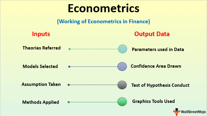
什么是计量经济学?
计量经济学是统计学和数学模型的定量应用,使用数据来发展理论或测试经济学中的现有假设,并根据历史数据预测未来趋势。它对现实世界的数据进行统计试验,然后将结果与被测试的理论进行比较和对比。
根据你是对测试现有理论感兴趣,还是对利用现有数据在这些观察的基础上提出新的假设感兴趣,计量经济学可以细分为两大类:理论和应用。那些经常从事这种实践的人通常被称为计量经济学家。
Matlab代写
MATLAB 是一种用于技术计算的高性能语言。它将计算、可视化和编程集成在一个易于使用的环境中,其中问题和解决方案以熟悉的数学符号表示。典型用途包括:数学和计算算法开发建模、仿真和原型制作数据分析、探索和可视化科学和工程图形应用程序开发,包括图形用户界面构建MATLAB 是一个交互式系统,其基本数据元素是一个不需要维度的数组。这使您可以解决许多技术计算问题,尤其是那些具有矩阵和向量公式的问题,而只需用 C 或 Fortran 等标量非交互式语言编写程序所需的时间的一小部分。MATLAB 名称代表矩阵实验室。MATLAB 最初的编写目的是提供对由 LINPACK 和 EISPACK 项目开发的矩阵软件的轻松访问,这两个项目共同代表了矩阵计算软件的最新技术。MATLAB 经过多年的发展,得到了许多用户的投入。在大学环境中,它是数学、工程和科学入门和高级课程的标准教学工具。在工业领域,MATLAB 是高效研究、开发和分析的首选工具。MATLAB 具有一系列称为工具箱的特定于应用程序的解决方案。对于大多数 MATLAB 用户来说非常重要,工具箱允许您学习和应用专业技术。工具箱是 MATLAB 函数(M 文件)的综合集合,可扩展 MATLAB 环境以解决特定类别的问题。可用工具箱的领域包括信号处理、控制系统、神经网络、模糊逻辑、小波、仿真等。