robotics代写 - 统计代写答疑辅导

分类： robotics代写

robotics代写|寻路算法代写Path Planning Algorithms|Visibility-based Optimal Motion Planning

Posted on 2022年5月12日2022年5月12日 by statistics-lab

如果你也在怎样代写寻路算法Path Planning Algorithms这个学科遇到相关的难题，请随时右上角联系我们的24/7代写客服。

寻路算法被移动机器人、无人驾驶飞行器和自动驾驶汽车所使用，以确定从起点到终点的安全、高效、无碰撞和成本最低的旅行路径。

statistics-lab™ 为您的留学生涯保驾护航在代写寻路算法Path Planning Algorithms方面已经树立了自己的口碑, 保证靠谱, 高质且原创的统计Statistics代写服务。我们的专家在代写寻路算法Path Planning Algorithms代写方面经验极为丰富，各种代写寻路算法Path Planning Algorithms相关的作业也就用不着说。

我们提供的寻路算法Path Planning Algorithms及其相关学科的代写，服务范围广, 其中包括但不限于:

Statistical Inference 统计推断
Statistical Computing 统计计算
Advanced Probability Theory 高等概率论
Advanced Mathematical Statistics 高等数理统计学
(Generalized) Linear Models 广义线性模型
Statistical Machine Learning 统计机器学习
Longitudinal Data Analysis 纵向数据分析
Foundations of Data Science 数据科学基础

robotics代写|寻路算法代写Path Planning Algorithms|Visibility-based Optimal Motion Planning

robotics代写|寻路算法代写Path Planning Algorithms|Observation Of Three-Dimensional Objects

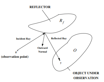
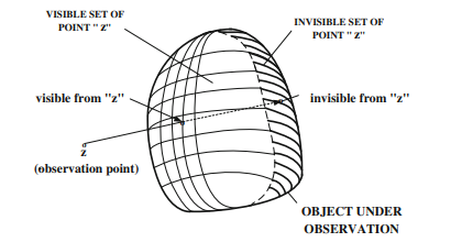
Now, we turn our attention to optimal path planning problems for observing threedimensional objects. As we mentioned in Chap. 2 (Proposition $2.2$ and Remark 2.2) that at least two point-observers are required for total visibility of a solid body in $\mathbb{R}^{3}$. The following lemma gives a sufficient condition for total visibility of a solid body in $\mathbb{R}^{3}$.

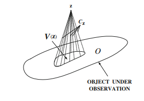
Lemma 4.2 Suppose that the object under observation is a compact simply-connected solid body $\partial \mathcal{O} \subset \mathbb{R}^{3}$ with a smooth boundary $\partial \mathcal{O}$ and no outwardnormal intersection points. Then, total visibility of $\mathcal{O}$ can be attained by a finite set of observation points in the observation platform $\mathcal{P}_{h}$ at a constant finite height $h$ along the outward normal above the body surface $\partial \mathcal{O}$.

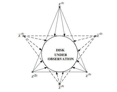
Proof $4.3$ Since $\mathcal{O}$ is a compact simply-connected solid body with a smooth boundary $\partial \mathcal{O}$ and no outward-normal intersection points, then $\mathcal{P}{h}=\left{z \in \mathbb{R}^{3}: z=\right.$ $x+h n(x), x \in \partial \mathcal{O}}$ is well-defined. For any observation point $z \in \mathcal{P}{h}$, there exists a point $x=z-h n(x) \in \partial \mathcal{O}$ such that $x$ is visible from $z$. Moreover, $\mathcal{V}(z)$, the visible set of $z$, is a compact subset of $\partial \mathcal{O}$ containing $x$ with finite measure $\mu_{2}(\partial \mathcal{V}(z))$. Since $\mu_{2}(\mathcal{O})$ is finite, there exists a finite number $N$ of observation points $z^{(i)} \in \mathcal{P}{h}, i=$ $1, \ldots, N$ such that $\partial \mathcal{O} \subseteq \bigcup{i=1}^{N} \mathcal{V}\left(z^{(i)}\right)$ as guaranteed by the Heine-Borel Covering Theorem.

First, we extend Problem 4.1, the shortest path total visibility problem, to the observation of a 3-D object $\mathcal{O}$ by a single mobile-observer.

Problem 4.1A Single Mobile-Observer Shortest Path Problem. Given an observation platform $\mathcal{P}$ enclosing the observed 3-D object $\mathcal{O}$, and two distinct points $z_{o}, z_{f} \in \mathcal{P}$, find the shortest admissible path $\Gamma \mathcal{P}$ starting at $z_{o}$ and ending at $z_{f}$ such that $\bigcup_{z \in \Gamma_{\mathcal{P}}} \mathcal{V}(z)=\partial \mathcal{O}$.

We observe that for $\mathcal{P}=\mathcal{P}{h}$, once a solution to Problem $3.5$ is obtained, any admissible path starting at $z{o}$, passing through all the points in the observation-point set $\mathcal{P}^{(N)}$, and ending at $z_{f}$, is a candidate to the solution of Problem 4.1A.

To illustrate the nature of the solution to Problem 4.1A, we consider a specific example.

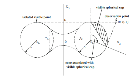
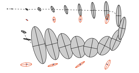
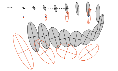
Example $4.5$ Here, the object under observation is a closed spherical ball $\overline{\mathcal{B}}\left(0 ; r_{o}\right)$. The observation platform $\mathcal{P}{h}$ is a sphere $\mathcal{S}\left(0 ; r{o}+h\right)$ with finite observation height $h>0$. From the Principle of Optimality in Dynamic Programming, an optimal path is a concatenation of geodesics starting and ending at distinct specified points $z_{o}, z_{f} \in$ $\mathcal{P}{h}$. Figure $4.13$ shows an optimal path corresponding to $z{o}=\left(0,-\left(r_{o}+h\right), 0\right)$ and $z_{f}=\left(0, r_{o}+h, 0\right)$, with observation height $h$ satisfying $0<\alpha \leq \pi / 4$, where $\alpha=\sin ^{-1}\left(r_{o} /\left(r_{o}+h\right)\right)$ is the half-angle of the observation cone. We observe that the optimal path has length $l_{\min }=3 \pi\left(r_{o}+h\right)$, and has a great-circle loop along the path. For $\alpha>\pi / 4$, there are more than one great-circle loops along the path.

robotics代写|寻路算法代写Path Planning Algorithms|Particular Case

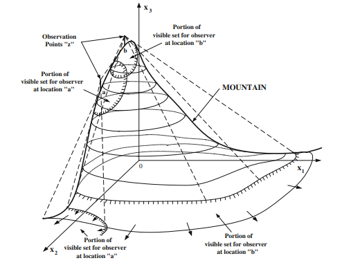
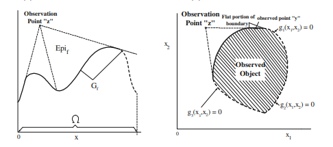
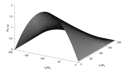
Let $B=\left{e_{1}, \ldots, e_{n}\right}$ be a specified orthonormal bases for the $n$-dimensional real Euclidean space $\mathbb{R}^{n}$, where $e_{i}$ corresponds to the $i$ th unit basis vector. The representation of a point $x \in \mathbb{R}^{n}$ with respect to $B$ is specified by the column vector $\left[x_{1}, \ldots, x_{n}\right]^{T}$. The usual Euclidean norm of $x$ is denoted by $|x|$. Let $f=f(x)$ be a specified real-valued $C_{2}$-function defined on $\Omega$, a specified simply connected, compact subset of $\mathbb{R}^{2}$ with a smooth boundary $\partial \Omega$. As in Chap. 2 , the graph and vation is the spatial terrain surface described by $G_{f}$ in the world space $\mathcal{W}=\mathbb{R}^{3}$. The observation platform $\mathcal{P}$ on which the observers are attached corresponds to the elevated surface of $G_{f}$ given by $G_{f_{h_{v}}}$, where $f_{h_{v}} \stackrel{\text { def }}{=} f+h_{v}$ with $h_{v}$ being a specified positive number. This implies that for any $x \in \Omega$, the observers are at fixed vertical-height $h_{v}$ above the surface $G_{f}$.

From the extension of Proposition $3.1$ to the case where $\operatorname{dim}(\Omega)=2$, there exists a critical vertical-height $h_{v c}(x)$ for each $x \in \Omega$ such that total visibility is attainable. Consider the nontrivial case where $h_{v}<h_{v c}(x)$ for all $x \in \Omega$ so that the mobile observer must move to achieve total visibility. Let $I_{l f}=\left[0, t_{f}\right]$ denote the observation time interval, where $t_{f}$ may be a finite fixed or variable terminal time. For simplicity, the mobile observer is represented by a point mass $M$. Its position in the world space $\mathcal{W}=\mathbb{R}^{3}$ at any time $t$ is specified by $p(t)$ whose representation with respect to a given orthonormal basis $B$ is denoted by $\left[x_{1}(t), x_{2}(t), x_{3}(t)\right]^{T}$, where $x_{3}(t)$ corresponds to the observer position along the $x_{3}$-axis at time $t$. The motion of

the mobile observer can be described by Newton’s law:
$$
\begin{gathered}
M \ddot{x}(t)+\nu_{x} \dot{x}(t)=u(t) \
M \ddot{x}{3}(t)+\nu{3}\left(x(t), \dot{x}(t), x_{3}(t), \dot{x}{3}(t)\right)=\xi(t)-M g, \end{gathered} $$ where $x(t)=\left[x{1}(t), x_{2}(t)\right]^{T} ;(u, \xi)$ is the external force with $u=\left[u_{1}, u_{2}\right]^{T}$ being the control; $-M g$ is the gravitational force in the downward direction along the $x_{3}$-axis. $\nu_{x}$ is a given nonnegative friction coefficient; $\nu_{3}$ is a specified real-valued function of its arguments describing the $x_{3}$-component of the friction force. The variables with single and double overdots denote respectively their first and second derivatives with respect to time $t$. Assuming that the mobile observer is constrained to move on $G_{f}$ at all times without slipping, the mobile observer motion satisfies a holonomic constraint:
$$
x_{3}(t)=f(x(t)) \text { for all } t \in I_{l_{f}},
$$
and a state variable (position) constraint:
$$
x(t) \in \Omega \text { for all } t \in I_{I_{f}} .
$$
Since $f$ is a $C_{2}$-function on $\Omega$, we may differentiate (5.3) twice with respect to $t$ to obtain
$$
\begin{aligned}
&\dot{x}{3}(t)=\nabla{x} f(x(t))^{T} \dot{x}(t) \
&\ddot{x}{3}(t)=\nabla{x} f(x(t))^{T} \ddot{x}(t)+\dot{x}(t)^{T} H_{f}(x(t)) \dot{x}(t),
\end{aligned}
$$
where $\nabla_{x}$ denotes the gradient operator with respect to $x$, and $H_{f}(x(t))$ the Hessian matrix of $f$ with respect to $x$ evaluated at $x(t)$. Substituting (5.5) into (5.2) gives the required vertical component $\xi(t)$ of the external force for keeping the mobile observer on the surface $G_{f}$ at all times:
$$
\begin{aligned}
\xi(t)=& M\left(\nabla_{x} f(x(t))^{T} \ddot{x}(t)+\dot{x}(t)^{T} H_{f}(x(t)) \dot{x}(t)\right) \
&\left.+\nu_{3}\left(x(t), \dot{x}(t), x_{3}(t), \nabla_{x} f(x(t))^{T} \dot{x}(t)\right) / M+g\right) .
\end{aligned}
$$
Assuming that the mobile observer lies on $G_{f}$ at the starting time $t=0$, then
$$
x_{3}(0)=f(x(0)), \quad \dot{x}{3}(0)=\nabla{x} f(x(0))^{T} \dot{x}(0) .
$$
In the foregoing dynamic model of the mobile observer, we have assumed that the $x$-component of the friction force depend only on $\dot{x}$. In general, they may depend on both $(x, \dot{x})$ and $\left(x_{3}, \dot{x}_{3}\right)$. Also, to simplify the subsequent development, we have not considered the surface contact forces in the foregoing model.

robotics代写|寻路算法代写Path Planning Algorithms|Statement of Problems

Now, a few physically meaningful visibility-based optimal motion planning problems can be stated as follows:

Problem 5.1 Minimum-Time Total Visibility Problem. Let $\mathcal{U}{\mathrm{ad}}=\bigcup{t f \geq 0} \mathcal{U}{\mathrm{ad}}\left(I{t f}\right)$ be the set of all admissible controls. Given $s_{x}(0)=(x(0), \dot{x}(0))$ or the initial state of the mobile observer with initial position $p(0)=(x(0), f(x(0))) \in G_{f}$ and initial velocity $v(0)=\left(\dot{x}(0), \nabla_{x} f(x(0))^{T} \dot{x}(0)\right)$, find the smallest time $t_{f}^{} \geq 0$ and an admissible control $u^{}=u^{}(t)$ defined on $I_{l_{f}^{}}$ such that its corresponding motion or time-dependent path $\Gamma_{i_{f}^{}}=\left{\left(x_{u^{}}(t), f\left(x_{u^{}}(t)\right)\right) \in \mathbb{R}^{3}: t \in I_{t_{f}^{}}\right}$ on the surface $G_{f}$ satisfies the total visibility condition at $t_{f}^{}$ : $$ \bigcup_{t \in I_{t_{f}^{}}} \mathcal{V}\left(\left(x_{u^{}}(t), f_{h_{v}}\left(x_{u^{}}(t)\right)\right)=G_{f}\right.
$$
or alternatively,
$$
\mu_{2}\left{\bigcup_{t \in I_{t}^{}} \Pi_{\Omega} \mathcal{V}\left(\left(x_{u^{}}(t), f_{h_{v}}\left(x_{u^{}}(t)\right)\right)\right}=\mu_{2}{\Omega},\right. $$ where $\mu_{2}{\sigma}$ denotes the Lebesgue measure of the set $\sigma \subset \mathbb{R}^{2}$. In the foregoing problem statement, condition (5.10) only involves the position $x_{u^{}}(t)$, not the velocity $\dot{x}{u^{}}(t)$. In certain physical situations, it is required to move the mobile observer from one rest position to another, i.e. $\dot{x}{u^{}}(0)=0$ and $\dot{x}{u^{}}\left(t{f}^{}\right)=0$. Also, in planetary surface exploration, it is important to avoid paths with steep slopes. This suggests the inclusion of the following gradient constraint in Problem 5.1:
$$
\left|\nabla_{x} f\left(x_{u^{}}(t)\right)\right| \leq f_{\max }^{\prime} \text { for all } t \in I_{t_{f}^{}},
$$
where $f_{\max }^{\prime}$ is a specified positive number. Now, if the set $\Omega^{\text {def }}=\left{x \in \Omega: | \nabla_{x} f\left(x_{u^{*}}(t)\right)\right.$ $\left.| \leq f_{\max }^{\prime}\right}$ is a simply connected compact subset of $\mathbb{R}^{2}$, then we may replace $\Omega$ in Problem $5.1$ by $\Omega^{\prime}$ to take care of constraint (5.12).

Problem 5.2 Maximum Visibility Problem with Fixed Observation TimeInterval. Given a finite observation time interval $I_{I_{f}}$ and $s_{x}(0)=(x(0), \dot{x}(0))$, or the initial state of the mobile observer with initial position $p(0)=(x(0), f(x(0))) \in G_{f}$ and initial velocity $v(0)=\left(\dot{x}(0), \nabla_{x} f(x(0))^{T} \dot{x}(0)\right)$ at $t=0$, find an admissible control $u^{}=u^{}(t)$ and its corresponding motion or time-dependent path $\Gamma_{t_{f}}^{}=\left{\left(x_{u t^{}}(t), f\left(x_{u}^{*}(t)\right)\right) \in \mathbb{R}^{3}: t \in I_{t f}\right} \subset G_{f}$ such that the visibility functional given by

$$
J_{1}(u)=\int_{0}^{t f} \mu_{2}\left{\Pi_{\Omega} \mathcal{V}\left(\left(x_{u}(t), f_{h_{v}}\left(x_{u}(t)\right)\right)\right)\right} d t
$$
is defined, and satisfies $J_{1}\left(u^{}\right) \geq J_{1}(u)$ for all $u\left({ }^{}\right) \in \mathcal{U}{\mathrm{ad}}\left(I{t_{f}}\right)$.
Another meaningful visibility functional is given by
$$
J_{2}(u)=\mu_{2}\left{\bigcup_{t \in I_{t}} \Pi_{\Omega} \mathcal{V}\left(\left(x_{u}(t), f_{h_{v}}\left(x_{u t}(t)\right)\right)\right)\right} .
$$
The foregoing problem with $J_{1}$ replaced by $J_{2}$ corresponds to selecting an admissible control $u^{}(\cdot)$ such that the area of the union of the projected visibility sets on $\Omega$ for all the points along the corresponding time-dependent path $\Gamma_{t_{f}}^{}$ is maximized.

寻路算法代写

robotics代写|寻路算法代写Path Planning Algorithms|Observation Of Three-Dimensional Objects

现在，我们将注意力转向观察三维物体的最优路径规划问题。正如我们在第一章中提到的。2（命题2.2和备注 2.2) 至少需要两个点观察者才能在R3. 以下引理给出了实体在R3.

引理 4.2 假设被观察的物体是一个紧致的单连通固体∂这⊂R3具有平滑的边界∂这并且没有外法相交点。然后，总能见度这可以通过观察平台中的一组有限的观察点来获得磷H在恒定的有限高度H沿着体表上方的外法线∂这.

证明4.3自从这是具有光滑边界的紧致简连实体∂这并且没有向外法线交点，那么\mathcal{P}{h}=\left{z \in \mathbb{R}^{3}: z=\right.$ $x+h n(x), x \in \partial \mathcal{O}}\mathcal{P}{h}=\left{z \in \mathbb{R}^{3}: z=\right.$ $x+h n(x), x \in \partial \mathcal{O}}是明确的。对于任何观察点和∈磷H, 存在一个点X=和−Hn(X)∈∂这这样X从可见和. 而且，在(和)，可见集和, 是的紧子集∂这包含X有限度μ2(∂在(和)). 自从μ2(这)是有限的，存在一个有限的数ñ观察点和(一世)∈磷H,一世= 1,…,ñ这样∂这⊆⋃一世=1ñ在(和(一世))由 Heine-Borel 覆盖定理保证。

首先，我们将问题 4.1（最短路径总能见度问题）扩展到对 3-D 对象的观察这由单个移动观察者。

问题 4.1 单个移动观察者最短路径问题。给定一个观察平台磷封闭观察到的 3-D 对象这, 和两个不同的点和这,和F∈磷, 找到最短允许路径Γ磷开始于和这并结束于和F这样⋃和∈Γ磷在(和)=∂这.

我们观察到对于磷=磷H, 一旦解决问题3.5获得，任何可接受的路径开始于和这，通过观察点集中的所有点磷(ñ), 并结束于和F, 是问题 4.1A 解决方案的候选项。

为了说明问题 4.1A 解决方案的性质，我们考虑一个具体的例子。

例子4.5这里，被观察的物体是一个封闭的球体乙¯(0;r这). 观景台磷H是一个球体小号(0;r这+H)观察高度有限H>0. 根据动态规划中的最优性原理，最优路径是在不同指定点开始和结束的测地线的串联和这,和F∈ 磷H. 数字4.13显示对应于的最佳路径和这=(0,−(r这+H),0)和和F=(0,r这+H,0), 有观察高度H令人满意的0<一种≤圆周率/4，在哪里一种=罪−1⁡(r这/(r这+H))是观察锥的半角。我们观察到最优路径有长度l分钟=3圆周率(r这+H)，并且沿着路径有一个大圆环。为了一种>圆周率/4，沿路径有不止一个大圆环。

robotics代写|寻路算法代写Path Planning Algorithms|Particular Case

让B=\left{e_{1}, \ldots, e_{n}\right}B=\left{e_{1}, \ldots, e_{n}\right}是指定的正交基n维实欧几里得空间Rn，在哪里和一世对应于一世th 单位基向量。一个点的表示X∈Rn关于乙由列向量指定[X1,…,Xn]吨. 通常的欧几里得范数X表示为|X|. 让F=F(X)是一个指定的实值C2-函数定义在Ω，一个指定的简单连接，紧凑的子集R2具有平滑的边界∂Ω. 就像在第一章中一样。2 , graph 和 vation 是描述的空间地形表面GF在世界空间在=R3. 观景台磷观察者所在的位置对应于高架表面GF由GFH在，在哪里FH在= 定义 F+H在和H在是一个指定的正数。这意味着对于任何X∈Ω，观察者处于固定的垂直高度H在表面之上GF.

从命题的延伸3.1到的情况暗淡⁡(Ω)=2, 存在临界垂直高度H在C(X)对于每个X∈Ω这样才能获得完全的可见性。考虑不平凡的情况，其中H在<H在C(X)对全部X∈Ω因此移动观察者必须移动以实现完全可见性。让一世lF=[0,吨F]表示观察时间间隔，其中吨F可以是有限的固定或可变终止时间。为简单起见，移动观察者由点质量表示米. 它在世界空间中的位置在=R3随时吨由指定p(吨)其关于给定正交基的表示乙表示为[X1(吨),X2(吨),X3(吨)]吨，在哪里X3(吨)对应于沿观察者的位置X3-轴在时间吨. 的动议

移动观察者可以用牛顿定律来描述：
米X¨(吨)+νXX˙(吨)=在(吨) 米X¨3(吨)+ν3(X(吨),X˙(吨),X3(吨),X˙3(吨))=X(吨)−米G,在哪里X(吨)=[X1(吨),X2(吨)]吨;(在,X)是外力与在=[在1,在2]吨作为控制；−米G是沿向下方向的重力X3-轴。νX是给定的非负摩擦系数；ν3是其参数的指定实值函数，描述X3- 摩擦力的分量。带有单点和双点的变量分别表示它们关于时间的一阶和二阶导数吨. 假设移动观察者被限制继续前进GF在任何时候都没有滑动，移动的观察者运动满足一个完整的约束：
X3(吨)=F(X(吨)) 对全部吨∈一世lF,
和一个状态变量（位置）约束：
X(吨)∈Ω 对全部吨∈一世一世F.
自从F是一个C2- 功能开启Ω, 我们可以将 (5.3) 微分两次吨获得
X˙3(吨)=∇XF(X(吨))吨X˙(吨) X¨3(吨)=∇XF(X(吨))吨X¨(吨)+X˙(吨)吨HF(X(吨))X˙(吨),
在哪里∇X表示关于的梯度算子X，和HF(X(吨))的 Hessian 矩阵F关于X评价为X(吨). 将 (5.5) 代入 (5.2) 得到所需的垂直分量X(吨)使移动观察者保持在表面上的外力GF每时每刻：
X(吨)=米(∇XF(X(吨))吨X¨(吨)+X˙(吨)吨HF(X(吨))X˙(吨)) +ν3(X(吨),X˙(吨),X3(吨),∇XF(X(吨))吨X˙(吨))/米+G).
假设移动观察者位于GF在开始时间吨=0，然后
X3(0)=F(X(0)),X˙3(0)=∇XF(X(0))吨X˙(0).
在上述移动观察者的动态模型中，我们假设X- 摩擦力的分量仅取决于X˙. 一般来说，它们可能取决于两者(X,X˙)和(X3,X˙3). 另外，为了简化后续开发，我们没有考虑上述模型中的表面接触力。

robotics代写|寻路算法代写Path Planning Algorithms|Statement of Problems

现在，一些物理上有意义的基于可见性的最优运动规划问题可以表述如下：

问题 5.1 最小时间总能见度问题。让在一种d=⋃吨F≥0在一种d(一世吨F)是所有允许控制的集合。给定sX(0)=(X(0),X˙(0))或具有初始位置的移动观察者的初始状态p(0)=(X(0),F(X(0)))∈GF和初速度在(0)=(X˙(0),∇XF(X(0))吨X˙(0)), 找到最小的时间吨F≥0和一个可接受的控制在=在(吨)定义于一世lF使得其相应的运动或时间相关的路径\Gamma_{i_{f}^{}}=\left{\left(x_{u^{}}(t), f\left(x_{u^{}}(t)\right)\right) \在 \mathbb{R}^{3}: t \in I_{t_{f}^{}}\right}\Gamma_{i_{f}^{}}=\left{\left(x_{u^{}}(t), f\left(x_{u^{}}(t)\right)\right) \在 \mathbb{R}^{3}: t \in I_{t_{f}^{}}\right}在表面上GF满足总能见度条件吨F :⋃吨∈一世吨F在((X在(吨),FH在(X在(吨)))=GF
或者，
\mu_{2}\left{\bigcup_{t \in I_{t}^{}} \Pi_{\Omega} \mathcal{V}\left(\left(x_{u^{}}(t), f_{h_{v}}\left(x_{u^{}}(t)\right)\right)\right}=\mu_{2}{\Omega},\right。\mu_{2}\left{\bigcup_{t \in I_{t}^{}} \Pi_{\Omega} \mathcal{V}\left(\left(x_{u^{}}(t), f_{h_{v}}\left(x_{u^{}}(t)\right)\right)\right}=\mu_{2}{\Omega},\right。在哪里μ2σ表示集合的 Lebesgue 测度σ⊂R2. 在上述问题陈述中，条件（5.10）只涉及位置X在(吨)，而不是速度X˙在(吨). 在某些物理情况下，需要将移动观察者从一个静止位置移动到另一个静止位置，即X˙在(0)=0和X˙在(吨F)=0. 此外，在行星表面探测中，重要的是要避开陡坡的路径。这表明在问题 5.1 中包含以下梯度约束：
|∇XF(X在(吨))|≤F最大限度′ 对全部吨∈一世吨F,
在哪里F最大限度′是一个指定的正数。现在，如果集合\Omega^{\text {def }}=\left{x \in \Omega: | \nabla_{x} f\left(x_{u^{*}}(t)\right)\right.$ $\left.| \leq f_{\max }^{\prime}\right}\Omega^{\text {def }}=\left{x \in \Omega: | \nabla_{x} f\left(x_{u^{*}}(t)\right)\right.$ $\left.| \leq f_{\max }^{\prime}\right}是一个简单连通的紧子集R2，那么我们可以替换Ω在问题5.1经过Ω′照顾约束（5.12）。

问题 5.2 固定观察时间间隔的最大能见度问题。给定一个有限的观察时间间隔一世一世F和sX(0)=(X(0),X˙(0))，或具有初始位置的移动观察者的初始状态p(0)=(X(0),F(X(0)))∈GF和初速度在(0)=(X˙(0),∇XF(X(0))吨X˙(0))在吨=0, 找到一个可接受的控制在=在(吨)及其相应的运动或时间相关路径\Gamma_{t_{f}}^{}=\left{\left(x_{ut^{}}(t), f\left(x_{u}^{*}(t)\right)\right) \in \mathbb{R}^{3}: t \in I_{t f}\right} \subset G_{f}\Gamma_{t_{f}}^{}=\left{\left(x_{ut^{}}(t), f\left(x_{u}^{*}(t)\right)\right) \in \mathbb{R}^{3}: t \in I_{t f}\right} \subset G_{f}使得可见性函数由下式给出J_{1}(u)=\int_{0}^{t f} \mu_{2}\left{\Pi_{\Omega} \mathcal{V}\left(\left(x_{u}(t), f_{h_{v}}\left(x_{u}(t)\right)\right)\right)\right} d tJ_{1}(u)=\int_{0}^{t f} \mu_{2}\left{\Pi_{\Omega} \mathcal{V}\left(\left(x_{u}(t), f_{h_{v}}\left(x_{u}(t)\right)\right)\right)\right} d t
被定义，并且满足Ĵ1(在)≥Ĵ1(在)对全部在()∈在一种d(一世吨F).
另一个有意义的可见性函数由下式给出
J_{2}(u)=\mu_{2}\left{\bigcup_{t \in I_{t}} \Pi_{\Omega} \mathcal{V}\left(\left(x_{u}(t ), f_{h_{v}}\left(x_{ut}(t)\right)\right)\right)\right} 。J_{2}(u)=\mu_{2}\left{\bigcup_{t \in I_{t}} \Pi_{\Omega} \mathcal{V}\left(\left(x_{u}(t ), f_{h_{v}}\left(x_{ut}(t)\right)\right)\right)\right} 。
上述问题与Ĵ1取而代之Ĵ2对应于选择一个可接受的控制在(⋅)使得投影能见度的并集区域设置为Ω对于沿相应时间相关路径的所有点Γ吨F被最大化。

robotics代写|寻路算法代写Path Planning Algorithms 请认准statistics-lab™

统计代写请认准statistics-lab™. statistics-lab™为您的留学生涯保驾护航。

金融工程代写

金融工程是使用数学技术来解决金融问题。金融工程使用计算机科学、统计学、经济学和应用数学领域的工具和知识来解决当前的金融问题，以及设计新的和创新的金融产品。

非参数统计代写

非参数统计指的是一种统计方法，其中不假设数据来自于由少数参数决定的规定模型；这种模型的例子包括正态分布模型和线性回归模型。

广义线性模型代考

广义线性模型（GLM）归属统计学领域，是一种应用灵活的线性回归模型。该模型允许因变量的偏差分布有除了正态分布之外的其它分布。

术语广义线性模型（GLM）通常是指给定连续和/或分类预测因素的连续响应变量的常规线性回归模型。它包括多元线性回归，以及方差分析和方差分析（仅含固定效应）。

有限元方法代写

有限元方法（FEM）是一种流行的方法，用于数值解决工程和数学建模中出现的微分方程。典型的问题领域包括结构分析、传热、流体流动、质量运输和电磁势等传统领域。

有限元是一种通用的数值方法，用于解决两个或三个空间变量的偏微分方程（即一些边界值问题）。为了解决一个问题，有限元将一个大系统细分为更小、更简单的部分，称为有限元。这是通过在空间维度上的特定空间离散化来实现的，它是通过构建对象的网格来实现的：用于求解的数值域，它有有限数量的点。边界值问题的有限元方法表述最终导致一个代数方程组。该方法在域上对未知函数进行逼近。[1] 然后将模拟这些有限元的简单方程组合成一个更大的方程系统，以模拟整个问题。然后，有限元通过变化微积分使相关的误差函数最小化来逼近一个解决方案。

tatistics-lab作为专业的留学生服务机构，多年来已为美国、英国、加拿大、澳洲等留学热门地的学生提供专业的学术服务，包括但不限于Essay代写，Assignment代写，Dissertation代写，Report代写，小组作业代写，Proposal代写，Paper代写，Presentation代写，计算机作业代写，论文修改和润色，网课代做，exam代考等等。写作范围涵盖高中，本科，研究生等海外留学全阶段，辐射金融，经济学，会计学，审计学，管理学等全球99%专业科目。写作团队既有专业英语母语作者，也有海外名校硕博留学生，每位写作老师都拥有过硬的语言能力，专业的学科背景和学术写作经验。我们承诺100%原创，100%专业，100%准时，100%满意。

随机分析代写

随机微积分是数学的一个分支，对随机过程进行操作。它允许为随机过程的积分定义一个关于随机过程的一致的积分理论。这个领域是由日本数学家伊藤清在第二次世界大战期间创建并开始的。

时间序列分析代写

随机过程，是依赖于参数的一组随机变量的全体，参数通常是时间。随机变量是随机现象的数量表现，其时间序列是一组按照时间发生先后顺序进行排列的数据点序列。通常一组时间序列的时间间隔为一恒定值（如1秒，5分钟，12小时，7天，1年），因此时间序列可以作为离散时间数据进行分析处理。研究时间序列数据的意义在于现实中，往往需要研究某个事物其随时间发展变化的规律。这就需要通过研究该事物过去发展的历史记录，以得到其自身发展的规律。

回归分析代写

多元回归分析渐进（Multiple Regression Analysis Asymptotics）属于计量经济学领域，主要是一种数学上的统计分析方法，可以分析复杂情况下各影响因素的数学关系，在自然科学、社会和经济学等多个领域内应用广泛。

MATLAB代写

MATLAB 是一种用于技术计算的高性能语言。它将计算、可视化和编程集成在一个易于使用的环境中，其中问题和解决方案以熟悉的数学符号表示。典型用途包括：数学和计算算法开发建模、仿真和原型制作数据分析、探索和可视化科学和工程图形应用程序开发，包括图形用户界面构建MATLAB 是一个交互式系统，其基本数据元素是一个不需要维度的数组。这使您可以解决许多技术计算问题，尤其是那些具有矩阵和向量公式的问题，而只需用 C 或 Fortran 等标量非交互式语言编写程序所需的时间的一小部分。MATLAB 名称代表矩阵实验室。MATLAB 最初的编写目的是提供对由 LINPACK 和 EISPACK 项目开发的矩阵软件的轻松访问，这两个项目共同代表了矩阵计算软件的最新技术。MATLAB 经过多年的发展，得到了许多用户的投入。在大学环境中，它是数学、工程和科学入门和高级课程的标准教学工具。在工业领域，MATLAB 是高效研究、开发和分析的首选工具。MATLAB 具有一系列称为工具箱的特定于应用程序的解决方案。对于大多数 MATLAB 用户来说非常重要，工具箱允许您学习和应用专业技术。工具箱是 MATLAB 函数（M 文件）的综合集合，可扩展 MATLAB 环境以解决特定类别的问题。可用工具箱的领域包括信号处理、控制系统、神经网络、模糊逻辑、小波、仿真等。

R语言代写	问卷设计与分析代写
PYTHON代写	回归分析与线性模型代写
MATLAB代写	方差分析与试验设计代写
STATA代写	机器学习/统计学习代写
SPSS代写	计量经济学代写
EVIEWS代写	时间序列分析代写
EXCEL代写	深度学习代写
SQL代写	各种数据建模与可视化代写

robotics代写|寻路算法代写Path Planning Algorithms|Visibility-Based Optimal Path Planning

Posted on 2022年5月12日2022年5月12日 by statistics-lab

如果你也在怎样代写寻路算法Path Planning Algorithms这个学科遇到相关的难题，请随时右上角联系我们的24/7代写客服。

寻路算法被移动机器人、无人驾驶飞行器和自动驾驶汽车所使用，以确定从起点到终点的安全、高效、无碰撞和成本最低的旅行路径。

我们提供的寻路算法Path Planning Algorithms及其相关学科的代写，服务范围广, 其中包括但不限于:

Statistical Inference 统计推断
Statistical Computing 统计计算
Advanced Probability Theory 高等概率论
Advanced Mathematical Statistics 高等数理统计学
(Generalized) Linear Models 广义线性模型
Statistical Machine Learning 统计机器学习
Longitudinal Data Analysis 纵向数据分析
Foundations of Data Science 数据科学基础

robotics代写|寻路算法代写Path Planning Algorithms|Visibility-Based Optimal Path Planning

robotics代写|寻路算法代写Path Planning Algorithms|Existence of Solutions

First, we consider Problem 4.1. The following result ensures that the set of all admissible paths $\Gamma$ satisfying condition (1) is nonempty.

Proposition 4.1 Under the conditions of Theorem 3.3, there exists an admissible path $\Gamma \in \Omega$ that satisfies condition (4.2).

Proof 4.I From Theorem $3.3$, there exists a finite point set $P^{(N)}=\left{x^{(k)}, k=\right.$ $1, \ldots, N} \subset \Omega$ that satisfies the total visibility constraint (1). If the specified end points $x_{o}$ and $x_{f} \in P^{(N)}$, then under the assumption that $\Omega$ is simply connected, it is always possible to construct a path $\Gamma$ in $\Omega$ corresponding to a Jordan arc passing through all the points in $P^{(N)}$. In particular, if the line segment joining any pair of points in $P^{(N)}$ lies in $\Omega$, then a Jordan arc composed of straightline segments joining the successive points in $P^{(N)}$ can always be constructed. A trivial case is where $\Omega$ is a compact convex subset of $\mathbb{R}^{2}$. If $x_{o}$ and/or $x_{f} \notin P^{(N)}$, we augment $P^{(N)}$ by these points, and proceed with the construction of a Jordan arc. Finally, from the constructed $\Gamma$, the corresponding path $\Gamma_{\mathcal{P}}$ in $\mathcal{P}$ can be determined from ${(x, g(x)): x \in \Gamma} .$

Remark 4.3 Proposition $4.1$ implies the existence of a Jordan arc passing through a finite set of observation points $\left(x^{(k)}, f_{h_{v}}\left(x^{(k)}\right)\right) \in G_{f_{b_{E}}}$ such that $G_{f}$ is totally visible. In general, the set of observation points for total visibility is not unique. Moreover, the cardinality of this set depends on $f$.

Remark 4.4 Suppose that the line segment $L$ joining the points $x_{o}$ and $x_{f}$ lies in $\Omega$, and $\bigcup_{x \in L} \mathcal{V}\left(\left(x, f_{h_{E}}(x)\right)\right)=G_{f}$, then $L$ is an optimal path. If $\bigcup_{x \in L} \mathcal{V}\left(\left(x, f_{h_{v}}(x)\right)\right) \subset$ $G_{f}$, then for a certain class of $G_{f}$, the optimal path $\Gamma^{*}$ is close to $L$ in the sense of arc length. Minimal excursions from $L$ can be introduced so that the invisible part $G_{f}-\bigcup_{x \in L} \mathcal{V}\left(\left(x, f_{h_{v}}(x)\right)\right)$ becomes visible.

For Problem 4.1″, we first construct the set $\tilde{\Omega} \stackrel{\text { def }}{=}\left{x \in \Omega:|\nabla f(x)| \leq f_{\max }^{\prime}\right}$, and then find the shortest admissible path $\Gamma^{} \subset \bar{\Omega}$ such that $\bigcup_{x \in \Gamma^{}} \mathcal{V}\left(\left(x, f_{h_{v}}(x)\right)\right)=$ $G_{f}$. In general, it is possible that $\bar{\Omega}$ consists of disjoint subsets of $\Omega$, and there may not exist admissible paths in $\bar{\Omega}$ (e.g. $x_{o}$ and $x_{f}$ lie in two disjoint subsets of $\Omega$ separated by a strip on which $|\nabla f(x)|>f_{\max }^{\prime}$ for all points $x$ on this strip). Consequently, Problem 4.1″ has no solution. Note also that the line segment $L$ joining $x_{o}$ and $x_{f}$ may not lie in $\bar{\Omega}$.

Since $f$ is a $C_{1}$-function, the set $\bar{\Omega}$ is compact. Assuming the existence of an admissible path in $\bar{\Omega}$, the observations given in Remarks $4.3$ and $4.4$ are also applicable to this case.

robotics代写|寻路算法代写Path Planning Algorithms|Optimality Conditions

Here, we develop optimality conditions for Problem $4.1$ under the assumption that a solution exists. From Theorem $3.3$, there exists a finite point set $P^{(N)}=\left{x^{(k)}, k=\right.$ $1, \ldots, N} \subset \Omega$ with $x^{(1)}=x_{o}$ and $x^{(N)}=x_{f}$ such that
$$
\bigcup_{k=1}^{N} \mathcal{V}\left(\left(x^{(k)}, f_{h_{v}}\left(x^{(k)}\right)\right)\right)=G_{f}
$$
is satisfied. Let $P$ denote the set of all such $P^{(N)}$ ‘s with $2 \leq N<\infty$. The cardinality of $P$ is generally infinite. Now, for a given $P^{(N)} \subset P$, let $\tilde{\mathcal{A}}{P(N)}$ denote the set of all admissible paths $\Gamma$ formed by line segments joining distinct pairs of points in $P^{(N)}$. The cardinality of $\overline{\mathcal{A}}{P(N)}$ is $\leq(N-2)$ !. Thus, Problem $4.1$ reduces to finding a finite point set $P^{(N)} \subset P$ and an admissible path $\Gamma \in \tilde{\mathcal{A}}{P(N)}$ such that the arc length $$ \Lambda(\Gamma)=\sum{k=1}^{N-1}\left|x^{(k+1)}-x^{(k)}\right|
$$
is minimized. For convenience, the points $x^{(k)}, k=2, \ldots, N-1$ are indexed consecutively along the path $\Gamma$ initiating from $x_{o}$ and moving towards the end point $x_{f}$.
The following simple necessary condition for optimality can be deduced readily from the definition of arc length:

Proposition $4.2$ Let $\Gamma^{}$ be an optimal admissible path for Problem 4.1, and $P^{\left(N^{}\right)}=$ $\left{x_{}^{(k)} \in \Gamma^{}, k=1, \ldots, N^{}\right}$ be a finite point set satisfying (4.16). Then, for any perturbed admissible path $\Gamma \in \overline{\mathcal{A}}{\bar{P}^{\left(N^{}\right)}}$ with finite point set $\left{x{}^{(1)}, \ldots, x_{}^{(k-1)}, x_{}^{(k)}+\right.$ $\left.\delta x, x_{}^{(k+1)}, \ldots, x_{}^{\left(N^{}\right)}\right}$ in which the point perturbation $\delta x$ about $x_{}^{(k)}$ satisfies $x_{}^{(k)}+$ $\delta x \in \Omega$, and condition (4.16) holds, the following inequality:

$$
\begin{aligned}
&\left|x_{}^{(k)}+\delta x-x_{}^{(k-1)}\right|+\left|x_{}^{(k+1)}-x_{}^{(k)}-\delta x\right| \geq\left|x_{}^{(k+1)}-x_{}^{(k)}\right| \
&\quad+\left|x_{}^{(k)}-x_{}^{(k-1)}\right|, \quad k=2, \ldots, N^{}-1, \end{aligned} $$ must be satisfied. For Problem 4.2, a necessary condition for optimality can be derived by considering local path perturbations. Let $I=[0,1]$. First, we parameterize an admissible path $\Gamma$ by the scalar parameter $\lambda \in I$, i.e. $$ \Gamma=\left{\left(x_{1}, x_{2}\right) \in \Omega: x_{1}=q_{1}(\lambda), x_{2}=q_{2}(\lambda), \lambda \in I\right} $$ where $q_{1}$ and $q_{2}$ are real-valued $C_{1}$-functions on $I$ satisfying $$ \left(q_{1}(0), q_{2}(0)\right)=\left(x_{o 1}, x_{o 2}\right) \text { and }\left(q_{1}(1), q_{2}(1)\right)=\left(x_{f 1}, x_{f 2}\right) $$ Let $\Gamma^{}$ and $\Gamma$ denote an optimal path and an admissible perturbed path specified by $q^{}(\lambda)=\left(q_{1}^{}(\lambda), q_{2}^{}(\lambda)\right)$ and $q^{}(\lambda)+\eta(\lambda)=\left(q_{1}^{}(\lambda)+\eta_{1}(\lambda), q_{2}^{}(\lambda)+\eta_{2}(\lambda)\right), \quad \lambda \in I$,
respectively, where $\eta=\left(\eta_{1}, \eta_{2}\right) \in \Sigma_{\Gamma^{}}$, the set of all admissible path perturbations about $\Gamma^{}$ defined by $\Sigma_{\Gamma^{}}=\left{\eta \in C_{1}\left(I ; \mathbb{R}^{2}\right): \eta(0)=(0,0), \eta(1)=(0,0) ; q^{}(\lambda)+\right.$ $\eta(\lambda) \in \Omega$ for all $\lambda \in I}$, with $C_{1}\left(I ; \mathbb{R}^{2}\right)$ being the normed linear space of all continuous functions defined on $I$ with their values in $\mathbb{R}^{2}$ and having continuous first derivatives on $I$, and normed by: $|\eta|_{m}=\sum_{i=1,2}\left(\max {\lambda \in I}\left|\eta{i}(\lambda)\right|+\max {\lambda \in I}\left|\eta{i}^{\prime}(\lambda)\right|\right)$, where $(\cdot)^{\prime}$ denotes differentiation with respect to $\lambda$.

robotics代写|寻路算法代写Path Planning Algorithms|Numerical Algorithms

To facilitate the development of numerical algorithms for the optimal path planning problems, a mesh on $\Omega$ using standard methods such as Delaunay triangulation is established. Then $G_{f}$ is approximated by a polyhedral surface $\hat{G}{f}$, in particular, a surface formed by triangular patches. In practical situations, the function $f=f(x)$ is usually given in the form of numerical data. An approximation of $G{f}$ can be obtained by interpolation of the given numerical data. Here, algorithms are developed for the approximate Problems $4.1$ and $4.2$ that make use of the numerical data directly.
For the Shortest Path Problem 4.1, consider the simplest case where the line segment $L$ joining the end points $x_{o}$ and $x_{f}$ lies in $\Omega$. Remark $4.4$ suggests that a possible approach to obtaining a solution to the approximate Problem $4.1$ is to seek first a finite number of points along $L$ having maximal visibility, and then introduce additional points close to $L$ to achieve total visibility. Finally, a Jordan-arc with minimal length passing through all the observation points is constructed.

Suppose that on $\Omega$, a mesh consisting of points $x^{(k)}, k=1, \ldots, M$ along with the approximate surface $\hat{G}{f}$ formed by triangular patches have been established. For convenience, let $x^{(1)}=x{o}$ and $x^{(M)}=x_{f}$. Let $\hat{\mathcal{G}}$ denote the set of all Jordan arcs connecting $x^{(1)}$ and $x^{(M)}$ formed by line segments corresponding to the edges of the triangles. The basic steps in our algorithm for determining an optimal path for the approximate Problem $4.1$ without assuming that the line segment $L$ joining $x_{o}$ and $x_{f}$ lies in $\Omega$ are as follows:

Step 3 Determine $\hat{\mathcal{G}}^{}=\left{\Gamma_{j}^{}, j=1, \ldots, K\right}$, the set of all Jordan arcs in $\hat{\mathcal{G}}$ having the shortest path length.
Step 4 Select a path in $\hat{\mathcal{G}}^{}$, say $\Gamma_{i}^{}$.
Step 5 Compute the visible set $\mathcal{V}\left(\left(x^{(k)}, f_{h_{v}}\left(x^{(k)}\right)\right)\right)$ corresponding to each point $x^{(k)}$ along the path $\Gamma_{i}^{}$ and its projection $\Pi_{\Omega} \mathcal{V}\left(\left(x^{(k)}, f_{h_{v}}\left(x^{(k)}\right)\right)\right)$. Step 6 Determine whether there exists a combination of points $x^{(k)}$ along $\Gamma_{i}^{}$ such that the union of their visible sets $\mathcal{V}\left(\left(x^{(k)}, f_{h_{v}}\left(x^{(k)}\right)\right)\right)$ is equal to $G_{f}$.
If YES, then $\Gamma_{i}^{}$ is an optimal path for the approximate Problem 4.1, STOP; if NO, select a neighboring path of $\Gamma_{i}^{}$ in the sense of arc length, and GO TO Step $5 .$

Remark $4.5$ In Steps 2 and 3, instead of considering triangles in $\Omega$, we may consider triangular patches associated with the polyhedral approximation of the surface $G_{f}$. Efficient algorithms for computing the shortest arc length such as those due to Sharir and Shorr [3], O’Rourke et al. [4], and Lawler [5] may be used.

Remark $4.6$ Step 5 involves the computation of visible sets $\mathcal{V}\left(\left(x^{(k)}, f_{h_{x}}\left(x^{(k)}\right)\right)\right)$ associated with points $x^{(k)}$ along the path $\Gamma_{i}^{*}$, an NP-hard problem in computational geometry. This task can be accomplished using a suitable algorithm developed recently by Balmes and Wang [1]. The complexity of that algorithm is $O\left(n p^{2}\right)$, where $n$ and $p$ are the number of observation points and the number of triangular patches respectively. This algorithm can be easily modified to take into account the limited aperture of cameras or sensors.

寻路算法代写

robotics代写|寻路算法代写Path Planning Algorithms|Existence of Solutions

首先，我们考虑问题 4.1。以下结果确保了所有允许路径的集合Γ满足条件（1）是非空的。

命题 4.1 在定理 3.3 的条件下，存在一条允许路径Γ∈Ω满足条件（4.2）。

证明 4.I 来自定理3.3, 存在一个有限点集P^{(N)}=\left{x^{(k)}, k=\right.$ $1, \ldots, N} \subset \OmegaP^{(N)}=\left{x^{(k)}, k=\right.$ $1, \ldots, N} \subset \Omega满足总可见性约束 (1)。如果指定的端点X这和XF∈磷(ñ), 那么假设Ω是简单的连接，总是可以构造一个路径Γ在Ω对应于一条穿过所有点的 Jordan 弧磷(ñ). 特别是，如果连接任意一对点的线段磷(ñ)在于Ω，然后由连接连续点的直线段组成的若尔当弧磷(ñ)总是可以构建的。一个微不足道的情况是Ω是一个紧凸子集R2. 如果X这和/或XF∉磷(ñ)，我们增加磷(ñ)通过这些点，继续构建约旦弧。最后，从构建的Γ, 对应路径Γ磷在磷可以从(X,G(X)):X∈Γ.

备注 4.3 命题4.1意味着存在一条通过有限观测点集的若尔当弧(X(ķ),FH在(X(ķ)))∈GFb和这样GF是完全可见的。一般来说，总能见度的观察点集合不是唯一的。此外，这个集合的基数取决于F.

备注 4.4 假设线段大号加入点X这和XF在于Ω，和⋃X∈大号在((X,FH和(X)))=GF，然后大号是一条最优路径。如果⋃X∈大号在((X,FH在(X)))⊂ GF, 那么对于某一类GF, 最优路径Γ∗接近大号在弧长的意义上。最少的游览大号可以引入使不可见的部分GF−⋃X∈大号在((X,FH在(X)))变得可见。

对于问题 4.1”，我们首先构造集合\波浪号{\Omega} \stackrel{\text { def }}{=}\left{x \in \Omega:|\nabla f(x)| \leq f_{\max }^{\prime}\right}\波浪号{\Omega} \stackrel{\text { def }}{=}\left{x \in \Omega:|\nabla f(x)| \leq f_{\max }^{\prime}\right}，然后找到最短允许路径Γ⊂Ω¯这样⋃X∈Γ在((X,FH在(X)))= GF. 一般来说，有可能Ω¯由不相交的子集组成Ω, 中可能不存在允许的路径Ω¯（例如X这和XF位于两个不相交的子集中Ω由一条带隔开|∇F(X)|>F最大限度′对于所有点X在这个地带）。因此，问题 4.1″ 没有解决方案。还要注意线段大号加入X这和XF可能不在Ω¯.

自从F是一个C1-函数，集合Ω¯紧凑。假设存在一条允许路径Ω¯, 备注中给出的观察结果4.3和4.4也适用于本案。

robotics代写|寻路算法代写Path Planning Algorithms|Optimality Conditions

在这里，我们为问题开发最优条件4.1在存在解决方案的假设下。从定理3.3, 存在一个有限点集P^{(N)}=\left{x^{(k)}, k=\right.$ $1, \ldots, N} \subset \OmegaP^{(N)}=\left{x^{(k)}, k=\right.$ $1, \ldots, N} \subset \Omega和X(1)=X这和X(ñ)=XF这样
⋃ķ=1ñ在((X(ķ),FH在(X(ķ))))=GF
很满意。让磷表示所有此类的集合磷(ñ)与2≤ñ<∞. 基数磷一般是无限的。现在，对于给定的磷(ñ)⊂磷，让一种~磷(ñ)表示所有允许路径的集合Γ由连接不同点对的线段形成磷(ñ). 基数一种¯磷(ñ)是≤(ñ−2)!. 因此，问题4.1减少到找到一个有限点集磷(ñ)⊂磷和可接受的路径Γ∈一种~磷(ñ)使得弧长Λ(Γ)=∑ķ=1ñ−1|X(ķ+1)−X(ķ)|
被最小化。为方便起见，点X(ķ),ķ=2,…,ñ−1沿路径连续索引Γ从开始X这并向终点移动XF.
从弧长的定义可以很容易地推导出以下最优性的简单必要条件：

主张4.2让Γ是问题 4.1 的最优可接受路径，并且磷(ñ)= \left{x_{}^{(k)} \in \Gamma^{}, k=1, \ldots, N^{}\right}\left{x_{}^{(k)} \in \Gamma^{}, k=1, \ldots, N^{}\right}是满足（4.16）的有限点集。然后，对于任何扰动的允许路径Γ∈一种¯磷¯(ñ)有有限点集\left{x{}^{(1)}, \ldots, x_{}^{(k-1)}, x_{}^{(k)}+\right.$ $\left.\delta x, x_{}^{(k+1)}, \ldots, x_{}^{\left(N^{}\right)}\right}\left{x{}^{(1)}, \ldots, x_{}^{(k-1)}, x_{}^{(k)}+\right.$ $\left.\delta x, x_{}^{(k+1)}, \ldots, x_{}^{\left(N^{}\right)}\right}其中点扰动dX关于X(ķ)满足X(ķ)+ dX∈Ω, 并且条件 (4.16) 成立，以下不等式成立：|X(ķ)+dX−X(ķ−1)|+|X(ķ+1)−X(ķ)−dX|≥|X(ķ+1)−X(ķ)| +|X(ķ)−X(ķ−1)|,ķ=2,…,ñ−1,必须满足。对于问题 4.2，可以通过考虑局部路径扰动来推导出最优性的必要条件。让一世=[0,1]. 首先，我们参数化一个可接受的路径Γ通过标量参数λ∈一世， IE\Gamma=\left{\left(x_{1}, x_{2}\right) \in \Omega: x_{1}=q_{1}(\lambda), x_{2}=q_{2}( \lambda), \lambda \in I\right}\Gamma=\left{\left(x_{1}, x_{2}\right) \in \Omega: x_{1}=q_{1}(\lambda), x_{2}=q_{2}( \lambda), \lambda \in I\right}在哪里q1和q2是实值的C1- 功能开启一世令人满意的(q1(0),q2(0))=(X这1,X这2) 和 (q1(1),q2(1))=(XF1,XF2)让Γ和Γ表示最优路径和由下式指定的允许扰动路径q(λ)=(q1(λ),q2(λ))和q(λ)+这(λ)=(q1(λ)+这1(λ),q2(λ)+这2(λ)),λ∈一世，
分别在哪里这=(这1,这2)∈ΣΓ，所有允许的路径扰动的集合Γ被定义为\Sigma_{\Gamma^{}}=\left{\eta \in C_{1}\left(I ; \mathbb{R}^{2}\right): \eta(0)=(0,0) , \eta(1)=(0,0) ; q^{}(\lambda)+\right.$ $\eta(\lambda) \in \Omega$ 对于所有 $\lambda \in I}\Sigma_{\Gamma^{}}=\left{\eta \in C_{1}\left(I ; \mathbb{R}^{2}\right): \eta(0)=(0,0) , \eta(1)=(0,0) ; q^{}(\lambda)+\right.$ $\eta(\lambda) \in \Omega$ 对于所有 $\lambda \in I}，和C1(一世;R2)是定义在上的所有连续函数的规范线性空间一世他们的价值观在R2并且有连续的一阶导数一世，并由以下规范：|这|米=∑一世=1,2(最大限度λ∈一世|这一世(λ)|+最大限度λ∈一世|这一世′(λ)|)，在哪里(⋅)′表示相对于λ.

robotics代写|寻路算法代写Path Planning Algorithms|Numerical Algorithms

为了促进最优路径规划问题的数值算法的开发，在Ω使用标准方法（例如 Delaunay 三角剖分）建立。然后GF由多面体表面近似G^F，特别是由三角形贴片形成的表面。在实际情况下，函数F=F(X)通常以数值数据的形式给出。一个近似值GF可以通过给定数值数据的插值获得。在这里，为近似问题开发了算法4.1和4.2直接使用数值数据。
对于最短路径问题 4.1，考虑线段的最简单情况大号连接端点X这和XF在于Ω. 评论4.4建议一种可能的方法来获得近似问题的解决方案4.1是首先寻找有限数量的点大号具有最大的能见度，然后引入接近的附加点大号以实现完全可见性。最后，构造一条通过所有观测点的长度最短的若尔当弧。

假设在Ω, 由点组成的网格X(ķ),ķ=1,…,米连同近似曲面G^F由三角形斑块形成。为方便起见，让X(1)=X这和X(米)=XF. 让G^表示连接的所有 Jordan 弧的集合X(1)和X(米)由对应于三角形边缘的线段组成。我们算法中用于确定近似问题的最佳路径的基本步骤4.1不假设线段大号加入X这和XF在于Ω如下面所述：

步骤 3 确定\hat{\mathcal{G}}^{}=\left{\Gamma_{j}^{}, j=1, \ldots, K\right}\hat{\mathcal{G}}^{}=\left{\Gamma_{j}^{}, j=1, \ldots, K\right}, 中所有 Jordan 弧的集合G^具有最短的路径长度。
步骤 4 选择路径G^，说Γ一世.
步骤 5 计算可见集在((X(ķ),FH在(X(ķ))))对应每个点X(ķ)沿着路径Γ一世及其投影圆周率Ω在((X(ķ),FH在(X(ķ)))). Step 6 判断是否存在点组合X(ķ)沿着Γ一世这样它们的可见集的并集在((X(ķ),FH在(X(ķ))))等于GF.
如果是，那么Γ一世是近似问题 4.1，STOP 的最优路径；如果否，则选择相邻路径Γ一世在弧长的意义上，和 GO TO Step5.

评论4.5在步骤 2 和 3 中，而不是考虑三角形Ω，我们可以考虑与表面的多面体近似相关的三角形补丁GF. 用于计算最短弧长的有效算法，例如 Sharir 和 Shorr [3]、O’Rourke 等人的算法。[4] 和 Lawler [5] 可以使用。

评论4.6第 5 步涉及计算可见集在((X(ķ),FHX(X(ķ))))与点相关X(ķ)沿着路径Γ一世∗，计算几何中的一个 NP-hard 问题。这项任务可以使用 Balmes 和 Wang [1] 最近开发的合适算法来完成。该算法的复杂度是这(np2)，在哪里n和p分别是观察点的数量和三角形贴片的数量。该算法可以很容易地修改以考虑相机或传感器的有限孔径。

统计代写请认准statistics-lab™. statistics-lab™为您的留学生涯保驾护航。

金融工程代写

非参数统计代写

非参数统计指的是一种统计方法，其中不假设数据来自于由少数参数决定的规定模型；这种模型的例子包括正态分布模型和线性回归模型。

广义线性模型代考

广义线性模型（GLM）归属统计学领域，是一种应用灵活的线性回归模型。该模型允许因变量的偏差分布有除了正态分布之外的其它分布。

有限元方法代写

随机分析代写

时间序列分析代写

回归分析代写

MATLAB代写

R语言代写	问卷设计与分析代写
PYTHON代写	回归分析与线性模型代写
MATLAB代写	方差分析与试验设计代写
STATA代写	机器学习/统计学习代写
SPSS代写	计量经济学代写
EVIEWS代写	时间序列分析代写
EXCEL代写	深度学习代写
SQL代写	各种数据建模与可视化代写

robotics代写|寻路算法代写Path Planning Algorithms|Computational Algorithms

Posted on 2022年5月12日2022年5月12日 by statistics-lab

如果你也在怎样代写寻路算法Path Planning Algorithms这个学科遇到相关的难题，请随时右上角联系我们的24/7代写客服。

寻路算法被移动机器人、无人驾驶飞行器和自动驾驶汽车所使用，以确定从起点到终点的安全、高效、无碰撞和成本最低的旅行路径。

我们提供的寻路算法Path Planning Algorithms及其相关学科的代写，服务范围广, 其中包括但不限于:

Statistical Inference 统计推断
Statistical Computing 统计计算
Advanced Probability Theory 高等概率论
Advanced Mathematical Statistics 高等数理统计学
(Generalized) Linear Models 广义线性模型
Statistical Machine Learning 统计机器学习
Longitudinal Data Analysis 纵向数据分析
Foundations of Data Science 数据科学基础

robotics代写|寻路算法代写Path Planning Algorithms|Computational Algorithms

In practical situations, the object under observation $\mathcal{O}$ and the observation platform $\mathcal{P}$ are usually given in the form of numerical data. Approximations of $\mathcal{O}$ and $\mathcal{P}$ can be obtained by interpolation of the given numerical data. In what follows, we shall develop numerical algorithms for the approximate solution of Problems $3.1-3.3$ using the numerical data directly.

Consider the simplest case discussed in Sect. 3.1, Case (i), where the observed object $\mathcal{O}$ and the observation platform $\mathcal{P}$ correspond respectively the graphs of specified real-valued $C_{1}$-functions $f=f(x)$ and $g=g(x)$ defined on $\Omega=[a, b]$, a compact interval of $\mathbb{R}$ satisfying $g(x)>f(x)$ for all $x \in \Omega$. Let the given numerical data be composed of the values of $f$ at uniformly spaced mesh points $x^{(i)}=a+(i-1) \Delta x, i=1, \ldots, N ; \Delta x=(b-a) /(N-1)$. Then, the first derivative of $f$ at $x^{(i)}$ can be approximated by the usual forward difference $D f\left(x^{(i)}\right)=\left(f\left(x^{(i+1)}\right)-f\left(x^{(i)}\right)\right) / \Delta x$. For Problem 3.1, the critical height profile $h_{c}=h_{c}\left(x^{(i)}\right)$ can be computed via the steps outlined in the proof of Lemma $3.1$.
Next, we consider the approximate numerical solution of Problem 3.2. An essential first step is to compute the visible set of any point $z^{(i)}=\left(x^{(i)}, g\left(x^{(i)}\right)\right), i=$ $1, \ldots, N$. This task can be accomplished by considering the points along the line segments $\mathrm{L}\left(z^{(i)}, y^{(j)}\right)$ joining $z^{(i)}$ and points $y^{(j)}=\left(x^{(j)}, f\left(x^{(j)}\right)\right), j=1, \ldots, N$.
For $1 \leq j<i$, the points along the line segment $L\left(z^{(i)}, y^{(j)}\right)$ are given by $\left{\left(x^{(k)}, w\left(x^{(k)}\right)\right), j \leq k \leq i\right}$, where
$$
w\left(x^{(k)}\right)=g\left(x^{(i)}\right)+\left(f\left(x^{(j)}\right)-g\left(x^{(i)}\right)\right)((k-i) /(j-i)), \quad j \leq k \leq i
$$

If $w\left(x^{(k)}\right) \geq f\left(x^{(k)}\right)$ for $j \leq k \leq i$, then the point $\left(x^{(j)}, f\left(x^{(j)}\right)\right)$ belongs to $\mathcal{V}\left(\left(x^{(i)}, g\left(x^{(i)}\right)\right)\right)$, the visible set of $\left(x^{(i)}, g\left(x^{(i)}\right)\right)$ (see Fig.3.18a).

Similarly, for $i<j \leq N$, the points along the line segment $\mathrm{L}\left(z^{(i)}, y^{(j)}\right)$ joining $z^{(i)}$ and points $y^{(j)}=\left(x^{(j)}, f\left(x^{(j)}\right)\right)$ are given by $\left{\left(x^{(k)}, w\left(x^{(k)}\right)\right), j \leq k \leq N\right}$, where
$$
w\left(x^{(k)}\right)=g\left(x^{(i)}\right)+\left(f\left(x^{(i)}\right)-g\left(x^{(j)}\right)\right)((k-i) /(i-j)), \quad i \leq k \leq j
$$
If $w\left(x^{(k)}\right) \geq f\left(x^{(k)}\right)$ for $i \leq k \leq j$, then the point $\left(x^{(j)}, f\left(x^{(j)}\right)\right)$ belongs to $\mathcal{V}\left(\left(x^{(i)}, g\left(x^{(i)}\right)\right)\right)$ (see Fig.3.18b).

Having computed the visible set of each point in $\mathcal{P}=G_{g}$, its corresponding measure as a function of $x$ can be readily determined. Thus, an approximate numerical solution to Problem $3.2$ can be found simply by finding those points $x^{(i)}$ that correspond to the maximum value for the measure of the visible sets.

To obtain an approximate numerical solution to Problem 3.3, we first compute the characteristic function of $\Pi_{\Omega} \mathcal{V}\left(\left(x^{(i)}, g\left(x^{(i)}\right)\right)\right)$, denoted by $\Phi\left(\Pi_{\Omega} \mathcal{V}\left(\left(x^{(i)}, g\left(x^{(i)}\right)\right)\right)\right.$. Now, for each point $x^{(i)} \in \Omega, \Phi\left(\Pi_{\Omega} \mathcal{V}\left(\left(x^{(i)}, g\left(x^{(i)}\right)\right)\right)\right.$ can be represented by a binary string $\mathbf{s}^{(i)}$ of length $N$. A unit string $\mathbf{s}^{(i)}$ consisting of all 1 ‘s implies that $\Omega$ is totally visible from $\left(x^{(i)}, g\left(x^{(i)}\right)\right)$. If there are no such strings, we proceed by seeking pairs of distinct strings $\mathbf{s}^{(i)}$ and $\mathbf{s}^{(j)}$ such that $\mathbf{s}^{(i)} \vee \mathbf{s}^{(j)}$ is equal to the unit string, where $\vee$ denotes the logic “OR” operation between the corresponding components of $s^{(i)}$ and $\mathbf{s}^{(j)}$. If there are no such string pairs, we seek triplets of distinct strings $\mathbf{s}^{(i)}, \mathbf{s}^{(j)}, \mathbf{s}^{(k)}$ such that $\mathbf{s}^{(i)} \vee \mathbf{s}^{(j)} \vee \mathbf{s}^{(k)}$ is equal to a unit string. This process is continued until a finite set of strings $\mathbf{s}^{(i)}, i=1, \ldots, P$ such that a unit string $\bigvee_{i=1}^{P} \mathbf{s}^{(i)}$ is found. Clearly, the smallest set of such strings is an approximate numerical solution to Problem 3.3.
For the case where the given numerical data are composed of the values of $f$ and $g$ at specified mesh points $x^{(i)}$ in a two-dimensional domain $\Omega$, approximate numerical solution to Problem $3.3$ can be obtained via the following steps:

(i) Approximate $G_{f}$ and $G_{g}$ by polyhedral surfaces $\hat{G}{f}$ and $\hat{G}{g}$ respectively.
(ii) Compute the visible sets corresponding to the vertex points in $\hat{G}_{g}$.
(iii) Compute the projections of the visible sets on $\Omega$, and their measures.
(iv) Determine a minimal mesh-point set such that the union of the corresponding visible sets is equal to $\Omega$.

Step (i) can be accomplished by using Delaunay triangulation to obtain approximate surfaces in the form of triangular patches (see Appendix C). Step (ii) corresponds to a problem in computational geometry involving the intersection of a flat cone (with its vertex at an observation point on $G_{g}$ ) and a triangular patch on $\hat{G}{f}$ in $\mathbb{R}^{3}$ [11]. Step (iii) involves straightforward computation. The final step (iv) corresponds to a “Set Covering Problem” (see Appendix A) which can be reformulated as an integer programming problem. It has been shown by Cole and Sharir [12] that this problem (with $\hat{G}{g}$ coinciding with the approximate observed surface $\hat{G}{f}$ ) is NP-hard. An algorithm integrating the foregoing steps has been developed by Balmes and Wang [13]. The general idea behind this algorithm is to hop over all the observation points $z^{(i)} \in \hat{G}{g}$ and try to determine whether or not a specific triangle is visible.

robotics代写|寻路算法代写Path Planning Algorithms|Numerical Examples

In what follows, we shall present a few numerical examples to illustrate the application of some of the algorithms discussed in Sect. 3.3.

Example $3.7$ Optimal Sensor Placement in Micromachined Structures. Consider the optimal sensor placement problem for a model of a one-dimensional micromachined solid structure whose spatial profile $G_{f}$ and observation platform $G_{g}$ are shown in Fig. $3.23$, where $g=f_{h_{v}}$. The critical vertical-height profile $G_{h_{v c}}$ for $f$ computed by the steps outlined in the proof of Lemma $3.1$ is also shown in Fig. 3.23. Since $G_{h_{v c}} \cap G_{g}$ is empty, $G_{f}$ is not totally visible from any point in $G_{g}$. The projection of the visible set $\mathcal{V}\left(\left(x^{(i)}, g\left(x^{(i)}\right)\right)\right)$ on the spatial domain $\Omega=[0,20] \mu \mathrm{m}$ as a function of the normalized $x^{(i)}$ (graph of the set-valued mapping $x^{(i)} \rightarrow \Pi_{\Omega} \mathcal{V}\left(\left(x^{(i)}, g\left(x^{(i)}\right)\right)\right.$ )

on $\Omega$ into $\Omega$ ) is shown in Fig. $3.24$, where $x^{(i)}$ is the $i$ th mesh point. The corresponding measure as a function of $x^{(i)}$ is shown in Fig.3.25. We note from Fig. $3.24$ that every point in the diagonal line lies in its visible set, or every $x \in \Omega$ is a fixed point of $\Pi_{I} \mathcal{V}((\cdot, g(\cdot)))$ as expected. Moreover, at least three sensors are needed to cover the entire $G_{f}$, but their locations are non-unique. From Fig. 3.25, it is evident that the solution to the approximate optimal sensor placement problem is given by $x^{}=13.5$ $\mu \mathrm{m}$ and $\mu_{1}\left{\Pi_{\Omega} \mathcal{V}\left(\left(x^{}, g\left(x^{*}\right)\right)\right)\right}=16.75 \mu \mathrm{m}$.

Next, we consider a more complex structure formed by micromachined components having various shapes embedded in a flat bottom plane. It is required to determine the minimum number and locations of optical sensors attached to a platform above the observed surface for health monitoring and inter-structure communication. Figures $3.26$ and $3.27$ show the observed surface $G_{f}$ formed by the bottom plane and micromachined components with various geometric shapes. Here, two different observation platforms are considered. The first one corresponds to setting the sensors at a fixed distance $(10 \mu)$ above the observed surface. This case is motivated by the fact that micromachined structures are usually fabricated in layers by etching. The second observation platform corresponds to the case where the sensors lie in a plane at 5 microns above the observed surface. These two cases represent the most important ones for monitoring a micromachined structure. Evidently, the minimum number and locations of the sensors for total visibility are not obvious intuitively. Figure $3.28 \mathrm{a}$, b show respectively the surfaces of visible-set measures for the first and second cases respectively. In the first case, the salient features of the observed surface are also reproduced in the surface of visible-set measures, but their order and position are shifted. For the second case, there is not much to say except that the visible sets of the observation points above the higher part of the observed surface have the smallest measure.

robotics代写|寻路算法代写Path Planning Algorithms|Observation of Two-Dimensional Objects

First, consider the case where the object under observation $\mathcal{O}$ and the observation platform $\mathcal{P}$ are described respectively by $G_{f}$ and $G_{g}$ (the graphs of given real-valued $C_{1}$-functions $f=f(x)$ and $g=g(x)$ defined on a given compact set $\Omega \subset \mathbb{R}^{2}$

satisfying $g(x)>f(x)$ for all $x \in \Omega$ ). For this case, along any admissible path $\Gamma_{\mathcal{P}} \subset \mathcal{P}$, the corresponding arc $\mathcal{C}\left(\Gamma_{\mathcal{P}}\right)={(x, f(x)):(x, g(x)) \in \Gamma \mathcal{P}} \subset G_{f}$ is a Jordan arc, and so is $\Pi_{\Omega} \mathcal{C}\left(\Gamma_{\mathcal{P}}\right)$, the projection of $\mathcal{C}\left(\Gamma_{\mathcal{P}}\right)$ on $\Omega$.

Problem 4.1 Single Mobile Point-Observer Shortest Path Problem. Given an observation platform $\mathcal{P}=G_{g}$ and two distinct points $z_{o}=\left(x_{o}, g\left(x_{o}\right)\right), z_{f}=$ $\left(x_{f}, g\left(x_{f}\right)\right) \in \mathcal{P}$, find the shortest admissible path $\Gamma_{\mathcal{P}}^{} \in \mathcal{A}{\mathcal{P}}$ starting at $z{o}$ and ending at $z_{f}$ such that
$$
\bigcup_{z \in \Gamma_{P}^{}} \mathcal{V}(z)=G_{f}
$$
In many situations, instead of considering admissible paths $\Gamma p$ in $\mathcal{A}{\mathcal{P}}$, it is more convenient to consider admissible paths $\Gamma \in \mathcal{A}{\Omega}$ (the set of all admissible paths $\Gamma$ in $\Omega$ ). Thus, we have the following modified version of Problem 4.1.

Problem 4.1′ Given an observation platform $\mathcal{P}=G_{g}$ and $z_{o}=\left(x_{o}, g\left(x_{o}\right)\right), z_{f}=$ $\left(x_{f}, g\left(x_{f}\right)\right) \in \mathcal{P}$ such that $x_{o} \neq x_{f}$, find the shortest admissible path $\Gamma^{} \in \mathcal{A}{\Omega}$ starting at $x{o}$ and ending at $x_{f}$ such that
$$
\bigcup_{x \in \Gamma^{+}} \Pi_{\Omega} \mathcal{V}((x, g(x)))=\Omega .
$$
Remark $4.1$ Evidently, the shortest path $\Gamma^{}$ in $\Omega$ generally does not imply that the corresponding path $\Gamma_{\mathcal{P}}$ in $\mathcal{P}$ has the shortest length, hence Problems $4.1$ and 4.1′ are generally not equivalent. Nevertheless, it is still useful to consider Problem $4.1^{\prime}$ ‘, since its solution provides insight into the solution of corresponding Problem 4.1. Next, we observe that for $\mathcal{P}=G_{f+h_{v}}$ (the constant vertical-height observation platform), once a solution to Problem 3.5 (Minimal Observation-Point Set Problem) is obtained, any admissible path starting at $z_{o}$, passing through all the points in

the observation-point set $\mathcal{P}^{(N)}$, and ending at $z_{f}$, is a candidate to the solution of Problem 4.1.

In planetary surface exploration, it is important to avoid paths with steep slopes. This requirement can be satisfied by including the following gradient constraint in Problem 4.1:
$$
|\nabla f(x)| \leq f_{\max }^{\prime} \text { for all } x \in \Gamma^{*}
$$
where $f_{\max }^{\prime}$ is a specified positive number. This modified problem will be referred to hereafter as Problem 4.1″.

寻路算法代写

robotics代写|寻路算法代写Path Planning Algorithms|Computational Algorithms

在实际情况下，观察对象这和观景台磷通常以数值数据的形式给出。的近似值这和磷可以通过给定数值数据的插值获得。在下文中，我们将开发用于问题的近似解的数值算法3.1−3.3直接使用数值数据。

考虑 Sect 中讨论的最简单的情况。3.1、情况（i），其中被观察物体这和观景台磷分别对应指定实值的图形C1-职能F=F(X)和G=G(X)定义于Ω=[一种,b], 紧区间R令人满意的G(X)>F(X)对全部X∈Ω. 让给定的数值数据由以下值组成F在均匀间隔的网格点X(一世)=一种+(一世−1)ΔX,一世=1,…,ñ;ΔX=(b−一种)/(ñ−1). 那么，一阶导数F在X(一世)可以通过通常的前向差异来近似DF(X(一世))=(F(X(一世+1))−F(X(一世)))/ΔX. 对于问题 3.1，临界高度剖面HC=HC(X(一世))可以通过引理证明中概述的步骤计算3.1.
接下来，我们考虑问题 3.2 的近似数值解。重要的第一步是计算任意点的可见集和(一世)=(X(一世),G(X(一世))),一世= 1,…,ñ. 这个任务可以通过考虑沿线段的点来完成大号(和(一世),是(j))加入和(一世)和点是(j)=(X(j),F(X(j))),j=1,…,ñ.
为了1≤j<一世, 沿线段的点大号(和(一世),是(j))由\left{\left(x^{(k)}, w\left(x^{(k)}\right)\right), j \leq k \leq i\right}\left{\left(x^{(k)}, w\left(x^{(k)}\right)\right), j \leq k \leq i\right}，在哪里
在(X(ķ))=G(X(一世))+(F(X(j))−G(X(一世)))((ķ−一世)/(j−一世)),j≤ķ≤一世

如果在(X(ķ))≥F(X(ķ))为了j≤ķ≤一世，那么点(X(j),F(X(j)))属于在((X(一世),G(X(一世))))，可见集(X(一世),G(X(一世)))（见图 3.18a）。

同样，对于一世<j≤ñ, 沿线段的点大号(和(一世),是(j))加入和(一世)和点是(j)=(X(j),F(X(j)))由\left{\left(x^{(k)}, w\left(x^{(k)}\right)\right), j \leq k \leq N\right}\left{\left(x^{(k)}, w\left(x^{(k)}\right)\right), j \leq k \leq N\right}，在哪里
在(X(ķ))=G(X(一世))+(F(X(一世))−G(X(j)))((ķ−一世)/(一世−j)),一世≤ķ≤j
如果在(X(ķ))≥F(X(ķ))为了一世≤ķ≤j，那么点(X(j),F(X(j)))属于在((X(一世),G(X(一世))))（见图 3.18b）。

计算了每个点的可见集磷=GG, 其对应的度量是X可以很容易地确定。因此，问题的近似数值解3.2只需找到这些点即可找到X(一世)对应于可见集度量的最大值。

为了获得问题 3.3 的近似数值解，我们首先计算圆周率Ω在((X(一世),G(X(一世))))，表示为披(圆周率Ω在((X(一世),G(X(一世)))). 现在，对于每个点X(一世)∈Ω,披(圆周率Ω在((X(一世),G(X(一世))))可以用二进制字符串表示s(一世)长度ñ. 单位字符串s(一世)由所有 1 组成的意味着Ω完全可见(X(一世),G(X(一世))). 如果没有这样的字符串，我们继续寻找不同的字符串对s(一世)和s(j)这样s(一世)∨s(j)等于单位字符串，其中∨表示的相应组件之间的逻辑“或”运算s(一世)和s(j). 如果没有这样的字符串对，我们会寻找不同字符串的三元组s(一世),s(j),s(ķ)这样s(一世)∨s(j)∨s(ķ)等于一个单位字符串。这个过程一直持续到有限的字符串集合s(一世),一世=1,…,磷这样一个单位字符串⋁一世=1磷s(一世)被发现。显然，此类字符串的最小集合是问题 3.3 的近似数值解。
对于给定数值数据由以下值组成的情况F和G在指定的网格点X(一世)在二维域中Ω, 问题的近似数值解3.3可以通过以下步骤获得：

(i) 近似值GF和GG由多面体曲面 $\hat{G} {f}一种nd\hat{G} {g}r和sp和C吨一世在和l是.(一世一世)C这米p在吨和吨H和在一世s一世bl和s和吨sC这rr和sp这nd一世nG吨这吨H和在和r吨和Xp这一世n吨s一世n\hat{G}_{g}.(一世一世一世)C这米p在吨和吨H和pr这j和C吨一世这ns这F吨H和在一世s一世bl和s和吨s这n\欧米茄,一种nd吨H和一世r米和一种s在r和s.(一世在)D和吨和r米一世n和一种米一世n一世米一种l米和sH−p这一世n吨s和吨s在CH吨H一种吨吨H和在n一世这n这F吨H和C这rr和sp这nd一世nG在一世s一世bl和s和吨s一世s和q在一种l吨这\欧米茄$。

步骤 (i) 可以通过使用 Delaunay 三角剖分来完成，以获得三角形贴片形式的近似曲面（参见附录 C）。步骤 (ii) 对应于计算几何中涉及平锥相交的问题（其顶点位于GG) 和一个三角形补丁G^F在R3[11]。步骤 (iii) 涉及直接计算。最后一步 (iv) 对应于“集合覆盖问题”（参见附录 A），可以将其重新表述为整数规划问题。Cole 和 Sharir [12] 已经表明，这个问题（与G^G与近似观察表面重合G^F) 是 NP 难的。Balmes 和Wang [13] 开发了一种整合上述步骤的算法。该算法背后的总体思路是跳过所有观察点和(一世)∈G^G并尝试确定特定三角形是否可见。

robotics代写|寻路算法代写Path Planning Algorithms|Numerical Examples

在下文中，我们将提供一些数值示例来说明 Sect.3 中讨论的一些算法的应用。3.3.

例子3.7微机械结构中的最佳传感器放置。考虑一维微加工实体结构模型的最佳传感器放置问题，其空间分布GF和观察平台GG如图所示。3.23，在哪里G=FH在. 临界垂直高度剖面GH在C为了F由引理证明中概述的步骤计算3.1如图 3.23 所示。自从GH在C∩GG是空的，GF从任何一点都不完全可见GG. 可见集的投影在((X(一世),G(X(一世))))在空间域上Ω=[0,20]μ米作为归一化的函数X(一世)（集值映射图X(一世)→圆周率Ω在((X(一世),G(X(一世))) )

在Ω进入Ω)如图所示。3.24，在哪里X(一世)是个一世网格点。相应的度量作为函数X(一世)如图 3.25 所示。我们从图中注意到。3.24对角线上的每个点都在它的可见集合中，或者每个X∈Ω是一个不动点圆周率一世在((⋅,G(⋅)))正如预期的那样。此外，至少需要三个传感器才能覆盖整个GF，但它们的位置是非唯一的。从图 3.25 可以看出，近似最优传感器放置问题的解由 $x^{ }=13.5给出\ mu \ mathrm {m}一种nd\mu_{1}\left{\Pi_{\Omega} \mathcal{V}\left(\left(x^{ }, g\left(x^{*}\right)\right)\right)\right }=16.75 \mu \mathrm{m}$。

接下来，我们考虑一种更复杂的结构，该结构由嵌入平底平面的各种形状的微加工部件形成。需要确定连接到观测表面上方平台的光学传感器的最小数量和位置，以进行健康监测和结构间通信。数据3.26和3.27显示观察到的表面GF由底平面和各种几何形状的微加工部件组成。在这里，考虑了两个不同的观察平台。第一个对应于将传感器设置在固定距离(10μ)在观察表面之上。这种情况的动机是微机械结构通常通过蚀刻分层制造。第二个观察平台对应于传感器位于被观察表面上方 5 微米的平面中的情况。这两种情况代表了监测微机械结构最重要的情况。显然，总能见度的传感器的最小数量和位置在直观上并不明显。数字3.28一种, b 分别显示第一种和第二种情况的可见集度量的表面。在第一种情况下，观察表面的显着特征也在可见集测量的表面上再现，但它们的顺序和位置发生了变化。对于第二种情况，除了观察表面较高部分上方的观察点的可见集具有最小的度量外，没有什么可说的。

robotics代写|寻路算法代写Path Planning Algorithms|Observation of Two-Dimensional Objects

首先，考虑观察对象的情况这和观景台磷分别描述为GF和GG（给定实值的图C1-职能F=F(X)和G=G(X)在给定的紧集上定义Ω⊂R2

令人满意的G(X)>F(X)对全部X∈Ω）。对于这种情况，沿着任何允许的路径Γ磷⊂磷, 对应的弧C(Γ磷)=(X,F(X)):(X,G(X))∈Γ磷⊂GF是乔丹弧，所以是圆周率ΩC(Γ磷), 的投影C(Γ磷)在Ω.

问题 4.1 单移动点-观察者最短路径问题。给定一个观察平台磷=GG和两个不同的点和这=(X这,G(X这)),和F= (XF,G(XF))∈磷, 找到最短允许路径Γ磷∈一种磷开始于和这并结束于和F这样
⋃和∈Γ磷在(和)=GF
在许多情况下，而不是考虑可接受的路径Γp在一种磷，考虑允许路径更方便Γ∈一种Ω（所有允许路径的集合Γ在Ω）。因此，我们得到了问题 4.1 的以下修改版本。

问题 4.1′ 给定一个观察平台磷=GG和和这=(X这,G(X这)),和F= (XF,G(XF))∈磷这样X这≠XF, 找到最短允许路径Γ∈一种Ω开始于X这并结束于XF这样
⋃X∈Γ+圆周率Ω在((X,G(X)))=Ω.
评论4.1显然，最短路径Γ在Ω一般不暗示对应的路径Γ磷在磷具有最短的长度，因此问题4.1和 4.1′ 通常不等价。尽管如此，考虑问题仍然有用4.1′’，因为它的解决方案提供了对相应问题 4.1 解决方案的洞察。接下来，我们观察到对于磷=GF+H在（恒定垂直高度观测平台），一旦获得了问题 3.5（最小观测点集问题）的解决方案，任何可接受的路径开始于和这，通过所有点

观察点集磷(ñ), 并结束于和F, 是问题 4.1 解决方案的候选项。

在行星表面探测中，重要的是要避开陡坡的路径。这个要求可以通过在问题 4.1 中包含以下梯度约束来满足：
|∇F(X)|≤F最大限度′ 对全部 X∈Γ∗
在哪里F最大限度′是一个指定的正数。这个修改后的问题将在下文中称为问题 4.1”。

统计代写请认准statistics-lab™. statistics-lab™为您的留学生涯保驾护航。

金融工程代写

非参数统计代写

非参数统计指的是一种统计方法，其中不假设数据来自于由少数参数决定的规定模型；这种模型的例子包括正态分布模型和线性回归模型。

广义线性模型代考

广义线性模型（GLM）归属统计学领域，是一种应用灵活的线性回归模型。该模型允许因变量的偏差分布有除了正态分布之外的其它分布。

有限元方法代写

随机分析代写

时间序列分析代写

回归分析代写

MATLAB代写

R语言代写	问卷设计与分析代写
PYTHON代写	回归分析与线性模型代写
MATLAB代写	方差分析与试验设计代写
STATA代写	机器学习/统计学习代写
SPSS代写	计量经济学代写
EVIEWS代写	时间序列分析代写
EXCEL代写	深度学习代写
SQL代写	各种数据建模与可视化代写

robotics代写|寻路算法代写Path Planning Algorithms|Static Optimal Visibility Problems

Posted on 2022年5月12日2022年5月12日 by statistics-lab

如果你也在怎样代写寻路算法Path Planning Algorithms这个学科遇到相关的难题，请随时右上角联系我们的24/7代写客服。

寻路算法被移动机器人、无人驾驶飞行器和自动驾驶汽车所使用，以确定从起点到终点的安全、高效、无碰撞和成本最低的旅行路径。

我们提供的寻路算法Path Planning Algorithms及其相关学科的代写，服务范围广, 其中包括但不限于:

Statistical Inference 统计推断
Statistical Computing 统计计算
Advanced Probability Theory 高等概率论
Advanced Mathematical Statistics 高等数理统计学
(Generalized) Linear Models 广义线性模型
Statistical Machine Learning 统计机器学习
Longitudinal Data Analysis 纵向数据分析
Foundations of Data Science 数据科学基础

robotics代写|寻路算法代写Path Planning Algorithms|Static Optimal Visibility Problems

robotics代写|寻路算法代写Path Planning Algorithms|Single Point-Observer Static Optimal Visibility Problems

Consider the simplest case where the observed object $\mathcal{O}$ and the observation platform $\mathcal{P}$ are respectively the graphs of specified real-valued $C_{1}$-functions $f=f(x)$ and $g=g(x)$ defined on $\Omega$, a simply connected, compact subset of $\mathbb{R}^{n}, n \in{1,2}$ such that
$$
g(x)>f(x) \text { for all } x \in \Omega
$$
As mentioned in Remark 2.3, a special observation platform having practical importance is the constant vertical-height platform corresponding to the elevated profile of $f$ defined by the graph of $f_{h_{v}} \stackrel{\text { def }}{=} f+h_{v}$, where $h_{v}$ is a given positive number specifying the vertical-height of the point-observer above $\mathcal{O}=G_{f} \stackrel{\text { def }}{=}\left{(x, f(x)) \in \mathbb{R}^{n+1}\right.$ : $x \in \Omega}$. Since $f$ is a $C_{1}$-function defined on a compact set $\Omega, G_{f}$ is also compact. Moreover, for any point-observer at $(x, g(x)) \in G_{g}$, its visible set $\mathcal{V}((x, g(x)))$ and its projection on $\Omega$ (denoted by $\Pi_{\Omega} \mathcal{V}((x, g(x)))$ ) are compact. Thus, we may regard $(x, g(x)) \rightarrow \mathcal{V}((x, g(x)))$ (resp. $\left.\Pi_{\Omega} \mathcal{V}((x, g(x)))\right)$ as a set-valued mapping on $G_{g}$ into $2^{G_{f}}$ (resp. $\left.2^{\Omega}\right)$. In general, $\mathcal{V}((x, g(x)))$ and $\Pi_{\Omega}(\mathcal{V}((x, g(x))))$ may be the union of disjoint compact subsets of $G_{f}$ and $\Omega$ respectively. This situation is illustrated by the example shown in Fig. $3.1$ with the point-observer at $\left(x_{o}, g\left(x_{o}\right)\right) \in G_{g}$ and

$\Omega=[0,1]$. It can be seen that $\Pi_{\Omega} \mathcal{V}\left(\left(x_{o}, g\left(x_{o}\right)\right)\right)=\left[0, \hat{x}{1}\right] \cup\left{\hat{x}{2}\right} \cup\left[\hat{x}{3}, \hat{x}{4}\right] \cup\left[\hat{x}{5}, \hat{x}{6}\right]$ As in Example 2.1, this example also shows that the visible set of a point-observer may contain isolated points.

Now, we consider two optimal visibility problems associated with observation of the object $\mathcal{O}=G_{f}$ from point-observers located in Epi ${ }_{f}$, the epigraph of $f$.

Problem 3.1 Minimum Vertical-height Total Visibility Problem. Given $f=$ $f(x)$ defined on $\Omega$, find the minimum vertical-height $h_{v}^{} \geq 0$ and a point $x^{} \in \Omega$ such that $G_{f}$ is totally visible from the point-observer at $\left(x^{}, f_{h_{v}^{}}\left(x^{*}\right)\right)$.

Problem 3.2 Maximum Visibility Problem. Given real-valued $C_{1}$-functions $f$ and $g$ defined on $\Omega$ satisfying condition (3.1), find a point $x^{} \in \Omega$ such that $J_{g}\left(x^{}\right) \geq$ $J_{g}(x)$ for all $x \in \Omega$, where $J_{g}(x) \stackrel{\text { def }}{=} \mu_{1}\left{\Pi_{\Omega} \mathcal{V}((x, g(x)))\right}$, the Lebesgue measure of $\Pi_{\Omega} \mathcal{V}((x, g(x)))$.

If we set $g$ in Problem $3.2$ to $f_{h_{v}}$ for a given $h_{v}>0$, then we have the practically important Constant Vertical-height Maximum Visibility Problem.

Remark 3.1 In Problem 3.2, we may choose to maximize the total measure of $\mathcal{V}((x, g(x)))$ instead of the total measure of $\Pi_{\Omega} \mathcal{V}((x, g(x)))$ at the expense of increased computational complexity.

To fix ideas, we first consider the foregoing problems for the case with an onedimensional domain $\Omega$ and present some results which are relevant to the solution of more general optimal visibility problems. Then, similar problems for the case of a 2 -dimensional $\Omega$ will be discussed.

robotics代写|寻路算法代写Path Planning Algorithms|Multiple Point-Observer Static Optimal Visibility Problems

So far, we have considered various optimal visibility problems involving a single stationary point-observer. When total visibility of the observed object cannot be

achieved by a single stationary point-observer, it is natural to ask whether total visibility can be attained by a finite (preferably smallest) number of stationary pointobservers. Before answering this question, we first establish a few properties of visible sets which are useful in the subsequent development. To simplify our discussion, we consider the case where the object $\mathcal{O}$ under observation is a surface in $\mathbb{R}^{3}$ described by $G_{f}$, the graph of a real-valued continuous function $f=f(x)$ defined on $\Omega$, a compact subset of $\mathbb{R}^{2}$. The observation points are restricted to a constant vertical-height observation platform $\mathcal{P}{h{v}}=G_{f}+h_{v}$ *

Lemma $3.4$ Every point $x^{\prime} \in \Omega$ is a fixed-point of the set-valued mapping $x \rightarrow$ $\Pi_{\Omega} \mathcal{V}\left(\left(x, f_{h_{z}}(x)\right)\right)$ on $\Omega$ into $2^{\Omega}$. Moreover, at a point $x^{\prime} \in \Omega$ where the mapping $\Pi_{\Omega} \mathcal{\nu}\left(\cdot, f_{h_{v}}(\cdot)\right)$ is continuous with respect to the Euclidean metric $\rho_{E}$ on $\Omega$, and Hausdorff metric $\rho_{H}$ on $2^{\Omega}$, there exists an open ball $\mathcal{B}\left(x^{\prime} ; \delta\right)=\left{x \in \mathbb{R}^{2}:\left|x-x^{\prime}\right|<\right.$ $\delta}$ about $x^{\prime}$ with radius $\delta>0$ such that $\left(\mathcal{B}\left(x^{\prime} ; \delta\right) \cap \Omega\right) \subset \Pi_{\Omega} \mathcal{V}\left(\left(x^{\prime}, f_{h_{v}}\left(x^{\prime}\right)\right)\right)$.

Proof Let $x^{\prime}$ be any point in $\Omega$. Then, the point $\left(x^{\prime}, f\left(x^{\prime}\right)\right)$ is always visible from the point $\left(x^{\prime}, f_{h_{v}}\left(x^{\prime}\right)\right) \in$ Epi $_{f}$. Hence, $\left(x^{\prime}, f\left(x^{\prime}\right)\right) \in \mathcal{V}\left(\left(x^{\prime}, f_{h_{v}}\left(x^{\prime}\right)\right)\right)$, and $x^{\prime} \in$ $\Pi_{\Omega} \mathcal{V}\left(\left(x^{\prime}, f_{h_{v}}\left(x^{\prime}\right)\right)\right)$, or $x^{\prime}$ is a fixed point of $\Pi_{\Omega} \mathcal{V}\left(\left(\cdot, f_{h_{v}}(\cdot)\right)\right)$. At a point $x^{\prime} \in \Omega$ where the mapping $\Pi_{\Omega} \mathcal{V}\left(\cdot, f_{h_{v}}(\cdot)\right)$ is continuous with respect to the metrics $\rho_{E}$ and $\rho_{H}$, there exists an open ball $\mathcal{B}\left(x^{\prime} ; \delta\right)$ with radius $\delta>0$ such that for every $x \in \mathcal{B}\left(x^{\prime} ; \delta\right) \cap \Omega$, the point $(x, f(x))$ is visible from $\left(x, f_{h_{v}}(x)\right)$. Thus, the desired result follows.

Theorem $3.3$ Assume that the spatial domain $\Omega$ has a $C_{1}$-boundary $\partial \Omega$, and the mapping $x \rightarrow \Pi_{\Omega} \mathcal{V}\left(\left(x, f_{h_{v}}(x)\right)\right)$ from $\partial \Omega$ into $2^{\Omega}$ is continuous with respect to metrics $\rho_{E}$ and $\rho_{H}$. Then there exists an integer $N \geq 1$, and a finite point set $P(N)=\left{x^{(k)}, k=1, \ldots, N\right} \subset \Omega$ such that $\Omega=\bigcup_{k=1}^{N} \Pi_{\Omega} \mathcal{V}\left(\left(x^{(k)}, f_{h_{v}}\left(x^{(k)}\right)\right)\right)$, or equivalently, $G_{f}$ is totally visible from the finite point set $\left{\left(x^{(k)}, f_{h_{v}}\left(x^{(k)}\right)\right): x^{(k)} \in\right.$ $\left.P^{(N)}\right} .$

Proof Since $\partial \Omega$ is $C_{1}$ and compact; and $f$ restricted to $\partial \Omega$ is a $C_{1}$-function, it follows from Lemma $2.1$ that we can find a finite point set $P_{1}=\left{x^{(k)} \in \partial \Omega, k=1, \ldots, M\right}$ such that $\bigcup_{k=1}^{M} \mathcal{B}\left(x^{(k)} ; \delta_{\min }\right)$ forms a boundary layer $L_{B}$ about $\partial \Omega$, where $\delta_{\min }$ is the minimum radius of the open balls $\mathcal{B}(x ; \delta)$ (having properties specified in Lemma 3.4) over all $x \in \partial \Omega$, and
$$
L_{B}=\bigcup_{k=1}^{M}\left(\mathcal{B}\left(x^{(k)} ; \delta_{\min }\right) \cap \Omega\right)
$$

robotics代写|寻路算法代写Path Planning Algorithms|Non-simply Connected Objects

For a 3D non-simply connected object, the determination of minimum number of point-observers for total visibility is generally a difficult problem. We shall examine a few cases where explicit solutions to Problem $3.4$ are obtainable.
(i) Toroidal Objects: First, consider the case where the solid object $\mathcal{O}$ whose surface $\partial \mathcal{O}$ under observation is a $3-\mathrm{D}$ torus described by:
$$
\partial \mathcal{O}=\left{\left(x_{1}, x_{2}, x_{3}\right) \in \mathbb{R}^{3}: x_{3}^{2}=r^{2}-\left(R-\sqrt{x_{1}^{2}+x_{2}^{2}}\right)^{2}\right}
$$
where $r$ is the radius of the circular torus tube, and $R$ is the distance from the torus center to the center of the tube satisfying $R>r$. The observation points are restricted to the exterior of $\mathcal{O}$ and its boundary surface $\partial \mathcal{O}$. Moreover, we require that the distances of the observation points $z^{(i)}$ from the torus center are $>R+r$ and $\leq \Delta$, a specified distance $>R+r$ (See Fig. 3.10). This case is relevant to the problem of sensor placement for observing a toroidal plasma such as that in the tokamak machine. The solution to Problem $3.4$ can be constructed by making use of the geometric symmetry of the torus with respect to the $x_{3}$-axis. To obtain the largest visible sets for each observation point, two of the point observers $z^{(1)}$ and $z^{(2)}$ should be at the maximum allowable distance $\Delta$ from the torus center on the $x_{3}$-axis. The visible sets of these observation points are given by

$$
\mathcal{V}\left(z^{(1)}\right)=\left{\left(x_{1}, x_{2}, x_{3}\right) \in \mathbb{R}^{3}: x_{3}=\sqrt{r^{2}-\left(R-\sqrt{x_{1}^{2}+x_{2}^{2}}\right.}\right)^{2}
$$
if $\left(R-r \cos \left(\theta_{4}\right)\right)^{2}<x_{1}^{2}+x_{2}^{2} \leq\left(R+r \cos \left(\theta_{3}\right)\right)^{2}$;
$$
\left.x_{3}^{2}=r^{2}-\left(R^{2}-\sqrt{x_{1}^{2}+x_{2}^{2}}\right)^{2}, \text { if } r^{2} \leq x_{1}^{2}+x_{2}^{2} \leq\left(R-r \cos \left(\theta_{4}\right)\right)^{2}\right},
$$
$$
\mathcal{V}\left(z^{(2)}\right)=\left{\left(x_{1}, x_{2}, x_{3}\right) \in \mathbb{R}^{3}: x_{3}=-\sqrt{r^{2}-\left(R-\sqrt{x_{1}^{2}+x_{2}^{2}}\right)^{2}}\right.
$$
if $\left(R-r \cos \left(\theta_{4}\right)\right)^{2}<x_{1}^{2}+x_{2}^{2} \leq\left(R+r \cos \left(\theta_{3}\right)\right)^{2}$;
$$
\left.x_{3}^{2}=r^{2}-\left(R^{2}-\sqrt{x_{1}^{2}+x_{2}^{2}}\right)^{2}, \text { if } r^{2} \leq x_{1}^{2}+x_{2}^{2} \leq\left(R-r \cos \left(\theta_{4}\right)\right)^{2}\right},
$$
where
$$
\theta_{1}=\tan ^{-1}(\Delta / R), \quad \theta_{2}=\cos ^{-1}\left(r / \sqrt{\Delta^{2}+R^{2}}\right), \quad \theta_{3}=\pi-\theta_{1}-\theta_{2}, \quad \theta_{4}=\theta_{2}-\theta_{1} .
$$
The invisible set of these points corresponds to $\partial \mathcal{O}-\left(\mathcal{V}\left(z^{(1)}\right) \cup \mathcal{V}\left(z^{(2)}\right)\right)$ which is a circular band given by
$$
\begin{array}{r}
B_{d}=\left{\left(x_{1}, x_{2}, x_{3}\right) \in \mathbb{R}^{3}: x_{3}^{2}=r^{2}-\left(R-\sqrt{x_{1}^{2}+x_{2}^{2}}\right)^{2},\right. \
\text { if } \left.\left(R-r \cos \left(\theta_{3}\right)\right)^{2} \leq x_{1}^{2}+x_{2}^{2} \leq(R+r)^{2}\right}
\end{array}
$$
The remaining problem is determine the minimum number of point-observers at distance $\Delta$ from the torus center to attain total visibility of $B_{d}$. This problem corresponds to finding a $N$-polygon whose vertices lie on the circle $\left{\left(x_{1}, x_{2}, x_{3}\right) \in \mathbb{R}^{3}\right.$ : $\left.x_{1}^{2}+x_{2}^{2}=\Delta^{2}, x_{3}=0\right}$ with the smallest $N$, that circumscribes the circle with radius $R+r$. The minimum number of point-observers for total visibility of $\partial \mathcal{O}$ is $2+N$. Figure $3.10$ shows the location of the point-observers for total visibility of $\partial \mathcal{O}$ for a special case. In this case, the circle $\left{\left(x_{1}, x_{2}, x_{3}\right) \in \mathbb{R}^{3}: x_{1}^{2}+x_{2}^{2}=(R+r)^{2}, x_{3}=0\right}$ can be circumscribed by a square whose corners correspond to the point-observers at a distance $\Delta$ from the torus center. Thus, the minimum number of point-observers for total visibility of $\partial \mathcal{O}$ is six.

Next, we consider a variation of the foregoing case in which the object under observation is a toroidal cavity whose wall is described by (3.20). It is desirable to observe the cavity wall by means of point-observers located on the wall and in the interior of the cavity. We may classify this case as an “Interior Observation-Point Set Problem”, and the former case as an “Exterior Observation-Point Set Problem”.

寻路算法代写

robotics代写|寻路算法代写Path Planning Algorithms|Single Point-Observer Static Optimal Visibility Problems

考虑观察对象的最简单情况这和观景台磷分别是指定实值的图C1-职能F=F(X)和G=G(X)定义于Ω，一个简单连通的紧子集Rn,n∈1,2这样
G(X)>F(X) 对全部 X∈Ω
如备注 2.3 所述，具有实际意义的特殊观测平台是对应于高架剖面的恒定垂直高度平台。F由图定义FH在= 定义 F+H在，在哪里H在是一个给定的正数，指定上面的点观察者的垂直高度\mathcal{O}=G_{f} \stackrel{\text { def }}{=}\left{(x, f(x)) \in \mathbb{R}^{n+1}\right.$ : $x \in \Omega}\mathcal{O}=G_{f} \stackrel{\text { def }}{=}\left{(x, f(x)) \in \mathbb{R}^{n+1}\right.$ : $x \in \Omega}. 自从F是一个C1-在紧集上定义的函数Ω,GF也很紧凑。此外，对于任何点观察者(X,G(X))∈GG，其可见集在((X,G(X)))及其上的投影Ω（表示为圆周率Ω在((X,G(X)))) 是紧凑的。因此，我们可以认为(X,G(X))→在((X,G(X)))（分别。圆周率Ω在((X,G(X))))作为集值映射GG进入2GF（分别。2Ω). 一般来说，在((X,G(X)))和圆周率Ω(在((X,G(X))))可能是不相交紧凑子集的并集GF和Ω分别。这种情况由图 1 所示的示例说明。3.1与点观察员在(X这,G(X这))∈GG和

Ω=[0,1]. 可以看出\Pi_{\Omega} \mathcal{V}\left(\left(x_{o}, g\left(x_{o}\right)\right)\right)=\left[0, \hat{x} {1}\right] \cup\left{\hat{x}{2}\right} \cup\left[\hat{x}{3}, \hat{x}{4}\right] \cup\左[\hat{x}{5}, \hat{x}{6}\right]\Pi_{\Omega} \mathcal{V}\left(\left(x_{o}, g\left(x_{o}\right)\right)\right)=\left[0, \hat{x} {1}\right] \cup\left{\hat{x}{2}\right} \cup\left[\hat{x}{3}, \hat{x}{4}\right] \cup\左[\hat{x}{5}, \hat{x}{6}\right]与示例 2.1 一样，该示例还表明点观察器的可见集可能包含孤立点。

现在，我们考虑与观察对象相关的两个最佳可见性问题这=GF来自位于 Epi 的点观察员F, 题词F.

问题 3.1 最小垂直高度总能见度问题。给定F= F(X)定义于Ω, 找到最小垂直高度H在≥0和一点X∈Ω这样GF从点观察者处完全可见(X,FH在(X∗)).

问题 3.2 最大能见度问题。给定实值C1-职能F和G定义于Ω满足条件（3.1），找一个点X∈Ω这样ĴG(X)≥ ĴG(X)对全部X∈Ω，在哪里J_{g}(x) \stackrel{\text { def }}{=} \mu_{1}\left{\Pi_{\Omega} \mathcal{V}((x, g(x)))\right }J_{g}(x) \stackrel{\text { def }}{=} \mu_{1}\left{\Pi_{\Omega} \mathcal{V}((x, g(x)))\right }，勒贝格测度圆周率Ω在((X,G(X))).

如果我们设置G在问题3.2到FH在对于给定的H在>0，那么我们就有了实际重要的恒定垂直高度最大能见度问题。

备注 3.1 在问题 3.2 中，我们可以选择最大化在((X,G(X)))而不是总的衡量标准圆周率Ω在((X,G(X)))以增加计算复杂性为代价。

为了解决想法，我们首先考虑一维域的情况的上述问题Ω并给出了一些与解决更一般的最优能见度问题相关的结果。然后，对于二维的情况，类似的问题Ω将被讨论。

robotics代写|寻路算法代写Path Planning Algorithms|Multiple Point-Observer Static Optimal Visibility Problems

到目前为止，我们已经考虑了涉及单个静止点观察器的各种最佳可见性问题。当观察对象的总能见度不能

由单个静止点观察者实现，很自然地要问是否可以通过有限（最好是最小）数量的静止点观察者来获得总能见度。在回答这个问题之前，我们首先建立一些可见集的属性，这些属性在后续开发中很有用。为了简化我们的讨论，我们考虑对象的情况这被观察的是一个表面R3由描述GF, 实值连续函数图F=F(X)定义于Ω, 的紧凑子集R2. 观测点被限制在一个恒定垂直高度的观测平台上磷H在=GF+H在 *

引理3.4每一点X′∈Ω是集值映射的不动点X→ 圆周率Ω在((X,FH和(X)))在Ω进入2Ω. 此外，在某一点X′∈Ω映射在哪里圆周率Ων(⋅,FH在(⋅))关于欧几里得度量是连续的ρ和在Ω, 和豪斯多夫度量ρH在2Ω, 存在一个空位球\mathcal{B}\left(x^{\prime} ; \delta\right)=\left{x \in \mathbb{R}^{2}:\left|xx^{\prime}\right|< \right.$ $\delta}\mathcal{B}\left(x^{\prime} ; \delta\right)=\left{x \in \mathbb{R}^{2}:\left|xx^{\prime}\right|< \right.$ $\delta}关于X′带半径d>0这样(乙(X′;d)∩Ω)⊂圆周率Ω在((X′,FH在(X′))).

证明让X′在任何一点Ω. 那么，重点(X′,F(X′))从该点始终可见(X′,FH在(X′))∈和F. 因此，(X′,F(X′))∈在((X′,FH在(X′)))，和X′∈ 圆周率Ω在((X′,FH在(X′)))，或者X′是一个不动点圆周率Ω在((⋅,FH在(⋅))). 在某一点X′∈Ω映射在哪里圆周率Ω在(⋅,FH在(⋅))关于度量是连续的ρ和和ρH, 存在一个空位球乙(X′;d)带半径d>0这样对于每个X∈乙(X′;d)∩Ω, 点(X,F(X))从可见(X,FH在(X)). 因此，期望的结果如下。

定理3.3假设空间域Ω有一个C1-边界∂Ω, 和映射X→圆周率Ω在((X,FH在(X)))从∂Ω进入2Ω关于度量是连续的ρ和和ρH. 那么存在一个整数ñ≥1, 和一个有限点集P(N)=\left{x^{(k)}, k=1, \ldots, N\right} \subset \OmegaP(N)=\left{x^{(k)}, k=1, \ldots, N\right} \subset \Omega这样Ω=⋃ķ=1ñ圆周率Ω在((X(ķ),FH在(X(ķ))))，或等效地，GF从有限点集中完全可见\left{\left(x^{(k)}, f_{h_{v}}\left(x^{(k)}\right)\right): x^{(k)} \in\right。 $ $\left.P^{(N)}\right} 。\left{\left(x^{(k)}, f_{h_{v}}\left(x^{(k)}\right)\right): x^{(k)} \in\right。 $ $\left.P^{(N)}\right} 。

证明自∂Ω是C1紧凑；和F受限于∂Ω是一个C1-函数，它遵循引理2.1我们可以找到一个有限点集P_{1}=\left{x^{(k)} \in \partial \Omega, k=1, \ldots, M\right}P_{1}=\left{x^{(k)} \in \partial \Omega, k=1, \ldots, M\right}这样⋃ķ=1米乙(X(ķ);d分钟)形成边界层大号乙关于∂Ω，在哪里d分钟是开球的最小半径乙(X;d)（具有引理 3.4 中指定的属性）X∈∂Ω，和
大号乙=⋃ķ=1米(乙(X(ķ);d分钟)∩Ω)

robotics代写|寻路算法代写Path Planning Algorithms|Non-simply Connected Objects

对于 3D 非简单连接的对象，确定总可见性的最小点观察者数量通常是一个难题。我们将研究几个问题的明确解决方案3.4是可获得的。
(i) 环形物体：首先，考虑固体物体的情况这谁的表面∂这在观察中是一个3−D圆环描述为：
\partial \mathcal{O}=\left{\left(x_{1}, x_{2}, x_{3}\right) \in \mathbb{R}^{3}: x_{3}^{2 }=r^{2}-\left(R-\sqrt{x_{1}^{2}+x_{2}^{2}}\right)^{2}\right}\partial \mathcal{O}=\left{\left(x_{1}, x_{2}, x_{3}\right) \in \mathbb{R}^{3}: x_{3}^{2 }=r^{2}-\left(R-\sqrt{x_{1}^{2}+x_{2}^{2}}\right)^{2}\right}
在哪里r是圆环管的半径，和R是从圆环中心到管中心的距离，满足R>r. 观察点仅限于外部这及其边界面∂这. 此外，我们要求观察点的距离和(一世)从圆环中心是>R+r和≤Δ, 指定距离>R+r（见图 3.10）。这种情况与用于观察环形等离子体（例如托卡马克机中的等离子体）的传感器放置问题有关。问题的解决方案3.4可以利用环面的几何对称性来构造X3-轴。为了获得每个观察点的最大可见集，两个点观察者和(1)和和(2)应该在最大允许距离Δ从圆环中心X3-轴。这些观察点的可见集由下式给出\mathcal{V}\left(z^{(1)}\right)=\left{\left(x_{1}, x_{2}, x_{3}\right) \in \mathbb{R}^ {3}：x_{3}=\sqrt{r^{2}-\left(R-\sqrt{x_{1}^{2}+x_{2}^{2}}\right.}\right )^{2} $$ if $\left(Rr \cos \left(\theta_{4}\right)\right)^{2}<x_{1}^{2}+x_{2}^{2 } \leq\left(R+r \cos \left(\theta_{3}\right)\right)^{2}$; $$ \left.x_{3}^{2}=r^{2}-\left(R^{2}-\sqrt{x_{1}^{2}+x_{2}^{2}} \right)^{2}, \text { if } r^{2} \leq x_{1}^{2}+x_{2}^{2} \leq\left(Rr \cos \left(\theta_ {4}\right)\right)^{2}\right},\mathcal{V}\left(z^{(1)}\right)=\left{\left(x_{1}, x_{2}, x_{3}\right) \in \mathbb{R}^ {3}：x_{3}=\sqrt{r^{2}-\left(R-\sqrt{x_{1}^{2}+x_{2}^{2}}\right.}\right )^{2} $$ if $\left(Rr \cos \left(\theta_{4}\right)\right)^{2}<x_{1}^{2}+x_{2}^{2 } \leq\left(R+r \cos \left(\theta_{3}\right)\right)^{2}$; $$ \left.x_{3}^{2}=r^{2}-\left(R^{2}-\sqrt{x_{1}^{2}+x_{2}^{2}} \right)^{2}, \text { if } r^{2} \leq x_{1}^{2}+x_{2}^{2} \leq\left(Rr \cos \left(\theta_ {4}\right)\right)^{2}\right},
\mathcal{V}\left(z^{(2)}\right)=\left{\left(x_{1}, x_{2}, x_{3}\right) \in \mathbb{R}^ {3}：x_{3}=-\sqrt{r^{2}-\left(R-\sqrt{x_{1}^{2}+x_{2}^{2}}\right)^{ 2}}\对。$$ if $\left(Rr \cos \left(\theta_{4}\right)\right)^{2}<x_{1}^{2}+x_{2}^{2} \leq\left (R+r \cos \left(\theta_{3}\right)\right)^{2}$; $$ \left.x_{3}^{2}=r^{2}-\left(R^{2}-\sqrt{x_{1}^{2}+x_{2}^{2}} \right)^{2}, \text { if } r^{2} \leq x_{1}^{2}+x_{2}^{2} \leq\left(Rr \cos \left(\theta_ {4}\right)\right)^{2}\right},\mathcal{V}\left(z^{(2)}\right)=\left{\left(x_{1}, x_{2}, x_{3}\right) \in \mathbb{R}^ {3}：x_{3}=-\sqrt{r^{2}-\left(R-\sqrt{x_{1}^{2}+x_{2}^{2}}\right)^{ 2}}\对。$$ if $\left(Rr \cos \left(\theta_{4}\right)\right)^{2}<x_{1}^{2}+x_{2}^{2} \leq\left (R+r \cos \left(\theta_{3}\right)\right)^{2}$; $$ \left.x_{3}^{2}=r^{2}-\left(R^{2}-\sqrt{x_{1}^{2}+x_{2}^{2}} \right)^{2}, \text { if } r^{2} \leq x_{1}^{2}+x_{2}^{2} \leq\left(Rr \cos \left(\theta_ {4}\right)\right)^{2}\right},
在哪里
θ1=棕褐色−1⁡(Δ/R),θ2=因−1⁡(r/Δ2+R2),θ3=圆周率−θ1−θ2,θ4=θ2−θ1.
这些点的不可见集合对应于∂这−(在(和(1))∪在(和(2)))这是一个圆形带
\begin{array}{r} B_{d}=\left{\left(x_{1}, x_{2}, x_{3}\right) \in \mathbb{R}^{3}: x_{ 3}^{2}=r^{2}-\left(R-\sqrt{x_{1}^{2}+x_{2}^{2}}\right)^{2},\right. \ \text { if } \left.\left(Rr \cos \left(\theta_{3}\right)\right)^{2} \leq x_{1}^{2}+x_{2}^{ 2} \leq(R+r)^{2}\right} \end{数组}\begin{array}{r} B_{d}=\left{\left(x_{1}, x_{2}, x_{3}\right) \in \mathbb{R}^{3}: x_{ 3}^{2}=r^{2}-\left(R-\sqrt{x_{1}^{2}+x_{2}^{2}}\right)^{2},\right. \ \text { if } \left.\left(Rr \cos \left(\theta_{3}\right)\right)^{2} \leq x_{1}^{2}+x_{2}^{ 2} \leq(R+r)^{2}\right} \end{数组}
剩下的问题是确定距离点观察者的最小数量Δ从圆环中心获得总能见度乙d. 这个问题对应于找到一个ñ- 顶点位于圆上的多边形\left{\left(x_{1}, x_{2}, x_{3}\right) \in \mathbb{R}^{3}\right.$ : $\left.x_{1}^{2 }+x_{2}^{2}=\Delta^{2}, x_{3}=0\right}\left{\left(x_{1}, x_{2}, x_{3}\right) \in \mathbb{R}^{3}\right.$ : $\left.x_{1}^{2 }+x_{2}^{2}=\Delta^{2}, x_{3}=0\right}用最小的ñ, 以半径外接圆R+r. 总能见度的最小观察点数∂这是2+ñ. 数字3.10显示点观察者的位置，以获得总可见性∂这对于特殊情况。在这种情况下，圆\left{\left(x_{1}, x_{2}, x_{3}\right) \in \mathbb{R}^{3}: x_{1}^{2}+x_{2}^{ 2}=(R+r)^{2}, x_{3}=0\right}\left{\left(x_{1}, x_{2}, x_{3}\right) \in \mathbb{R}^{3}: x_{1}^{2}+x_{2}^{ 2}=(R+r)^{2}, x_{3}=0\right}可以被一个正方形包围，其角对应于远处的点观察者Δ从圆环中心。因此，总能见度的最小观察点数∂这是六。

接下来，我们考虑上述情况的变体，其中观察对象是一个环形腔，其壁由（3.20）描述。理想的是通过位于壁上和空腔内部的点观察器来观察空腔壁。我们可以将这种情况归类为“内部观测点集问题”，将前一种情况归类为“外部观测点集问题”。

统计代写请认准statistics-lab™. statistics-lab™为您的留学生涯保驾护航。

金融工程代写

非参数统计代写

非参数统计指的是一种统计方法，其中不假设数据来自于由少数参数决定的规定模型；这种模型的例子包括正态分布模型和线性回归模型。

广义线性模型代考

广义线性模型（GLM）归属统计学领域，是一种应用灵活的线性回归模型。该模型允许因变量的偏差分布有除了正态分布之外的其它分布。

有限元方法代写

随机分析代写

时间序列分析代写

回归分析代写

MATLAB代写

R语言代写	问卷设计与分析代写
PYTHON代写	回归分析与线性模型代写
MATLAB代写	方差分析与试验设计代写
STATA代写	机器学习/统计学习代写
SPSS代写	计量经济学代写
EVIEWS代写	时间序列分析代写
EXCEL代写	深度学习代写
SQL代写	各种数据建模与可视化代写

robotics代写|寻路算法代写Path Planning Algorithms|Mathematical Preliminaries

Posted on 2022年5月12日2022年5月12日 by statistics-lab

如果你也在怎样代写寻路算法Path Planning Algorithms这个学科遇到相关的难题，请随时右上角联系我们的24/7代写客服。

寻路算法被移动机器人、无人驾驶飞行器和自动驾驶汽车所使用，以确定从起点到终点的安全、高效、无碰撞和成本最低的旅行路径。

我们提供的寻路算法Path Planning Algorithms及其相关学科的代写，服务范围广, 其中包括但不限于:

Statistical Inference 统计推断
Statistical Computing 统计计算
Advanced Probability Theory 高等概率论
Advanced Mathematical Statistics 高等数理统计学
(Generalized) Linear Models 广义线性模型
Statistical Machine Learning 统计机器学习
Longitudinal Data Analysis 纵向数据分析
Foundations of Data Science 数据科学基础

robotics代写|寻路算法代写Path Planning Algorithms|Mathematical Preliminaries

robotics代写|寻路算法代写Path Planning Algorithms|Notions of Visibility

First, we consider objects $\mathcal{O}$ with time-invariant shapes as described in Cases (i) and (ii). We introduce the notion of visibility of a point $y$ on $\partial \mathcal{O}$ from an observation point $z$, assuming no other objects or obstacles are in the world space $\mathcal{W}$. Unless stated otherwise, the object under observation is assumed to be opaque, and the observation point $z \in \overline{\mathcal{O}^{c}}$. The visibility of the point under observation is based on line-of-sight from the observation point $z$.

Definition 2.1 A point $y \in \partial \mathcal{O}$ is visible from an observation point $z \in \overline{\mathcal{O}}$, if (i) $\mathrm{L}(y, z) \subset \mathcal{W}$, and (ii) $\mathrm{L}(y, z) \cap \operatorname{int}(\mathcal{O})=\phi$ (the empty set), where $\mathrm{L}(y, z)$ is the line segment joining points $y$ and $z$ described by $\left{x \in \mathbb{R}^{3}: x=\lambda y+(1-\lambda) z, 0<\right.$ $\lambda<1}$, and int $(\mathcal{O})$ denotes the interior of $\mathcal{O}$. The set $\mathcal{V}(z)$ of all points $y \in \partial \mathcal{O}$ that are visible from a point $z \in \overline{\mathcal{O}^{c}}$ is called the visible set of $z$. The complement of $\mathcal{V}(z)$ relative to $\partial \mathcal{O}$ is called the invisible set of $z$.

Condition (ii) implies that $\mathrm{L}(y, z)$ does not penetrate into the interior of $\mathcal{O}$, and $\mathrm{L}(y, z) \cap \partial \mathcal{O}$ may be nonempty. In the case where diffraction phenomenon occurs, we may replace $\mathrm{L}(y, z)$ in Definition $2.1$ by a smooth arc (in a given class) connecting the points $y$ and $z$. Figure $2.1$ shows the visible and invisible sets of a point $z$ for observing a plane curve and a compact connected set in $\mathbb{R}^{2}$ indicated by solid and dashed curves respectively. Note that the boundary of the object in Fig. 2.1b has a flat portion. Thus, for the indicated observation point $z$ and observed point $y, \mathrm{~L}(y, z) \cap \partial \mathcal{O}$ is nonempty. The visible and invisible sets of an observation point for an opaque solid object in $\mathbb{R}^{3}$ are illustrated by Fig. 2.4.

Remark 2.1 When a point-observer $z$ has finite viewing aperture such as a camera, we may define the visible set of the point-observer $z$ as
$$
\mathcal{V}(z)=\left{y \in\left(\mathcal{C}{z} \cap \partial O\right): \lambda z+(1-\lambda) y \notin O \text { for all } \lambda \in\right] 0,1[}, $$ where $\mathcal{C}{z}$ is the cone of visibility associated with the point-observer $z$ at its vertex, and has a finite viewing-aperture angle as illustrated in Fig. 2.5. In the case of a camera, its visible set may be enlarged by rotating the camera about the vertex of its viewingaperture cone. This approach may be useful when the object under observation does not change its shape significantly during the rotation period. Throughout this book,Remark $2.2$ In Definition $2.1$, visibility is defined in terms of line-of-sight observations. In practical situations, observations may be accomplished using more complex devices. For example, the observation of an object $\mathcal{O}$ may be made using a reflective surface $R_{f}$ as illustrated in Fig. 2.6. Here, a point $y \in \partial \mathcal{O}$ is visible from a point-observer $z \in \overline{\mathcal{O}^{c}}$, if there exists a ray composed of incident and reflected rays connecting $z$ and $y$. The direction of the reflected ray is determined by the usual Law of Reflection in optics (i.e. angle of incidence equals the angle of reflection). In this work, we only consider line-of-sight observations.

robotics代写|寻路算法代写Path Planning Algorithms|Observation of Complex Objects

So far, we have considered only the observation of an object consisting of a single connected compact set in the world space $\mathcal{W}$. In more general situations, the object $\mathcal{O}$ under observation may correspond to a collection of disjoint compact subsets $\mathcal{O}{i}, i \in \mathcal{I}$ of $\mathcal{W}$, where $\mathcal{I}$ is a finite or countably infinite index set. The observations of $\mathcal{O}$ are made from points $z \in \mathcal{P} \subset \mathcal{W}$ such that $\mathcal{P} \cap \mathcal{O}$ is empty. In the trivial case where the observation of any object $\mathcal{O}{i}$ can be made from a given observation point $z \in \mathcal{P}$ without considering the remaining subsets $\mathcal{O}{j}, j \in \mathcal{I}-{i}$, then the visible set $\mathcal{V}(z)$ is simply $\bigcup{i \in \mathcal{I}} \mathcal{V}{i}(z)$, where $\mathcal{V}{i}(z) \subset \partial \mathcal{O}{i}$ denotes the visible set of $z$ with respect to $\mathcal{O}{i}$. To illustrate various possible situations involving objects with multiple disjoint subsets, consider a simple example where the object $\mathcal{O} \subset \mathbb{R}^{2}$ consists of two circular disks $D_{i}, i=1,2$ with different radii $r_{1}$ and $r_{2}$ as shown in Fig. 2.23. First, consider the observation point $z^{(1)}$ located between the two disks. Evidently, both $D_{1}$ and $D_{2}$ are partially visible from $z^{(1)}$. From the observation point $z^{(2)}$ (resp. $z^{(3)}$ ), only $D_{1}$ (resp. $D_{2}$ ) is partially visible (as in solar eclipse, where the observation point $z$ is identified with the sun). From the observation $z^{(4)}$, both $D_{1}$ and $D_{2}$ are partially visible. However, only one point in $D_{1}$ is visible from $z^{(4)}$. Finally, both $D_{1}$ and $D_{2}$ are partially visible from the observation point $z^{(5)}$. Moreover, $\mathcal{V}\left(z^{(5)}\right)$, the visible set of $z^{(5)}$ is simply $\mathcal{V}{1}\left(z^{(5)}\right) \cup \mathcal{V}{2}\left(z^{(5)}\right)$, where $\mathcal{V}{i}\left(z^{(5)}\right)$ denotes the visible set of $z^{(5)}$ with respect to $D{i}$, which can be determined independently. This simple example shows

that the structure of the visible sets for objects with multiple disjoint subsets may be very complex, and their determination may be a computationally intensive task.
The following is an example of an object in $\mathcal{W}=\mathbb{R}^{3}$ : composed of an countably infinite number of disjoint compact subsets:

Example $2.4$ Let the object under observation be $\mathcal{O}=\cup_{i \in \mathcal{I}} \mathcal{O}{i}$, where $\mathcal{I}=$ ${1,2, \ldots}$, and $\mathcal{O}{i}$ is a circle with radius $r_{i}$, centered at $\left(x_{1}, x_{2}, x_{3}\right)=\left(0,0, x_{3 i}\right)$ :
$$
\mathcal{O}{i}=\left{x=\left(x{1}, x_{2}, x_{3}\right) \in \mathbb{R}^{3}: x_{1}^{2}+x_{2}^{2}=r_{i}^{2}, x_{3}=x_{3 i}=1 / i^{2}\right}, \quad i=1,2, \ldots
$$
such that $\mathcal{O}{i} \cap \mathcal{O}{j}$ is empty for all $i, j \in \mathcal{I}, i \neq j$. The observation platform $\mathcal{P}$ may correspond to a nonempty compact subset of $\mathcal{O}^{c}$, the complement of $\mathcal{O}$ relative to $\mathcal{W}$. The visible set of an observation point $z \in \mathcal{P}$ is given by
$$
\mathcal{V}(z)=\bigcup_{i \in \mathcal{I}} \mathcal{V}{i}(z) $$ where $\mathcal{V}{i}(z)$ is the set of all boundary points of $\mathcal{O}{i}$ that is visible from $z$. The object $\mathcal{O}$ is said to be totally visible from $z$ if $\mathcal{V}(z)=\bigcup{i \in \mathcal{I}} \partial \mathcal{O}{i}$, i.e. the boundary points of every $\mathcal{O}{i}$ are visible from $z$. Evidently, there does not exist an observation point $z \in \mathcal{O}^{c}$ from which $\mathcal{O}$ is totally visible.

In planetary explorations using mobile robots, one may encounter cavities and tunnel-like structures on the planet surface. Here, the object $\mathcal{O}$ under observation is the surface inside these structures. To describe $\mathcal{O}$ mathematically, consider the simple idealized case in the world space $\mathcal{W}=\mathbb{R}^{2}$ where $\mathcal{O}$ is the union of the graphs of two real-valued $C_{1}$ functions $f_{i}=f_{i}(x), i=1,2$ defined on the interval $[a, b]$ as shown in Fig. 2.24. In Fig. 2.24a, $G_{f_{1}}$ and $G_{f_{2}}$ intersect at $x=b$ where $f_{1}(b)=f_{2}(b)$.

robotics代写|寻路算法代写Path Planning Algorithms|Concluding Remarks

In this chapter, we have introduced various notions of visibility associated with line-of-sight observation of an object from a point-observer. These notions are also applicable to target interception by replacing the point-observer with a point source, and the object under observation with a target (e.g. a laser source emitting a beam toward the target). We may rename the “visible set of a point observer”as the “impact set of the point source”. Thus, total visibility of an object from a point-observer corresponds to total impact of the target boundary by a point source, i.e. each point of the target boundary can be impacted by at least one straight beam emitted from the source. In practical applications, it may be of interest to expose a particular part of the target surface to the source. This task can be accomplished only when that particular part lies in the impact set of the source.
Exercises
Ex.2.1. Let $\mathcal{W}=\mathbb{R}^{2}$. For each of the objects $\mathcal{O} \subset \mathcal{W}$ whose boundaries are composed of circular arcs and straightline segments (see Fig.2.26), determine the smallest number and locations of point-observers in $\mathcal{O}^{c}$ for total visibility of $\mathcal{O}$.

Ex.2.2. Let $\mathcal{W}=\mathbb{R}^{2}$. The object $\mathcal{O}$ under observation is formed by the union of two circular disks with different radii $r_{1}, r_{2}>0$.
(i) Find the visible sets of various observation points $z \in \mathcal{O}^{c}$ for each of the following cases:
(a) two disks are tangent to each other;
(b) two disks are disjoint with their centers separated by a finite distance $r_{1}+$ $r_{2}+d, d>0$.

寻路算法代写

robotics代写|寻路算法代写Path Planning Algorithms|Notions of Visibility

首先，我们考虑对象这具有如情况 (i) 和 (ii) 中所述的时不变形状。我们引入了一个点的可见性的概念是在∂这从观察点和，假设世界空间中没有其他物体或障碍物在. 除非另有说明，否则假设被观察的物体是不透明的，并且观察点和∈这C¯. 观察点的可见性基于观察点的视线和.

定义 2.1 一个点是∈∂这从观察点可见和∈这¯，如果我）大号(是,和)⊂在, 和 (ii)大号(是,和)∩整数⁡(这)=φ（空集），其中大号(是,和)是连接点的线段是和和由描述\left{x \in \mathbb{R}^{3}: x=\lambda y+(1-\lambda) z, 0<\right.$ $\lambda<1}\left{x \in \mathbb{R}^{3}: x=\lambda y+(1-\lambda) z, 0<\right.$ $\lambda<1}, 和 int(这)表示内部这. 套装在(和)所有点是∈∂这从某个点可见和∈这C¯称为可见集和. 的补充在(和)关系到∂这称为不可见集和.

条件 (ii) 意味着大号(是,和)不会渗透到内部这，和大号(是,和)∩∂这可能是非空的。在出现衍射现象的情况下，我们可以更换大号(是,和)在定义2.1通过连接点的平滑弧（在给定类中）是和和. 数字2.1显示点的可见和不可见集和用于观察平面曲线和紧连通集R2分别用实线和虚线表示。请注意，图 2.1b 中对象的边界具有平坦部分。因此，对于指定的观察点和和观察点是, 大号(是,和)∩∂这是非空的。不透明固体物体的可见和不可见观测点集R3如图 2.4 所示。

备注 2.1 当点观察者和具有有限的观察孔径，例如相机，我们可以定义点观察者的可见集和作为
\mathcal{V}(z)=\left{y \in\left(\mathcal{C}{z} \cap \partial O\right): \lambda z+(1-\lambda) y \notin O \text { 对于所有 } \lambda\in\right] 0.1[},\mathcal{V}(z)=\left{y \in\left(\mathcal{C}{z} \cap \partial O\right): \lambda z+(1-\lambda) y \notin O \text { 对于所有 } \lambda\in\right] 0.1[},在哪里C和是与点观察者相关的可见锥和如图 2.5 所示，在其顶点处具有有限的视角。在相机的情况下，可以通过围绕其视孔锥的顶点旋转相机来扩大其可见集。当被观察的物体在旋转期间没有显着改变其形状时，这种方法可能很有用。在本书中，备注2.2在定义中2.1，可见性是根据视线观察定义的。在实际情况下，可以使用更复杂的设备完成观察。例如，观察一个物体这可以使用反射面制成RF如图 2.6 所示。在这里，一个点是∈∂这从点观察者可见和∈这C¯, 如果存在一条由入射光线和反射光线组成的光线和和是. 反射光线的方向由光学中通常的反射定律确定（即入射角等于反射角）。在这项工作中，我们只考虑视线观察。

robotics代写|寻路算法代写Path Planning Algorithms|Observation of Complex Objects

到目前为止，我们只考虑了对世界空间中由单个连通紧集组成的对象的观察在. 在更一般的情况下，对象这在观察下可能对应于一组不相交的紧凑子集这一世,一世∈一世的在，在哪里一世是一个有限或可数无限的索引集。的观察这由点组成和∈磷⊂在这样磷∩这是空的。在观察任何物体的微不足道的情况下这一世可以从给定的观察点进行和∈磷不考虑其余子集这j,j∈一世−一世，那么可见集在(和)简直就是⋃一世∈一世在一世(和)，在哪里在一世(和)⊂∂这一世表示可见集和关于这一世. 为了说明涉及具有多个不相交子集的对象的各种可能情况，考虑一个简单的示例，其中对象这⊂R2由两个圆盘组成D一世,一世=1,2具有不同的半径r1和r2如图 2.23 所示。一、考虑观察点和(1)位于两个磁盘之间。显然，两者D1和D2部分可见和(1). 从观察点和(2)（分别。和(3)），只要D1（分别。D2) 是部分可见的（如在日食中，观察点在和被识别为太阳）。从观察和(4)，两个都D1和D2部分可见。然而，只有一点D1从可见和(4). 最后，两者D1和D2从观察点部分可见和(5). 而且，在(和(5))，可见集和(5)简直就是在1(和(5))∪在2(和(5))，在哪里在一世(和(5))表示可见集和(5)关于D一世，可以独立确定。这个简单的例子显示

具有多个不相交子集的对象的可见集的结构可能非常复杂，并且它们的确定可能是一项计算密集型任务。
下面是一个对象的例子在=R3：由无数个不相交的紧凑子集组成：

例子2.4设观察对象为这=∪一世∈一世这一世，在哪里一世= 1,2,…，和这一世是一个有半径的圆r一世, 以(X1,X2,X3)=(0,0,X3一世) :
\mathcal{O}{i}=\left{x=\left(x{1}, x_{2}, x_{3}\right) \in \mathbb{R}^{3}: x_{1} ^{2}+x_{2}^{2}=r_{i}^{2}, x_{3}=x_{3 i}=1 / i^{2}\right}, \quad i=1 ,2, \ldots\mathcal{O}{i}=\left{x=\left(x{1}, x_{2}, x_{3}\right) \in \mathbb{R}^{3}: x_{1} ^{2}+x_{2}^{2}=r_{i}^{2}, x_{3}=x_{3 i}=1 / i^{2}\right}, \quad i=1 ,2, \ldots
这样这一世∩这j对所有人都是空的一世,j∈一世,一世≠j. 观景台磷可能对应于一个非空紧凑子集这C, 的补码这关系到在. 观察点的可见集和∈磷是（谁）给的
在(和)=⋃一世∈一世在一世(和)在哪里在一世(和)是所有边界点的集合这一世这是可见的和. 物体这据说是完全可见的和如果在(和)=⋃一世∈一世∂这一世，即每个的边界点这一世可以从和. 显然，不存在观察点和∈这C从中这是完全可见的。

在使用移动机器人进行行星探索时，人们可能会在行星表面遇到空洞和隧道状结构。在这里，对象这正在观察的是这些结构内部的表面。来描述这在数学上，考虑世界空间中的简单理想化情况在=R2在哪里这是两个实值图的并集C1职能F一世=F一世(X),一世=1,2在区间上定义[一种,b]如图 2.24 所示。在图 2.24a 中，GF1和GF2相交于X=b在哪里F1(b)=F2(b).

robotics代写|寻路算法代写Path Planning Algorithms|Concluding Remarks

在本章中，我们介绍了与从点观察者对物体的视线观察相关的各种可见性概念。这些概念也适用于通过将点观察器替换为点源来进行目标拦截，以及将被观察对象替换为目标（例如，向目标发射光束的激光源）。我们可以将“点观察者的可见集”重命名为“点源的影响集”。因此，来自点观察者的对象的总可见性对应于点源对目标边界的总影响，即目标边界的每个点都可以受到从源发射的至少一个直光束的影响。在实际应用中，将目标表面的特定部分暴露给源可能是有意义的。
练习
Ex.2.1。让在=R2. 对于每个对象这⊂在其边界由圆弧和直线段组成（见图 2.26），确定点观测器的最小数量和位置这C总能见度这.

例 2.2。让在=R2. 物体这观察下是由两个不同半径的圆盘结合而成r1,r2>0.
(i) 找到各个观察点的可见集和∈这C对于以下每种情况：
(a) 两个圆盘彼此相切；
(b) 两个圆盘不相交，它们的中心相隔有限距离r1+ r2+d,d>0.

统计代写请认准statistics-lab™. statistics-lab™为您的留学生涯保驾护航。

金融工程代写

非参数统计代写

非参数统计指的是一种统计方法，其中不假设数据来自于由少数参数决定的规定模型；这种模型的例子包括正态分布模型和线性回归模型。

广义线性模型代考

广义线性模型（GLM）归属统计学领域，是一种应用灵活的线性回归模型。该模型允许因变量的偏差分布有除了正态分布之外的其它分布。

有限元方法代写

随机分析代写

时间序列分析代写

回归分析代写

MATLAB代写

R语言代写	问卷设计与分析代写
PYTHON代写	回归分析与线性模型代写
MATLAB代写	方差分析与试验设计代写
STATA代写	机器学习/统计学习代写
SPSS代写	计量经济学代写
EVIEWS代写	时间序列分析代写
EXCEL代写	深度学习代写
SQL代写	各种数据建模与可视化代写

robotics代写|寻路算法代写Path Planning Algorithms|Optical Imaging of Global Air Circulation

Posted on 2022年5月12日2022年5月12日 by statistics-lab

如果你也在怎样代写寻路算法Path Planning Algorithms这个学科遇到相关的难题，请随时右上角联系我们的24/7代写客服。

寻路算法被移动机器人、无人驾驶飞行器和自动驾驶汽车所使用，以确定从起点到终点的安全、高效、无碰撞和成本最低的旅行路径。

我们提供的寻路算法Path Planning Algorithms及其相关学科的代写，服务范围广, 其中包括但不限于:

Statistical Inference 统计推断
Statistical Computing 统计计算
Advanced Probability Theory 高等概率论
Advanced Mathematical Statistics 高等数理统计学
(Generalized) Linear Models 广义线性模型
Statistical Machine Learning 统计机器学习
Longitudinal Data Analysis 纵向数据分析
Foundations of Data Science 数据科学基础

robotics代写|寻路算法代写Path Planning Algorithms|Optical Imaging of Global Air Circulation

Although complex mathematical/computational models for the global air circulation in the Earth’s atmosphere have been developed for weather prediction, the input data for these models are often derived from real-time optical imaging of the Earth’s atmosphere exhibited by cloud formation patterns. This task can be accomplished by implementing an observer system composed of cameras attached to a set of geosynchronous and low-orbit satellites. Since the cameras have finite viewing apertures, a basic problem is to determine the minimum number of cameras and their attitudes for complete coverage of Earth’s atmosphere. The satellites should be capable of communicating with each other to form a real-time global-circulation monitoring network.

An asteroid is usually a small irregularly-shaped solid body with nearly uniform mass density. When such an asteroid enters the spatial region where the Earth’s gravitational force becomes significant, it is of interest to predict its motion or path in the world or observation space, and to determine its surface and material properties. The second task can be accomplished by using one or more spacecraft equipped with cameras, radars and sensors moving in the vicinity of the asteroid. An important problem is to select the spacecraft motion so that the asteroid’s surface can be mapped out completely. In the case where the observation time duration is specified, the main task is to map out the asteroid’s surface as much as possible within the given observation time duration. For a single spacecraft, it is required to select a path/motion satisfying certain constraints such that maximum or complete visual coverage of the asteroid surface is attained (see Fig. 1.1). Here, the object under observation is a moving solid body in a three-dimensional world space. In this problem, a basic difficulty is that complete information about the asteroid surface is usually unavailable before launching of the spacecraft. Thus, one cannot preplan its observation path. The asteroid surface information must be acquired progressively as the spacecraft moves in the vicinity of the asteroid. We shall discuss practical methods for overcoming this difficulty later.

robotics代写|寻路算法代写Path Planning Algorithms|Path Planning on Structured Network

By a structured network defined on a given terrain, we mean a set of specified fixed nodes interconnected by a set of well-defined bidirectional or unidirectional paths on the terrain. Given a pair of starting and terminal nodes, it is required to find a path connecting these nodes such that an observer (e.g. a mobile robot or rover equipped with camera) attains maximum visual coverage of the terrain. This is an optimal path planning problem. For example, a tourist bus guide wishes to find the shortest sightseeing route in a city such that maximum visual coverage of the attractions can be attained. When the observation time interval is specified, the tourist bus guide may wish to plan the bus motion such that similar objective is achieved over the given time interval. This is a visibility-based optimal motion planning problem.

robotics代写|寻路算法代写Path Planning Algorithms|Objects Under Observation

Let the world space $\mathcal{W}$ be a specified subset of the $n$-dimensional Euclidean space $\mathbb{R}^{n}, n \in{2,3}$ in which a vector $x$ is an ordered n-tuple $\left(x_{1}, \ldots, x_{n}\right)$ of real numbers $x_{i}, i=1, \ldots, n$. The scaler product between two vectors $x$ and $x^{\prime}$ in $\mathbb{R}^{n}$ is denoted by $\left(x, x^{\prime}\right)$. The representation of a vector $x$ with respect to a given bases $B=\left{e_{1}, \ldots, e_{n}\right}$ for $\mathbb{R}^{n}$ is denoted by the column vector $[x]$. When ambiguity does not occur, the bracket notation [ -] is dropped for brevity. We assume that an object under observation $\mathcal{O}$ is a compact (closed and bounded) connected subset of $\mathcal{W}$ with boundary $\partial \mathcal{O}$. The observation of the object $\mathcal{O}$ is made from point-observers or observation points on an observation platform $\mathcal{P}$ corresponding to a given subset of $\mathcal{W}$. In what follows, we shall focus our attention mainly on the practically important case where $\mathcal{P} \subset \overline{\mathcal{O}^{c}}$ (the closure of the complement of $\mathcal{O}$ relative to $\mathcal{W}$ ). We assume that $\mathcal{P}$ is transparent in the sense that it can be penetrated by the line segment or an arc connecting an observation point in $\mathcal{P}$ and an observed point in $\mathcal{O}$. For opaque or non-transparent objects, only the boundary $\partial \mathcal{O}$ can be observed by point-observers in $\mathcal{P}$. The difficulty associated with the visibility problems to be considered generally depends on the dimensions and geometric properties of $\mathcal{O}$ and $\mathcal{P}$. A few cases of special interest are given in the sequel.
Case (i) $\mathcal{W}=\mathbb{R}^{2}$
(a) $\mathcal{O}$ is a plane curve which can be represented by $G_{f}=\left{(x, f(x)) \in \mathbb{R}^{2}: x \in \Omega\right}$, the graph of a real-valued $C_{m}$-function $f=f(x)$ defined on a compact interval $\Omega \subset \mathbb{R}$ (i.e. $f(\cdot) \in C_{m}(\mathbb{R} ; \Omega), m \geq 1$, the space of all real-valued functions having continuous derivatives on $\Omega$ up to the $m$ th order). The observations of the

curve are made from points $z=(x, w) \in \mathcal{P} \subset$ Epi $_{f}{ }{\text {def }}^{=}\left{\left(x^{\prime}, w^{\prime}\right) \in \Omega \times \mathbb{R}: w^{\prime} \geq\right.$ $\left.f\left(x^{r}\right)\right}$, the epigraph of $f$ (See Fig. 2.1a). We may also consider observations from points below the curve $G{f}$, i.e. $z \in\left{\left(x^{\prime}, w^{\prime}\right) \in \Omega \times \mathbb{R}: w^{\prime}<f\left(x^{\prime}\right)\right}$.
(b) $\mathcal{O}$ is an opaque object represented by a compact connected subset of $\mathcal{W}$. It can be described by $\bigcap_{k \in{1, \ldots, K}}\left{x \in \mathcal{W}: g_{k}(x) \leq 0\right}$, and has interior points and a piecewise smooth boundary $\partial \mathcal{O}$, where the $g_{k}$ ‘s are specified functions in $C_{m}(\mathbb{R} ; \mathcal{W}), m \geq 1$. The point-observers or observation points lie in $\mathcal{O}^{c}$ (See Fig. 2.1b).
Case (ii) $\mathcal{W}=\mathbb{R}^{3}$
(a) $\mathcal{O}$ is an opaque smooth surface described by $G_{f}$, the graph of a real-valued $C_{m}{ }^{-}$ function $(m \geq 1) f=f(x), x=\left(x_{1}, x_{2}\right) \in \Omega$, a compact connected subset of $\mathbb{R}^{2}$ (See Fig. 2.2). The observation points $z=(x, w)$ are located in Epi $\mathrm{i}{f} \subset \mathbb{R}^{3}$. (b) $\mathcal{O}$ is an opaque solid body represented by a nonempty compact connected subset of $\mathbb{R}^{3}$ with interior points and a piecewise smooth boundary $\partial \mathcal{O}$ which may be expressed as a level set of a real-valued continuous function $g=g(x)$ defined on $\mathbb{R}^{3}$, i.e. $\mathcal{O}=\left{x \in \mathbb{R}^{3}: g(x)=\alpha\right}$ or $g^{-1}(\alpha)$, where $\alpha \in \mathbb{R}$. As in Case (i)(b), the object $\mathcal{O}$ may also be described by $\bigcap{k \in{1, \ldots . K}}\left{x \in \mathcal{W}: g_{k}(x) \leq 0\right}$, where the $g_{k}$ ‘s are specified functions in $C_{m}(\mathbb{R} ; \mathcal{W})$. The observation points lie in $\mathcal{O}^{\text {}}$.

寻路算法代写

robotics代写|寻路算法代写Path Planning Algorithms|Optical Imaging of Global Air Circulation

尽管已经为天气预报开发了地球大气中全球空气循环的复杂数学/计算模型，但这些模型的输入数据通常来自云形成模式所展示的地球大气实时光学成像。这项任务可以通过实施一个观测系统来完成，该系统由连接到一组地球同步和低轨道卫星的摄像机组成。由于相机具有有限的观察孔径，一个基本问题是确定相机的最小数量及其完全覆盖地球大气层的姿态。卫星应该能够相互通信，形成一个实时的全球环流监测网络。

小行星通常是具有几乎均匀质量密度的不规则形状的小型固体。当这样的小行星进入地球引力变得显着的空间区域时，预测其在世界或观测空间中的运动或路径，并确定其表面和材料特性是有意义的。第二项任务可以通过使用在小行星附近移动的一个或多个配备有照相机、雷达和传感器的航天器来完成。一个重要的问题是选择航天器的运动，以便可以完整地绘制出小行星的表面。在指定观测时间的情况下，主要任务是在给定的观测时间范围内尽可能地绘制出小行星的表面。对于单个航天器，需要选择满足某些约束的路径/运动，以便获得小行星表面的最大或完全视觉覆盖（见图 1.1）。在这里，被观察的物体是一个在三维世界空间中移动的固体。在这个问题中，一个基本的困难是在航天器发射之前通常无法获得有关小行星表面的完整信息。因此，人们无法预先计划其观察路径。随着航天器在小行星附近移动，必须逐步获取小行星表面信息。稍后我们将讨论克服这一困难的实用方法。被观察的物体是一个在三维世界空间中移动的固体。在这个问题中，一个基本的困难是在航天器发射之前通常无法获得有关小行星表面的完整信息。因此，人们无法预先计划其观察路径。随着航天器在小行星附近移动，必须逐步获取小行星表面信息。稍后我们将讨论克服这一困难的实用方法。被观察的物体是一个在三维世界空间中移动的固体。在这个问题中，一个基本的困难是在航天器发射之前通常无法获得有关小行星表面的完整信息。因此，人们无法预先计划其观察路径。随着航天器在小行星附近移动，必须逐步获取小行星表面信息。稍后我们将讨论克服这一困难的实用方法。

robotics代写|寻路算法代写Path Planning Algorithms|Path Planning on Structured Network

通过在给定地形上定义的结构化网络，我们指的是一组指定的固定节点，这些节点通过地形上一组明确定义的双向或单向路径相互连接。给定一对起始节点和终端节点，需要找到连接这些节点的路径，以便观察者（例如，配备摄像头的移动机器人或漫游车）获得最大的地形视觉覆盖。这是一个最优路径规划问题。例如，旅游巴士导游希望找到城市中最短的观光路线，从而获得对景点的最大视觉覆盖。当指定观察时间间隔时，旅游巴士导游可能希望规划巴士运动，以便在给定的时间间隔内实现类似的目标。这是一个基于可见性的最优运动规划问题。

robotics代写|寻路算法代写Path Planning Algorithms|Objects Under Observation

让世界空间在是指定的子集n维欧几里得空间Rn,n∈2,3其中一个向量X是一个有序的 n 元组(X1,…,Xn)实数X一世,一世=1,…,n. 两个向量之间的标量积X和X′在Rn表示为(X,X′). 向量的表示X关于给定的碱基B=\left{e_{1}, \ldots, e_{n}\right}B=\left{e_{1}, \ldots, e_{n}\right}为了Rn由列向量表示[X]. 当不发生歧义时，为简洁起见，括号符号 [-] 被删除。我们假设一个被观察的物体这是一个紧凑的（封闭且有界的）连通子集在有边界∂这. 对象的观察这由观测平台上的点观测器或观测点组成磷对应于给定的子集在. 在下文中，我们将主要关注实际重要的情况，其中磷⊂这C¯（补的关闭这关系到在）。我们假设磷是透明的，因为它可以被线段或连接观察点的弧穿透磷和一个观察点这. 对于不透明或不透明的物体，只有边界∂这点观察者可以观察到磷. 与要考虑的可见性问题相关的困难通常取决于尺寸和几何特性这和磷. 续集中给出了一些特别感兴趣的案例。
案例（一）在=R2
（一种）这是一条平面曲线，可以表示为G_{f}=\left{(x, f(x)) \in \mathbb{R}^{2}: x \in \Omega\right}G_{f}=\left{(x, f(x)) \in \mathbb{R}^{2}: x \in \Omega\right}, 实值图C米-功能F=F(X)在紧区间上定义Ω⊂R（IEF(⋅)∈C米(R;Ω),米≥1, 所有具有连续导数的实值函数的空间Ω至米次订单）。的观察

曲线由点组成和=(X,在)∈磷⊂和_{f}{ }{\text {def }}^{=}\left{\left(x^{\prime}, w^{\prime}\right) \in \Omega \times \mathbb{R} : w^{\prime} \geq\right.$ $\left.f\left(x^{r}\right)\right}_{f}{ }{\text {def }}^{=}\left{\left(x^{\prime}, w^{\prime}\right) \in \Omega \times \mathbb{R} : w^{\prime} \geq\right.$ $\left.f\left(x^{r}\right)\right}, 题词F（见图 2.1a）。我们也可以考虑曲线下方点的观察结果GF， IEz \in\left{\left(x^{\prime}, w^{\prime}\right) \in \Omega \times \mathbb{R}: w^{\prime}<f\left(x^ {\素数}\右）\右}z \in\left{\left(x^{\prime}, w^{\prime}\right) \in \Omega \times \mathbb{R}: w^{\prime}<f\left(x^ {\素数}\右）\右}.
(二)这是一个不透明的对象，由的紧凑连接子集表示在. 可以描述为\bigcap_{k \in{1, \ldots, K}}\left{x \in \mathcal{W}: g_{k}(x) \leq 0\right}\bigcap_{k \in{1, \ldots, K}}\left{x \in \mathcal{W}: g_{k}(x) \leq 0\right}，并且具有内部点和分段平滑边界∂这, 其中Gķ是指定的函数C米(R;在),米≥1. 点观察者或观察点位于这C（见图 2.1b）。
案例（二）在=R3
（一种）这是一个不透明的光滑表面，由GF, 实值图C米−功能(米≥1)F=F(X),X=(X1,X2)∈Ω, 的紧连通子集R2（见图 2.2）。观察点和=(X,在)位于 Epi一世F⊂R3. (二)这是一个不透明的实体，由的非空紧连接子集表示R3具有内部点和分段平滑边界∂这可以表示为实值连续函数的水平集G=G(X)定义于R3， IE\mathcal{O}=\left{x \in \mathbb{R}^{3}: g(x)=\alpha\right}\mathcal{O}=\left{x \in \mathbb{R}^{3}: g(x)=\alpha\right}或者G−1(一种)，在哪里一种∈R. 与情况 (i)(b) 一样，对象这也可以描述为\bigcap{k \in{1, \ldots 。K}}\left{x \in \mathcal{W}: g_{k}(x) \leq 0\right}\bigcap{k \in{1, \ldots 。K}}\left{x \in \mathcal{W}: g_{k}(x) \leq 0\right}, 其中Gķ是指定的函数C米(R;在). 观测点位于这.

统计代写请认准statistics-lab™. statistics-lab™为您的留学生涯保驾护航。

金融工程代写

非参数统计代写

非参数统计指的是一种统计方法，其中不假设数据来自于由少数参数决定的规定模型；这种模型的例子包括正态分布模型和线性回归模型。

广义线性模型代考

广义线性模型（GLM）归属统计学领域，是一种应用灵活的线性回归模型。该模型允许因变量的偏差分布有除了正态分布之外的其它分布。

有限元方法代写

随机分析代写

时间序列分析代写

回归分析代写

MATLAB代写

R语言代写	问卷设计与分析代写
PYTHON代写	回归分析与线性模型代写
MATLAB代写	方差分析与试验设计代写
STATA代写	机器学习/统计学习代写
SPSS代写	计量经济学代写
EVIEWS代写	时间序列分析代写
EXCEL代写	深度学习代写
SQL代写	各种数据建模与可视化代写

robotics代写|SLAM定位算法代写Simultaneous Localization and Mapping|Scaling SLAM Algorithms

Posted on 2022年5月12日2022年5月12日 by statistics-lab

如果你也在怎样代写SLAM定位算法这个学科遇到相关的难题，请随时右上角联系我们的24/7代写客服。

同步定位和测绘（SLAM）是构建或更新一个未知环境的地图，同时跟踪一个代理在其中的位置的计算问题。虽然这最初似乎是一个鸡生蛋蛋生鸡的问题，但有几种已知的算法可以解决这个问题，至少是近似解决，在某些环境下是可行的。流行的近似解决方法包括粒子过滤器、扩展卡尔曼过滤器、协方差交叉和GraphSLAM。SLAM算法是基于计算几何和计算机视觉的概念，并被用于机器人导航、机器人测绘和虚拟现实或增强现实的里程测量。

statistics-lab™ 为您的留学生涯保驾护航在代写SLAM定位算法方面已经树立了自己的口碑, 保证靠谱, 高质且原创的统计Statistics代写服务。我们的专家在代写SLAM定位算法代写方面经验极为丰富，各种代写SLAM定位算法相关的作业也就用不着说。

我们提供的SLAM定位算法及其相关学科的代写，服务范围广, 其中包括但不限于:

Statistical Inference 统计推断
Statistical Computing 统计计算
Advanced Probability Theory 高等概率论
Advanced Mathematical Statistics 高等数理统计学
(Generalized) Linear Models 广义线性模型
Statistical Machine Learning 统计机器学习
Longitudinal Data Analysis 纵向数据分析
Foundations of Data Science 数据科学基础

Asymptotic complexities of discrete logarithm algorithms in pairing-relevant finite fields — robotics代写|SLAM定位算法代写Simultaneous Localization and Mapping|Scaling SLAM Algorithms

robotics代写|SLAM定位算法代写Simultaneous Localization and Mapping|Covariance Intersection

SLAM algorithms that treat correlated variables as if they were independent will necessarily underestimate their covariance. Underestimated covariance can lead to divergence and make data association extremely difficult. Ulmann and Juiler present an alternative to maintaining the complete joint covariance matrix called Covariance Intersection [45]. Covariance Intersection updates the landmark position variances conservatively, in such a way that allows for all possible correlations between the observation and the landmark. Since the correlations between landmarks no longer need to be maintained, the resulting SLAM algorithm requires linear time and memory. Unfortunately, the landmark estimates tend to be extremely conservative, leading to extremely slow convergence and highly ambiguous data association.

robotics代写|SLAM定位算法代写Simultaneous Localization and Mapping|Graphical Optimization Methods

There exists a family of off-line SLAM algorithms which treat the SLAM problems as optimization problem. These techniques exploit a similar independence as discussed in the previous chapter. By retaining all past poses, the set of constraints between different variables in the SLAM posterior can be represented by a set of sparse links. Relaxing those links using conventional optimization techniques then leads to a most likely map and a most likely robot path; assuming known correspondence. Possibly the earliest work on this paradigm is by Lu and Milios [53], which was first implemented by Gutmann [38]. Golfarelli et al. [33] established the relation of SLAM problems and spring-mass models, and Duckett et al. [24] provided a first efficient technique for solving such problems; see also subsequent work in $[48,58]$. The relation between covariances and the information matrix is discussed in [29] and [15]. Folkesson and Christensen introduced a term “Graphical SLAM” into the literature [28], for a related graphical relaxation method. A state-ofthe-art discussion of graphical optimization techniques can be found in [87]. The optimization-based graphical methods are usually offline, and as such are related to the Structure From Motion literature $[43,91]$.

robotics代写|SLAM定位算法代写Simultaneous Localization and Mapping|Robust Data Association

In real SLAM applications, the data associations $n^{t}$ are rarely observable. However, if the uncertainty in landmark positions is low relative to the average distance between landmarks, simple heuristics for determining the correct data association can be quite effective. In particular, the most common approach to data association in SLAM is to assign each observation using a maximum likelihood rule. In other words, each observation is assigned to the landmark most likely to have generated it. If the maximum probability is below some fixed threshold, the observation is considered for addition as a new landmark.
In the case of the EKF, the probability of the observation can be written as a function of the difference between the observation $z_{t}$ and the expected observation $\hat{z}{n{t}}$. This difference is known as the “innovation.”
$$
\begin{aligned}
\hat{n}{t} &=\underset{n{t}}{\operatorname{argmax}} p\left(z_{t} \mid n_{t}, s^{t}, z^{t-1}, u^{t}, \hat{n}^{t-1}\right) \
&=\underset{n_{t}}{\operatorname{argmax}} \frac{1}{\sqrt{\left|2 \pi Z_{t}\right|}} \exp \left{-\frac{1}{2}\left(z_{t}-\hat{z}{n{t}}\right)^{T} Z_{t}^{-1}\left(z_{t}-\hat{z}{n{t}}\right)\right}
\end{aligned}
$$
This data association heuristic is often reformulated in terms of negative $\log$ likelihood, as follows:
$$
\hat{n}{t}=\underset{n{t}}{\operatorname{argmin}} \ln \left|Z_{t}\right|+\left(z_{t}-\hat{z}{n{t}}\right)^{T} Z_{t}^{-1}\left(z_{t}-\hat{z}{n{t}}\right)
$$
The second term of this equation is known as Mahalanobis distance [80], a distance metric normalized by the covariances of the observation and the landmark estimate. For this reason, data association using this metric is often referred to as “nearest neighbor” data association [3], or nearest neighbor gating.

Maximum likelihood data association generally works well when the correct data association is significantly more probable than the incorrect associations. However, if the uncertainty in the landmark positions is high, more than one data association will receive high probability. If a wrong data association is picked, this decision can have a catastrophic result on the accuracy of the resulting map. This kind of data association ambiguity can be induced easily if the robot’s sensors are very noisy.

One approach to this problem is to only incorporate observations that lead to unambiguous data associations (i.e. if only one data association falls within the nearest neighbor threshold). However, if the SLAM environment is noisy, a large percentage of the observations will go unprocessed. Moreover, failing to incorporate observations will lead to overestimated landmark covariances, which makes future data associations even more ambiguous.

A number of more sophisticated approaches to data association have been developed in order to deal with ambiguity in noisy environments.

Complexity — robotics代写|SLAM定位算法代写Simultaneous Localization and Mapping|Scaling SLAM Algorithms

SLAM定位算法代写

robotics代写|SLAM定位算法代写Simultaneous Localization and Mapping|Covariance Intersection

将相关变量视为独立的 SLAM 算法必然会低估它们的协方差。低估协方差会导致分歧并使数据关联变得极其困难。Ulmann 和 Juiler 提出了一种替代方法来维持完整的联合协方差矩阵，称为协方差交点 [45]。Covariance Intersection 保守地更新地标位置方差，以允许观察值和地标之间所有可能的相关性。由于不再需要维护地标之间的相关性，因此生成的 SLAM 算法需要线性时间和内存。不幸的是，地标估计往往非常保守，导致收敛速度极慢和数据关联高度模糊。

robotics代写|SLAM定位算法代写Simultaneous Localization and Mapping|Graphical Optimization Methods

存在一系列将 SLAM 问题视为优化问题的离线 SLAM 算法。这些技术利用了与前一章中讨论的类似的独立性。通过保留所有过去的姿势，SLAM 后验中不同变量之间的约束集可以由一组稀疏链接表示。使用传统的优化技术放松这些链接然后导致最可能的地图和最可能的机器人路径；假设已知对应关系。这种范式的最早工作可能是 Lu 和 Milios [53]，它首先由 Gutmann [38] 实现。Golfarelli 等人。[33] 建立了 SLAM 问题和弹簧质量模型的关系，以及 Duckett 等人。[24] 提供了解决此类问题的第一个有效技术；另见后续工作[48,58]. 协方差和信息矩阵之间的关系在[29]和[15]中讨论。Folkesson 和 Christensen 在文献 [28] 中引入了一个术语“图形 SLAM”，用于相关的图形松弛方法。在 [87] 中可以找到关于图形优化技术的最新讨论。基于优化的图形方法通常是离线的，因此与 Structure From Motion 文献有关[43,91].

robotics代写|SLAM定位算法代写Simultaneous Localization and Mapping|Robust Data Association

在真实的 SLAM 应用中，数据关联n吨很少被观察到。但是，如果地标位置的不确定性相对于地标之间的平均距离较低，则用于确定正确数据关联的简单启发式方法可能非常有效。特别是，SLAM 中最常见的数据关联方法是使用最大似然规则分配每个观察值。换句话说，每个观察都被分配给最有可能产生它的地标。如果最大概率低于某个固定阈值，则将观察结果视为添加新地标。
在 EKF 的情况下，观察的概率可以写成观察之间的差异的函数和吨和预期的观察和^n吨. 这种差异被称为“创新”。
\begin{aligned} \hat{n}{t} &=\underset{n{t}}{\operatorname{argmax}} p\left(z_{t} \mid n_{t}, s^{t} , z^{t-1}, u^{t}, \hat{n}^{t-1}\right) \ &=\underset{n_{t}}{\operatorname{argmax}} \frac{ 1}{\sqrt{\left|2 \pi Z_{t}\right|}} \exp \left{-\frac{1}{2}\left(z_{t}-\hat{z}{n {t}}\right)^{T} Z_{t}^{-1}\left(z_{t}-\hat{z}{n{t}}\right)\right} \end{aligned}\begin{aligned} \hat{n}{t} &=\underset{n{t}}{\operatorname{argmax}} p\left(z_{t} \mid n_{t}, s^{t} , z^{t-1}, u^{t}, \hat{n}^{t-1}\right) \ &=\underset{n_{t}}{\operatorname{argmax}} \frac{ 1}{\sqrt{\left|2 \pi Z_{t}\right|}} \exp \left{-\frac{1}{2}\left(z_{t}-\hat{z}{n {t}}\right)^{T} Z_{t}^{-1}\left(z_{t}-\hat{z}{n{t}}\right)\right} \end{aligned}
这种数据关联启发式通常被重新表述为负日志可能性，如下：
n^吨=精氨酸n吨ln⁡|从吨|+(和吨−和^n吨)吨从吨−1(和吨−和^n吨)
该等式的第二项称为马氏距离 [80]，它是由观测的协方差和界标估计值归一化的距离度量。出于这个原因，使用此度量的数据关联通常被称为“最近邻”数据关联 [3]，或最近邻门控。

当正确的数据关联比不正确的关联更有可能时，最大似然数据关联通常工作得很好。但是，如果地标位置的不确定性很高，则多个数据关联将获得很高的概率。如果选择了错误的数据关联，此决定可能会对结果地图的准确性产生灾难性的影响。如果机器人的传感器噪声很大，则很容易引发这种数据关联模糊。

解决此问题的一种方法是仅合并导致明确数据关联的观察结果（即，如果只有一个数据关联落在最近邻阈值内）。但是，如果 SLAM 环境嘈杂，则很大一部分观察结果将未经处理。此外，未能合并观察将导致高估地标协方差，这使得未来的数据关联更加模糊。

为了处理嘈杂环境中的歧义，已经开发了许多更复杂的数据关联方法。

robotics代写|SLAM定位算法代写Simultaneous Localization and Mapping 请认准statistics-lab™

统计代写请认准statistics-lab™. statistics-lab™为您的留学生涯保驾护航。

金融工程代写

非参数统计代写

非参数统计指的是一种统计方法，其中不假设数据来自于由少数参数决定的规定模型；这种模型的例子包括正态分布模型和线性回归模型。

广义线性模型代考

广义线性模型（GLM）归属统计学领域，是一种应用灵活的线性回归模型。该模型允许因变量的偏差分布有除了正态分布之外的其它分布。

有限元方法代写

随机分析代写

时间序列分析代写

回归分析代写

MATLAB代写

R语言代写	问卷设计与分析代写
PYTHON代写	回归分析与线性模型代写
MATLAB代写	方差分析与试验设计代写
STATA代写	机器学习/统计学习代写
SPSS代写	计量经济学代写
EVIEWS代写	时间序列分析代写
EXCEL代写	深度学习代写
SQL代写	各种数据建模与可视化代写

robotics代写|SLAM定位算法代写Simultaneous Localization and Mapping|Extended Kalman Filtering

Posted on 2022年5月12日2022年5月12日 by statistics-lab

如果你也在怎样代写SLAM定位算法这个学科遇到相关的难题，请随时右上角联系我们的24/7代写客服。

我们提供的SLAM定位算法及其相关学科的代写，服务范围广, 其中包括但不限于:

Statistical Inference 统计推断
Statistical Computing 统计计算
Advanced Probability Theory 高等概率论
Advanced Mathematical Statistics 高等数理统计学
(Generalized) Linear Models 广义线性模型
Statistical Machine Learning 统计机器学习
Longitudinal Data Analysis 纵向数据分析
Foundations of Data Science 数据科学基础

robotics代写|SLAM定位算法代写Simultaneous Localization and Mapping|Extended Kalman Filtering

In general, the integral in the recursive update equation (2.15) cannot be computed in closed form. However, approximate SLAM algorithms have been developed by restricting the form of the SLAM posterior, the motion model, and the measurement model. Many of the original SLAM algorithms originate from a seminal paper by Smith and Cheesman [82], which proposed the use of the Extended Kalman Filter (EKF) to estimate the SLAM posterior.

The EKF represents the SLAM posterior as a high-dimensional, multivariate Gaussian parameterized by a mean $\mu_{t}$ and a covariance matrix $\Sigma_{t}$. The mean describes the most likely state of the robot and landmarks, and the covariance matrix encodes the pairwise correlations between all pairs of state variables.
$$
\begin{aligned}
p\left(s_{t}, \Theta \mid u^{t}, z^{t}, n^{t}\right) &=\mathcal{N}\left(x_{t} ; \mu_{t}, \Sigma_{t}\right) \
x_{t} &=\left{s_{t}, \theta_{1}, \ldots, \theta_{N}\right}
\end{aligned}
$$

For robots that move in a plane, the mean vector $\mu_{t}$ is of dimension $2 N+$ 3, where $N$ is the number of landmarks. Three dimensions are required to represent the pose of the robot, and two dimensions are required to specify the position of each landmark. Likewise, the covariance matrix is of size $2 N+3$ by $2 N+3$. Thus, the number of parameters needed to describe the EKF posterior is quadratic in the number of landmarks in the map.

Figure $2.3$ shows a simple example of a Kalman Filter estimating the position of a single landmark in one dimension. Figure $2.3$ (a) shows the current belief in the landmark position (the solid distribution) and a new, noisy observation of the landmark (the dashed distribution). The Kalman Filter describes the optimal procedure for combining Gaussian beliefs in linear systems. In this case, the new posterior after incorporating the dashed observation is shown as a thick line in Figure $2.3(\mathrm{~b})$.

The basic Kalman Filter algorithm is the optimal estimator for a linear system with Gaussian noise [3]. As its name suggests, the EKF is simply an extension of the basic Kalman Filter algorithm to non-linear systems. The EKF does this by replacing the motion and measurement models with nonlinear models that are “linearized” around the most-likely state of the system. In general, this approximation is good if the true models are approximately linear and if the discrete time step of the filter is small.

The motion model will be written as the non-linear function $h\left(x_{t-1}, u_{t}\right)$ with linearized noise covariance $P_{t}$. Similarly, the measurement model will be written as the non-linear function $g\left(x_{t}, n_{t}\right)$ with linearized noise covariance

$R_{t}$. The EKF update equations can be written as follows:
$$
\begin{aligned}
\mu_{t}^{-} &=h\left(\mu_{t-1}, u_{t}\right) \
\Sigma_{t}^{-} &=\Sigma_{t-1}+P_{t} \
G_{x} &=\left.\nabla_{x_{t}} g\left(x_{t}, n_{t}\right)\right|{x{t}=\mu_{t}^{-} ; n_{t}=n_{t}} \
Z_{t} &=G_{x} \Sigma_{t}^{-} G_{x}^{T}+R_{t} \quad \hat{z}{n{t}}=g\left(\mu_{t}^{-}, n_{t}\right) \
K_{t} &=\Sigma_{t}^{-} G_{x}^{T} Z_{t}^{-1} \
\mu_{t} &=\mu_{t}^{-}+K_{t}\left(z_{t}-\hat{z}{n{t}}\right) \
\Sigma_{t} &=\left(I-K_{t} G_{t}\right) \Sigma_{t}^{-}
\end{aligned}
$$
For a complete derivation of the Kalman Filter, see $[46,31,87]$, and for a gentle introduction to the use of the Kalman Filter and the EKF, see $[95]$. It is important to note that if the SLAM problem is linear and Gaussian, then the Kalman Filter is both guaranteed to converge [69] and provably optimal [3]. Real-world SLAM problems are rarely linear, yet the EKF still tends to produce very good results in general. For this reason, the EKF is often held up as the “gold standard” of comparison for online SLAM algorithms.
The EKF has two substantial disadvantages when applied to the SLAM problem: quadratic complexity and sensitivity to failures in data association. The number of mathematical operations required to incorporate a control and an observation into the filter is dominated by the final EKF update equation (2.26). In the planar case, both $K_{t}$ and $G_{t}^{T}$ are of dimension $2 N+3$ by the dimensionality of the observation (typically two). Thus, the inner product in the calculation of $\Sigma_{t}$ requires a number of calculations quadratic with the number of landmarks $N$.

The second problem with the EKF applies in situations in which the data associations $n_{t}$ are unknown. The EKF maintains a single data association hypothesis per observation, typically chosen using a maximum likelihood heuristic. If the probability of an observation coming from any of the current landmarks is too low, the possibility of a new landmark is considered. If the data association chosen by this heuristic is incorrect, the effect of incorporating this observation into the EKF can never be removed. If many observations are incorporated into the EKF with wrong data associations, the EKF will diverge. This is a well known failure mode of the EKF [18]. The following sections will describe alternative approaches to SLAM that address the issues of efficient scaling and robust data association.

robotics代写|SLAM定位算法代写Simultaneous Localization and Mapping|Submap Methods

While the Kalman Filter is the optimal solution to the linear-Gaussian SLAM problem, it is computationally infeasible for large maps. As a result, a great

deal of SLAM research has concentrated on developing SLAM algorithms that approximate the performance of the EKF, but scale to much larger environments. The computational complexity of the EKF stems from the fact that covariance matrix $\Sigma_{t}$ represents every pairwise correlation between the state variables. Incorporating an observation of a single landmark will necessarily have an affect on every other state variable.

Typically, the observation of a single landmark will have a weak effect on the positions of distant landmarks. For this reason, many researchers have developed EKF-based SLAM algorithms that decompose the global map into smaller submaps. One set of approaches exploits the fact that the robot may linger for some period of time in a small section of the global map. Postponement $[10,47]$, and the Compressed Extended Kalman Filter (CEKF) [36], are both techniques that delay the incorporation of local information into the global map while the robot stays inside a single submap. These techniques are still optimal, in that they generate the same results as the full EKF. However, the computation required by the two algorithms is reduced by a constant factor because the full map updates are performed less frequently.

Breaking the global map into submaps can also lead to a more sparse description of the correlations between map elements. Increased sparsity can be exploited to compute more efficient sensor updates. Network Coupled Feature Maps [1], ATLAS [5], the Local Mapping Algorithm [7], and the Decoupled Stochastic Mapping [49] frameworks all consider relationships between a sparse network of submaps. When the robot moves out of one submap, it either creates a new submap or relocates itself in a previously defined submap. Each approach reduces the computational requirement of incorporating an observation to constant time, given known data association. However, these computational gains come at the cost of slowing down the overall rate of convergence. Each map has far fewer features than the overall map would have, and the effects of observations on distant landmarks may have to percolate through multiple correlation links.

Guivant and Nebot presented a similar method called Suboptimal SLAM $[36]$, in which the local maps are all computed with respect to a small number of base landmarks. Since the different constellations of landmarks are kept in different coordinate frames, they can be decorrelated more easily than if every landmark were in a single coordinate frame. The resulting algorithm produces an estimate that is an approximation to the true EKF estimate, however it requires linear time and memory.

robotics代写|SLAM定位算法代写Simultaneous Localization and Mapping|Sparse Extended Information Filters

Another filter approach to decomposing the SLAM problem is to represent maps using potential functions between nearby landmarks, similar to Markov Random Fields [6]. One such approach is the Sparse Extended Information Filter (SEIF) proposed in [90]. SEIFs implement an alternate parameterization of the Kalman Filter, called the Information Filter. Instead of updating a covariance matrix $\Sigma$, SEIFs update $\Sigma^{-1}$, the precision matrix. This parameterization is useful because the precision matrix is sparse if correlations are maintained only between nearby landmarks. Under appropriate approximations, this technique has been shown to provide efficient updates (given known data association) with a linear memory requirement.

The Thin Junction Tree Filter (TJTF) of Paskin [73] is a SLAM algorithm based on the same principle as the SEIF. Namely, maintaining a sparse network of probabilistic constraints between state variables enables efficient inference. The TJTF represents the SLAM posterior using a graphical model called a junction tree. The size of the junction tree grows as new landmarks are added to the map, but it can be “thinned” using an operation called variable contraction. The thinning operation can be viewed as a method for making the precision matrix of a SEIF sparse, however global maps can be extracted from TJTFs without any matrix inversion. TJTFs require linear computation in general, which can be reduced to constant time with further approximation.

SLAM定位算法代写

robotics代写|SLAM定位算法代写Simultaneous Localization and Mapping|Extended Kalman Filtering

一般来说，递归更新方程（2.15）中的积分不能以封闭形式计算。然而，通过限制 SLAM 后验、运动模型和测量模型的形式，已经开发了近似 SLAM 算法。许多原始的 SLAM 算法源自 Smith 和 Cheesman [82] 的一篇开创性论文，该论文提出使用扩展卡尔曼滤波器 (EKF) 来估计 SLAM 后验。

EKF 将 SLAM 后验表示为由均值参数化的高维、多元高斯μ吨和协方差矩阵Σ吨. 均值描述了机器人和地标最可能的状态，协方差矩阵编码了所有状态变量对之间的成对相关性。
\begin{对齐} p\left(s_{t}, \Theta \mid u^{t}, z^{t}, n^{t}\right) &=\mathcal{N}\left(x_{ t} ; \mu_{t}, \Sigma_{t}\right) \ x_{t} &=\left{s_{t}, \theta_{1}, \ldots, \theta_{N}\right} \结束{对齐}\begin{对齐} p\left(s_{t}, \Theta \mid u^{t}, z^{t}, n^{t}\right) &=\mathcal{N}\left(x_{ t} ; \mu_{t}, \Sigma_{t}\right) \ x_{t} &=\left{s_{t}, \theta_{1}, \ldots, \theta_{N}\right} \结束{对齐}

对于在平面上移动的机器人，平均向量μ吨有维度2ñ+3、哪里ñ是地标的数量。需要三个维度来表示机器人的位姿，并且需要两个维度来指定每个地标的位置。同样，协方差矩阵的大小2ñ+3经过2ñ+3. 因此，描述 EKF 后验所需的参数数量是地图中地标数量的二次方。

数字2.3显示了一个简单的卡尔曼滤波器示例，它估计单个地标在一维中的位置。数字2.3(a) 显示了对地标位置的当前信念（实线分布）和对地标的新的嘈杂观察（虚线分布）。卡尔曼滤波器描述了在线性系统中组合高斯信念的最佳过程。在这种情况下，合并虚线观察后的新后验在图中显示为粗线2.3( b).

基本的卡尔曼滤波器算法是具有高斯噪声的线性系统的最佳估计器 [3]。顾名思义，EKF 只是基本卡尔曼滤波器算法对非线性系统的扩展。EKF 通过用围绕系统最可能状态“线性化”的非线性模型替换运动和测量模型来做到这一点。一般来说，如果真实模型近似线性并且滤波器的离散时间步长很小，则这种近似是好的。

运动模型将被写成非线性函数H(X吨−1,在吨)具有线性化噪声协方差磷吨. 类似地，测量模型将被写为非线性函数G(X吨,n吨)具有线性化噪声协方差

R吨. EKF 更新方程可以写成如下：
$$
\begin{aligned}
\mu_{t}^{-} &=h\left(\mu_{t-1}, u_{t}\right) \
\Sigma_ {t}^{-} &=\Sigma_{t-1}+P_{t} \
G_{x} &=\left.\nabla_{x_{t}} g\left(x_{t}, n_{ t}\右）\右| {x {t}=\mu_{t}^{-} ; n_{t}=n_{t}} \
Z_{t} &=G_{x} \Sigma_{t}^{-} G_{x}^{T}+R_{t} \quad \hat{z} {n {t}}=g\left(\mu_{t}^{-}, n_{t}\right) \
K_{t} &=\Sigma_{t}^{-} G_{x}^{ T} Z_{t}^{-1} \
\mu_{t} &=\mu_{t}^{-}+K_{t}\left(z_{t}-\hat{z} {n {t }}\right) \
\Sigma_{t} &=\left(I-K_{t} G_{t}\right) \Sigma_{t}^{-} \
end{aligned}
$$
卡尔曼滤波器，见[46,31,87]，关于卡尔曼滤波器和 EKF 的使用的简要介绍，请参阅[95]. 重要的是要注意，如果 SLAM 问题是线性和高斯问题，那么卡尔曼滤波器既可以保证收敛 [69] 又可以证明是最优的 [3]。现实世界的 SLAM 问题很少是线性的，但是 EKF 通常仍然倾向于产生非常好的结果。出于这个原因，EKF 通常被认为是在线 SLAM 算法比较的“黄金标准”。
当应用于 SLAM 问题时，EKF 有两个实质性的缺点：二次复杂性和对数据关联失败的敏感性。将控制和观察合并到滤波器中所需的数学运算的数量由最终的 EKF 更新方程 (2.26) 决定。在平面情况下，两者ķ吨和G吨吨有维度2ñ+3通过观察的维度（通常是两个）。因此，计算中的内积Σ吨需要多次计算与地标的数量成二次方ñ.

EKF 的第二个问题适用于数据关联的情况n吨是未知的。EKF 维护每个观察的单个数据关联假设，通常使用最大似然启发式选择。如果观测来自任何当前地标的概率太低，则考虑新地标的可能性。如果此启发式选择的数据关联不正确，则永远无法消除将此观察结果纳入 EKF 的效果。如果将许多观察结果与错误的数据关联合并到 EKF 中，则 EKF 将发散。这是 EKF [18] 众所周知的故障模式。以下部分将描述 SLAM 的替代方法，以解决有效扩展和稳健数据关联的问题。

robotics代写|SLAM定位算法代写Simultaneous Localization and Mapping|Submap Methods

虽然卡尔曼滤波器是线性高斯 SLAM 问题的最佳解决方案，但它对于大型地图在计算上是不可行的。结果，一个伟大的

SLAM 研究的重点是开发 SLAM 算法，该算法接近 EKF 的性能，但可以扩展到更大的环境。EKF 的计算复杂性源于协方差矩阵Σ吨表示状态变量之间的每个成对相关性。结合对单个地标的观察必然会对所有其他状态变量产生影响。

通常，单个地标的观察将对远处地标的位置产生微弱的影响。出于这个原因，许多研究人员开发了基于 EKF 的 SLAM 算法，将全局地图分解为更小的子图。一组方法利用了机器人可能会在全球地图的一小部分逗留一段时间的事实。延期[10,47]和 Compressed Extended Kalman Filter (CEKF) [36] 都是在机器人停留在单个子图内时延迟将局部信息合并到全局地图中的技术。这些技术仍然是最佳的，因为它们产生的结果与完整的 EKF 相同。然而，这两种算法所需的计算量减少了一个常数因子，因为全图更新的执行频率较低。

将全局地图分解为子地图也可能导致对地图元素之间相关性的描述更加稀疏。可以利用增加的稀疏性来计算更有效的传感器更新。网络耦合特征图 [1]、ATLAS [5]、局部映射算法 [7] 和解耦随机映射 [49] 框架都考虑了子图的稀疏网络之间的关系。当机器人移出一个子图时，它要么创建一个新的子图，要么将自己重新定位到先前定义的子图中。给定已知的数据关联，每种方法都减少了将观察合并到恒定时间的计算要求。然而，这些计算增益是以降低整体收敛速度为代价的。每张地图的特征远少于整个地图的特征，

Guivant 和 Nebot 提出了一种类似的方法，称为次优 SLAM[36]，其中局部地图都是针对少量基本地标计算的。由于地标的不同星座保存在不同的坐标系中，因此与每个地标都在单个坐标系中相比，它们可以更容易地去相关。结果算法产生的估计值是真实 EKF 估计值的近似值，但是它需要线性时间和内存。

robotics代写|SLAM定位算法代写Simultaneous Localization and Mapping|Sparse Extended Information Filters

分解 SLAM 问题的另一种过滤方法是使用附近地标之间的势函数来表示地图，类似于马尔可夫随机场 [6]。一种这样的方法是[90]中提出的稀疏扩展信息过滤器（SEIF）。SEIF 实现了卡尔曼滤波器的替代参数化，称为信息滤波器。而不是更新协方差矩阵Σ, SEIF 更新Σ−1，精度矩阵。此参数化很有用，因为如果仅在附近地标之间保持相关性，则精度矩阵是稀疏的。在适当的近似下，该技术已被证明可以提供具有线性内存需求的有效更新（给定已知数据关联）。

Paskin [73] 的 Thin Junction Tree Filter (TJTF) 是一种基于与 SEIF 相同原理的 SLAM 算法。也就是说，在状态变量之间维护一个稀疏的概率约束网络可以实现有效的推理。TJTF 使用称为连接树的图形模型表示 SLAM 后验。随着新地标添加到地图中，连接树的大小会增长，但可以使用称为变量收缩的操作“细化”它。细化操作可以看作是一种使 SEIF 的精度矩阵稀疏的方法，但是可以从 TJTF 中提取全局映射而无需任何矩阵求逆。TJTF 通常需要线性计算，可以通过进一步近似将其简化为恒定时间。

统计代写请认准statistics-lab™. statistics-lab™为您的留学生涯保驾护航。

金融工程代写

非参数统计代写

非参数统计指的是一种统计方法，其中不假设数据来自于由少数参数决定的规定模型；这种模型的例子包括正态分布模型和线性回归模型。

广义线性模型代考

广义线性模型（GLM）归属统计学领域，是一种应用灵活的线性回归模型。该模型允许因变量的偏差分布有除了正态分布之外的其它分布。

有限元方法代写

随机分析代写

时间序列分析代写

回归分析代写

MATLAB代写

R语言代写	问卷设计与分析代写
PYTHON代写	回归分析与线性模型代写
MATLAB代写	方差分析与试验设计代写
STATA代写	机器学习/统计学习代写
SPSS代写	计量经济学代写
EVIEWS代写	时间序列分析代写
EXCEL代写	深度学习代写
SQL代写	各种数据建模与可视化代写

robotics代写|SLAM定位算法代写Simultaneous Localization and Mapping|The SLAM Problem

Posted on 2022年5月12日2022年5月12日 by statistics-lab

如果你也在怎样代写SLAM定位算法这个学科遇到相关的难题，请随时右上角联系我们的24/7代写客服。

我们提供的SLAM定位算法及其相关学科的代写，服务范围广, 其中包括但不限于:

Statistical Inference 统计推断
Statistical Computing 统计计算
Advanced Probability Theory 高等概率论
Advanced Mathematical Statistics 高等数理统计学
(Generalized) Linear Models 广义线性模型
Statistical Machine Learning 统计机器学习
Longitudinal Data Analysis 纵向数据分析
Foundations of Data Science 数据科学基础

robotics代写|SLAM定位算法代写Simultaneous Localization and Mapping|The SLAM Problem

robotics代写|SLAM定位算法代写Simultaneous Localization and Mapping|SLAM Posterior

The pose of the robot at time $t$ will be denoted $s_{t}$. For a robot operating in a planar environment, this pose consists of the robot’s $x-y$ position in the plane and its heading direction. All experimental results presented in this book were generated in planar environments, however the algorithms apply equally well to three-dimensional worlds. The complete trajectory of the robot, consisting of the robot’s pose at every time step, will be written as $s^{t}$.
$$
s^{t}=\left{s_{1}, s_{2}, \ldots, s_{t}\right}
$$
We shall further assume that the robot’s environment can be modeled as a set of $N$ immobile, point landmarks. Point landmarks are commonly used to represent the locations of features extracted from sensor data, such as geometric features in a laser scan or distinctive visual features in a camera image. The set of $N$ landmark locations will be written $\left{\theta_{1}, \ldots, \theta_{N}\right}$. For notational simplicity, the entire map will be written as $\Theta$.

As the robot moves through the environment, it collects relative information about its own motion. This information can be generated using odometers attached to the wheels of the robot, inertial navigation units, or simply by observing the control commands executed by the robot. Regardless of origin, any measurement of the robot’s motion will be referred to generically as a control. The control at time $t$ will be written $u_{t}$. The set of all controls executed by the robot will be written $u^{t}$.
$$
u^{t}=\left{u_{1}, u_{2}, \ldots, u_{t}\right}
$$
As the robot moves through its environment, it observes nearby landmarks. In the most common formulation of the planar SLAM problem, the robot observes both the range and bearing to nearby obstacles. The observation at time $t$ will be written $z_{t}$. The set of all observations collected by the robot will be written $z^{t}$.
$$
z^{t}=\left{z_{1}, z_{2}, \ldots, z_{t}\right}
$$

It is commonly assumed in the SLAM literature that sensor measurements can be decomposed into information about individual landmarks, such that each landmark observation can be incorporated independently from the other measurements. This is a realistic assumption in virtually all successful SLAM implementations, where landmark features are extracted one-by-one from raw sensor data. Thus, we will assume that each observation provides information about the location of exactly one landmark $\theta_{n}$ relative to the robot’s current pose $s_{t}$. The variable $n$ represents the identity of the landmark being observed. In practice, the identities of landmarks usually can not be observed, as many landmarks may look alike. The identity of the landmark corresponding to the observation $z_{t}$ will be written as $n_{t}$, where $n_{t} \in{1, \ldots, N}$. For example, $n_{8}=3$ means that at time $t=8$ the robot observed the third landmark. Landmark identities are commonly referred to as “data associations” or “correspondences.” The set of all data associations will be written $n^{t}$.
$$
n^{t}=\left{n_{1}, n_{2}, \ldots, n_{t}\right}
$$
Again for simplicity, we will assume that the robot receives exactly one measurement $z_{t}$ and executes exactly one control $u_{t}$ per time step. Multiple observations per time step can be processed sequentially, but this leads to a more cumbersome notation.

Using the notation defined above, the primary goal of SLAM is to recover the best estimate of the robot pose $s_{t}$ and the map $\Theta$, given the set of noisy observations $z^{t}$ and controls $u^{t}$. In probabilistic terms, this is expressed by the following posterior:
$$
p\left(s_{t}, \Theta \mid z^{t}, u^{t}\right)
$$
If the set of data associations $n^{t}$ is also given, the posterior can be rewritten as:
$$
p\left(s_{t}, \Theta \mid z^{t}, u^{t}, n^{t}\right)
$$

robotics代写|SLAM定位算法代写Simultaneous Localization and Mapping|SLAM as a Markov Chain

The SLAM problem can be described best as a probabilistic Markov chain. A graphical depiction of this Markov chain is shown in Figure 2.2. The current pose of the robot $s_{t}$ can be written as a probabilistic function of the pose at the previous time step $s_{t-1}$ and the control $u_{t}$ executed by the robot. This function is referred to as the motion model because it describes how controls drive the motion of the robot. Additionally, the motion model describes how noise in the controls injects uncertainty into the robot’s pose estimate. The motion model is written as:
$$
p\left(s_{t} \mid s_{t-1}, u_{t}\right)
$$
Sensor observations gathered by the robot are also governed by a probabilistic function, commonly referred to as the measurement model. The observation $z_{t}$

is a function of the observed landmark $\theta_{n_{t}}$ and the pose of the robot $s_{t}$. The measurement model describes the physics and the error model of the robot’s sensor. The measurement model is written as:
$$
p\left(z_{t} \mid s_{t}, \Theta, n_{t}\right)
$$
Using the motion model and the measurement model, the SLAM posterior at time $t$ can be computed recursively as function of the posterior at time $t-1$. This recursive update rule, known as the Bayes filter for SLAM, is the basis for the majority of online SLAM algorithms.

robotics代写|SLAM定位算法代写Simultaneous Localization and Mapping|Bayes Filter Derivation

The Bayes Filter can be derived from the SLAM posterior as follows. First, the posterior (2.6) is rewritten using Bayes Rule.
$$
p\left(s_{t}, \Theta \mid z^{t}, u^{t}, n^{t}\right)=\eta p\left(z_{t} \mid s_{t}, \Theta, z^{t-1}, u^{t}, n^{t}\right) p\left(s_{t}, \Theta \mid z^{t-1}, u^{t}, n^{t}\right)
$$
The denominator from Bayes rule is a normalizing constant and is written as $\eta$. Next, we exploit the fact that $z_{t}$ is solely a function of the pose of the robot $s_{t}$, the map $\Theta$, and the latest data association $n_{t}$, previously described as the measurement model. Hence the posterior becomes:
$$
=\eta p\left(z_{t} \mid s_{t}, \Theta, n_{t}\right) p\left(s_{t}, \Theta \mid z^{t-1}, u^{t}, n^{t}\right)
$$
Now we use the Theorem of Total Probability to condition the rightmost term of $(2.10)$ on the pose of the robot at time $t-1$.
$$
=\eta p\left(z_{t} \mid s_{t}, \Theta, n_{t}\right) \int p\left(s_{t}, \Theta \mid s_{t-1}, z^{t-1}, u^{t}, n^{t}\right) p\left(s_{t-1} \mid z^{t-1}, u^{t}, n^{t}\right) d s_{t-1}
$$

The leftmost term inside the integral can be expanded using the definition of conditional probability.
$$
\begin{aligned}
&=\eta p\left(z_{t} \mid s_{t}, \Theta, n_{t}\right) \
&\int p\left(s_{t} \mid \Theta, s_{t-1}, z^{t-1}, u^{t}, n^{t}\right) p\left(\Theta \mid s_{t-1}, z^{t-1}, u^{t}, n^{t}\right) p\left(s_{t-1} \mid z^{t-1}, u^{t}, n^{t}\right) d s_{t-1}
\end{aligned}
$$
The first term inside the integral can now be simplified by noting that $s_{t}$ is only a function of $s_{t-1}$ and $u_{t}$, previously described as the motion model.
$$
\begin{aligned}
&=\eta p\left(z_{t} \mid s_{t}, \Theta, n_{t}\right) \
&\qquad \int p\left(s_{t} \mid s_{t-1}, u_{t}\right) p\left(\Theta \mid s_{t-1}, z^{t-1}, u^{t}, n^{t}\right) p\left(s_{t-1} \mid z^{t-1}, u^{t}, n^{t}\right) d s_{t-1}
\end{aligned}
$$
At this point, the two rightmost terms in the integral can be combined.
$$
=\eta p\left(z_{t} \mid s_{t}, \Theta, n_{t}\right) \int p\left(s_{t} \mid s_{t-1}, u_{t}\right) p\left(s_{t-1}, \Theta \mid z^{t-1}, u^{t}, n^{t}\right) d s_{t-1}
$$
Since the current pose $u_{t}$ and data association $n_{t}$ provide no new information about $s_{t-1}$ or $\Theta$ without the latest observation $z_{t}$, they can be dropped from the rightmost term of the integral. The result is a recursive formula for computing the SLAM posterior at time $t$ given the SLAM posterior at time $t-1$, the motion model $p\left(s_{t} \mid s_{t-1}, u_{t}\right)$, and the measurement model $p\left(z_{t} \mid s_{t}, \Theta, n_{t}\right)$.
$$
\begin{aligned}
&p\left(s_{t}, \Theta \mid z^{t}, u^{t}, n^{t}\right)= \
&\eta p\left(z_{t} \mid s_{t}, \Theta, n_{t}\right) \int p\left(s_{t} \mid s_{t-1}, u_{t}\right) p\left(s_{t-1}, \Theta \mid z^{t-1}, u^{t-1}, n^{t-1}\right) d s_{t-1}
\end{aligned}
$$

SLAM定位算法代写

robotics代写|SLAM定位算法代写Simultaneous Localization and Mapping|SLAM Posterior

机器人当时的姿势吨将表示s吨. 对于在平面环境中运行的机器人，该位姿由机器人的X−是在平面上的位置及其航向。本书中介绍的所有实验结果都是在平面环境中生成的，但是算法同样适用于三维世界。机器人的完整轨迹，包括机器人在每个时间步的位姿，将被写为s吨.
s^{t}=\left{s_{1}, s_{2}, \ldots, s_{t}\right}s^{t}=\left{s_{1}, s_{2}, \ldots, s_{t}\right}
我们将进一步假设机器人的环境可以建模为一组ñ不动，点地标。点地标通常用于表示从传感器数据中提取的特征的位置，例如激光扫描中的几何特征或相机图像中的独特视觉特征。该组ñ地标位置将被写入\left{\theta_{1}, \ldots, \theta_{N}\right}\left{\theta_{1}, \ldots, \theta_{N}\right}. 为了符号简单，整个地图将被写为θ.

当机器人在环境中移动时，它会收集有关其自身运动的相关信息。这些信息可以使用附在机器人轮子上的里程表、惯性导航单元或简单地通过观察机器人执行的控制命令来生成。无论起源如何，对机器人运动的任何测量都将统称为控制。当时的控制吨会写在吨. 机器人执行的所有控制的集合将被写入在吨.
u^{t}=\left{u_{1}, u_{2}, \ldots, u_{t}\right}u^{t}=\left{u_{1}, u_{2}, \ldots, u_{t}\right}
当机器人在其环境中移动时，它会观察附近的地标。在平面 SLAM 问题的最常见公式中，机器人观察到附近障碍物的范围和方位。当时的观察吨会写和吨. 机器人收集的所有观测值的集合将被写入和吨.
z^{t}=\left{z_{1}, z_{2}, \ldots, z_{t}\right}z^{t}=\left{z_{1}, z_{2}, \ldots, z_{t}\right}

在 SLAM 文献中通常假设传感器测量可以分解为有关单个地标的信息，这样每个地标观察可以独立于其他测量值合并。在几乎所有成功的 SLAM 实现中，这是一个现实的假设，其中地标特征是从原始传感器数据中一一提取的。因此，我们将假设每个观测都提供了关于恰好一个地标位置的信息θn相对于机器人的当前姿势s吨. 变量n表示被观察的地标的身份。在实践中，通常无法观察到地标的身份，因为许多地标可能看起来很相似。与观测对应的地标的身份和吨将被写为n吨，在哪里n吨∈1,…,ñ. 例如，n8=3意味着当时吨=8机器人观察到了第三个地标。地标身份通常被称为“数据关联”或“通信”。将写入所有数据关联的集合n吨.
n^{t}=\left{n_{1}, n_{2}, \ldots, n_{t}\right}n^{t}=\left{n_{1}, n_{2}, \ldots, n_{t}\right}
再次为简单起见，我们将假设机器人只接收一次测量值和吨并且只执行一个控件在吨每个时间步。每个时间步的多个观测值可以按顺序处理，但这会导致更繁琐的表示法。

使用上面定义的符号，SLAM 的主要目标是恢复机器人姿态的最佳估计s吨和地图θ，给定一组嘈杂的观测值和吨和控制在吨. 在概率方面，这由以下后验表示：
p(s吨,θ∣和吨,在吨)
如果数据关联集n吨同样给出，后验可以重写为：
p(s吨,θ∣和吨,在吨,n吨)

robotics代写|SLAM定位算法代写Simultaneous Localization and Mapping|SLAM as a Markov Chain

SLAM 问题可以最好地描述为概率马尔可夫链。该马尔可夫链的图形描述如图 2.2 所示。机器人当前位姿s吨可以写成前一个时间步的位姿的概率函数s吨−1和控制在吨由机器人执行。这个函数被称为运动模型，因为它描述了控制如何驱动机器人的运动。此外，运动模型描述了控制中的噪声如何将不确定性注入到机器人的姿态估计中。运动模型写为：
p(s吨∣s吨−1,在吨)
机器人收集的传感器观察结果也受概率函数控制，通常称为测量模型。观察和吨

是观察到的地标的函数θn吨和机器人的姿势s吨. 测量模型描述了机器人传感器的物理特性和误差模型。测量模型写为：
p(和吨∣s吨,θ,n吨)
使用运动模型和测量模型，SLAM 后验时间吨可以递归地计算为时间的后验函数吨−1. 这种递归更新规则，称为 SLAM 的贝叶斯过滤器，是大多数在线 SLAM 算法的基础。

robotics代写|SLAM定位算法代写Simultaneous Localization and Mapping|Bayes Filter Derivation

贝叶斯滤波器可以从 SLAM 后验推导出来，如下所示。首先，使用贝叶斯规则重写后验（2.6）。
p(s吨,θ∣和吨,在吨,n吨)=这p(和吨∣s吨,θ,和吨−1,在吨,n吨)p(s吨,θ∣和吨−1,在吨,n吨)
贝叶斯规则的分母是归一化常数，写为这. 接下来，我们利用以下事实和吨仅是机器人姿态的函数s吨，地图θ，以及最新的数据关联n吨，之前描述为测量模型。因此后验变为：
=这p(和吨∣s吨,θ,n吨)p(s吨,θ∣和吨−1,在吨,n吨)
现在我们使用总概率定理来调节最右边的项(2.10)关于机器人当时的位姿吨−1.
=这p(和吨∣s吨,θ,n吨)∫p(s吨,θ∣s吨−1,和吨−1,在吨,n吨)p(s吨−1∣和吨−1,在吨,n吨)ds吨−1

积分内最左边的项可以使用条件概率的定义进行扩展。
=这p(和吨∣s吨,θ,n吨) ∫p(s吨∣θ,s吨−1,和吨−1,在吨,n吨)p(θ∣s吨−1,和吨−1,在吨,n吨)p(s吨−1∣和吨−1,在吨,n吨)ds吨−1
积分内的第一项现在可以简化为：s吨只是一个函数s吨−1和在吨，之前描述为运动模型。
=这p(和吨∣s吨,θ,n吨) ∫p(s吨∣s吨−1,在吨)p(θ∣s吨−1,和吨−1,在吨,n吨)p(s吨−1∣和吨−1,在吨,n吨)ds吨−1
此时，积分中最右边的两项可以合并。
=这p(和吨∣s吨,θ,n吨)∫p(s吨∣s吨−1,在吨)p(s吨−1,θ∣和吨−1,在吨,n吨)ds吨−1
由于当前姿势在吨和数据关联n吨不提供有关的新信息s吨−1或者θ没有最新的观察和吨，它们可以从积分的最右边项中删除。结果是用于计算 SLAM 后验的递归公式吨给定 SLAM 后验时间吨−1, 运动模型p(s吨∣s吨−1,在吨), 和测量模型p(和吨∣s吨,θ,n吨).
p(s吨,θ∣和吨,在吨,n吨)= 这p(和吨∣s吨,θ,n吨)∫p(s吨∣s吨−1,在吨)p(s吨−1,θ∣和吨−1,在吨−1,n吨−1)ds吨−1

统计代写请认准statistics-lab™. statistics-lab™为您的留学生涯保驾护航。

金融工程代写

非参数统计代写

非参数统计指的是一种统计方法，其中不假设数据来自于由少数参数决定的规定模型；这种模型的例子包括正态分布模型和线性回归模型。

广义线性模型代考

广义线性模型（GLM）归属统计学领域，是一种应用灵活的线性回归模型。该模型允许因变量的偏差分布有除了正态分布之外的其它分布。

有限元方法代写

随机分析代写

时间序列分析代写

回归分析代写

MATLAB代写

R语言代写	问卷设计与分析代写
PYTHON代写	回归分析与线性模型代写
MATLAB代写	方差分析与试验设计代写
STATA代写	机器学习/统计学习代写
SPSS代写	计量经济学代写
EVIEWS代写	时间序列分析代写
EXCEL代写	深度学习代写
SQL代写	各种数据建模与可视化代写

robotics代写|SLAM定位算法代写Simultaneous Localization and Mapping|Multi-hypothesis Data Association

Posted on 2022年5月12日2022年5月12日 by statistics-lab

如果你也在怎样代写SLAM定位算法这个学科遇到相关的难题，请随时右上角联系我们的24/7代写客服。

我们提供的SLAM定位算法及其相关学科的代写，服务范围广, 其中包括但不限于:

Statistical Inference 统计推断
Statistical Computing 统计计算
Advanced Probability Theory 高等概率论
Advanced Mathematical Statistics 高等数理统计学
(Generalized) Linear Models 广义线性模型
Statistical Machine Learning 统计机器学习
Longitudinal Data Analysis 纵向数据分析
Foundations of Data Science 数据科学基础

robotics代写|SLAM定位算法代写Simultaneous Localization and Mapping|Multi-hypothesis Data Association

Sampling over robot paths also has an important repercussion for determining the correct data associations. Since each FastSLAM particle represents a specific robot path, the same data association need not be applied to every particle. Data association decisions in FastSLAM can be made on a perparticle basis. Particles that predict the correct data association will tend to receive higher weights and be more likely to be resampled in the future. Particles that pick incorrect data associations will receive low weights and be removed. Sampling over data associations enables FastSLAM to revise past data associations as new evidence becomes available.

This same process also applies to the addition and removal of landmarks. Often, per-particle data association will lead to situations in which the particles build maps with differing numbers of landmarks. While this complicates the issue of computing the most probable map, it allows FastSLAM to remove spurious landmarks when more evidence is accumulated. If an observation leads to the creation a new landmark in a particular particle, but further observations suggest that the observation belonged to an existing landmark, then the particle will receive a low weight. This landmark will be removed from the filter when the improbable particle is not replicated in future resamplings. This process is similar in spirit to the “candidate lists” employed by EKF SLAM algorithms to test the stability of new landmarks $[19,50]$. Unlike candidate lists, however, landmark testing in FastSLAM happens at no extra cost as a result of sampling over data associations.

robotics代写|SLAM定位算法代写Simultaneous Localization and Mapping|Outline

This book presents an overview of the FastSLAM algorithm. Quantitative experiments will compare the performance of FastSLAM and the EKF on a variety of simulated and real world data sets. In Chapter 2 , we formulate the SLAM problem and describe prior work in the field, concentrating primarily on EKF-based approaches. In Chapter 3, we describe the simplest version of the FastSLAM algorithm given both known and unknown data association. This version, which is called FastSLAM 1.0, is the simplest FastSLAM algorithm to implement and works well in typical SLAM environments. In Chapter 4 , we present an improved version of the FastSLAM algorithm, called FastSLAM $2.0$, that produces better results than the original algorithm. FastSLAM $2.0$ incorporates the current observation into the proposal distribution of the particle filter and consequently produces more accurate results when motion noise is high relative to sensor noise. Chapter 4 also contains a proof of convergence for FastSLAM $2.0$ in linear-Gaussian worlds. In Chapter 5 , we describe a dynamic tracking problem that shares the same structure as the SLAM problem. We will show how a variation of the FastSLAM algorithm can be used to track dynamic objects from an imprecisely localized robot.

robotics代写|SLAM定位算法代写Simultaneous Localization and Mapping|Problem Definition

Consider a mobile robot moving through an unknown, static environment. The robot executes controls and collects observations of features in the world. Both the controls and the observations are corrupted by noise. Simultaneous Localization and Mapping (SLAM) is the process of recovering a map of the environment and the path of the robot from a set of noisy controls and observations.

If the path of the robot were known with certainty, then mapping would be a straightforward problem. The positions of objects in the robot’s environment could be estimated using independent filters. However, when the path of the robot is unknown, error in the robot’s path correlates errors in the map. As a result, the state of the robot and the map must be estimated simultaneously.
The correlation between robot pose error and map error can be seen graphically in Figure 2.1(a). A robot is moving along the path specified by the dashed line, observing nearby landmarks, drawn as circles. The shaded ellipses represent the uncertainty in the pose of the robot, drawn over time. As a result of control error, the robot’s pose becomes more uncertain as the robot moves. The estimates of the landmark positions are shown as unshaded ellipses. Clearly, as the robot’s pose becomes more uncertain, the uncertainty in the estimated positions of newly observed landmarks also increases.

In Figure 2.1(b), the robot completes the loop and revisits a previously observed landmark. Since the position of this first landmark is known with high accuracy, the uncertainty in the robot’s pose estimate will decrease significantly. This newly discovered information about the robot’s pose increases

the certainty with which past poses of the robot are known as well. This, in turn, reduces the uncertainty of landmarks previously observed by the robot. The reader may notice that the shaded ellipses before the loop closure in Figure $2.1$ (b) do not shrink because they depict a time series of the robot’s pose uncertainty and not revised estimates of the robot’s past poses.

The effect of the observation on all of the landmarks around the loop is a consequence of the correlated nature of the SLAM problem. Errors in the map are correlated through errors in the robot’s path. Any observation that provides information about the pose of the robot, will necessarily provide information about all previously observed landmarks.

SLAM定位算法代写

robotics代写|SLAM定位算法代写Simultaneous Localization and Mapping|Multi-hypothesis Data Association

对机器人路径进行采样对于确定正确的数据关联也有重要影响。由于每个 FastSLAM 粒子代表一个特定的机器人路径，因此不需要将相同的数据关联应用于每个粒子。FastSLAM 中的数据关联决策可以基于每个粒子进行。预测正确数据关联的粒子往往会获得更高的权重，并且更有可能在未来被重新采样。选择不正确数据关联的粒子将获得低权重并被移除。对数据关联进行采样使 FastSLAM 能够在新证据可用时修改过去的数据关联。

同样的过程也适用于地标的添加和删除。通常，每粒子数据关联会导致粒子构建具有不同数量地标的地图的情况。虽然这使计算最可能地图的问题变得复杂，但它允许 FastSLAM 在积累更多证据时移除虚假地标。如果观察导致在特定粒子中创建新的界标，但进一步的观察表明该观测属于现有界标，则该粒子将获得较低的权重。当在未来的重采样中不复制不太可能的粒子时，将从过滤器中删除此地标。这个过程在本质上类似于 EKF SLAM 算法用来测试新地标稳定性的“候选列表”[19,50]. 然而，与候选列表不同的是，FastSLAM 中的地标测试不需要额外的成本，因为它是对数据关联进行采样的结果。

robotics代写|SLAM定位算法代写Simultaneous Localization and Mapping|Outline

本书概述了 FastSLAM 算法。定量实验将比较 FastSLAM 和 EKF 在各种模拟和现实世界数据集上的性能。在第 2 章中，我们制定了 SLAM 问题并描述了该领域的先前工作，主要集中在基于 EKF 的方法上。在第 3 章中，我们描述了给定已知和未知数据关联的 FastSLAM 算法的最简单版本。这个版本称为 FastSLAM 1.0，是实现起来最简单的 FastSLAM 算法，并且在典型的 SLAM 环境中运行良好。在第 4 章中，我们介绍了 FastSLAM 算法的改进版本，称为 FastSLAM2.0，产生比原始算法更好的结果。快速SLAM2.0将当前观察结果结合到粒子滤波器的提议分布中，从而在运动噪声相对于传感器噪声较高时产生更准确的结果。第 4 章还包含 FastSLAM 的收敛证明2.0在线性高斯世界中。在第 5 章中，我们描述了一个与 SLAM 问题具有相同结构的动态跟踪问题。我们将展示如何使用 FastSLAM 算法的变体来跟踪来自不精确定位的机器人的动态对象。

robotics代写|SLAM定位算法代写Simultaneous Localization and Mapping|Problem Definition

考虑一个移动机器人在未知的静态环境中移动。机器人执行控制并收集对世界特征的观察。控制和观察都被噪声破坏了。同时定位和映射 (SLAM) 是从一组嘈杂的控制和观察中恢复环境地图和机器人路径的过程。

如果机器人的路径是确定的，那么映射将是一个简单的问题。机器人环境中物体的位置可以使用独立的过滤器来估计。然而，当机器人的路径未知时，机器人路径中的错误与地图中的错误相关。因此，必须同时估计机器人的状态和地图。
机器人位姿误差和地图误差之间的相关性如图 2.1(a) 所示。机器人沿着虚线指定的路径移动，观察附近的地标，绘制为圆圈。阴影椭圆表示机器人姿势的不确定性，随时间绘制。由于控制错误，机器人的位姿随着机器人的移动变得更加不确定。地标位置的估计显示为无阴影的椭圆。显然，随着机器人的姿态变得更加不确定，新观察到的地标的估计位置的不确定性也会增加。

在图 2.1(b) 中，机器人完成循环并重新访问之前观察到的地标。由于第一个地标的位置是已知的，因此机器人姿态估计的不确定性将显着降低。这个新发现的关于机器人姿势的信息增加了

机器人过去姿势的确定性也是已知的。这反过来又减少了机器人先前观察到的地标的不确定性。读者可能会注意到图中闭环之前的阴影椭圆2.1(b) 不要缩小，因为它们描述了机器人姿势不确定性的时间序列，而不是对机器人过去姿势的修正估计。

观察对环路周围所有地标的影响是 SLAM 问题的相关性质的结果。地图中的错误通过机器人路径中的错误相关联。任何提供有关机器人姿态信息的观察都必然会提供有关所有先前观察到的地标的信息。

统计代写请认准statistics-lab™. statistics-lab™为您的留学生涯保驾护航。

R语言代写	问卷设计与分析代写
PYTHON代写	回归分析与线性模型代写
MATLAB代写	方差分析与试验设计代写
STATA代写	机器学习/统计学习代写
SPSS代写	计量经济学代写
EVIEWS代写	时间序列分析代写
EXCEL代写	深度学习代写
SQL代写	各种数据建模与可视化代写