如果你也在 怎样代写SLAM定位算法这个学科遇到相关的难题,请随时右上角联系我们的24/7代写客服。
同步定位和测绘(SLAM)是构建或更新一个未知环境的地图,同时跟踪一个代理在其中的位置的计算问题。虽然这最初似乎是一个鸡生蛋蛋生鸡的问题,但有几种已知的算法可以解决这个问题,至少是近似解决,在某些环境下是可行的。流行的近似解决方法包括粒子过滤器、扩展卡尔曼过滤器、协方差交叉和GraphSLAM。SLAM算法是基于计算几何和计算机视觉的概念,并被用于机器人导航、机器人测绘和虚拟现实或增强现实的里程测量。
statistics-lab™ 为您的留学生涯保驾护航 在代写SLAM定位算法方面已经树立了自己的口碑, 保证靠谱, 高质且原创的统计Statistics代写服务。我们的专家在代写SLAM定位算法代写方面经验极为丰富,各种代写SLAM定位算法相关的作业也就用不着说。
我们提供的SLAM定位算法及其相关学科的代写,服务范围广, 其中包括但不限于:
- Statistical Inference 统计推断
- Statistical Computing 统计计算
- Advanced Probability Theory 高等概率论
- Advanced Mathematical Statistics 高等数理统计学
- (Generalized) Linear Models 广义线性模型
- Statistical Machine Learning 统计机器学习
- Longitudinal Data Analysis 纵向数据分析
- Foundations of Data Science 数据科学基础
robotics代写|SLAM定位算法代写Simultaneous Localization and Mapping|SLAM Posterior
The pose of the robot at time $t$ will be denoted $s_{t}$. For a robot operating in a planar environment, this pose consists of the robot’s $x-y$ position in the plane and its heading direction. All experimental results presented in this book were generated in planar environments, however the algorithms apply equally well to three-dimensional worlds. The complete trajectory of the robot, consisting of the robot’s pose at every time step, will be written as $s^{t}$.
$$
s^{t}=\left{s_{1}, s_{2}, \ldots, s_{t}\right}
$$
We shall further assume that the robot’s environment can be modeled as a set of $N$ immobile, point landmarks. Point landmarks are commonly used to represent the locations of features extracted from sensor data, such as geometric features in a laser scan or distinctive visual features in a camera image. The set of $N$ landmark locations will be written $\left{\theta_{1}, \ldots, \theta_{N}\right}$. For notational simplicity, the entire map will be written as $\Theta$.
As the robot moves through the environment, it collects relative information about its own motion. This information can be generated using odometers attached to the wheels of the robot, inertial navigation units, or simply by observing the control commands executed by the robot. Regardless of origin, any measurement of the robot’s motion will be referred to generically as a control. The control at time $t$ will be written $u_{t}$. The set of all controls executed by the robot will be written $u^{t}$.
$$
u^{t}=\left{u_{1}, u_{2}, \ldots, u_{t}\right}
$$
As the robot moves through its environment, it observes nearby landmarks. In the most common formulation of the planar SLAM problem, the robot observes both the range and bearing to nearby obstacles. The observation at time $t$ will be written $z_{t}$. The set of all observations collected by the robot will be written $z^{t}$.
$$
z^{t}=\left{z_{1}, z_{2}, \ldots, z_{t}\right}
$$
It is commonly assumed in the SLAM literature that sensor measurements can be decomposed into information about individual landmarks, such that each landmark observation can be incorporated independently from the other measurements. This is a realistic assumption in virtually all successful SLAM implementations, where landmark features are extracted one-by-one from raw sensor data. Thus, we will assume that each observation provides information about the location of exactly one landmark $\theta_{n}$ relative to the robot’s current pose $s_{t}$. The variable $n$ represents the identity of the landmark being observed. In practice, the identities of landmarks usually can not be observed, as many landmarks may look alike. The identity of the landmark corresponding to the observation $z_{t}$ will be written as $n_{t}$, where $n_{t} \in{1, \ldots, N}$. For example, $n_{8}=3$ means that at time $t=8$ the robot observed the third landmark. Landmark identities are commonly referred to as “data associations” or “correspondences.” The set of all data associations will be written $n^{t}$.
$$
n^{t}=\left{n_{1}, n_{2}, \ldots, n_{t}\right}
$$
Again for simplicity, we will assume that the robot receives exactly one measurement $z_{t}$ and executes exactly one control $u_{t}$ per time step. Multiple observations per time step can be processed sequentially, but this leads to a more cumbersome notation.
Using the notation defined above, the primary goal of SLAM is to recover the best estimate of the robot pose $s_{t}$ and the map $\Theta$, given the set of noisy observations $z^{t}$ and controls $u^{t}$. In probabilistic terms, this is expressed by the following posterior:
$$
p\left(s_{t}, \Theta \mid z^{t}, u^{t}\right)
$$
If the set of data associations $n^{t}$ is also given, the posterior can be rewritten as:
$$
p\left(s_{t}, \Theta \mid z^{t}, u^{t}, n^{t}\right)
$$
robotics代写|SLAM定位算法代写Simultaneous Localization and Mapping|SLAM as a Markov Chain
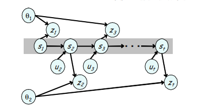
The SLAM problem can be described best as a probabilistic Markov chain. A graphical depiction of this Markov chain is shown in Figure 2.2. The current pose of the robot $s_{t}$ can be written as a probabilistic function of the pose at the previous time step $s_{t-1}$ and the control $u_{t}$ executed by the robot. This function is referred to as the motion model because it describes how controls drive the motion of the robot. Additionally, the motion model describes how noise in the controls injects uncertainty into the robot’s pose estimate. The motion model is written as:
$$
p\left(s_{t} \mid s_{t-1}, u_{t}\right)
$$
Sensor observations gathered by the robot are also governed by a probabilistic function, commonly referred to as the measurement model. The observation $z_{t}$
is a function of the observed landmark $\theta_{n_{t}}$ and the pose of the robot $s_{t}$. The measurement model describes the physics and the error model of the robot’s sensor. The measurement model is written as:
$$
p\left(z_{t} \mid s_{t}, \Theta, n_{t}\right)
$$
Using the motion model and the measurement model, the SLAM posterior at time $t$ can be computed recursively as function of the posterior at time $t-1$. This recursive update rule, known as the Bayes filter for SLAM, is the basis for the majority of online SLAM algorithms.
robotics代写|SLAM定位算法代写Simultaneous Localization and Mapping|Bayes Filter Derivation
The Bayes Filter can be derived from the SLAM posterior as follows. First, the posterior (2.6) is rewritten using Bayes Rule.
$$
p\left(s_{t}, \Theta \mid z^{t}, u^{t}, n^{t}\right)=\eta p\left(z_{t} \mid s_{t}, \Theta, z^{t-1}, u^{t}, n^{t}\right) p\left(s_{t}, \Theta \mid z^{t-1}, u^{t}, n^{t}\right)
$$
The denominator from Bayes rule is a normalizing constant and is written as $\eta$. Next, we exploit the fact that $z_{t}$ is solely a function of the pose of the robot $s_{t}$, the map $\Theta$, and the latest data association $n_{t}$, previously described as the measurement model. Hence the posterior becomes:
$$
=\eta p\left(z_{t} \mid s_{t}, \Theta, n_{t}\right) p\left(s_{t}, \Theta \mid z^{t-1}, u^{t}, n^{t}\right)
$$
Now we use the Theorem of Total Probability to condition the rightmost term of $(2.10)$ on the pose of the robot at time $t-1$.
$$
=\eta p\left(z_{t} \mid s_{t}, \Theta, n_{t}\right) \int p\left(s_{t}, \Theta \mid s_{t-1}, z^{t-1}, u^{t}, n^{t}\right) p\left(s_{t-1} \mid z^{t-1}, u^{t}, n^{t}\right) d s_{t-1}
$$
The leftmost term inside the integral can be expanded using the definition of conditional probability.
$$
\begin{aligned}
&=\eta p\left(z_{t} \mid s_{t}, \Theta, n_{t}\right) \
&\int p\left(s_{t} \mid \Theta, s_{t-1}, z^{t-1}, u^{t}, n^{t}\right) p\left(\Theta \mid s_{t-1}, z^{t-1}, u^{t}, n^{t}\right) p\left(s_{t-1} \mid z^{t-1}, u^{t}, n^{t}\right) d s_{t-1}
\end{aligned}
$$
The first term inside the integral can now be simplified by noting that $s_{t}$ is only a function of $s_{t-1}$ and $u_{t}$, previously described as the motion model.
$$
\begin{aligned}
&=\eta p\left(z_{t} \mid s_{t}, \Theta, n_{t}\right) \
&\qquad \int p\left(s_{t} \mid s_{t-1}, u_{t}\right) p\left(\Theta \mid s_{t-1}, z^{t-1}, u^{t}, n^{t}\right) p\left(s_{t-1} \mid z^{t-1}, u^{t}, n^{t}\right) d s_{t-1}
\end{aligned}
$$
At this point, the two rightmost terms in the integral can be combined.
$$
=\eta p\left(z_{t} \mid s_{t}, \Theta, n_{t}\right) \int p\left(s_{t} \mid s_{t-1}, u_{t}\right) p\left(s_{t-1}, \Theta \mid z^{t-1}, u^{t}, n^{t}\right) d s_{t-1}
$$
Since the current pose $u_{t}$ and data association $n_{t}$ provide no new information about $s_{t-1}$ or $\Theta$ without the latest observation $z_{t}$, they can be dropped from the rightmost term of the integral. The result is a recursive formula for computing the SLAM posterior at time $t$ given the SLAM posterior at time $t-1$, the motion model $p\left(s_{t} \mid s_{t-1}, u_{t}\right)$, and the measurement model $p\left(z_{t} \mid s_{t}, \Theta, n_{t}\right)$.
$$
\begin{aligned}
&p\left(s_{t}, \Theta \mid z^{t}, u^{t}, n^{t}\right)= \
&\eta p\left(z_{t} \mid s_{t}, \Theta, n_{t}\right) \int p\left(s_{t} \mid s_{t-1}, u_{t}\right) p\left(s_{t-1}, \Theta \mid z^{t-1}, u^{t-1}, n^{t-1}\right) d s_{t-1}
\end{aligned}
$$
SLAM定位算法代写
robotics代写|SLAM定位算法代写Simultaneous Localization and Mapping|SLAM Posterior
机器人当时的姿势吨将表示s吨. 对于在平面环境中运行的机器人,该位姿由机器人的X−是在平面上的位置及其航向。本书中介绍的所有实验结果都是在平面环境中生成的,但是算法同样适用于三维世界。机器人的完整轨迹,包括机器人在每个时间步的位姿,将被写为s吨.
s^{t}=\left{s_{1}, s_{2}, \ldots, s_{t}\right}s^{t}=\left{s_{1}, s_{2}, \ldots, s_{t}\right}
我们将进一步假设机器人的环境可以建模为一组ñ不动,点地标。点地标通常用于表示从传感器数据中提取的特征的位置,例如激光扫描中的几何特征或相机图像中的独特视觉特征。该组ñ地标位置将被写入\left{\theta_{1}, \ldots, \theta_{N}\right}\left{\theta_{1}, \ldots, \theta_{N}\right}. 为了符号简单,整个地图将被写为θ.
当机器人在环境中移动时,它会收集有关其自身运动的相关信息。这些信息可以使用附在机器人轮子上的里程表、惯性导航单元或简单地通过观察机器人执行的控制命令来生成。无论起源如何,对机器人运动的任何测量都将统称为控制。当时的控制吨会写在吨. 机器人执行的所有控制的集合将被写入在吨.
u^{t}=\left{u_{1}, u_{2}, \ldots, u_{t}\right}u^{t}=\left{u_{1}, u_{2}, \ldots, u_{t}\right}
当机器人在其环境中移动时,它会观察附近的地标。在平面 SLAM 问题的最常见公式中,机器人观察到附近障碍物的范围和方位。当时的观察吨会写和吨. 机器人收集的所有观测值的集合将被写入和吨.
z^{t}=\left{z_{1}, z_{2}, \ldots, z_{t}\right}z^{t}=\left{z_{1}, z_{2}, \ldots, z_{t}\right}
在 SLAM 文献中通常假设传感器测量可以分解为有关单个地标的信息,这样每个地标观察可以独立于其他测量值合并。在几乎所有成功的 SLAM 实现中,这是一个现实的假设,其中地标特征是从原始传感器数据中一一提取的。因此,我们将假设每个观测都提供了关于恰好一个地标位置的信息θn相对于机器人的当前姿势s吨. 变量n表示被观察的地标的身份。在实践中,通常无法观察到地标的身份,因为许多地标可能看起来很相似。与观测对应的地标的身份和吨将被写为n吨, 在哪里n吨∈1,…,ñ. 例如,n8=3意味着当时吨=8机器人观察到了第三个地标。地标身份通常被称为“数据关联”或“通信”。将写入所有数据关联的集合n吨.
n^{t}=\left{n_{1}, n_{2}, \ldots, n_{t}\right}n^{t}=\left{n_{1}, n_{2}, \ldots, n_{t}\right}
再次为简单起见,我们将假设机器人只接收一次测量值和吨并且只执行一个控件在吨每个时间步。每个时间步的多个观测值可以按顺序处理,但这会导致更繁琐的表示法。
使用上面定义的符号,SLAM 的主要目标是恢复机器人姿态的最佳估计s吨和地图θ,给定一组嘈杂的观测值和吨和控制在吨. 在概率方面,这由以下后验表示:
p(s吨,θ∣和吨,在吨)
如果数据关联集n吨同样给出,后验可以重写为:
p(s吨,θ∣和吨,在吨,n吨)
robotics代写|SLAM定位算法代写Simultaneous Localization and Mapping|SLAM as a Markov Chain
SLAM 问题可以最好地描述为概率马尔可夫链。该马尔可夫链的图形描述如图 2.2 所示。机器人当前位姿s吨可以写成前一个时间步的位姿的概率函数s吨−1和控制在吨由机器人执行。这个函数被称为运动模型,因为它描述了控制如何驱动机器人的运动。此外,运动模型描述了控制中的噪声如何将不确定性注入到机器人的姿态估计中。运动模型写为:
p(s吨∣s吨−1,在吨)
机器人收集的传感器观察结果也受概率函数控制,通常称为测量模型。观察和吨
是观察到的地标的函数θn吨和机器人的姿势s吨. 测量模型描述了机器人传感器的物理特性和误差模型。测量模型写为:
p(和吨∣s吨,θ,n吨)
使用运动模型和测量模型,SLAM 后验时间吨可以递归地计算为时间的后验函数吨−1. 这种递归更新规则,称为 SLAM 的贝叶斯过滤器,是大多数在线 SLAM 算法的基础。
robotics代写|SLAM定位算法代写Simultaneous Localization and Mapping|Bayes Filter Derivation
贝叶斯滤波器可以从 SLAM 后验推导出来,如下所示。首先,使用贝叶斯规则重写后验(2.6)。
p(s吨,θ∣和吨,在吨,n吨)=这p(和吨∣s吨,θ,和吨−1,在吨,n吨)p(s吨,θ∣和吨−1,在吨,n吨)
贝叶斯规则的分母是归一化常数,写为这. 接下来,我们利用以下事实和吨仅是机器人姿态的函数s吨, 地图θ,以及最新的数据关联n吨,之前描述为测量模型。因此后验变为:
=这p(和吨∣s吨,θ,n吨)p(s吨,θ∣和吨−1,在吨,n吨)
现在我们使用总概率定理来调节最右边的项(2.10)关于机器人当时的位姿吨−1.
=这p(和吨∣s吨,θ,n吨)∫p(s吨,θ∣s吨−1,和吨−1,在吨,n吨)p(s吨−1∣和吨−1,在吨,n吨)ds吨−1
积分内最左边的项可以使用条件概率的定义进行扩展。
=这p(和吨∣s吨,θ,n吨) ∫p(s吨∣θ,s吨−1,和吨−1,在吨,n吨)p(θ∣s吨−1,和吨−1,在吨,n吨)p(s吨−1∣和吨−1,在吨,n吨)ds吨−1
积分内的第一项现在可以简化为:s吨只是一个函数s吨−1和在吨,之前描述为运动模型。
=这p(和吨∣s吨,θ,n吨) ∫p(s吨∣s吨−1,在吨)p(θ∣s吨−1,和吨−1,在吨,n吨)p(s吨−1∣和吨−1,在吨,n吨)ds吨−1
此时,积分中最右边的两项可以合并。
=这p(和吨∣s吨,θ,n吨)∫p(s吨∣s吨−1,在吨)p(s吨−1,θ∣和吨−1,在吨,n吨)ds吨−1
由于当前姿势在吨和数据关联n吨不提供有关的新信息s吨−1或者θ没有最新的观察和吨,它们可以从积分的最右边项中删除。结果是用于计算 SLAM 后验的递归公式吨给定 SLAM 后验时间吨−1, 运动模型p(s吨∣s吨−1,在吨), 和测量模型p(和吨∣s吨,θ,n吨).
p(s吨,θ∣和吨,在吨,n吨)= 这p(和吨∣s吨,θ,n吨)∫p(s吨∣s吨−1,在吨)p(s吨−1,θ∣和吨−1,在吨−1,n吨−1)ds吨−1

统计代写请认准statistics-lab™. statistics-lab™为您的留学生涯保驾护航。
金融工程代写
金融工程是使用数学技术来解决金融问题。金融工程使用计算机科学、统计学、经济学和应用数学领域的工具和知识来解决当前的金融问题,以及设计新的和创新的金融产品。
非参数统计代写
非参数统计指的是一种统计方法,其中不假设数据来自于由少数参数决定的规定模型;这种模型的例子包括正态分布模型和线性回归模型。
广义线性模型代考
广义线性模型(GLM)归属统计学领域,是一种应用灵活的线性回归模型。该模型允许因变量的偏差分布有除了正态分布之外的其它分布。
术语 广义线性模型(GLM)通常是指给定连续和/或分类预测因素的连续响应变量的常规线性回归模型。它包括多元线性回归,以及方差分析和方差分析(仅含固定效应)。
有限元方法代写
有限元方法(FEM)是一种流行的方法,用于数值解决工程和数学建模中出现的微分方程。典型的问题领域包括结构分析、传热、流体流动、质量运输和电磁势等传统领域。
有限元是一种通用的数值方法,用于解决两个或三个空间变量的偏微分方程(即一些边界值问题)。为了解决一个问题,有限元将一个大系统细分为更小、更简单的部分,称为有限元。这是通过在空间维度上的特定空间离散化来实现的,它是通过构建对象的网格来实现的:用于求解的数值域,它有有限数量的点。边界值问题的有限元方法表述最终导致一个代数方程组。该方法在域上对未知函数进行逼近。[1] 然后将模拟这些有限元的简单方程组合成一个更大的方程系统,以模拟整个问题。然后,有限元通过变化微积分使相关的误差函数最小化来逼近一个解决方案。
tatistics-lab作为专业的留学生服务机构,多年来已为美国、英国、加拿大、澳洲等留学热门地的学生提供专业的学术服务,包括但不限于Essay代写,Assignment代写,Dissertation代写,Report代写,小组作业代写,Proposal代写,Paper代写,Presentation代写,计算机作业代写,论文修改和润色,网课代做,exam代考等等。写作范围涵盖高中,本科,研究生等海外留学全阶段,辐射金融,经济学,会计学,审计学,管理学等全球99%专业科目。写作团队既有专业英语母语作者,也有海外名校硕博留学生,每位写作老师都拥有过硬的语言能力,专业的学科背景和学术写作经验。我们承诺100%原创,100%专业,100%准时,100%满意。
随机分析代写
随机微积分是数学的一个分支,对随机过程进行操作。它允许为随机过程的积分定义一个关于随机过程的一致的积分理论。这个领域是由日本数学家伊藤清在第二次世界大战期间创建并开始的。
时间序列分析代写
随机过程,是依赖于参数的一组随机变量的全体,参数通常是时间。 随机变量是随机现象的数量表现,其时间序列是一组按照时间发生先后顺序进行排列的数据点序列。通常一组时间序列的时间间隔为一恒定值(如1秒,5分钟,12小时,7天,1年),因此时间序列可以作为离散时间数据进行分析处理。研究时间序列数据的意义在于现实中,往往需要研究某个事物其随时间发展变化的规律。这就需要通过研究该事物过去发展的历史记录,以得到其自身发展的规律。
回归分析代写
多元回归分析渐进(Multiple Regression Analysis Asymptotics)属于计量经济学领域,主要是一种数学上的统计分析方法,可以分析复杂情况下各影响因素的数学关系,在自然科学、社会和经济学等多个领域内应用广泛。
MATLAB代写
MATLAB 是一种用于技术计算的高性能语言。它将计算、可视化和编程集成在一个易于使用的环境中,其中问题和解决方案以熟悉的数学符号表示。典型用途包括:数学和计算算法开发建模、仿真和原型制作数据分析、探索和可视化科学和工程图形应用程序开发,包括图形用户界面构建MATLAB 是一个交互式系统,其基本数据元素是一个不需要维度的数组。这使您可以解决许多技术计算问题,尤其是那些具有矩阵和向量公式的问题,而只需用 C 或 Fortran 等标量非交互式语言编写程序所需的时间的一小部分。MATLAB 名称代表矩阵实验室。MATLAB 最初的编写目的是提供对由 LINPACK 和 EISPACK 项目开发的矩阵软件的轻松访问,这两个项目共同代表了矩阵计算软件的最新技术。MATLAB 经过多年的发展,得到了许多用户的投入。在大学环境中,它是数学、工程和科学入门和高级课程的标准教学工具。在工业领域,MATLAB 是高效研究、开发和分析的首选工具。MATLAB 具有一系列称为工具箱的特定于应用程序的解决方案。对于大多数 MATLAB 用户来说非常重要,工具箱允许您学习和应用专业技术。工具箱是 MATLAB 函数(M 文件)的综合集合,可扩展 MATLAB 环境以解决特定类别的问题。可用工具箱的领域包括信号处理、控制系统、神经网络、模糊逻辑、小波、仿真等。