如果你也在 怎样代写图论Graph Theory 这个学科遇到相关的难题，请随时右上角联系我们的24/7代写客服。图论Graph Theory有趣的部分原因在于，图可以用来对某些问题中的情况进行建模。这些问题可以在图表的帮助下进行研究(并可能得到解决)。因此，图形模型在本书中经常出现。然而，图论是数学的一个领域，因此涉及数学思想的研究-概念和它们之间的联系。我们选择包含的主题和结果是因为我们认为它们有趣、重要和/或代表主题。

图论Graph Theory通过熟悉许多过去和现在对图论的发展负责的人，可以增强对图论的欣赏。因此，我们收录了一些关于“图论人士”的有趣评论。因为我们相信这些人是图论故事的一部分，所以我们在文中讨论了他们，而不仅仅是作为脚注。我们常常没有认识到数学是一门有生命的学科。图论是人类创造的，是一门仍在不断发展的学科。

statistics-lab™ 为您的留学生涯保驾护航 在代写图论Graph Theory方面已经树立了自己的口碑, 保证靠谱, 高质且原创的统计Statistics代写服务。我们的专家在代写图论Graph Theory代写方面经验极为丰富，各种代写图论Graph Theory相关的作业也就用不着说。

数学代写|图论作业代写Graph Theory代考|Ramsey properties and connectivity

According to Ramsey’s theorem, every large enough graph $G$ has a very dense or a very sparse induced subgraph of given order, a $K^r$ or $\overline{K^r}$. If we assume that $G$ is connected, we can say a little more:

Proposition 9.4.1. For every $r \in \mathbb{N}$ there is an $n \in \mathbb{N}$ such that every connected graph of order at least $n$ contains $K^r, K_{1, r}$ or $P^r$ as an induced subgraph.

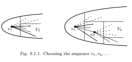
Proof. Let $d+1$ be the Ramsey number of $r$, let $n:=\frac{d}{d-2}(d-1)^r$, and let $G$ be a graph of order at least $n$. If $G$ has a vertex $v$ of degree at least $d+1$ then, by Theorem 9.1.1 and the choice of $d$, either $N(v)$ induces a $K^r$ in $G$ or ${v} \cup N(v)$ induces a $K_{1, r}$. On the other hand, if $\Delta(G) \leqslant d$, then by Proposition 1.3.3 $G$ has radius $>r$, and hence contains two vertices at a distance $\geqslant r$. Any shortest path in $G$ between these two vertices contains a $P^r$.

In principle, we could now look for a similar set of ‘unavoidable’ $k$-connected subgraphs for any given connectivity $k$. To keep thse ‘unavoidable sets’ small, it helps to relax the containment relation from ‘induced subgraph’ for $k=1$ (as above) to ‘topological minor’ for $k=2$, and on to ‘minor’ for $k=3$ and $k=4$. For larger $k$, no similar results are known.

Proposition 9.4.2. For every $r \in \mathbb{N}$ there is an $n \in \mathbb{N}$ such that every 2-connected graph of order at least $n$ contains $C^r$ or $K_{2, r}$ as a topological minor.

Proof. Let $d$ be the $n$ associated with $r$ in Proposition 9.4.1, and let $G$ be a 2-connected graph with at least $\frac{d}{d-2}(d-1)^r$ vertices. By Proposition 1.3.3, either $G$ has a vertex of degree $>d$ or $\operatorname{diam} G \geqslant \operatorname{rad} G>r$.

In the latter case let $a, b \in G$ be two vertices at distance $>r$. By Menger’s theorem (3.3.6), $G$ contains two independent $a-b$ paths. These form a cycle of length $>r$.

数学代写|图论作业代写Graph Theory代考|Simple sufficient conditions

What kind of condition might be sufficient for the existence of a Hamilton cycle in a graph $G$ ? Purely global assumptions, like high edge density, will not be enough: we cannot do without the local property that every vertex has at least two neighbours. But neither is any large (but constant) minimum degree sufficient: it is easy to find graphs without a Hamilton cycle whose minimum degree exceeds any given constant bound.
The following classic result derives its significance from this background:

Theorem 10.1.1. (Dirac 1952)
Every graph with $n \geqslant 3$ vertices and minimum degree at least $n / 2$ has a Hamilton cycle.

Proof. Let $G=(V, E)$ be a graph with $|G|=n \geqslant 3$ and $\delta(G) \geqslant n / 2$. Then $G$ is connected: otherwise, the degree of any vertex in the smallest component $C$ of $G$ would be less than $|C| \leqslant n / 2$.

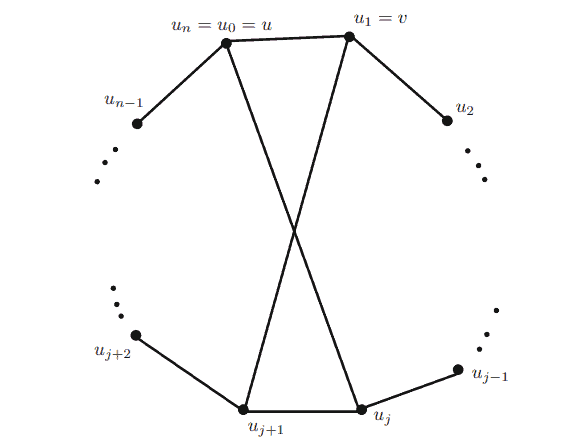
Let $P=x_0 \ldots x_k$ be a longest path in $G$. By the maximality of $P$, all the neighbours of $x_0$ and all the neighbours of $x_k$ lie on $P$. Hence at least $n / 2$ of the vertices $x_0, \ldots, x_{k-1}$ are adjacent to $x_k$, and at least $n / 2$ of these same $k<n$ vertices $x_i$ are such that $x_0 x_{i+1} \in E$. By the pigeon hole principle, there is a vertex $x_i$ that has both properties, so we have $x_0 x_{i+1} \in E$ and $x_i x_k \in E$ for some $i<k$ (Fig. 10.1.1).

We claim that the cycle $C:=x_0 x_{i+1} P x_k x_i P x_0$ is a Hamilton cycle of $G$. Indeed, since $G$ is connected, $C$ would otherwise have a neighbour in $G-C$, which could be combined with a spanning path of $C$ into a path longer than $P$.

图论代考

数学代写|图论作业代写Graph Theory代考|Ramsey properties and connectivity

根据拉姆齐定理，每个足够大的图$G$都有一个非常密集或非常稀疏的给定阶的诱导子图$K^r$或$\overline{K^r}$。如果我们假设$G$是连接的，我们可以多说一点:

提案9.4.1对于每个$r \in \mathbb{N}$，都存在一个$n \in \mathbb{N}$，使得每个至少为$n$阶的连通图都包含$K^r, K_{1, r}$或$P^r$作为诱导子图。

证明。设$d+1$为$r$的拉姆齐数，设$n:=\frac{d}{d-2}(d-1)^r$，设$G$为至少为$n$的有序图。如果$G$有一个顶点$v$的度数至少为$d+1$，那么根据定理9.1.1和$d$的选择，要么$N(v)$在$G$中衍生出一个$K^r$，要么${v} \cup N(v)$衍生出一个$K_{1, r}$。另一方面，如果$\Delta(G) \leqslant d$，则根据命题1.3.3 $G$的半径为$>r$，因此包含两个距离为$\geqslant r$的顶点。在$G$中这两个顶点之间的任何最短路径都包含$P^r$。

原则上，对于任何给定的连通性$k$，我们现在可以寻找类似的一组“不可避免的”$k$连接子图。为了保持这些“不可避免的集合”较小，它有助于将包含关系从$k=1$的“诱导子图”(如上所述)放宽到$k=2$的“拓扑次要”，然后再放宽到$k=3$和$k=4$的“次要”。对于更大的$k$，没有类似的结果。

提案9.4.2。对于每个$r \in \mathbb{N}$，都存在一个$n \in \mathbb{N}$，使得每个至少为$n$阶的2连通图都包含$C^r$或$K_{2, r}$作为拓扑次元。

证明。设$d$为命题9.4.1中与$r$相关联的$n$，设$G$为至少有$\frac{d}{d-2}(d-1)^r$个顶点的2连通图。根据命题1.3.3,$G$有一个度数为$>d$或$\operatorname{diam} G \geqslant \operatorname{rad} G>r$的顶点。

在后一种情况下，设$a, b \in G$为距离为$>r$的两个顶点。根据门格尔定理(3.3.6)，$G$包含两个独立的$a-b$路径。这些形成了一个长度为$>r$的循环。

数学代写|图论作业代写Graph Theory代考|Simple sufficient conditions

什么样的条件可能是图中存在汉密尔顿环的充分条件$G$ ?纯粹的全局假设，比如高边缘密度，是不够的:我们不能没有每个顶点至少有两个邻居的局部性质。但是，任何大的(但恒定的)最小度都是不够的:很容易找到没有Hamilton循环的图，其最小度超过任何给定的常数界。
下面这个经典结论的意义就来源于这个背景:

定理10.1.1。(狄拉克1952)
每个顶点为$n \geqslant 3$且最小度至少为$n / 2$的图都有一个Hamilton循环。

证明。设$G=(V, E)$为具有$|G|=n \geqslant 3$和$\delta(G) \geqslant n / 2$的图形。那么$G$是连通的，否则$G$的最小分量$C$中任意顶点的度数都小于$|C| \leqslant n / 2$。

设$P=x_0 \ldots x_k$为$G$的最长路径。根据$P$的最大值，$x_0$的所有邻居和$x_k$的所有邻居都在$P$上。因此，至少$n / 2$个顶点$x_0, \ldots, x_{k-1}$与$x_k$相邻，并且至少$n / 2$个相同的$k<n$个顶点$x_i$与$x_0 x_{i+1} \in E$相邻。根据鸽子洞原理，有一个顶点$x_i$同时具有这两个属性，因此对于某些$i<k$，我们有$x_0 x_{i+1} \in E$和$x_i x_k \in E$(图10.1.1)。

我们声称周期$C:=x_0 x_{i+1} P x_k x_i P x_0$是一个$G$的汉密尔顿周期。事实上，因为$G$是连通的，否则$C$在$G-C$中就会有一个邻居，它可以与$C$的生成路径组合成一条比$P$长的路径。

统计代写请认准statistics-lab™. statistics-lab™为您的留学生涯保驾护航。

微观经济学代写

微观经济学是主流经济学的一个分支，研究个人和企业在做出有关稀缺资源分配的决策时的行为以及这些个人和企业之间的相互作用。my-assignmentexpert™ 为您的留学生涯保驾护航 在数学Mathematics作业代写方面已经树立了自己的口碑, 保证靠谱, 高质且原创的数学Mathematics代写服务。我们的专家在图论代写Graph Theory代写方面经验极为丰富，各种图论代写Graph Theory相关的作业也就用不着 说。

线性代数代写

线性代数是数学的一个分支，涉及线性方程，如：线性图，如：以及它们在向量空间和通过矩阵的表示。线性代数是几乎所有数学领域的核心。

博弈论代写

现代博弈论始于约翰-冯-诺伊曼（John von Neumann）提出的两人零和博弈中的混合策略均衡的观点及其证明。冯-诺依曼的原始证明使用了关于连续映射到紧凑凸集的布劳威尔定点定理，这成为博弈论和数学经济学的标准方法。在他的论文之后，1944年，他与奥斯卡-莫根斯特恩（Oskar Morgenstern）共同撰写了《游戏和经济行为理论》一书，该书考虑了几个参与者的合作游戏。这本书的第二版提供了预期效用的公理理论，使数理统计学家和经济学家能够处理不确定性下的决策。

微积分代写

微积分，最初被称为无穷小微积分或 “无穷小的微积分”，是对连续变化的数学研究，就像几何学是对形状的研究，而代数是对算术运算的概括研究一样。

它有两个主要分支，微分和积分；微分涉及瞬时变化率和曲线的斜率，而积分涉及数量的累积，以及曲线下或曲线之间的面积。这两个分支通过微积分的基本定理相互联系，它们利用了无限序列和无限级数收敛到一个明确定义的极限的基本概念 。

计量经济学代写

什么是计量经济学？
计量经济学是统计学和数学模型的定量应用，使用数据来发展理论或测试经济学中的现有假设，并根据历史数据预测未来趋势。它对现实世界的数据进行统计试验，然后将结果与被测试的理论进行比较和对比。

根据你是对测试现有理论感兴趣，还是对利用现有数据在这些观察的基础上提出新的假设感兴趣，计量经济学可以细分为两大类：理论和应用。那些经常从事这种实践的人通常被称为计量经济学家。

Matlab代写

MATLAB 是一种用于技术计算的高性能语言。它将计算、可视化和编程集成在一个易于使用的环境中，其中问题和解决方案以熟悉的数学符号表示。典型用途包括：数学和计算算法开发建模、仿真和原型制作数据分析、探索和可视化科学和工程图形应用程序开发，包括图形用户界面构建MATLAB 是一个交互式系统，其基本数据元素是一个不需要维度的数组。这使您可以解决许多技术计算问题，尤其是那些具有矩阵和向量公式的问题，而只需用 C 或 Fortran 等标量非交互式语言编写程序所需的时间的一小部分。MATLAB 名称代表矩阵实验室。MATLAB 最初的编写目的是提供对由 LINPACK 和 EISPACK 项目开发的矩阵软件的轻松访问，这两个项目共同代表了矩阵计算软件的最新技术。MATLAB 经过多年的发展，得到了许多用户的投入。在大学环境中，它是数学、工程和科学入门和高级课程的标准教学工具。在工业领域，MATLAB 是高效研究、开发和分析的首选工具。MATLAB 具有一系列称为工具箱的特定于应用程序的解决方案。对于大多数 MATLAB 用户来说非常重要，工具箱允许您学习和应用专业技术。工具箱是 MATLAB 函数（M 文件）的综合集合，可扩展 MATLAB 环境以解决特定类别的问题。可用工具箱的领域包括信号处理、控制系统、神经网络、模糊逻辑、小波、仿真等。

如果你也在 怎样代写图论Graph Theory 这个学科遇到相关的难题，请随时右上角联系我们的24/7代写客服。图论Graph Theory有趣的部分原因在于，图可以用来对某些问题中的情况进行建模。这些问题可以在图表的帮助下进行研究(并可能得到解决)。因此，图形模型在本书中经常出现。然而，图论是数学的一个领域，因此涉及数学思想的研究-概念和它们之间的联系。我们选择包含的主题和结果是因为我们认为它们有趣、重要和/或代表主题。

图论Graph Theory通过熟悉许多过去和现在对图论的发展负责的人，可以增强对图论的欣赏。因此，我们收录了一些关于“图论人士”的有趣评论。因为我们相信这些人是图论故事的一部分，所以我们在文中讨论了他们，而不仅仅是作为脚注。我们常常没有认识到数学是一门有生命的学科。图论是人类创造的，是一门仍在不断发展的学科。

statistics-lab™ 为您的留学生涯保驾护航 在代写图论Graph Theory方面已经树立了自己的口碑, 保证靠谱, 高质且原创的统计Statistics代写服务。我们的专家在代写图论Graph Theory代写方面经验极为丰富，各种代写图论Graph Theory相关的作业也就用不着说。

数学代写|图论作业代写Graph Theory代考|Ramsey numbers

Ramsey’s theorem may be rephrased as follows: if $H=K^r$ and $G$ is a graph with sufficiently many vertices, then either $G$ itself or its complement $\bar{G}$ contains a copy of $H$ as a subgraph. Clearly, the same is true for any graph $H$, simply because $H \subseteq K^h$ for $h:=|H|$.

However, if we ask for the least $n$ such that every graph $G$ of order $n$ has the above property – this is the Ramsey number $R(H)$ of $H$-then the above question makes sense: if $H$ has only few edges, it should embed more easily in $G$ or $\bar{G}$, and we would expect $R(H)$ to be smaller than the Ramsey number $R(h)=R\left(K^h\right)$.

A little more generally, let $R\left(H_1, H_2\right)$ denote the least $n \in \mathbb{N}$ such that $H_1 \subseteq G$ or $H_2 \subseteq \bar{G}$ for every graph $G$ of order $n$. For most graphs $H_1, H_2$, only very rough estimates are known for $R\left(H_1, H_2\right)$. Interestingly, lower bounds given by random graphs (as in Theorem 11.1.3) are often sharper than even the best bounds provided by explicit constructions.

The following proposition describes one of the few cases where exact Ramsey numbers are known for a relatively large class of graphs:

Proposition 9.2.1. Let $s, t$ be positive integers, and let $T$ be a tree of order $t$. Then $R\left(T, K^s\right)=(s-1)(t-1)+1$.

Proof. The disjoint union of $s-1$ graphs $K^{t-1}$ contains no copy of $T$, while the complement of this graph, the complete $(s-1)$-partite graph $K_{t-1}^{s-1}$, does not contain $K^s$. This proves $R\left(T, K^s\right) \geqslant(s-1)(t-1)+1$.
Conversely, let $G$ be any graph of order $n=(s-1)(t-1)+1$ whose complement contains no $K^s$. Then $s>1$, and in any vertex colouring of $G$ (in the sense of Chapter 5) at most $s-1$ vertices can have the same colour. Hence, $\chi(G) \geqslant\lceil n /(s-1)\rceil=t$. By Corollary $5.2 .3, G$ has a subgraph $H$ with $\delta(H) \geqslant t-1$, which by Corollary 1.5 .4 contains a copy of $T$.

数学代写|图论作业代写Graph Theory代考|Induced Ramsey theorems

Ramsey’s theorem can be rephrased as follows. For every graph $H=K^r$ there exists a graph $G$ such that every 2-colouring of the edges of $G$ yields a monochromatic $H \subseteq G$; as it turns out, this is witnessed by any large enough complete graph as $G$. Let us now change the problem slightly and ask for a graph $G$ in which every 2-edge-colouring yields a monochromatic induced $H \subseteq G$, where $H$ is now an arbitrary given graph.

This slight modification changes the character of the problem dramatically. What is needed now is no longer a simple proof that $G$ is ‘big enough’ (as for Theorem 9.1.1), but a careful construction: the construction of a graph that, however we bipartition its edges, contains an induced copy of $H$ with all edges in one partition class. We shall call such a graph a Ramsey graph for $H$.

The fact that such a Ramsey graph exists for every choice of $H$ is one of the fundamental results of graph Ramsey theory. It was proved around 1973 , independently by Deuber, by Erdős, Hajnal \& Pósa, and by Rödl.

Theorem 9.3.1. Every graph has a Ramsey graph. In other words, for every graph $H$ there exists a graph $G$ that, for every partition $\left{E_1, E_2\right}$ of $E(G)$, has an induced subgraph $H$ with $E(H) \subseteq E_1$ or $E(H) \subseteq E_2$.

We give two proofs. Each of these is highly individual, yet each offers a glimpse of true Ramsey theory: the graphs involved are used as hardly more than bricks in the construction, but the edifice is impressive.

图论代考

数学代写|图论作业代写Graph Theory代考|Ramsey numbers

拉姆齐定理可以重新表述如下:如果$H=K^r$和$G$是一个具有足够多顶点的图，那么$G$本身或它的补$\bar{G}$包含一个$H$的副本作为子图。显然，对于任何图形$H$都是一样的，因为$H \subseteq K^h$对于$h:=|H|$。

然而，如果我们要求最小的$n$，使得$n$的每个图$G$都具有上述属性——这是$H$的拉姆齐数$R(H)$——那么上面的问题就有意义了:如果$H$只有几个边，它应该更容易嵌入到$G$或$\bar{G}$中，我们会期望$R(H)$比拉姆齐数$R(h)=R\left(K^h\right)$小。

更一般地说，让$R\left(H_1, H_2\right)$表示最小的$n \in \mathbb{N}$，使得$H_1 \subseteq G$或$H_2 \subseteq \bar{G}$对于每个顺序为$n$的图$G$。对于大多数图形$H_1, H_2$，对于$R\left(H_1, H_2\right)$只有非常粗略的估计。有趣的是，随机图给出的下界(如定理11.1.3)往往比显式构造提供的最佳边界更清晰。

下面的命题描述了为数不多的情况之一，其中确切的拉姆齐数是已知的相对较大的一类图:

提案9.2.1设$s, t$为正整数，设$T$为$t$阶的树。然后$R\left(T, K^s\right)=(s-1)(t-1)+1$。

证明。$s-1$图的不相交并$K^{t-1}$不包含$T$的副本，而这个图的补图，完整的$(s-1)$ -部图$K_{t-1}^{s-1}$，不包含$K^s$。这证明了$R\left(T, K^s\right) \geqslant(s-1)(t-1)+1$。
反之，设$G$为任意阶为$n=(s-1)(t-1)+1$的图，其补不包含$K^s$。然后$s>1$，在$G$的任何顶点着色中(在第5章的意义上)，最多$s-1$个顶点可以具有相同的颜色。因此，$\chi(G) \geqslant\lceil n /(s-1)\rceil=t$。根据推论$5.2 .3, G$与$\delta(H) \geqslant t-1$有一个子图$H$，根据推论1.5 .4,包含一个$T$的副本。

数学代写|图论作业代写Graph Theory代考|Induced Ramsey theorems

拉姆齐定理可以改写如下。对于每个图$H=K^r$，存在一个图$G$，使得$G$的每条边的2种颜色产生一个单色的$H \subseteq G$;事实证明，任何足够大的完全图都可以证明这一点，如$G$。现在让我们稍微改变一下问题，并要求一个图$G$，其中每个2边着色产生一个单色诱导$H \subseteq G$，其中$H$现在是一个任意给定的图。

这个微小的修改戏剧性地改变了问题的性质。现在需要的不再是一个简单的证明$G$“足够大”(如定理9.1.1)，而是一个仔细的构造:一个图的构造，无论我们如何划分它的边，都包含一个$H$的诱导副本，所有的边都在一个划分类中。我们称这种图为$H$的拉姆齐图。

对于每一个$H$的选择都存在这样的Ramsey图，这是图Ramsey理论的基本结果之一。大约在1973年，Deuber, Erdős, Hajnal ＆ Pósa和Rödl分别独立地证明了这一点。

定理9.3.1。每个图都有一个拉姆齐图。换句话说，对于每个图$H$，存在一个图$G$，对于$E(G)$的每个分区$\left{E_1, E_2\right}$，都有一个与$E(H) \subseteq E_1$或$E(H) \subseteq E_2$的诱导子图$H$。

我们给出了两个证明。每一个都是高度独立的，但每一个都提供了真正的拉姆齐理论的一瞥:所涉及的图表几乎与建筑中的砖块差不多，但这座大厦令人印象深刻。

统计代写请认准statistics-lab™. statistics-lab™为您的留学生涯保驾护航。

微观经济学代写

微观经济学是主流经济学的一个分支，研究个人和企业在做出有关稀缺资源分配的决策时的行为以及这些个人和企业之间的相互作用。my-assignmentexpert™ 为您的留学生涯保驾护航 在数学Mathematics作业代写方面已经树立了自己的口碑, 保证靠谱, 高质且原创的数学Mathematics代写服务。我们的专家在图论代写Graph Theory代写方面经验极为丰富，各种图论代写Graph Theory相关的作业也就用不着 说。

线性代数代写

线性代数是数学的一个分支，涉及线性方程，如：线性图，如：以及它们在向量空间和通过矩阵的表示。线性代数是几乎所有数学领域的核心。

博弈论代写

现代博弈论始于约翰-冯-诺伊曼（John von Neumann）提出的两人零和博弈中的混合策略均衡的观点及其证明。冯-诺依曼的原始证明使用了关于连续映射到紧凑凸集的布劳威尔定点定理，这成为博弈论和数学经济学的标准方法。在他的论文之后，1944年，他与奥斯卡-莫根斯特恩（Oskar Morgenstern）共同撰写了《游戏和经济行为理论》一书，该书考虑了几个参与者的合作游戏。这本书的第二版提供了预期效用的公理理论，使数理统计学家和经济学家能够处理不确定性下的决策。

微积分代写

微积分，最初被称为无穷小微积分或 “无穷小的微积分”，是对连续变化的数学研究，就像几何学是对形状的研究，而代数是对算术运算的概括研究一样。

它有两个主要分支，微分和积分；微分涉及瞬时变化率和曲线的斜率，而积分涉及数量的累积，以及曲线下或曲线之间的面积。这两个分支通过微积分的基本定理相互联系，它们利用了无限序列和无限级数收敛到一个明确定义的极限的基本概念 。

计量经济学代写

什么是计量经济学？
计量经济学是统计学和数学模型的定量应用，使用数据来发展理论或测试经济学中的现有假设，并根据历史数据预测未来趋势。它对现实世界的数据进行统计试验，然后将结果与被测试的理论进行比较和对比。

根据你是对测试现有理论感兴趣，还是对利用现有数据在这些观察的基础上提出新的假设感兴趣，计量经济学可以细分为两大类：理论和应用。那些经常从事这种实践的人通常被称为计量经济学家。

Matlab代写

MATLAB 是一种用于技术计算的高性能语言。它将计算、可视化和编程集成在一个易于使用的环境中，其中问题和解决方案以熟悉的数学符号表示。典型用途包括：数学和计算算法开发建模、仿真和原型制作数据分析、探索和可视化科学和工程图形应用程序开发，包括图形用户界面构建MATLAB 是一个交互式系统，其基本数据元素是一个不需要维度的数组。这使您可以解决许多技术计算问题，尤其是那些具有矩阵和向量公式的问题，而只需用 C 或 Fortran 等标量非交互式语言编写程序所需的时间的一小部分。MATLAB 名称代表矩阵实验室。MATLAB 最初的编写目的是提供对由 LINPACK 和 EISPACK 项目开发的矩阵软件的轻松访问，这两个项目共同代表了矩阵计算软件的最新技术。MATLAB 经过多年的发展，得到了许多用户的投入。在大学环境中，它是数学、工程和科学入门和高级课程的标准教学工具。在工业领域，MATLAB 是高效研究、开发和分析的首选工具。MATLAB 具有一系列称为工具箱的特定于应用程序的解决方案。对于大多数 MATLAB 用户来说非常重要，工具箱允许您学习和应用专业技术。工具箱是 MATLAB 函数（M 文件）的综合集合，可扩展 MATLAB 环境以解决特定类别的问题。可用工具箱的领域包括信号处理、控制系统、神经网络、模糊逻辑、小波、仿真等。

如果你也在 怎样代写图论Graph Theory 这个学科遇到相关的难题，请随时右上角联系我们的24/7代写客服。图论Graph Theory有趣的部分原因在于，图可以用来对某些问题中的情况进行建模。这些问题可以在图表的帮助下进行研究(并可能得到解决)。因此，图形模型在本书中经常出现。然而，图论是数学的一个领域，因此涉及数学思想的研究-概念和它们之间的联系。我们选择包含的主题和结果是因为我们认为它们有趣、重要和/或代表主题。

图论Graph Theory通过熟悉许多过去和现在对图论的发展负责的人，可以增强对图论的欣赏。因此，我们收录了一些关于“图论人士”的有趣评论。因为我们相信这些人是图论故事的一部分，所以我们在文中讨论了他们，而不仅仅是作为脚注。我们常常没有认识到数学是一门有生命的学科。图论是人类创造的，是一门仍在不断发展的学科。

statistics-lab™ 为您的留学生涯保驾护航 在代写图论Graph Theory方面已经树立了自己的口碑, 保证靠谱, 高质且原创的统计Statistics代写服务。我们的专家在代写图论Graph Theory代写方面经验极为丰富，各种代写图论Graph Theory相关的作业也就用不着说。

数学代写|图论作业代写Graph Theory代考|The topological end space

In this last section we shall develop a deeper understanding of the global structure of infinite graphs, especially locally finite ones, that can be attained only by studying their ends. This structure is intrinsically topological, but no more than the most basic concepts of point-set topology will be needed.

Our starting point will be to make precise the intuitive idea that the ends of a graph are the ‘points at infinity’ to which its rays converge. To do so, we shall define a topological space $|G|$ associated with a graph $G=(V, E, \Omega)$ and its ends. ${ }^8$ By considering topological versions of paths, cycles and spanning trees in this space, we shall then be able to extend to infinite graphs some parts of finite graph theory that would not otherwise have infinite counterparts (see the notes for more examples). Thus, the ends of an infinite graph turn out to be more than a curious new phenomenon: they form an integral part of the picture, without which it cannot be properly understood.

To build the space $|G|$ formally, we start with the set $V \cup \Omega$. For every edge $e=u v$ we add a set $\dot{e}=(u, v)$ of continuum many points, making these sets $\ddot{e}$ disjoint from each other and from $V \cup \Omega$. We then choose for each $e$ some fixed bijection between $\dot{e}$ and the real interval $(0,1)$, and extend this bijection to one between $[u, v]:={u} \cup \grave{e} \cup{v}$ and $[0,1]$. This bijection defines a metric on $[u, v]$; we call $[u, v]$ a topological edge with inner points $x \in \dot{e}$. Given any $F \subseteq E$ we write $\stackrel{\circ}{F}:=\bigcup{\dot{e} \mid e \in F}$.

When we speak of a ‘graph’ $H \subseteq G$, we shall often also mean its corresponding point set $V(H) \cup \tilde{E}(H)$.

Having thus defined the point set of $|G|$, let us choose a basis of open sets to define its topology. For every edge $u v$, declare as open all subsets of $(u, v)$ that correspond, by our fixed bijection between $(u, v)$ and $(0,1)$, to an open set in $(0,1)$. For every vertex $u$ and $\epsilon>0$, declare as open the ‘open star around $u$ of radius $\epsilon$ ‘, that is, the set of all points on edges $[u, v]$ at distance less than $\epsilon$ from $u$, measured individually for each edge in its metric inherited from $[0,1]$. Finally, for every end $\omega$ and every finite set $S \subseteq V$, there is a unique component $C(S, \omega)$ of $G-S$ that contains a ray from $\omega$. Let $\Omega(S, \omega):=\left{\omega^{\prime} \in \Omega \mid C\left(S, \omega^{\prime}\right)=C(S, \omega)\right}$. For every $\epsilon>0$, write $E_\epsilon(S, \omega)$ for the set of all inner points of $S$ $C(S, \omega)$ edges at distance less than $\epsilon$ from their endpoint in $C(S, \omega)$. Then declare as open all sets of the form
$$
\hat{C}\epsilon(S, \omega):=C(S, \omega) \cup \Omega(S, \omega) \cup \dot{E}\epsilon(S, \omega) .
$$

数学代写|图论作业代写Graph Theory代考|Ramsey’s original theorems

In its simplest version, Ramsey’s theorem says that, given an integer $r \geqslant 0$, every large enough graph $G$ contains either $K^r$ or $\overline{K^r}$ as an induced subgraph. At first glance, this may seem surprising: after all, we need about $(r-2) /(r-1)$ of all possible edges to force a $K^r$ subgraph in $G$ (Corollary 7.1 .3 ), but neither $G$ nor $\bar{G}$ can be expected to have more than half of all possible edges. However, as the Turán graphs illustrate well, squeezing many edges into $G$ without creating a $K^r$ imposes additional structure on $G$, which may help us find an induced $\overline{K^r}$.

So how could we go about proving Ramsey’s theorem? Let us try to build a $K^r$ or $\overline{K^r}$ in $G$ inductively, starting with an arbitrary vertex $v_1 \in V_1:=V(G)$. If $|G|$ is large, there will be a large set $V_2 \subseteq V_1 \backslash\left{v_1\right}$ of vertices that are either all adjacent to $v_1$ or all non-adjacent to $v_1$. Accordingly, we may think of $v_1$ as the first vertex of a $K^r$ or $\overline{K^r}$ whose other vertices all lie in $V_2$. Let us then choose another vertex $v_2 \in V_2$ for our $K^r$ or $\overline{K^r}$. Since $V_2$ is large, it will have a subset $V_3$, still fairly large, of vertices that are all ‘of the same type’ with respect to $v_2$ as well: either all adjacent or all non-adjacent to it. We then continue our search for vertices inside $V_3$, and so on (Fig. 9.1.1).

How long can we go on in this way? This depends on the size of our initial set $V_1$ : each set $V_i$ has at least half the size of its predecessor $V_{i-1}$, so we shall be able to complete $s$ construction steps if $G$ has order about $2^s$. As the following proof shows, the choice of $s=2 r-3$ vertices $v_i$ suffices to find among them the vertices of a $K^r$ or $\overline{K^r}$.
Theorem 9.1.1. (Ramsey 1930)
For every $r \in \mathbb{N}$ there exists an $n \in \mathbb{N}$ such that every graph of order at least $n$ contains either $K^r$ or $\overline{K^r}$ as an induced subgraph.

Proof. The assertion is trivial for $r \leqslant 1$; we assume that $r \geqslant 2$. Let $n:=2^{2 r-3}$, and let $G$ be a graph of order at least $n$. We shall define a sequence $V_1, \ldots, V_{2 r-2}$ of sets and choose vertices $v_i \in V_i$ with the following properties:
(i) $\left|V_i\right|=2^{2 r-2-i} \quad(i=1, \ldots, 2 r-2)$;

(ii) $V_i \subseteq V_{i-1} \backslash\left{v_{i-1}\right} \quad(i=2, \ldots, 2 r-2)$;
(iii) $v_{i-1}$ is adjacent either to all vertices in $V_i$ or to no vertex in $V_i$ $(i=2, \ldots, 2 r-2)$.

图论代考

数学代写|图论作业代写Graph Theory代考|The topological end space

在最后一节中，我们将对无限图的全局结构，特别是局部有限图的全局结构有更深的理解，这只能通过研究它们的端点来实现。这种结构本质上是拓扑结构，但只需要了解点集拓扑的最基本概念。

我们的出发点将是精确地表达一个直观的想法，即图形的端点是光线汇聚到的“无穷远处的点”。为此，我们将定义一个与图$G=(V, E, \Omega)$及其末端相关联的拓扑空间$|G|$。${ }^8$通过在这个空间中考虑路径、循环和生成树的拓扑版本，我们将能够将有限图论的某些部分扩展到无限图，否则这些部分将不会有无限对应(更多示例参见注释)。因此，一个无限图形的端点不仅仅是一个奇怪的新现象:它们构成了图像的一个组成部分，没有它们，图像就不能被正确地理解。

要正式构建空间$|G|$，我们从集合$V \cup \Omega$开始。对于每条边$e=u v$，我们添加一个连续点集$\dot{e}=(u, v)$，使这些集$\ddot{e}$彼此不相交，也不相交于$V \cup \Omega$。然后，我们为每个$e$选择$\dot{e}$和实际间隔$(0,1)$之间的固定双射，并将此双射扩展为$[u, v]:={u} \cup \grave{e} \cup{v}$和$[0,1]$之间的一个双射。这个对象在$[u, v]$上定义了一个度量;我们称$[u, v]$为具有内点$x \in \dot{e}$的拓扑边。给定任意$F \subseteq E$，我们写成$\stackrel{\circ}{F}:=\bigcup{\dot{e} \mid e \in F}$。

当我们说到“图”$H \subseteq G$时，我们通常也指它对应的点集$V(H) \cup \tilde{E}(H)$。

这样定义了$|G|$的点集之后，让我们选择一个开集的基来定义它的拓扑。对于每条边$u v$，声明$(u, v)$的所有子集都是开放的，通过$(u, v)$和$(0,1)$之间的固定双射，对应于$(0,1)$中的开放集。对于每个顶点$u$和$\epsilon>0$，声明为打开’半径$\epsilon$的$u$周围的开放星’，即距离$u$小于$\epsilon$的边$[u, v]$上所有点的集合，每个边在其继承自$[0,1]$的度量中单独测量。最后，对于每一个端点$\omega$和每一个有限集$S \subseteq V$, $G-S$都有一个唯一的组件$C(S, \omega)$，它包含一条来自$\omega$的射线。让$\Omega(S, \omega):=\left{\omega^{\prime} \in \Omega \mid C\left(S, \omega^{\prime}\right)=C(S, \omega)\right}$。对于每个$\epsilon>0$，将$S$$C(S, \omega)$边的所有内部点的集合写成$E_\epsilon(S, \omega)$，这些点距离$C(S, \omega)$中的端点小于$\epsilon$。然后将窗体的所有集合声明为打开
$$
\hat{C}\epsilon(S, \omega):=C(S, \omega) \cup \Omega(S, \omega) \cup \dot{E}\epsilon(S, \omega) .
$$

数学代写|图论作业代写Graph Theory代考|Ramsey’s original theorems

在其最简单的版本中，拉姆齐定理说，给定一个整数$r \geqslant 0$，每个足够大的图$G$包含$K^r$或$\overline{K^r}$作为诱导子图。乍一看，这似乎令人惊讶:毕竟，我们需要大约$(r-2) /(r-1)$所有可能的边来强制生成$G$中的$K^r$子图(推论7.1 .3)，但是$G$和$\bar{G}$都不能期望拥有超过一半的可能边。然而，正如Turán图表很好地说明的那样，在不创建$K^r$的情况下将许多边挤进$G$会给$G$带来额外的结构，这可能有助于我们找到一个诱导的$\overline{K^r}$。

那么我们如何证明拉姆齐定理呢?让我们尝试在$G$中归纳地构建一个$K^r$或$\overline{K^r}$，从任意顶点$v_1 \in V_1:=V(G)$开始。如果$|G|$很大，则会有一个很大的顶点集$V_2 \subseteq V_1 \backslash\left{v_1\right}$，这些顶点要么都与$v_1$相邻，要么都不与$v_1$相邻。因此，我们可以认为$v_1$是其他顶点都位于$V_2$的$K^r$或$\overline{K^r}$的第一个顶点。然后选择另一个顶点$v_2 \in V_2$作为$K^r$或$\overline{K^r}$。由于$V_2$很大，它将有一个子集$V_3$，仍然相当大，这些顶点对于$v_2$来说都是“相同类型”的:要么全部相邻，要么全部不相邻。然后我们继续搜索$V_3$内部的顶点，以此类推(图9.1.1)。

这样我们还能坚持多久?这取决于初始集合$V_1$的大小:每个集合$V_i$的大小至少是其前身$V_{i-1}$的一半，因此，如果$G$有关于$2^s$的订单，我们将能够完成$s$的构建步骤。如下面的证明所示，选择$s=2 r-3$顶点$v_i$足以在其中找到$K^r$或$\overline{K^r}$的顶点。
定理9.1.1。(拉姆齐1930)
对于每个$r \in \mathbb{N}$，存在一个$n \in \mathbb{N}$，使得每个至少为$n$阶的图都包含$K^r$或$\overline{K^r}$作为诱导子图。

证明。断言对于$r \leqslant 1$是微不足道的;我们假设$r \geqslant 2$。设$n:=2^{2 r-3}$，并设$G$是至少为$n$的有序图。我们将定义一个集合序列$V_1, \ldots, V_{2 r-2}$，并选择具有以下属性的顶点$v_i \in V_i$:
(i) $\left|V_i\right|=2^{2 r-2-i} \quad(i=1, \ldots, 2 r-2)$;

(ii) $V_i \subseteq V_{i-1} \backslash\left{v_{i-1}\right} \quad(i=2, \ldots, 2 r-2)$;
(iii) $v_{i-1}$与$V_i$中的所有顶点相邻，或者与$V_i$$(i=2, \ldots, 2 r-2)$中的无顶点相邻。

统计代写请认准statistics-lab™. statistics-lab™为您的留学生涯保驾护航。

微观经济学代写

微观经济学是主流经济学的一个分支，研究个人和企业在做出有关稀缺资源分配的决策时的行为以及这些个人和企业之间的相互作用。my-assignmentexpert™ 为您的留学生涯保驾护航 在数学Mathematics作业代写方面已经树立了自己的口碑, 保证靠谱, 高质且原创的数学Mathematics代写服务。我们的专家在图论代写Graph Theory代写方面经验极为丰富，各种图论代写Graph Theory相关的作业也就用不着 说。

线性代数代写

线性代数是数学的一个分支，涉及线性方程，如：线性图，如：以及它们在向量空间和通过矩阵的表示。线性代数是几乎所有数学领域的核心。

博弈论代写

现代博弈论始于约翰-冯-诺伊曼（John von Neumann）提出的两人零和博弈中的混合策略均衡的观点及其证明。冯-诺依曼的原始证明使用了关于连续映射到紧凑凸集的布劳威尔定点定理，这成为博弈论和数学经济学的标准方法。在他的论文之后，1944年，他与奥斯卡-莫根斯特恩（Oskar Morgenstern）共同撰写了《游戏和经济行为理论》一书，该书考虑了几个参与者的合作游戏。这本书的第二版提供了预期效用的公理理论，使数理统计学家和经济学家能够处理不确定性下的决策。

微积分代写

微积分，最初被称为无穷小微积分或 “无穷小的微积分”，是对连续变化的数学研究，就像几何学是对形状的研究，而代数是对算术运算的概括研究一样。

它有两个主要分支，微分和积分；微分涉及瞬时变化率和曲线的斜率，而积分涉及数量的累积，以及曲线下或曲线之间的面积。这两个分支通过微积分的基本定理相互联系，它们利用了无限序列和无限级数收敛到一个明确定义的极限的基本概念 。

计量经济学代写

什么是计量经济学？
计量经济学是统计学和数学模型的定量应用，使用数据来发展理论或测试经济学中的现有假设，并根据历史数据预测未来趋势。它对现实世界的数据进行统计试验，然后将结果与被测试的理论进行比较和对比。

根据你是对测试现有理论感兴趣，还是对利用现有数据在这些观察的基础上提出新的假设感兴趣，计量经济学可以细分为两大类：理论和应用。那些经常从事这种实践的人通常被称为计量经济学家。

Matlab代写

MATLAB 是一种用于技术计算的高性能语言。它将计算、可视化和编程集成在一个易于使用的环境中，其中问题和解决方案以熟悉的数学符号表示。典型用途包括：数学和计算算法开发建模、仿真和原型制作数据分析、探索和可视化科学和工程图形应用程序开发，包括图形用户界面构建MATLAB 是一个交互式系统，其基本数据元素是一个不需要维度的数组。这使您可以解决许多技术计算问题，尤其是那些具有矩阵和向量公式的问题，而只需用 C 或 Fortran 等标量非交互式语言编写程序所需的时间的一小部分。MATLAB 名称代表矩阵实验室。MATLAB 最初的编写目的是提供对由 LINPACK 和 EISPACK 项目开发的矩阵软件的轻松访问，这两个项目共同代表了矩阵计算软件的最新技术。MATLAB 经过多年的发展，得到了许多用户的投入。在大学环境中，它是数学、工程和科学入门和高级课程的标准教学工具。在工业领域，MATLAB 是高效研究、开发和分析的首选工具。MATLAB 具有一系列称为工具箱的特定于应用程序的解决方案。对于大多数 MATLAB 用户来说非常重要，工具箱允许您学习和应用专业技术。工具箱是 MATLAB 函数（M 文件）的综合集合，可扩展 MATLAB 环境以解决特定类别的问题。可用工具箱的领域包括信号处理、控制系统、神经网络、模糊逻辑、小波、仿真等。