标签： ECOS3012

经济代写|博弈论代写Game Theory代考|Finitely Repeated Games

Posted on 2023年7月10日2023年7月10日 by statistics-lab

如果你也在怎样代写博弈论Game theory 这个学科遇到相关的难题，请随时右上角联系我们的24/7代写客服。博弈论Game theory在20世纪50年代被许多学者广泛地发展。它在20世纪70年代被明确地应用于进化论，尽管类似的发展至少可以追溯到20世纪30年代。博弈论已被广泛认为是许多领域的重要工具。截至2020年，随着诺贝尔经济学纪念奖被授予博弈理论家保罗-米尔格伦和罗伯特-B-威尔逊，已有15位博弈理论家获得了诺贝尔经济学奖。约翰-梅纳德-史密斯因其对进化博弈论的应用而被授予克拉福德奖。

博弈论Game theory是对理性主体之间战略互动的数学模型的研究。它在社会科学的所有领域，以及逻辑学、系统科学和计算机科学中都有应用。最初，它针对的是两人的零和博弈，其中每个参与者的收益或损失都与其他参与者的收益或损失完全平衡。在21世纪，博弈论适用于广泛的行为关系；它现在是人类、动物以及计算机的逻辑决策科学的一个总称。

statistics-lab™ 为您的留学生涯保驾护航在代写博弈论Game Theory方面已经树立了自己的口碑, 保证靠谱, 高质且原创的统计Statistics代写服务。我们的专家在代写博弈论Game Theory代写方面经验极为丰富，各种代写博弈论Game Theory相关的作业也就用不着说。

经济代写|博弈论代写Game Theory代考|Finitely Repeated Games

These games represent the case of a fixed known horizon $T$. The strategy spaces at each $l=0,1, \ldots, T$ are as defined above; the utilities are usually taken to be the time average of the per-period payoffs. Allowing for a discount factor $\delta$ close to 1 will not change the conclusions we present.

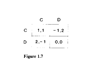
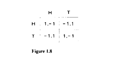
The set of equilibria of a finitely repeated game can be very different from that of the corresponding infinitely repeated game, because the scheme of self-reinforcing rewards and punishments used in the folk theorem can unravel backward from the terminal date. The classic example of this is the repeated prisoner’s dilemma. As observed in chapter 4, with a fixed finite horizon “always defect” is the only subgame-perfect-equilibrium outcome. In fact, with a bit more work one can show this is the only Nash outcome:

Fix a Nash equilibrium $\sigma^$. Both players must cheat in the last period, $T$, for any history $h^T$ that has positive probability under $\sigma^$, since doing so increases their period- $T$ payoff and since there are no future periods in which they might be punished. Next, we claim that both players must defect in period $T-1$ for any history $h^{T-1}$ with positive probability: We have already established that both players will chcat in the last period along the equilibrium path, so in particular if player $i$ conforms to the equilibrium strategy in period $T-1$ his opponent will defect in the last period, and hence player $i$ has no incentive not to defect in period $T-1$. An induction argument completes the proof. This conclusion, though not pathological, relies on the fact that the static equilibrium gives the players exactly their minmax values, as the following theorem shows.

经济代写|博弈论代写Game Theory代考|Repeated Games with Long-Run and Short-Run Players

The first variant we will consider supposes that some of the players are long-run players, as in standard repeated games, while the roles corresponding to other “players” are filled by a sequence of short-run players, each of whom plays only once.
Example 5.1
Suppose that a single long-run firm faces a sequence of short-run consumers, each of whom plays only once but is informed of all previous play when choosing his actions. Each period, the consumer moves first, and chooses whether or not to purchase a good from the firm. If the consumer does not purchase, then both players receive a payoff of 0 . If the consumer decides to purchase, then the firm must decide whether to produce high or low quality. If it produces high quality, both players have a payoff of 1 ; if it produces low quality, the firm’s payoff is 2 and the consumer’s payoff is

This game is a simplified version of those considered by Dybvig and Spatt (1980), Klein and Lefler (1981), and Shapiro (1982). ${ }^{12}$ Simon (1951)

and Kreps (1986) use a similar game to analyze the employment relationship, and to argue that one reason for the existence of “firms” is precisely to provide a long-run player who can be induced to be trustworthy by the prospect of future rewards and punishments.

The following strategies are a subgame-perfect equilibrium of this game when the firm is sufficiently patient: The firm starts out producing high yuality cvery time a consumer purchases, and continues to do so as long as it has never produced low quality in the past. If ever the firm produces low quality, it produces low quality at every subsequent opportunity. The consumers start out purchasing the good from the firm, and continue to do so so long as the firm has never produced low quality. If ever the firm produces low quality, then no consumer ever purchases again. The consumer’s strategies are optimal because each consumer cares only about that period’s payoff, and thus should buy if and only if that period’s quality is expected to be high. The firm does incur a short-run cost by producing high quality. but when the firm is patient this cost is offset by the fear that producing low quality will drive away future consumers. Note that this equilibrium suggests why consumers may prefer to deal with a firm that is expected to remain in business for a while, as opposed to a “fly-by-night” firm for whom long-run considerations are unimportant.

博弈论代考

经济代写|博弈论代写Game Theory代考|Finitely Repeated Games

这些游戏代表了一个固定已知视界$T$的情况。每个$l=0,1, \ldots, T$上的策略空间如上所述;效用通常被认为是每期收益的时间平均值。允许接近1的贴现因子$\delta$不会改变我们提出的结论。

有限重复博弈的平衡集可能与相应的无限重复博弈的平衡集非常不同，因为民间定理中使用的自我强化奖惩方案可以从结束日期向后分解。典型的例子是重复囚徒困境。正如在第4章中所观察到的，在固定的有限视界下，“总是缺陷”是唯一的子博弈-完美均衡结果。事实上，只要多做一点工作，就可以证明这是唯一的纳什结果:

修复纳什均衡$\sigma^$。两个玩家都必须在最后一个时期$T$，对于任何历史$h^T$，在$\sigma^$下有正概率，因为这样做增加了他们的时期- $T$收益，因为没有未来的时期，他们可能会受到惩罚。接下来，我们声称对于任何历史$h^{T-1}$，两个参与者都必须在时期$T-1$以正概率叛变:我们已经确定两个参与者都将在最后一个时期沿着均衡路径进行投机，所以特别是如果参与者$i$在时期$T-1$符合均衡策略，他的对手将在最后一个时期叛变，因此参与者$i$没有动机不在$T-1$时期叛变。一个归纳论证完成了这个证明。这一结论虽然不是病态的，但却是基于静态平衡能够提供给玩家最大最小值这一事实，如下面的定理所示。

经济代写|博弈论代写Game Theory代考|Repeated Games with Long-Run and Short-Run Players

我们将考虑的第一种变体假设一些玩家是长期玩家，就像在标准的重复游戏中一样，而与其他“玩家”对应的角色则由一系列短期玩家填补，每个玩家只玩一次。
例5.1
假设一个长期企业面对一系列短期消费者，每个消费者只玩一次游戏，但在选择行动时被告知之前的所有游戏。每个时期，消费者首先行动，选择是否从公司购买商品。如果消费者不购买，那么双方的收益都是0。如果消费者决定购买，那么企业必须决定生产高质量还是低质量的产品。如果产出高质量的产品，双方的收益都是1;如果生产低质量产品，公司的收益是2，消费者的收益是

这个游戏是Dybvig和Spatt (1980)， Klein和Lefler(1981)以及Shapiro(1982)所考虑的游戏的简化版本。${ }^{12}$西蒙(1951)

和Kreps(1986)用一个类似的游戏来分析雇佣关系，并认为“公司”存在的一个原因正是提供一个长期的参与者，他们可以被未来的奖励和惩罚的前景诱导为值得信赖的。

当公司有足够的耐心时，以下策略是该博弈的子博弈完美均衡:每次消费者购买时，公司都会开始生产高质量的产品，并且只要它过去从未生产过低质量的产品，就会继续这样做。如果一家公司曾经生产过低质量的产品，那么它在随后的每一次机会中都会生产低质量的产品。消费者开始从公司购买商品，只要公司不生产低质量的产品，消费者就会继续购买。如果企业生产的产品质量很差，那么消费者就不会再购买。消费者的策略是最优的，因为每个消费者只关心那段时间的收益，因此当且仅当那段时间的质量预期很高时，他们才会购买。这家公司生产高质量的产品确实产生了短期成本。但是，如果企业有耐心，这种成本就会被担心生产低质量产品会赶走未来的消费者所抵消。值得注意的是，这种平衡表明了为什么消费者可能更愿意与那些有望维持一段时间的公司打交道，而不是那些对长期考虑不重要的“不可靠”的公司。

经济代写|博弈论代写Game Theory代考请认准statistics-lab™

统计代写请认准statistics-lab™. statistics-lab™为您的留学生涯保驾护航。

金融工程代写

金融工程是使用数学技术来解决金融问题。金融工程使用计算机科学、统计学、经济学和应用数学领域的工具和知识来解决当前的金融问题，以及设计新的和创新的金融产品。

非参数统计代写

非参数统计指的是一种统计方法，其中不假设数据来自于由少数参数决定的规定模型；这种模型的例子包括正态分布模型和线性回归模型。

广义线性模型代考

广义线性模型（GLM）归属统计学领域，是一种应用灵活的线性回归模型。该模型允许因变量的偏差分布有除了正态分布之外的其它分布。

术语广义线性模型（GLM）通常是指给定连续和/或分类预测因素的连续响应变量的常规线性回归模型。它包括多元线性回归，以及方差分析和方差分析（仅含固定效应）。

有限元方法代写

有限元方法（FEM）是一种流行的方法，用于数值解决工程和数学建模中出现的微分方程。典型的问题领域包括结构分析、传热、流体流动、质量运输和电磁势等传统领域。

有限元是一种通用的数值方法，用于解决两个或三个空间变量的偏微分方程（即一些边界值问题）。为了解决一个问题，有限元将一个大系统细分为更小、更简单的部分，称为有限元。这是通过在空间维度上的特定空间离散化来实现的，它是通过构建对象的网格来实现的：用于求解的数值域，它有有限数量的点。边界值问题的有限元方法表述最终导致一个代数方程组。该方法在域上对未知函数进行逼近。[1] 然后将模拟这些有限元的简单方程组合成一个更大的方程系统，以模拟整个问题。然后，有限元通过变化微积分使相关的误差函数最小化来逼近一个解决方案。

tatistics-lab作为专业的留学生服务机构，多年来已为美国、英国、加拿大、澳洲等留学热门地的学生提供专业的学术服务，包括但不限于Essay代写，Assignment代写，Dissertation代写，Report代写，小组作业代写，Proposal代写，Paper代写，Presentation代写，计算机作业代写，论文修改和润色，网课代做，exam代考等等。写作范围涵盖高中，本科，研究生等海外留学全阶段，辐射金融，经济学，会计学，审计学，管理学等全球99%专业科目。写作团队既有专业英语母语作者，也有海外名校硕博留学生，每位写作老师都拥有过硬的语言能力，专业的学科背景和学术写作经验。我们承诺100%原创，100%专业，100%准时，100%满意。

随机分析代写

随机微积分是数学的一个分支，对随机过程进行操作。它允许为随机过程的积分定义一个关于随机过程的一致的积分理论。这个领域是由日本数学家伊藤清在第二次世界大战期间创建并开始的。

时间序列分析代写

随机过程，是依赖于参数的一组随机变量的全体，参数通常是时间。随机变量是随机现象的数量表现，其时间序列是一组按照时间发生先后顺序进行排列的数据点序列。通常一组时间序列的时间间隔为一恒定值（如1秒，5分钟，12小时，7天，1年），因此时间序列可以作为离散时间数据进行分析处理。研究时间序列数据的意义在于现实中，往往需要研究某个事物其随时间发展变化的规律。这就需要通过研究该事物过去发展的历史记录，以得到其自身发展的规律。

回归分析代写

多元回归分析渐进（Multiple Regression Analysis Asymptotics）属于计量经济学领域，主要是一种数学上的统计分析方法，可以分析复杂情况下各影响因素的数学关系，在自然科学、社会和经济学等多个领域内应用广泛。

MATLAB代写

MATLAB 是一种用于技术计算的高性能语言。它将计算、可视化和编程集成在一个易于使用的环境中，其中问题和解决方案以熟悉的数学符号表示。典型用途包括：数学和计算算法开发建模、仿真和原型制作数据分析、探索和可视化科学和工程图形应用程序开发，包括图形用户界面构建MATLAB 是一个交互式系统，其基本数据元素是一个不需要维度的数组。这使您可以解决许多技术计算问题，尤其是那些具有矩阵和向量公式的问题，而只需用 C 或 Fortran 等标量非交互式语言编写程序所需的时间的一小部分。MATLAB 名称代表矩阵实验室。MATLAB 最初的编写目的是提供对由 LINPACK 和 EISPACK 项目开发的矩阵软件的轻松访问，这两个项目共同代表了矩阵计算软件的最新技术。MATLAB 经过多年的发展，得到了许多用户的投入。在大学环境中，它是数学、工程和科学入门和高级课程的标准教学工具。在工业领域，MATLAB 是高效研究、开发和分析的首选工具。MATLAB 具有一系列称为工具箱的特定于应用程序的解决方案。对于大多数 MATLAB 用户来说非常重要，工具箱允许您学习和应用专业技术。工具箱是 MATLAB 函数（M 文件）的综合集合，可扩展 MATLAB 环境以解决特定类别的问题。可用工具箱的领域包括信号处理、控制系统、神经网络、模糊逻辑、小波、仿真等。

R语言代写	问卷设计与分析代写
PYTHON代写	回归分析与线性模型代写
MATLAB代写	方差分析与试验设计代写
STATA代写	机器学习/统计学习代写
SPSS代写	计量经济学代写
EVIEWS代写	时间序列分析代写
EXCEL代写	深度学习代写
SQL代写	各种数据建模与可视化代写

经济代写|博弈论代写Game Theory代考|Preemption Games

Posted on 2023年7月10日2023年7月10日 by statistics-lab

经济代写|博弈论代写Game Theory代考|Preemption Games

Preemption games are a rough opposite to the war of attrition, with $L(\hat{t})>F(\hat{t})$ for some range of times $\hat{t}$. Here the specification of the payoff to simultaneous stopping, $B(\cdot)$, is more important than in the war of attrition, as if $L$ exceeds $F$ we might expect both players to stop simultaneously. One example of a preemption game is the decision of whether and when to build a new plant or adopt a new innovation when the market is big enough to support only one such addition (Reinganum 1981a,b; Fudenberg and Tirole 1985). In this case $B(t)$ is often less than $F(t)$, as it cian be better to let an opponent have a monopoly than to incur duopoly losses.
()ne very stylized preemption game is “grab the dollar.” In this stationary game, time is discrete $(t=0,1, \ldots)$ and there is a dollar on the tablc, which either or both of the players can try to grab. If only one player grabs, that player receives 1 and the other 0 ; if both try to grab at once, the dollar is destroyed and both pay a fine of 1 ; if neither player grabs, the dollar remains on the table. The players use the common discount factor $\delta$, so that $l(t)=\delta^{\prime}, F(t)=0$, and $B(t)=-\delta^t$ for all $t$. Like the war of attrition, this game has asymmetric equilibria, where one player “wins” with probability 1. and also a symmetric mixed-strategy equilibrium, where each player grabs the dollar with probability $p^=\frac{1}{2}$ in cach period. (It is easy to check that this yields a symmetric equilibrium; to see that it is the only one, note that each player must be indifferent between stopping-i.e., grabbing-at date $t$, which yields payoff $\delta^{\prime}\left(\left(1-p^(t)\right)-p^(t)\right)$ if the other has not stopped before date $t$ and 0 otherwise, and never stopping, which yields payoff 0 , so that $p^(t)$ must equal $\frac{1}{2}$ for all $t$.) The payoffs in the symmetric cquilibrium are $(0,0)$, and the distribution over outcomes is that the probability that player 1 alone stops first at $t$, the probability that player 2 alone stops first at $t$, and the probability that both players stop simultaneously at $l$ are all equal to $\left({ }_4^1\right)^{t+1}$. Note that these probabilities are independent of the per-period discount factor, $\delta$, and thus of the period length, $\Lambda$, in contrast to the war of attrition, where the probabilities were proportional to the period length. This makes finding a continuous-time representation of this game more difficult.

经济代写|博弈论代写Game Theory代考|Iterated Conditional Dominance and the Rubinstein Bargaining Game

The last two sections presented several examples of infinite-horizon games with unique equilibria. The uniqueness arguments there can be strengthened, in that these games have a unique profile that satisfies a weaker concept than subgame perfection.

Definition 4.2 In a multi-stage game with observed actions, action $a_i^t$ is conditionally dominated at stage $t$ given history $h^t$ if, in the subgame beginning at $h^{\prime}$, every strategy for player $i$ that assigns positive probability to $a_i^{\prime}$ is strictly dominated. Iterated conditional dominance is the process that, at each round, deletes every conditionally dominated action in every subgame, given the opponents’ strategies that have survived the previous rounds.

It is easy to check that itcrated conditional dominance coincides with subgame perfection in finite games of perfect information. In these games it also coincides with Pearce’s (1984) extensive-form rationalizability. In general multi-stage games, any action ruled out by iterated conditional dominance is also ruled out by extensive-form rationalizability, but the cxact relationship between the two concepts has not been determined.
In a game of imperfect information, iterated conditional dominance can be weaker than subgame perfection, as it does not assume that players forecast that an equilibrium will occur in every subgame. To illustrate this point, consider a one-stage, simultaneous-move game. Then iterated conditional dominance coincides with iterated strict dominance, subgame perfection coincides with Nash equilibrium, and iterated strict dominance is in general weaker than Nash equilibrium.

博弈论代考

经济代写|博弈论代写Game Theory代考|Preemption Games

抢占式游戏与消耗战截然相反 $L(\hat{t})>F(\hat{t})$ 在一段时间内 $\hat{t}$．这里是同时停止的收益说明， $B(\cdot)$，比在消耗战中更重要，仿佛 $L$ 超过 $F$ 我们可能会期望两个玩家同时停下来。抢占游戏的一个例子是，当市场足够大，只能支持一种新产品时，决定是否以及何时建立新工厂或采用新创新(Reinganum 1981a,b;Fudenberg and Tirole 1985)。在这种情况下 $B(t)$ 通常小于 $F(t)$因为让对手垄断总比造成双寡头垄断的损失要好。
一个非常程式化的抢占游戏是“抢钱”。在这个静止博弈中，时间是离散的 $(t=0,1, \ldots)$ 桌上有一美元，任何一方或双方都可以试着去抢。如果只有一个玩家抓到了，那么这个玩家得到1，而另一个玩家得到0;如果双方都试图同时抢钱，美元就会被销毁，双方都要支付1美元的罚款;如果双方都没有抢到，那美元就留在桌上。玩家使用常见的折现系数 $\delta$，所以 $l(t)=\delta^{\prime}, F(t)=0$，和 $B(t)=-\delta^t$ 对所有人 $t$．与消耗战一样，这款游戏也具有非对称均衡，即一方玩家以1的概率“获胜”。还有一个对称的混合策略均衡，每个玩家都有概率地获得1美元 $p^=\frac{1}{2}$ 在每个时期。(很容易检验这是否产生对称平衡;要看到它是唯一的，注意每个玩家必须在停止之间无动于衷。，抓——在日期 $t$，产生收益 $\delta^{\prime}\left(\left(1-p^(t)\right)-p^(t)\right)$ 如果对方在约会前没有停止 $t$ 否则为0，永不停止，收益为0，所以 $p^(t)$ 必须相等 $\frac{1}{2}$ 对所有人 $t$)对称均衡的收益是 $(0,0)$结果的分布是参与人1首先停在 $t$，参与人2首先停在。的概率 $t$，以及两个玩家同时停在 $l$ 都等于 $\left({ }_4^1\right)^{t+1}$．请注意，这些概率与每周期的折现系数无关， $\delta$，因此周期长度， $\Lambda$而在消耗战中，概率与时间长短成正比。这使得寻找游戏的连续时间表现变得更加困难。

经济代写|博弈论代写Game Theory代考|Iterated Conditional Dominance and the Rubinstein Bargaining Game

最后两节介绍了具有独特均衡的无限视界博弈的几个例子。这里的独特性论点可以得到加强，因为这些游戏具有独特的特征，能够满足比子游戏完美性更弱的概念。

定义4.2在一个具有观察到的动作的多阶段博弈中，如果在从$h^{\prime}$开始的子博弈中，玩家$i$分配给$a_i^{\prime}$正概率的每个策略都是严格劣势的，那么在给定历史的$t$阶段，动作$a_i^t$是有条件劣势的$h^t$。迭代条件优势是指在每个回合中，根据对手在前几轮中幸存下来的策略，删除每个子游戏中的每个条件优势行动的过程。

在完全信息有限博弈中，迭代条件优势与子博弈完美性是一致的。在这些游戏中，它也与Pearce(1984)的广泛形式合理化相吻合。在一般的多阶段游戏中，任何被迭代条件支配所排除的行动也会被广泛形式的合理性所排除，但这两个概念之间的确切关系尚未确定。
在信息不完全的博弈中，迭代条件支配可能比子博弈的完美性更弱，因为它不假设玩家预测每个子博弈都会出现均衡。为了说明这一点，我们考虑一个单阶段同步移动的游戏。然后迭代条件优势与迭代严格优势重合，子博弈完美性与纳什均衡重合，迭代严格优势一般弱于纳什均衡。

统计代写请认准statistics-lab™. statistics-lab™为您的留学生涯保驾护航。

金融工程代写

非参数统计代写

非参数统计指的是一种统计方法，其中不假设数据来自于由少数参数决定的规定模型；这种模型的例子包括正态分布模型和线性回归模型。

广义线性模型代考

广义线性模型（GLM）归属统计学领域，是一种应用灵活的线性回归模型。该模型允许因变量的偏差分布有除了正态分布之外的其它分布。

有限元方法代写

随机分析代写

时间序列分析代写

回归分析代写

MATLAB代写

R语言代写	问卷设计与分析代写
PYTHON代写	回归分析与线性模型代写
MATLAB代写	方差分析与试验设计代写
STATA代写	机器学习/统计学习代写
SPSS代写	计量经济学代写
EVIEWS代写	时间序列分析代写
EXCEL代写	深度学习代写
SQL代写	各种数据建模与可视化代写

经济代写|博弈论代写Game Theory代考|Iterated Strict Dominance and Nash Equilibrium

Posted on 2023年7月10日2023年7月10日 by statistics-lab

经济代写|博弈论代写Game Theory代考|Iterated Strict Dominance and Nash Equilibrium

If the extensive form is finite, so is the corresponding strategic form, and the Nash existence theorem yields the existence of a mixed-strategy equilibrium. The notion of iterated strict dominance extends to extensiveform games as well; however, as we mentioned above, this concept turns out to have little force in most extensive forms. The point is that a player cannot strictly prefer one action over another at an information set that is not reached given his opponents’ play.

Consider figure 3.14. Here, player 2’s strategy $\mathrm{R}$ is not strictly dominated, as it is as good as $\mathrm{L}$ when player 1 plays $\mathrm{U}$. Morcover, this fact is not “pathological.” It obtains for all strategic forms whose payoffs are derived from an extensive form with the tree on the left-hand side of the figure. That is, for any assignment of payoffs to the terminal nodes of the tree, the payoffs to (U, L) and (U, R) must be the same, as both strategy profiles lead to the same terminal node. This shows that the set of strategic-form payoffs of a fixed game tree is of lower dimension than the set of all payoffs of the corresponding strategic form, so theorems based on generic strategic-form payoffs (see chapter 12) do not apply. In particular, there can be an even number of Nash equilibria for an open set of extensive-form payoffs. The game illustrated in figure 3.14 has two Nash equilibria, (U, R) and (D, L), and this number is not changed if the extensive-form payoffs are slightly perturbed. The one case where the odd-number theorem of chapter 12 applies is to a simultaneous-move game such as that of figure 3.4 ; in such a game, each terminal node corresponds to a unique strategy profile. Put differently: In simultaneous-move games, every strategy profile reaches every information set, and so no player’s strategy can involve a choice that is not implemented given his opponents’ play.

Recall that a game of perfect information has all its information sets as singletons, as in the games illustrated in figures 3.3 and 3.14 .

经济代写|博弈论代写Game Theory代考|Backward Induction and Subgame Perfection

As we have seen, the strategic form can be used to represent arbitrarily complex extensive-form games, with the strategies of the strategic form being complete contingent plans of action in the extensive form. Thus, the concept of Nash equilibrium can be applied to all games, not only to games where players choose their actions simultancously. However, many game theorists doubt that Nash equilibrium is the right solution concept for general games. In this section we will present a first look at “equilibrium refinements,” which are designed to separate the “reasonable” Nash equilibria from the “unreasonable” ones. In particular, we will discuss the ideas of backward induction and “subgame perfection.” Chapters 4, 5 and 13 apply these ideas to some classes of games of interest to economists.

Selten (1965) was the first to argue that in general extensive games some of the Nash equilibria are “more reasonable” than others. He began with the example illustrated here in figure 3.14. This is a finite game of perfect information, and the backward-induction solution (that is, the one obtained using Kuhn’s algorithm) is that player 2 should play $\mathrm{L}$ if his information set is reached, and so player 1 should play D. Inspection of the strategic form corresponding to this game shows that there is another Nash equilibrium, where player 1 plays $\mathrm{U}$ and player 2 plays $\mathrm{R}$. The profile $(\mathrm{U}, \mathrm{R})$ is a Nash equilibrium because, given that player 1 plays U, player 2’s information set is not reached, and player 2 loses nothing by playing R. But Selten argued, and we agree, that this equilibrium is suspect. After all, if player 2 ‘s information set is reached, then, as long as player 2 is convinced that his payoffs are as specified in the figure, player 2 should play $\mathbf{L}$. And if we were player 2 , this is how we would play. Moreover, if we were player 1 , we would expect player 2 to play $\mathbf{L}$, and so we would play $\mathrm{D}$.

In the now-familiar language, the equilibrium (U,R) is not “credible,” because it relies on an “empty threat” by player 2 to play $R$. The threat is “empty” because player 2 would never wish to carry it out.

博弈论代考

经济代写|博弈论代写Game Theory代考|Iterated Strict Dominance and Nash Equilibrium

如果扩展形式是有限的，那么相应的策略形式也是有限的，纳什存在性定理给出了混合策略均衡的存在性。迭代严格支配的概念也延伸到广泛形式的游戏中;然而，正如我们上面提到的，这个概念在大多数广泛的形式中几乎没有力量。关键在于，玩家不能严格地选择一种行动，而不是另一种行动。

考虑图3.14。在这里，参与人2的策略$\mathrm{R}$不是严格劣势，因为当参与人1的策略$\mathrm{U}$时，它和$\mathrm{L}$一样好。此外，这个事实并不是“病态的”。它适用于所有战略形式，其收益由图左侧的树状图导出。也就是说，对于树的终端节点的任何收益分配，(U, L)和(U, R)的收益必须是相同的，因为两种策略profile都指向相同的终端节点。这表明固定博弈树的策略形式收益集合比相应策略形式的所有收益集合的维数更低，因此基于一般策略形式收益的定理(见第12章)不适用。特别地，对于一个开放的广泛形式收益集，可以有偶数个纳什均衡。图3.14所示的博弈有两个纳什均衡(U, R)和(D, L)，如果泛化形式的收益受到轻微干扰，这个数字不会改变。第12章的奇数定理适用于图3.4这样的同时移动博弈;在这样的博弈中，每个终端节点对应一个唯一的策略配置文件。换句话说:在同步移动游戏中，每个策略配置文件都涉及到每个信息集，所以没有玩家的策略可以包含不考虑对手玩法的选择。

回想一下，一个完全信息博弈的所有信息集都是单信息，如图3.3和3.14所示。

经济代写|博弈论代写Game Theory代考|Backward Induction and Subgame Perfection

正如我们所看到的，战略形式可以用来表示任意复杂的广泛形式博弈，战略形式的策略是广泛形式中完整的偶然行动计划。因此，纳什均衡的概念可以应用于所有游戏，而不仅仅是玩家同时选择行动的游戏。然而，许多博弈论家怀疑纳什均衡是否是一般博弈的正确解概念。在本节中，我们将首先介绍“均衡优化”，它旨在将“合理的”纳什均衡与“不合理的”纳什均衡区分开来。特别地，我们将讨论逆向归纳法和“子博弈完善”的思想。第4章、第5章和第13章将这些思想应用于经济学家感兴趣的一些游戏类。

Selten(1965)是第一个提出在一般广泛博弈中，某些纳什均衡比其他均衡“更合理”的人。他从图3.14所示的例子开始。这是一个完全信息的有限博弈，逆向归纳解(即使用库恩算法得到的解)是，如果达到参与人2的信息集，参与人2应该选择$\ mathm {L}$，因此参与人1应该选择d。检查该博弈对应的策略形式表明，存在另一个纳什均衡，其中参与人1选择$\ mathm {U}$，参与人2选择$\ mathm {R}$。配置文件$(\ mathm {U}， \ mathm {R})$是纳什均衡，因为假设参与人1选择U，参与人2的信息集没有达到，参与人2选择R不会损失任何东西。但塞尔滕认为，我们同意，这个均衡是可疑的。毕竟，如果达到参与人2的信息集，那么，只要参与人2确信他的收益如图中所示，参与人2就应该选择$\mathbf{L}$。如果我们是参与人2，我们会这样玩。此外，如果我们是参与人1，我们会期望参与人2玩$\mathbf{L}$，所以我们会玩$\mathbf{D}$。

用现在熟悉的语言来说，均衡(U,R)不是“可信的”，因为它依赖于玩家2的“空威胁”来玩R。威胁是“空的”，因为玩家2永远不会想要执行它。

统计代写请认准statistics-lab™. statistics-lab™为您的留学生涯保驾护航。

金融工程代写

非参数统计代写

非参数统计指的是一种统计方法，其中不假设数据来自于由少数参数决定的规定模型；这种模型的例子包括正态分布模型和线性回归模型。

广义线性模型代考

广义线性模型（GLM）归属统计学领域，是一种应用灵活的线性回归模型。该模型允许因变量的偏差分布有除了正态分布之外的其它分布。

有限元方法代写

随机分析代写

时间序列分析代写

回归分析代写

MATLAB代写

R语言代写	问卷设计与分析代写
PYTHON代写	回归分析与线性模型代写
MATLAB代写	方差分析与试验设计代写
STATA代写	机器学习/统计学习代写
SPSS代写	计量经济学代写
EVIEWS代写	时间序列分析代写
EXCEL代写	深度学习代写
SQL代写	各种数据建模与可视化代写

经济代写|博弈论代写Game Theory代考|Backward Induction and Subgame Perfection

Posted on 2023年6月26日2023年6月26日 by statistics-lab

经济代写|博弈论代写Game Theory代考|Backward Induction and Subgame Perfection

In the Stackelberg game, it was easy to see how player 2 “ought” to play, because once $q_1$ was fixed player 2 faced a simple decision problem. This allowed us to solve for player 2 ‘s optimal second-stage choice for each $q_1$ and then work backward to find the optimal choice for player 1. This algorithm can be extended to other games where only one player moves at each stage. We say that a multi-stage game has perfect information if, for every stage $k$ and history $h^k$, exactly one player has a nontrivial choice set a choice set with more than one element and all the others have the one-element choice set “do nothing.” A simple example of such a game has player 1 moving in stages $0,2,4$, etc. and player 2 moving in stages $1,3,5$, and so on. More generally, some players could move several times in a row, and which player gets to move in stage $k$ could depend on the previous history. The key thing is that only one player moves at each stage $k$. Since we have assumed that each player knows the past choices of all rivals, this implies that the single player on move at $k$ is “perfectly informed” of all aspects of the game except those which will occur in the future.

Backward induction can be applied to any finite game of perfect information, where finite means that the number of stages is finite and the number of feasible actions at any stage is finite, too. The algorithm begins by determining the optimal choices in the final stage $K$ for each history $h^k$ that is, the action for the player on move, given history $h^\kappa$, that maximizes that player’s payoff conditional on $h^K$ being reached. (There may be more than one maximizing choice; in this case backward induction allows the player to choose any of the maximizers.) Then we work back to stage $K-1$, and determine the optimal action for the player on move there, given that the player on move at stage $K$ with history $h^K$ will play the action we determined previously. The algorithm proceeds to “roll back,” just as in solving decision problems, until the initial stage is reached. At this point we have constructed a strategy profile, and it is easy to verify that this maximizes that player’s payoff conditional on $h^{\mathrm{N}}$ being reached. (There may be more than one maximizing choice; in this case backward induction allows the player to choose any of the maximizers.) Then we work back to stage $K-1$, and determine the optimal action for the player on move there, given that the player on move at stage $K$ with history $h^K$ will play the action we determined previously. The algorithm proceeds to “roll back,” just as in solving decision problems, until the initial stage is reached. At this point we have constructed a strategy profile, and it is easy to verify that this profile is a Nash equilibrium. Moreover, it has the nice property that each player’s actions are optimal at every possible history.

The argument for the backward-induction solution in the two-stage Stackelberg game – that player 1 should be able to forecast player 2 ‘s second-stage play-strikes us as quite compelling. In a three-stage game,the argument is a bit more complex: The player on move at stage 0 must forecitst that the player on move at stage 1 will correctly forecast the play of the player on move at stage 2, which clearly is a more demanding hypothesis. And the arguments for backward induction in longer games require eorrespondingly more involved hypotheses. For this reason, backward-induction arguments may not be compelling in “long” games. For the moment, though, we will pass over the arguments against backward induction; section 3.6 discusses its limitations in more detail.

经济代写|博弈论代写Game Theory代考|The Value of Commitment and “Time Consistency”

One of the recurring themes in the analysis of dynamic games has been that in many situations players can benefit from the opportunity to make a binding commitment to play in a certain way. In a one-player game -i.e.. a decision problem – such commitments cannot be of value, as any payoff that a player could attain while playing according to the commitment could be attained by playing in exactly the same way without being committed to do so. With more than one player, though, commitments can be of value, since by committing himself to a given sequence of actions a player may be able to alter the play of his opponents. This “paradoxical” value of commitment is closely related to our observation in chapter 1 that a player can gain by reducing his action set or decreasing his payoff to some outcomes, provided that his opponents are aware of the change. Indeed, some forms of commitment can be represented in exactly this way.

The way to model the possibility of commitments (and related moves like “promises”) is to explicitly include them as actions the players can take. (Schelling (1960) was an early proponent of this view.) We have already seen one example of the value of commitment in our study of the Stackelberg game. which describes a situation where one firm (the “leader”) can commit itself to an output level that the follower is forced to take as given when making its own output decision. Under the typical assumption that each firm’s optimal reaction $r_i\left(q_j\right)$ is a decreasing function of its opponent’s output. the Stackelberg leader’s payoff is higher than in the “Cournot equilibrium” outcome where the two firms choose their output levels simultaneously.

In the Stackelberg example, commitment is achieved simply by moving earlier than the opponent. Although this corresponds to a different extensive form than the simultaneous moves of Cournot competition, the set of “physical actions” is in some sense the same. The search for a way to commit oneself can also lead to the use of actions that would not otherwise have been considered. Classic examples include a general burning his bridges behind him as a commitment not to retreat and Odysseus having himself lashed to the mast and ordering his sailors to plug their ears with wax as a commitment not to go to the Sirens” island. (Note that the natural way to model the Odysseus story is with two “players,” corresponding to ()dysseus before and Odysseus after he is exposed to the Sirens.) Both of these cases correspond to a “total commitment”: Once the bridge is burned, or Odysseus is lashed to the mast and the sailors’ ears are filled with wax, the cost of turning back or escaping from the mast is taken to be infinite. One can also consider partial commitments, which increase the cost of, c.g., turning back without making it infinite.

博弈论代考

经济代写|博弈论代写Game Theory代考|Backward Induction and Subgame Perfection

在Stackelberg博弈中，很容易看出玩家2“应该”怎么玩，因为一旦q_1$固定，玩家2将面临一个简单的决策问题。这让我们能够解出参与人2对于每个q_1$的第二阶段最优选择，然后反向找出参与人1的最优选择。这个算法可以扩展到其他在每个阶段只有一个玩家移动的游戏中。我们说一个多阶段博弈具有完美信息，如果对于每一个阶段$k$和历史$h^k$，只有一个参与者有一个非平凡的选择集一个包含多个元素的选择集而所有其他人都有一个“什么都不做”的单元素选择集举个简单的例子，玩家1在第0、2、4阶段移动，玩家2在第1、3、5阶段移动，以此类推。更一般地说，有些玩家可以连续移动几次，而哪个玩家可以在阶段k中移动可能取决于之前的历史。关键是每个阶段只有一个玩家移动。由于我们假设每个玩家都知道所有对手过去的选择，这意味着在k处移动的单个玩家“完全了解”游戏的所有方面，除了那些将在未来发生的事情。

逆向归纳法可以应用于任何具有完全信息的有限博弈，其中有限意味着阶段的数量是有限的，任何阶段的可行行动的数量也是有限的。算法首先确定最后阶段每个历史的最优选择，也就是说，给定历史，玩家移动时的行动，在达到h^K的条件下，最大化玩家的收益。(可能有不止一个最大化的选择;在这种情况下，逆向归纳允许玩家选择任何最大化者。)然后我们回到第K-1阶段，并确定在那里移动的玩家的最佳行动，因为在第K阶段具有历史$h^K$的移动玩家将采取我们之前确定的行动。算法继续“回滚”，就像解决决策问题一样，直到到达初始阶段。在这一点上，我们已经构建了一个策略概要，并且很容易验证这将最大化玩家的收益，条件是达到$h^{\ mathm {N}}$。(可能有不止一个最大化的选择;在这种情况下，逆向归纳允许玩家选择任何最大化者。)然后我们回到第K-1阶段，并确定在那里移动的玩家的最佳行动，因为在第K阶段具有历史$h^K$的移动玩家将采取我们之前确定的行动。算法继续“回滚”，就像解决决策问题一样，直到到达初始阶段。至此，我们已经构建了一个策略概要，并且很容易验证该概要是纳什均衡。此外，它还有一个很好的属性，即每个玩家的行动在每个可能的历史中都是最优的。

对于两阶段Stackelberg博弈的反向归纳解决方案，即参与人1应该能够预测参与人2在第二阶段的行为，我们认为这是非常有说服力的。在三阶段的游戏中，论证就复杂一些:在第0阶段移动的玩家必须预测在第1阶段移动的玩家能够正确预测在第2阶段移动的玩家的行为，这显然是一个要求更高的假设。在更长的博弈中，逆向归纳法的论证需要相应的更复杂的假设。出于这个原因，逆向归纳论证在“长”游戏中可能不那么有说服力。现在，我们先不讨论反对逆向归纳法的论点;第3.6节更详细地讨论了它的局限性。

经济代写|博弈论代写Game Theory代考|The Value of Commitment and “Time Consistency”

动态游戏分析中反复出现的一个主题是，在许多情况下，玩家可以从以某种方式进行游戏的约束性承诺中获益。在单人游戏中——例如……一个决策问题——这样的承诺不可能有价值，因为玩家在按照承诺进行游戏时可以获得的任何收益都可以在没有承诺的情况下以完全相同的方式进行游戏而获得。但是，如果有不止一个玩家，承诺就会有价值，因为通过承诺自己的特定行动序列，玩家可能会改变对手的玩法。这种承诺的“矛盾”价值与我们在第一章中观察到的密切相关，即玩家可以通过减少自己的行动集或减少某些结果的收益而获得收益，前提是他的对手意识到这种变化。的确，某些形式的承诺可以用这种方式来表示。

为承诺(以及“承诺”之类的相关动作)的可能性建模的方法是明确地将它们作为玩家可以采取的行动。(谢林(1960)是这一观点的早期支持者。)在研究Stackelberg博弈时，我们已经看到了承诺价值的一个例子。它描述了这样一种情况，即一个企业(“领导者”)可以承诺自己的产出水平，而追随者在做出自己的产出决策时被迫采取既定的产出水平。在典型的假设下，每个公司的最优反应$r_i\left(q_j\right)$是其对手产出的递减函数。在“古诺均衡”中，两家企业同时选择各自的产出水平。

在Stackelberg的例子中，承诺只是通过比对手更早行动来实现的。虽然这与古诺竞争的同时运动对应的是一种不同的广泛形式，但“身体动作”的集合在某种意义上是相同的。寻找一种方式来承诺自己也可以导致使用行动，否则不会被考虑。经典的例子包括一位将军烧毁了身后的桥梁，以保证不撤退;奥德修斯把自己绑在桅杆上，命令他的水手用蜡塞住耳朵，以保证不去塞壬的岛。(注意，奥德修斯故事的自然模型是两个“玩家”，对应于()之前的奥德修斯和之后的奥德修斯暴露在塞壬面前。)这两种情况都对应于一种“完全的承诺”:一旦桥被烧毁，或者奥德修斯被绑在桅杆上，水手们的耳朵被蜡填满，回头或逃离桅杆的代价被认为是无限的。我们也可以考虑部分承诺，这增加了成本，例如，回头而不使其无限。

统计代写请认准statistics-lab™. statistics-lab™为您的留学生涯保驾护航。

金融工程代写

非参数统计代写

非参数统计指的是一种统计方法，其中不假设数据来自于由少数参数决定的规定模型；这种模型的例子包括正态分布模型和线性回归模型。

广义线性模型代考

广义线性模型（GLM）归属统计学领域，是一种应用灵活的线性回归模型。该模型允许因变量的偏差分布有除了正态分布之外的其它分布。

有限元方法代写

随机分析代写

时间序列分析代写

回归分析代写

MATLAB代写

R语言代写	问卷设计与分析代写
PYTHON代写	回归分析与线性模型代写
MATLAB代写	方差分析与试验设计代写
STATA代写	机器学习/统计学习代写
SPSS代写	计量经济学代写
EVIEWS代写	时间序列分析代写
EXCEL代写	深度学习代写
SQL代写	各种数据建模与可视化代写

经济代写|博弈论代写Game Theory代考|An Application of Iterated Strict Dominance

Posted on 2023年6月26日2023年6月26日 by statistics-lab

经济代写|博弈论代写Game Theory代考|An Application of Iterated Strict Dominance

We now make stronger assumptions on the (infinite-action) Cournot model introduced in example 1.3: Suppose that $u_i$ is strictly concave in $q_i\left(\hat{i}^2 u_i / \hat{i} q_i^2<0\right)$, that the cross-partial derivative is negative $\left(\hat{C}^2 u_i / \hat{c} q_i \hat{\theta} q_j<\right.$ 0 . which is the case if $p^{\prime}<0$ and $p^{\prime \prime} \leq 0$ ), and that the reaction curves $r_1$ and $r_2$ (which are continuous and downward-sloping from the previous two assumptions) intersect only once at a point $N$, at which $r_1$ is strictly steeper than $r_2$. This situation is depicted in figure 2.1. (Note that $N$ is stable, in the terminology introduced in subsection 1.2.5.)

Let $q_1^m$ and $q_2^m$ denote the monopoly outputs: $q_1^m=r_1(0)$ and $q_2^m=r_2(0)$. The first round of deletion of strictly dominated strategies yields $S_i^1=$ $\left[0, q_i^m\right]$. The second round of deletion yields $S_i^2=\left[r_i\left(q_j^m\right), q_i^m\right] \equiv\left[q_i^2, q_i^m\right]$, as indicated in figure 2.1. Consider, for instance, firm 2. Knowing that firm 1 won’t pick output greater than $q_i^m$, choosing output $q_2$ under $r_2\left(q_1^m\right) \equiv q_2^2$ is strictly dominated by playing $q_2^2$ by strict concavity of firm 2 s payoff in its own output. And similarly for firm 1. The third round of deletion yields $S_i^3=\left[q_i^2, r_i\left(q_j^2\right)\right] \equiv\left[q_i^2, q_i^3\right]$, and so on. More generally, itcrated deletion yields a sequence of shrinking intervals around the outputs $\left(q_1^, q_2^\right)$ corresponding to the intersection $N$ of the reaction curves. For $n-2 k+1$,
$$
q_i^{2 k+1}=q_i^{2 k} \quad \text { and } \quad q_i^{2 k+1}=r_i\left(q_j^{2 k}\right) \text {; }
$$
for $n=2 k$,
$$
q_i^{2 k}=r_i\left(q_j^{2 k-1}\right) \quad \text { and } \quad q_i^{2 k}=\bar{q}_i^{2 k-1} \text {. }
$$
A diflerence between this process and the case of finite strategy spaces is that the process of deletion does not stop after a finite number of steps. Nevertheless, the process does converge, because the sequences $q_i^n$ and $q_i^n$ both converge to $q_i^$, so that the process of iterated deletion of strictly dominated strategies yields $N$ as the unique “reasonable” prediction. (Let $q_i^s \equiv \lim q_i^n \leq q_i^$ and $\bar{q}_i^{\infty} \equiv \lim q_i^n \geq q_i^$. From the definition of $q_i^n$ and $\bar{q}_i^n$ and by continuity of the reaction curves, one has $\bar{q}_i^{\infty}=r_i\left(q_j^{\infty}\right)$ and $q_j^{\infty}=$ $r_j\left(q_i^x\right)$. Hence, $\bar{q}_i^x=r_i\left(r_j\left(\bar{q}_i^x\right)\right)$, which is possibie only if $\bar{q}_i^{\infty}=q_i^$; and similarly for $q_i^x$.)
We conclude that this Cournot game is solvable by iterated strict dominance. This need not be the case for other specifications of the payoff functions; see exercise 2.4 .

经济代写|博弈论代写Game Theory代考|Rationalizability

The concept of rationalizability was introduced independently by Bernheim (1984) and Pearce (1984), and was used by Aumann (1987) and by Brandenberger and Dekel (1987) in their papers on the “Bayesian approach” to the choice of strategies.

Like iterated strict dominance, rationalizability derives restrictions on play from the assumptions that the payoffs and the “rationality” of the players are common knowledge. The starting point of iterated strict dominance is the observation that a rational player will never play a strictly dominated strategy. The starting point of rationalizability is the complementary question: What are all the strategies that a rational player could play? The answer is that a rational player will use only those strategies that are best responses to some beliefs he might have about the strategies of his opponents. Or, to use the contrapositive, a player cannot reasonably play a strategy that is not a best response to some beliefs about his opponents’ strategies. Moreover, since the player knows his opponents’ payoffs, and knows they are rational, he should not have arbitrary beliefs about their strategies. He should expect his opponents to use only strategies that are best responses to some beliefs that they might have. And these opponents’ beliefs, in turn, should also not be arbitrary, which leads to an infinite regress. In the two-player case, the infinite regress has the form “I’m playing strategy $\sigma_1$ because I think player 2 is using $\sigma_2$, which is a reasonable belief because I would play it if I were player 2 and I thought player 1 was using $\sigma_1^{\prime}$, which is a reasonable thing for player 2 to expect because $\sigma_1^{\prime}$ is a best response to $\sigma_2^{\prime}, \ldots$,

Formally, rationalizability is defined by the following iterative process.
Definition 2.3 Set $\tilde{\Sigma}i^o \equiv \Sigma_i$, and for each $i$ recursively define $$ \begin{aligned} & \tilde{\Sigma}_i^n=\left{\sigma_i \in \tilde{\Sigma}_i^{n-1} \mid \exists \sigma{-i} \in \underset{j \neq i}{\times} \text { convex hull }\left(\tilde{\Sigma}j^{n-1}\right)\right. \text { such that } \ & \left.u_i\left(\sigma_i, \sigma{-i}\right) \geq u_i\left(\sigma_i^{\prime}, \sigma_{-i}\right) \text { for all } \sigma_i^{\prime} \in \tilde{\Sigma}i^{n-1}\right} . \end{aligned} $$ The rationalizable strategies for player $i$ are $R_i=\bigcap{n=0}^{\infty} \tilde{\Sigma}_i^n$.

博弈论代考

经济代写|博弈论代写Game Theory代考|An Application of Iterated Strict Dominance

现在，我们对例1.3中介绍的(无限作用)古诺模型做出更强的假设:假设$u_i$在$q_i\left(\hat{i}^2 u_i / \hat{i} q_i^2<0\right)$中严格凹，交叉偏导数为负$\left(\hat{C}^2 u_i / \hat{c} q_i \hat{\theta} q_j<\right.$ 0。如果$p^{\prime}<0$和$p^{\prime \prime} \leq 0$)，反应曲线$r_1$和$r_2$(从前两个假设来看是连续的向下倾斜的)只在一点$N$相交一次，在这一点上$r_1$严格地比$r_2$陡峭。这种情况如图2.1所示。(请注意，按照第1.2.5小节介绍的术语，$N$是稳定的。)

让 $q_1^m$ 和 $q_2^m$ 表示垄断输出: $q_1^m=r_1(0)$ 和 $q_2^m=r_2(0)$．第一轮剔除严格劣势策略产生 $S_i^1=$ $\left[0, q_i^m\right]$．第二轮删除产生 $S_i^2=\left[r_i\left(q_j^m\right), q_i^m\right] \equiv\left[q_i^2, q_i^m\right]$，如图2.1所示。以公司2为例。知道公司1不会选择产出大于 $q_i^m$，选择输出 $q_2$ 在 $r_2\left(q_1^m\right) \equiv q_2^2$ 是严格以玩为主的吗 $q_2^2$ 通过公司2的收益在其自身产出中的严格凹性。公司1也是如此。第三轮删除产生 $S_i^3=\left[q_i^2, r_i\left(q_j^2\right)\right] \equiv\left[q_i^2, q_i^3\right]$等等。更一般地说，迭代删除会在输出周围产生一系列缩小间隔 $\left(q_1^, q_2^\right)$ 对应于交点 $N$ 反应曲线的。对于 $n-2 k+1$，
$$
q_i^{2 k+1}=q_i^{2 k} \quad \text { and } \quad q_i^{2 k+1}=r_i\left(q_j^{2 k}\right) \text {; }
$$
为了 $n=2 k$，
$$
q_i^{2 k}=r_i\left(q_j^{2 k-1}\right) \quad \text { and } \quad q_i^{2 k}=\bar{q}_i^{2 k-1} \text {. }
$$
这个过程与有限策略空间的不同之处在于，删除过程不会在有限的步骤之后停止。然而，这个过程是收敛的，因为序列 $q_i^n$ 和 $q_i^n$ 两者都收敛于 $q_i^$，使得严格劣势策略的迭代删除过程产生 $N$ 作为唯一的“合理”预测。(让 $q_i^s \equiv \lim q_i^n \leq q_i^$ 和 $\bar{q}_i^{\infty} \equiv \lim q_i^n \geq q_i^$．从 $q_i^n$ 和 $\bar{q}_i^n$ 根据反应曲线的连续性，我们有 $\bar{q}_i^{\infty}=r_i\left(q_j^{\infty}\right)$ 和 $q_j^{\infty}=$ $r_j\left(q_i^x\right)$．因此， $\bar{q}_i^x=r_i\left(r_j\left(\bar{q}_i^x\right)\right)$，这只有在 $\bar{q}_i^{\infty}=q_i^$；类似地 $q_i^x$.）
我们得出结论，该古诺博弈是可解的迭代严格优势。对于收益函数的其他规格则不必如此;参见练习2.4。

经济代写|博弈论代写Game Theory代考|Rationalizability

合理化的概念是由Bernheim(1984)和Pearce(1984)独立提出的，并被Aumann(1987)和Brandenberger和Dekel(1987)在他们关于策略选择的“贝叶斯方法”的论文中使用。

就像反复的严格支配一样，合理性基于玩家的收益和“合理性”是常识这一假设而产生对游戏的限制。迭代严格优势的出发点是观察到理性玩家永远不会采取严格劣势策略。合理性的出发点是一个互补的问题:一个理性的参与者可能采取的所有策略是什么?答案是，一个理性的参与者只会使用那些他对对手的策略所持有的信念的最佳对策。或者，用反命题来说，玩家不能合理地采取对对手策略的某些信念不是最佳反应的策略。此外，由于玩家知道对手的收益，知道他们是理性的，他不应该对他们的策略有武断的信念。他应该期望他的对手只使用对他们可能拥有的某些信念最好的回应策略。反过来，这些反对者的信念也不应该是武断的，这会导致无限的倒退。在两人博弈的情况下，无限回归的形式是”我选择策略$\sigma_1$因为我认为参与人2会选择$\sigma_2$，这是合理的假设因为如果我是参与人2我认为参与人1会选择$\sigma_1^{\prime}$，这是参与人2的合理预期因为$\sigma_1^{\prime}$是$\sigma_2^{\prime}, \ldots$的最佳对策，

形式上，合理性由以下迭代过程定义。
定义2.3设置$\tilde{\Sigma}i^o \equiv \Sigma_i$，并对每个$i$递归定义$$ \begin{aligned} & \tilde{\Sigma}i^n=\left{\sigma_i \in \tilde{\Sigma}_i^{n-1} \mid \exists \sigma{-i} \in \underset{j \neq i}{\times} \text { convex hull }\left(\tilde{\Sigma}j^{n-1}\right)\right. \text { such that } \ & \left.u_i\left(\sigma_i, \sigma{-i}\right) \geq u_i\left(\sigma_i^{\prime}, \sigma{-i}\right) \text { for all } \sigma_i^{\prime} \in \tilde{\Sigma}i^{n-1}\right} . \end{aligned} $$玩家$i$的合理策略为$R_i=\bigcap{n=0}^{\infty} \tilde{\Sigma}_i^n$。

统计代写请认准statistics-lab™. statistics-lab™为您的留学生涯保驾护航。

金融工程代写

非参数统计代写

非参数统计指的是一种统计方法，其中不假设数据来自于由少数参数决定的规定模型；这种模型的例子包括正态分布模型和线性回归模型。

广义线性模型代考

广义线性模型（GLM）归属统计学领域，是一种应用灵活的线性回归模型。该模型允许因变量的偏差分布有除了正态分布之外的其它分布。

有限元方法代写

随机分析代写

时间序列分析代写

回归分析代写

MATLAB代写

R语言代写	问卷设计与分析代写
PYTHON代写	回归分析与线性模型代写
MATLAB代写	方差分析与试验设计代写
STATA代写	机器学习/统计学习代写
SPSS代写	计量经济学代写
EVIEWS代写	时间序列分析代写
EXCEL代写	深度学习代写
SQL代写	各种数据建模与可视化代写

经济代写|博弈论代写Game Theory代考|Examples of Pure-Strategy Equilibria

Posted on 2023年6月26日2023年6月26日 by statistics-lab

经济代写|博弈论代写Game Theory代考|Examples of Pure-Strategy Equilibria

A simple example of nonexistence is “matching pennies” (figure 1.8). Players 1 and 2 simultaneously announce heads $(\mathrm{H})$ or tails $(\mathrm{T})$. If the announcements match, then player 1 gains a util and player 2 loses a util. If the announcements differ, it is player 2 who wins the util and player 1 who loses. If the predicted outcome is that the announcements will match, then player 2 has an incentive to deviate, while playcr 1 would prefer to deviate from any prediction in which announcements do not match. The only “stable” situation is one in which cach player randomizes between his two pure strategics, assigning equal probability to each. To see this, note that if player 2 randomizes $\frac{1}{2}-\frac{1}{2}$ between $\mathrm{H}$ and $\mathrm{T}$, player 1’s payoff is $\frac{1}{2} \cdot 1+\frac{1}{2} \cdot(-1)=0$ when playing $\mathrm{H}$ and $\frac{1}{2} \cdot(-1)+\frac{1}{2} \cdot 1=0$ when playing $T$. In this case player 1 is completely indifferent between his possible choices and is willing to randomize himself.

This raises the question of why a player should bother to play a mixed strategy when he knows that any of the pure strategies in its support would do equally well. In matching pennies, if player 1 knows that player 2 will randomize between $\mathrm{H}$ and $\mathrm{T}$ with equal probabilities, player 1 has expected value 0 from all possible choices. As far as his payoff goes, he could just as well play “heads” with certainty, but if this is anticipated by player 2 the equilibrium disintegrates. Subsection 1.2.5 mentions one defense of mixed strategies, which is that it represents a large population of players who use different pure strategies. If we insist that there is only one “player 1,” though, this interpretation does not apply. Harsanyi (1973a) offered the alternative defense that the “mixing” should be interpreted as the result of small, unobservable variations in a player’s payoffs. Thus, in our example, sometimes player 1 might prefer matching on $T$ to matching on $\mathbf{H}$, and conversely. Then, for each value of his payoff, player 1 would play a pure strategy. This “purification” of mixed-strategy equilibria is discussed in chapter 6 .

经济代写|博弈论代写Game Theory代考|Multiple Nash Equilibria, Focal Points, and Pareto Optimality

Many games have several Nash equilibria. When this is the case, the assumption that a Nash equilibrium is played relies on there being some mechanism or process that leads all the players to expect the same equilibrium.

One well-known example of a game with multiple equilibria is the “battle of the sexes,” illustrated by figure 1.10a. The story that goes with the name “battle of the sexes” is that the two players wish to go to an event together, but disagree about whether to go to a football game or the ballet. Each player gets a utility of 2 if both go to his or her preferred event, a utility of 1 if both go to the other’s preferred event, and 0 if the two are unable to agree and stay home or go out individually. Figure $1.10 \mathrm{~b}$ displays a closely related game that goes by the names of “chicken” and “hawk-dove.” (Chapter 4 discusses a related dynamic game that is also called “chicken.”) One version of the story here is that the two players meet at a one-lane bridge and each must choose whether to cross or to wait for the other. If both play T (for “tough”), they crash in the middle of the bridge and get -1 each; if both play W (for “weak”), they wait and get 0 ; if one player chooses $\mathrm{T}$ and the other chooses $\mathrm{W}$, then the tough player crosses first, receiving 2, and the weak one receives 1 . In the bridge-crossing story, the term “chicken” is used in the colloquial sense of “coward.” (Evolutionary biologists call this game “hawk-dove,” because they interpret strategy T as “hawk-like” and strategy W as “dove-like.”)

Though the different payoff matrices in figures $1.10 \mathrm{a}$ and $1.10 \mathrm{~b}$ describe different sorts of situations, the two games are very similar. Each of them has three equilibria: two in pure strategies, with payoffs $(2,1)$ and $(1,2)$, and

Building on this result, one can compute the optimal contract, i.e., the $w$ that maximizes the principal’s expected payorI
$$
r(1-x) \cdot w(1-x y)-h y=v(1-h / w)-w .
$$
The optimal wage is thus $w-\sqrt{h}$ (assuming $\sqrt{h} v>g$ ). Note that the principal would be better off if he could “commit” to an inspection level. To see this, consider the different game in which the principal plays first and chooses a probability $y$ of inspection, and the agent, after vbserving $y$, chooses whether to shirk. For a given $w(>g)$, the principal can choose $y=4 / u+c$, where $\varepsilon$ is positive and arbitrarily small. The agent then works with probability 1, and the principal has (approximately) payoff
$$
r-w \cdot h g(w>v(1-h ; w)-w \text {. }
$$
Technically, commitment eliminates the constraint $x w \geq h$, (i.e., that it is ex post worthwhile to inspect). (It is crucial that the principal is committed to inspecting with probability $y$. If the “toss of the coin” determining inspection is not public, the principal has an ex post incentive not to inspect, as he knows that the agent works.) This reasoning will become familiar in chapter 3 . See chapters 5 and 10 for discussions of how repeated play might make the commitment credible whereas it would not be if the game was played only once.

博弈论代考

经济代写|博弈论代写Game Theory代考|Examples of Pure-Strategy Equilibria

不存在的一个简单例子是“匹配便士”(图1.8)。玩家1和玩家2同时宣布正面$(\mathrm{H})$或反面$(\mathrm{T})$。如果公告匹配，则玩家1获得一个util，玩家2失去一个util。如果公告不同，则玩家2赢了，玩家1输了。如果预测结果是公告匹配，那么玩家2就有偏离的动机，而玩家1则更愿意偏离公告不匹配的预测。唯一“稳定”的情况是每个玩家随机选择自己的两种纯策略，并为每种策略分配相同的概率。要看到这一点，请注意，如果玩家2在$\mathrm{H}$和$\mathrm{T}$之间随机选择$\frac{1}{2}-\frac{1}{2}$，那么玩家1在使用$\mathrm{H}$时的收益是$\frac{1}{2} \cdot 1+\frac{1}{2} \cdot(-1)=0$，在使用$T$时的收益是$\frac{1}{2} \cdot(-1)+\frac{1}{2} \cdot 1=0$。在这种情况下，参与人1对可能的选择完全无所谓，他愿意随机选择自己。

这就提出了一个问题:当玩家知道任何纯策略的支持效果都一样好时，他为什么还要选择混合策略呢?在硬币匹配中，如果参与人1知道参与人2将以相同的概率在$\mathrm{H}$和$\mathrm{T}$之间随机抽取，那么参与人1在所有可能选择中的期望值为0。就他的收益而言，他也可以肯定地打出“正面”，但如果参与人2预料到这一点，那么均衡就会瓦解。第1.2.5小节提到了对混合策略的一种辩护，即混合策略代表了大量使用不同纯策略的玩家。如果我们坚持认为只有一个“玩家1”，那么这种解释就不适用了。Harsanyi (1973a)提出了另一种辩护，认为“混合”应该被解释为参与者收益中微小的、不可观察的变化的结果。因此，在我们的示例中，有时玩家1可能更喜欢在$T$上匹配而不是在$\mathbf{H}$上匹配，反之亦然。然后，对于每个收益值，参与人1将采取纯策略。混合策略均衡的这种“净化”将在第6章中讨论。

经济代写|博弈论代写Game Theory代考|Multiple Nash Equilibria, Focal Points, and Pareto Optimality

许多博弈都有几个纳什均衡。在这种情况下，纳什均衡的假设依赖于某种机制或过程使所有参与者期望相同的均衡。

“两性之战”是具有多重平衡的游戏的一个著名例子，如图1.10a所示。与“性别之战”同名的故事是，两个玩家希望一起去参加一个活动，但不同意是去看足球比赛还是看芭蕾舞。如果双方都选择自己喜欢的事件，每个参与人的效用为2，如果双方都选择对方喜欢的事件，效用为1，如果双方不能达成一致，各自待在家里或外出，效用为0。图$1.10 \mathrm{~b}$显示了一个密切相关的游戏，名为“鸡”和“鹰鸽”。(游戏邦注:第4章讨论的是一个相关的动态游戏，也被称为“chicken”)故事的一个版本是，两个玩家在单车道的桥上相遇，每个人都必须选择是过去还是等待另一个。如果两人都选择T(代表“强硬”)，他们就会在桥的中间坠毁，各得-1分;如果两人都玩W(代表“弱”)，他们等待并得到0;如果一个玩家选择$\mathrm{T}$，另一个玩家选择$\mathrm{W}$，那么强壮的玩家先传中，得2分，弱的玩家得1分。在过桥的故事中，“chicken”这个词的口语意思是“懦夫”。(进化生物学家称这种博弈为“鹰鸽”，因为他们将策略T解释为“鹰式”，将策略W解释为“鸽式”。)

虽然图$1.10 \mathrm{a}$和$1.10 \mathrm{~b}$中不同的收益矩阵描述了不同的情况，但这两个游戏非常相似。每个人都有三个均衡两个是纯策略，收益分别是$(2,1)$和$(1,2)$，还有

在此结果的基础上，可以计算出最优合约，即使本金预期支付ori最大化的$w$
$$
r(1-x) \cdot w(1-x y)-h y=v(1-h / w)-w .
$$
因此，最优工资是$w-\sqrt{h}$(假设$\sqrt{h} v>g$)。请注意，如果委托人能够“承诺”一个检查级别，他的境况会更好。要了解这一点，请考虑不同的博弈，其中委托人先玩并选择检查的概率$y$，代理在vbserving $y$之后选择是否逃避。对于给定的$w(>g)$，委托人可以选择$y=4 / u+c$，其中$\varepsilon$为正且任意小。然后，代理人以概率为1的方式工作，委托人获得(近似)收益
$$
r-w \cdot h g(w>v(1-h ; w)-w \text {. }
$$
从技术上讲，承诺消除了$x w \geq h$约束(即，事后值得检查)。(至关重要的是，委托人承诺以概率检查$y$。如果决定检查的“掷硬币”不是公开的，委托人就有事后不检查的动机，因为他知道代理人在工作。)这个推理在第三章中会变得很熟悉。在第5章和第10章中，我们讨论了重复游戏是如何让承诺变得可信的，而如果游戏只玩一次就不会如此。

统计代写请认准statistics-lab™. statistics-lab™为您的留学生涯保驾护航。

金融工程代写

非参数统计代写

非参数统计指的是一种统计方法，其中不假设数据来自于由少数参数决定的规定模型；这种模型的例子包括正态分布模型和线性回归模型。

广义线性模型代考

广义线性模型（GLM）归属统计学领域，是一种应用灵活的线性回归模型。该模型允许因变量的偏差分布有除了正态分布之外的其它分布。

有限元方法代写

随机分析代写

时间序列分析代写

回归分析代写

MATLAB代写

R语言代写	问卷设计与分析代写
PYTHON代写	回归分析与线性模型代写
MATLAB代写	方差分析与试验设计代写
STATA代写	机器学习/统计学习代写
SPSS代写	计量经济学代写
EVIEWS代写	时间序列分析代写
EXCEL代写	深度学习代写
SQL代写	各种数据建模与可视化代写

经济代写|博弈论代写Game Theory代考|PROBABILITY

Posted on 2023年6月7日2023年6月7日 by statistics-lab

经济代写|博弈论代写Game Theory代考|PROBABILITY

A coin toss produces a random event, where the outcome can be either “heads” or “tails.” For a “fair” coin, we assess that these outcomes are equally likely. Sometimes we use the phrase “fifty-fifty” to describe the prospects. In more formal terms, we would say that the probability of heads is $1 / 2$ and the probability of tails is $1 / 2$. Using the concept of probability, we have an organized and logical way of considering random events.

There are all sorts of situations that have random components. The weather is random, machines fail randomly, and sometimes people behave randomly. To study the random component, it is useful to consider a state space that describes all of the possible resolutions of the random forces. For example, if you are interested in a particular horse race, the state space may consist of all of the different orderings of the horses (ways in which they could finish in the race). If you are a poker player, the state space may comprise the different ways in which the cards can be dealt. If you like flipping coins, the state space is ${$ heads, tails $}$. Each of the states in the state space is assumed to describe an outcome that is mutually exclusive of what other states describe. Further, the states collectively exhaust all of the possibilities. In other words, one and only one state actually occurs.

To describe the relative likelihood of the different individual states, we can posit a probability distribution over the state space. For example, suppose the state space is ${A, B, C}$. Think of this as the possible outcomes of a horse race, where all you care about is which horse wins (horse $A$, horse $B$, or horse $C$ ). A probability distribution for this state space implies a function $p:{A, B, C} \rightarrow[0,1]$ from which we get three numbers, $p(A), p(B)$, and $p(C)$. The number $p(A)$ is the “probability that $A$ occurs,” $p(B)$ is the probability that $B$ occurs, and $p(C)$ is the probability that $C$ occurs. Each of these numbers is assumed to be between 0 and 1 (as you can see from the codomain designation of $p$ ) and the numbers sum to 1 . For example, if horse $A$ is twice as likely to win as are horses $B$ and $C$ individually and if $B$ and $C$ are equally likely to win, then $p(A)=1 / 2, p(B)=1 / 4$, and $p(C)=1 / 4$.

经济代写|博弈论代写Game Theory代考|DOMINANCE, BEST RESPONSE, AND CORRELATED CONJECTURES

To understand the formal relation between dominance and best response, you have to begin with the concept of correlated conjectures. Remember that a belief, or conjecture, of player $i$ is a probability distribution over the strategies played by the other players. In two-player games, this amounts to a probability distribution over the strategy adopted by player $j$ (player $i$ ‘s opponent). In games with more than two players, though, player $i$ ‘s belief is more complicated. It is a probability distribution over the strategy combinations (profiles) of player $i$ ‘s opponents. For example, consider a three-player game in which player 1 chooses between strategies A and B, player 2 chooses between M and $\mathrm{N}$, and player 3 chooses between $\mathrm{X}$ and $\mathrm{Y}$. The belief of player 1 represents his expectations about both player 2’s and player 3’s strategies. That is, player l’s conjecture is an element of $\Delta S_{-1}$. The belief is a probability distribution over
$$
{\mathrm{M}, \mathrm{N}} \times{\mathrm{X}, \mathrm{Y}}={(\mathrm{M}, \mathrm{X}),(\mathrm{M}, \mathrm{Y}),(N, X),(N, Y)} .
$$
Let us explore the possible beliefs.
Suppose that player 1 thinks that with probability $1 / 2$ player 2 will select $M$, that with probability $1 / 2$ player 3 will choose $X$, and that his opponents’ actions are independent. The last property implies that the probability of any profile of the opponents’ strategies is the product of the individual probabilities. ${ }^1$ That is, player 1 thinks that $(\mathrm{M}, \mathrm{X})$ is his opponents’ strategy profile with probability $1 / 4,(\mathrm{M}, \mathrm{Y})$ occurs with probability $1 / 4$, and so on. We can represent this belief by the matrix in Figure B.1(a). The marginal distributions appear on the outside of the matrix, on the right for player 2 and below for player 3. The marginals are the probabilities of each strategy for these players individually. Note that the probability of each strategy profile (the number in a given cell) is the product of the marginal probabilities.

博弈论代考

经济代写|博弈论代写Game Theory代考|PROBABILITY

掷硬币产生一个随机事件，其结果可以是“正面”或“反面”。对于一枚“公平”的硬币，我们评估这些结果的可能性是相等的。有时我们用“五五开”这个短语来描述前景。更正式的说法是，我们会说正面的概率是$1 / 2$反面的概率是$1 / 2$。使用概率的概念，我们有一个有组织和逻辑的方式来考虑随机事件。

有各种各样的情况都有随机成分。天气是随机的，机器故障是随机的，有时人们的行为也是随机的。为了研究随机分量，考虑一个描述随机力的所有可能分辨率的状态空间是有用的。例如，如果您对某一场赛马感兴趣，那么状态空间可能包含马的所有不同排序(它们在比赛中完成比赛的方式)。如果您是扑克玩家，则状态空间可能包含发牌的不同方式。如果你喜欢抛硬币，状态空间是${$正面，反面$}$。假设状态空间中的每个状态描述的结果与其他状态描述的结果相互排斥。此外，国家集体耗尽了所有的可能性。换句话说，只有一种状态会发生。

为了描述不同个体状态的相对可能性，我们可以在状态空间上假设一个概率分布。例如，假设状态空间为${A, B, C}$。把它想象成一场赛马的可能结果，你所关心的是哪匹马赢了(马$A$、马$B$或马$C$)。这个状态空间的概率分布意味着一个函数$p:{A, B, C} \rightarrow[0,1]$，从中我们可以得到三个数字$p(A), p(B)$和$p(C)$。数字$p(A)$是“$A$发生的概率”，$p(B)$是$B$发生的概率，$p(C)$是$C$发生的概率。假设这些数字中的每一个都在0到1之间(正如您可以从$p$的上域名称中看到的那样)，并且这些数字之和为1。例如，如果一匹马$A$获胜的可能性是一匹马$B$和$C$的两倍，如果$B$和$C$获胜的可能性相同，则是$p(A)=1 / 2, p(B)=1 / 4$和$p(C)=1 / 4$。

经济代写|博弈论代写Game Theory代考|DOMINANCE, BEST RESPONSE, AND CORRELATED CONJECTURES

为了理解优势和最佳对策之间的正式关系，你必须从相关猜想的概念开始。记住，参与人$i$的信念或猜想是其他参与人所采取策略的概率分布。在两人博弈中，这相当于参与人$j$(参与人$i$的对手)所采用策略的概率分布。然而，在多于两个玩家的游戏中，玩家$i$的信念就更加复杂了。它是参与人$i$对手的策略组合(概况)的概率分布。例如，考虑一个三人博弈，参与人1在策略a和B之间选择，参与人2在M和$\mathrm{N}$之间选择，参与人3在$\mathrm{X}$和$\mathrm{Y}$之间选择。参与人1的信念代表了他对参与人2和参与人3策略的期望。也就是说，参与人1的猜想是$\Delta S_{-1}$的一个元素。信念是一个概率分布
$$
{\mathrm{M}, \mathrm{N}} \times{\mathrm{X}, \mathrm{Y}}={(\mathrm{M}, \mathrm{X}),(\mathrm{M}, \mathrm{Y}),(N, X),(N, Y)} .
$$
让我们来探讨一下可能的信念。
假设参与人1认为参与人2选择$M$的概率为$1 / 2$，参与人3选择$X$的概率为$1 / 2$，并且他的对手的行为是独立的。最后一个性质意味着对手策略的任何轮廓的概率是单个概率的乘积。${ }^1$也就是说，参与人1认为$(\mathrm{M}, \mathrm{X})$是他对手的策略概况，其概率为$1 / 4,(\mathrm{M}, \mathrm{Y})$发生的概率为$1 / 4$，以此类推。我们可以用图B.1(a)中的矩阵来表示这种信念。边际分布出现在矩阵的外面，参与人2在右边，参与人3在下面。边际是这些参与人各自采取每种策略的概率。注意，每个策略概要的概率(给定单元格中的数字)是边际概率的乘积。

统计代写请认准statistics-lab™. statistics-lab™为您的留学生涯保驾护航。

金融工程代写

非参数统计代写

非参数统计指的是一种统计方法，其中不假设数据来自于由少数参数决定的规定模型；这种模型的例子包括正态分布模型和线性回归模型。

广义线性模型代考

广义线性模型（GLM）归属统计学领域，是一种应用灵活的线性回归模型。该模型允许因变量的偏差分布有除了正态分布之外的其它分布。

有限元方法代写

随机分析代写

时间序列分析代写

回归分析代写

MATLAB代写

R语言代写	问卷设计与分析代写
PYTHON代写	回归分析与线性模型代写
MATLAB代写	方差分析与试验设计代写
STATA代写	机器学习/统计学习代写
SPSS代写	计量经济学代写
EVIEWS代写	时间序列分析代写
EXCEL代写	深度学习代写
SQL代写	各种数据建模与可视化代写

经济代写|博弈论代写Game Theory代考|CONSISTENCY OF BELIEFS

Posted on 2023年6月7日2023年6月7日 by statistics-lab

经济代写|博弈论代写Game Theory代考|CONSISTENCY OF BELIEFS

In an equilibrium, player 2’s updated belief should be consistent with nature’s probability distribution and player l’s strategy. For example, as noted earlier, if player 2 knows that player 1 adopts strategy $\mathrm{N}^{\mathrm{F}} \mathrm{G}^{\mathrm{E}}$, then player 2’s updated belief should specify $q=0$; that is, conditional on receiving a gift, player 2 believes that player 1 is the enemy type. In general, consistency between nature’s probability distribution, player 1’s strategy, and player 2’s updated belief can be evaluated by using Bayes’ rule. Recall that Bayes’ rule was discussed in the context of information aggregation in the previous chapter. If you did not read about it there or if you could use a brief review, please read Appendix A.

The Bayes’ rule calculation is quite simple and intuitive. Here is the general form for the gift game in Figure 28.2. At player 2’s information set, his updated belief gives the relative likelihood that player 2 thinks his top and bottom nodes have been reached. Let $r^{\mathrm{F}}$ and $r^{\mathrm{E}}$ be the probabilities of arriving at player 2 ‘s top and bottom nodes, respectively. That is, $r^{\mathrm{F}}$ is the probability that nature selects $\mathrm{F}$ and then player 1 selects $\mathrm{G}^{\mathrm{F}}$. Likewise, $r^{\mathrm{E}}$ is the probability that nature selects $\mathrm{E}$ and then player 1 chooses $\mathrm{G}^{\mathrm{E}}$. As an example, suppose that $r^{\mathrm{F}}=1 / 8$ and $r^{\mathrm{E}}=1 / 16$. In this case, player 2 ‘s information set is reached with probability $1 / 8+1 / 16=3 / 16$, which is not a very likely event. But note that the top node is twice as likely as is the bottom node. Thus, conditional on player 2’s information set actually being reached, player 2 ought to believe that it is twice as likely that he is at the top node than at the bottom node. Because the probabilities must sum to 1 , this updated belief is represented by a probability of $2 / 3$ on the top node and $1 / 3$ on the bottom node.
In general, the relation between $r^{\mathrm{F}}, r^{\mathrm{E}}$, and $q$ is given by
$$
q=\frac{r^{\mathrm{F}}}{r^{\mathrm{F}}+r^{\mathrm{E}}}
$$

经济代写|博弈论代写Game Theory代考|EQUILIBRIUM DEFINITION

Perfect Bayesian equilibrium is a concept that incorporates sequential rationality and consistency of beliefs. In essence, a perfect Bayesian equilibrium is a coherent story that describes beliefs and behavior in a game. The beliefs must be consistent with the players’ strategy profile, and the strategy profile must specify rational behavior at all information sets, given the players’ beliefs. In more formal language:
Consider a strategy profile for the players, as well as beliefs over the nodes at all information sets. These are called a perfect Bayesian equilibrium (PBE) if: (1) each player’s strategy specifies optimal actions,given his beliefs and the strategies of the other players, and (2) the beliefs are consistent with Bayes’ rule wherever possible. ${ }^1$
Two additional terms are useful in categorizing the classes of potential equilibria. Specifically, we call an equilibrium separating if the types of a player behave differently. In contrast, in a pooling equilibrium, the types behave the same.
To determine the set of $\mathrm{PBE}$ for a game, you can use the following procedure.
Steps for calculating perfect Bayesian equilibria:

Start with a strategy for player 1 (pooling or separating).
If possible, calculate updated beliefs ( $q$ in the example) by using Bayes’ rule. In the event that Bayes’ rule cannot be used, you must arbitrarily select an updated belief; here you will generally have to check different potential values for the updated belief with the next steps of the procedure.
Given the updated beliefs, calculate player 2’s optimal action.
Check whether player 1’s strategy is a best response to player 2’s strategy. If so, you have found a PBE.

博弈论代考

经济代写|博弈论代写Game Theory代考|CONSISTENCY OF BELIEFS

在均衡中，参与人2更新后的信念应该与自然概率分布和参与人1的策略一致。例如，如前所述，如果参与人2知道参与人1采用策略$\mathrm{N}^{\mathrm{F}} \mathrm{G}^{\mathrm{E}}$，那么参与人2的更新信念应该指定$q=0$;也就是说，在收到礼物的条件下，玩家2认为玩家1是敌人类型。一般来说，自然概率分布、参与人1的策略和参与人2的更新信念之间的一致性可以用贝叶斯规则来评估。回想一下，在前一章中，我们在信息聚合的背景下讨论了贝叶斯规则。如果你没有读到它，或者如果你可以使用一个简短的回顾，请阅读附录a。

贝叶斯规则的计算非常简单直观。这是图28.2中礼物博弈的一般形式。在参与人2的信息集中，他的更新信念给出了参与人2认为他到达顶部和底部节点的相对可能性。设$r^{\mathrm{F}}$和$r^{\mathrm{E}}$分别为到达参与人2的顶部和底部节点的概率。也就是说，$r^{\mathrm{F}}$是自然选择$\mathrm{F}$，然后参与人1选择$\mathrm{G}^{\mathrm{F}}$的概率。同样，$r^{\mathrm{E}}$是自然选择$\mathrm{E}$，然后参与人1选择$\mathrm{G}^{\mathrm{E}}$的概率。例如，假设$r^{\mathrm{F}}=1 / 8$和$r^{\mathrm{E}}=1 / 16$。在这种情况下，玩家2的信息集的概率为$1 / 8+1 / 16=3 / 16$，这不是一个非常可能发生的事件。但请注意，顶部节点的可能性是底部节点的两倍。因此，在达到参与人2的信息集的条件下，参与人2应该相信他位于顶部节点的可能性是位于底部节点的两倍。因为概率之和必须为1，所以更新后的信念用顶部节点上的$2 / 3$和底部节点上的$1 / 3$的概率表示。
一般来说，$r^{\mathrm{F}}, r^{\mathrm{E}}$和$q$之间的关系由式给出
$$
q=\frac{r^{\mathrm{F}}}{r^{\mathrm{F}}+r^{\mathrm{E}}}
$$

经济代写|博弈论代写Game Theory代考|EQUILIBRIUM DEFINITION

完全贝叶斯均衡是一个包含顺序理性和信念一致性的概念。从本质上讲，完美的贝叶斯均衡是描述游戏中的信念和行为的连贯故事。信念必须与参与者的策略概要一致，而策略概要必须在给定参与者信念的所有信息集中指定理性行为。用更正式的语言:
考虑玩家的策略配置文件，以及所有信息集中节点的信念。这些被称为完美贝叶斯均衡(PBE)，如果:(1)每个参与者的策略指定最佳行动，给定他的信念和其他参与者的策略，(2)信念在可能的情况下与贝叶斯规则一致。${ }^1$
另外两个术语对潜在平衡的分类是有用的。具体来说，如果玩家的行为不同，我们称之为均衡分离。相反，在池化均衡中，类型的行为是相同的。
要确定游戏的$\mathrm{PBE}$集合，可以使用以下过程。
计算完全贝叶斯均衡的步骤:

从玩家1的策略开始(集中或分离)。

如果可能的话，使用贝叶斯规则计算更新的信念(在本例中为$q$)。在贝叶斯规则不能使用的情况下，你必须任意选择一个更新的信念;在这里，您通常必须在接下来的步骤中检查更新后的信念的不同潜在值。

根据更新后的信念，计算玩家2的最佳行动。

检查参与人1的策略是否是参与人2策略的最佳对策。如果是这样，您就找到了PBE。

统计代写请认准statistics-lab™. statistics-lab™为您的留学生涯保驾护航。

金融工程代写

非参数统计代写

非参数统计指的是一种统计方法，其中不假设数据来自于由少数参数决定的规定模型；这种模型的例子包括正态分布模型和线性回归模型。

广义线性模型代考

广义线性模型（GLM）归属统计学领域，是一种应用灵活的线性回归模型。该模型允许因变量的偏差分布有除了正态分布之外的其它分布。

有限元方法代写

随机分析代写

时间序列分析代写

回归分析代写

MATLAB代写

R语言代写	问卷设计与分析代写
PYTHON代写	回归分析与线性模型代写
MATLAB代写	方差分析与试验设计代写
STATA代写	机器学习/统计学习代写
SPSS代写	计量经济学代写
EVIEWS代写	时间序列分析代写
EXCEL代写	深度学习代写
SQL代写	各种数据建模与可视化代写

经济代写|博弈论代写Game Theory代考|GOODWILL AND TRADING A REPUTATION

Posted on 2023年6月7日2023年6月7日 by statistics-lab

经济代写|博弈论代写Game Theory代考|GOODWILL AND TRADING A REPUTATION

The word “trade” usually makes people think of the exchange of physical goods and services. But some less-tangible assets also are routinely traded. Reputation is one of them. Those who have studied accounting know that “goodwill” is a legitimate and often important item on the asset side of a firm’s balance sheet. Goodwill refers to the confidence that consumers have in the firm’s integrity, the belief that the firm will provide high-quality goods and services-in other words, the firm’s reputation. It is often said that a firm’s reputation is its greatest asset. Firms that have well-publicized failures (product recalls, for example) often lose customer confidence and, as a result, profits.

When a firm is bought or sold, its reputation is part of the deal. The current owners of a firm have an incentive to maintain the firm’s good reputation to the extent that it will attract a high price from prospective buyers. This incentive may outweigh short-term desires to take advantage of customers or to do other things that ultimately will injure the firm’s good name.

A game-theory model illustrates how reputation is traded. ${ }^5$ The following game-theoretic example is completely abstract-it is not a model of a firm per se-but it clearly demonstrates how reputation is traded. Consider the twoperiod repeated game analyzed at the beginning of Chapter 22; the stage game is reproduced in Figure 23.1. Here I add a new twist. Suppose there are three players, called player 1 , player $2^1$, and player $2^2$. In the first period, players 1 and $2^1$ play the stage game (with player $2^1$ playing the role of player 2 in the stage game). Then player $2^1$ retires, so he cannot play the stage game with player 1 again in period 2 . However, player $2^1$ holds the right to play in period 2 , even though he cannot exercise this right himself. Player $2^1$ can sell this right to player $2^2$, in which case players 1 and $2^2$ play the stage game in the second period.

经济代写|博弈论代写Game Theory代考|RISK AVERSION

Before sketching the model of risk and incentives, I must elaborate on how payoffs represent players’ preferences toward risk. I noted in Chapter 4 that payoff functions measure more than just the players’ rankings over certain outcomes; they also capture the players’ preferences over random outcomes. ${ }^1 \mathrm{~A}$ simple thought exercise will demonstrate how this works. Suppose I offer you a choice between two alternatives, A and B. If you choose A, then I will give you $\$ 950$. If you choose B, then I will flip a coin and give you $\$ 2000$ if the coin toss yields “heads,” $\$ 0$ if it yields “tails.” In other words, alternative B is a lottery that pays $\$ 2000$ with probability $1 / 2$ and $\$ 0$ with probability $1 / 2$. Figure 25.1 displays your choice as a game.

Note that the picture represents the outcome in words, rather than with utility or payoff numbers. As usual, we should convert the outcomes into payoffs to analyze the game. You might be inclined to use the dollar amounts as payoffs-as has been done many times so far in this book. But at this point $\mathrm{I}$ would like you to think more generally. Because the outcomes are all in monetary terms and because you ultimately care how much money you receive, we can imagine a function $v$ that defines the relation between money and utility. That is, $v(x)$ is the utility of receiving $x$ dollars. I use the term “utility” here because I want you to be thinking about preferences over random monetary payments, aside from any particular game. In the end, the utility function will indicate the payoffs in specific games.

博弈论代考

经济代写|博弈论代写Game Theory代考|GOODWILL AND TRADING A REPUTATION

“贸易”这个词通常会让人们想到实物商品和服务的交换。但一些无形资产也经常进行交易。声誉就是其中之一。学过会计的人都知道，“商誉”是公司资产负债表上的一个合法且重要的项目。商誉指的是消费者对公司诚信的信任，相信公司会提供高质量的商品和服务——换句话说，就是公司的声誉。人们常说公司的声誉是它最大的资产。那些失败(比如产品召回)被广泛宣传的公司往往会失去客户的信任，从而导致利润下降。

当一家公司被收购或出售时，它的声誉是交易的一部分。公司的现任所有者有动机维持公司的良好声誉，以吸引潜在买家出高价。这种动机可能会超过利用客户的短期欲望或做其他最终会损害公司声誉的事情。

博弈论模型说明了声誉是如何交易的。下面的博弈论例子是完全抽象的——它本身并不是一个公司的模型——但它清楚地说明了声誉是如何交易的。考虑第22章开头分析的两期重复博弈;舞台游戏重现于图23.1。这里我添加了一个新的转折。假设有三个参与人，分别叫参与人1，参与人$2^1和参与人$2^2。在第一阶段，参与人1和$2^1$进行阶段博弈(参与人$2^1$在阶段博弈中扮演参与人2的角色)。参与人2^1退休了，他不能再和参与人1在第二阶段进行博弈了。然而，参与人$2^1$在时期2拥有参与权，尽管他自己不能行使这一权利。参与人2^1可以把这个权利卖给参与人2^2，此时参与人1和2^2在第二阶段进行阶段博弈。

经济代写|博弈论代写Game Theory代考|RISK AVERSION

在描绘风险和激励模型之前，我必须详细说明收益如何代表玩家对风险的偏好。我在第4章中提到，收益函数衡量的不仅仅是玩家对某些结果的排名;它们还能捕捉到玩家对随机结果的偏好。${}^1 \ mathm {~A}$简单的思考练习将演示这是如何工作的。假设我给你两种选择，a和b。如果你选择a，那么我会给你$ $ 950。如果你选B，我就抛硬币，如果是正面，我就给你$ $ 2000，如果是反面，我就给你$ $ $ 0。换句话说，选项B是彩票，支付$ $ 2000的概率为$1 / 2，支付$ $ 0的概率为$1 / 2。图25.1将您的选择显示为一个游戏。

请注意，该图用文字表示结果，而不是效用或收益数字。像往常一样，我们应该将结果转化为收益来分析游戏。您可能倾向于使用美元金额作为回报-就像本书到目前为止多次做的那样。但在这一点上，$\ mathm {I}$希望您更一般地思考。因为所有的结果都是用货币来表示的，因为你最终关心的是你得到了多少钱，我们可以想象一个函数v来定义货币和效用之间的关系。也就是说，v(x)是收到x美元的效用。我之所以在这里使用“效用”一词，是因为我希望你考虑的是随机货币支付的偏好，而不是任何特定游戏。最后，效用函数将指示特定游戏中的收益。

统计代写请认准statistics-lab™. statistics-lab™为您的留学生涯保驾护航。

金融工程代写

非参数统计代写

非参数统计指的是一种统计方法，其中不假设数据来自于由少数参数决定的规定模型；这种模型的例子包括正态分布模型和线性回归模型。

广义线性模型代考

广义线性模型（GLM）归属统计学领域，是一种应用灵活的线性回归模型。该模型允许因变量的偏差分布有除了正态分布之外的其它分布。

有限元方法代写

随机分析代写

时间序列分析代写

回归分析代写

MATLAB代写

R语言代写	问卷设计与分析代写
PYTHON代写	回归分析与线性模型代写
MATLAB代写	方差分析与试验设计代写
STATA代写	机器学习/统计学习代写
SPSS代写	计量经济学代写
EVIEWS代写	时间序列分析代写
EXCEL代写	深度学习代写
SQL代写	各种数据建模与可视化代写

经济代写|博弈论代写Game Theory代考|HOLD-UP EXAMPLE

Posted on 2023年5月24日2023年5月24日 by statistics-lab

经济代写|博弈论代写Game Theory代考|HOLD-UP EXAMPLE

For an illustration of the hold-up problem, consider a setting in which two people-Joel Dean (JD) and Brynn-interact in the development of a new product. JD is a scientist who can, with effort, design a new device for treating a particular medical condition. He is the only person with a deep knowledge of both the medical condition and physics sufficient to develop the innovative design. But JD has neither the engineering expertise nor the resources that are needed to construct the device. Brynn is the CEO of an engineering company; she is capable of implementing the design and creating a marketable product. Thus, success relies on JD’s and Brynn’s combined contributions.

Suppose JD and Brynn interact over three dates as follows. At Date 1, JD decides how much to invest in the design of the medical device. His investmentin fact, the complete design specifications-is observed by Brynn. Then, at Date 2, JD and Brynn meet to negotiate a contract that sets conditions (a price) under which Brynn can produce and market the device at Date 3. Commercial production of the device will generate revenue for Brynn, and this revenue will be a function of JD’s initial investment level. The key issue is whether JD has the incentive to invest efficiently, given that he has to later negotiate with Brynn to obtain the fruits of his investment.

Here, a bit more formally, is a description of the sequence of events: At Date 1, JD selects between “high investment” (abbreviated H), “low investment” (L), and “no investment.” If he chooses not to invest, then the game ends, and both parties get a payoff of 0 . In contrast, if JD chooses L or H, then JD pays a personal investment cost, and the game continues at Date 2. JD’s cost of low investment is 1 , whereas his cost of high investment is 10. Assume that JD’s investment choice is observed by Brynn but is not verifiable to the court, so that the investment cannot directly influence a legal action.

At Date 2, JD and Brynn negotiate over contracted monetary transfer $p$, which is a transfer from Brynn to JD to be compelled by the external enforcer (the court) if and only if Brynn elects to produce at Date 3 . The default price is $p$, which represents the legal default rule in case $\mathrm{JD}$ and Brynn do not establish an agreement. Assume that the court always compels a transfer of 0 if Brynn selects $\mathrm{N}^4{ }^4$ Also assume that the players have equal bargaining weights, so $\pi_{\mathrm{JD}}=\pi_{\mathrm{B}}=1 / 2$. At Date 3 , Brynn chooses whether to “produce” $(\mathrm{P})$ or not $(\mathrm{N})$. If Brynn chooses to produce, then $p$ is the amount transfered from Brynn to JD; if Brynn chooses not to produce, then the transfer is 0 . Thus, Brynn’s choice of whether to produce is verifiable, and the contract simply prescribes the transfer as a function of this selection. The time line of the game is pictured in Figure 21.1; note that this is not the extensive-form diagram, which you can draw as an exercise.

经济代写|博弈论代写Game Theory代考|UP-FRONT CONTRACTING AND OPTION CONTRACTS

Key aspects of the hold-up story are that (1) investments are unverifiable, so the court cannot condition transfers directly on these actions, and (2) there is some barrier to the parties writing a comprehensive contract prior to choosing investments. In the example that I just presented, item (2) is represented by the assumption that JD and Brynn meet only after JD makes his investment decision. This assumption may be a stretch, for in many real settings the contracting parties can negotiate and form a contract before they are required to make significant investments and take other productive actions.

Let us consider, therefore, a version of the model in which JD and Brynn meet and form a contract at Date 0 , with interaction continuing in Dates 1-3 just as described in the previous section. Think of the contract at Date 0 as the “initial contract,” and think of any contracting at Date 2 as “renegotiation.” At Date 0, JD and Brynn jointly select the value of $p$ (the amount Brynn will have to pay JD if she produces at Date 3), and they also may specify an up-front transfer. Then $p$ becomes the default value for renegotiation at Date 2. If the players keep $p$ in place at Date 2 , then we say that renegotiation of the contract did not occur. Otherwise, the parties will have renegotiated their initial contract to alter the production-contingent transfer. Assume that the default decision for negotiation at Date 0 is $p=20$, the legal default rule assumed in the previous section. The time line of the game is pictured in Figure 21.2.

Hold up is an issue even though contracting occurs at Date 0. Here’s why. Because JD’s investment decision is unverifiable, there is no way for the contract to give JD a high-powered incentive to invest (as was achieved for Carina in the example at the end of Chapter 20; see pp. 263-265. Instead, the contract can only be used to motivate Brynn in her choice between $\mathrm{P}$ and $\mathrm{N}$ at Date 3 (an action that is verifiable). One hopes that Brynn’s action can be made contingent on JD’s investment in such a way as to motivate JD to invest. Unfortunately, renegotiation at Date 2 may interfere with the whole plan because it may undo something to which the players wanted to commit at Date 0 .

博弈论代考

经济代写|博弈论代写Game Theory代考|HOLD-UP EXAMPLE

为了说明拖延问题，请考虑这样一个场景:joel Dean (JD)和brynn两个人在新产品的开发中相互作用。JD是一位科学家，通过努力，他可以设计出一种治疗特定疾病的新设备。他是唯一一个对医疗条件和物理学都有深入了解的人，足以进行创新设计。但京东既没有工程专业知识，也没有制造这种设备所需的资源。布林是一家工程公司的首席执行官;她有能力执行设计并创造出适销对路的产品。因此，成功取决于JD和Brynn的共同贡献。

假设JD和Brynn在以下三个日期进行交互。在Date 1, JD决定在医疗设备的设计上投资多少。他的投资——事实上，完整的设计规范——被布林观察到。然后，在日期2,JD和布林会面谈判合同，设定条件(价格)，布林可以在日期3生产和销售设备。该设备的商业化生产将为Brynn带来收入，而这一收入将是JD初始投资水平的函数。关键的问题是，京东是否有动力进行有效的投资，因为他随后必须与布林谈判，以获得他的投资成果。

这里，更正式一点，是对事件序列的描述:在日期1,JD在“高投资”(缩写为H)、“低投资”(L)和“不投资”之间进行选择。如果他选择不投资，那么博弈结束，双方收益为0。相反，如果JD选择了L或H，那么JD支付了个人投资成本，游戏将在日期2继续进行。JD的低投资成本为1，而高投资成本为10。假设JD的投资选择被Brynn观察到，但无法向法院证实，因此该投资不能直接影响法律诉讼。

在日期2,JD和Brynn就合同货币转移进行协商，这是从Brynn到JD的转移，当且仅当Brynn选择在日期3生产时，由外部执行者(法院)强制执行。默认价格为$p$，表示在$\ mathm {JD}$和Brynn没有达成协议的情况下的法定默认规则。假设如果布林选择$\ mathm {N}^4{}^4$，法院总是强制转让0 $，同时假设玩家具有相同的议价权，因此$\pi_{\ mathm {JD}}=\pi_{\ mathm {B}}=1 / 2$。在日期3,Brynn选择是否“产生”$(\ mathm {P})$或不产生$(\ mathm {N})$。如果Brynn选择生产，那么$p$是从Brynn转移到JD的金额;如果Brynn选择不生产，那么转移量为0。因此，Brynn对是否生产的选择是可验证的，合同只是将转移规定为这种选择的函数。游戏时间线如图21.1所示;注意，这不是扩展形式的图，您可以作为练习来绘制它。

经济代写|博弈论代写Game Theory代考|UP-FRONT CONTRACTING AND OPTION CONTRACTS

拖延故事的关键方面是:(1)投资是不可核实的，因此法院不能直接将这些行为作为转让的条件;(2)在选择投资之前，双方签订一份全面的合同存在一些障碍。在我刚刚给出的例子中，项目(2)用JD和Brynn只有在JD做出投资决策后才会见面的假设来表示。这种假设可能有些牵强，因为在许多实际情况下，缔约各方可以在被要求进行重大投资和采取其他生产性行动之前进行谈判并订立合同。

因此，让我们考虑一个模型的版本，其中JD和Brynn在日期0相遇并形成合同，交互在日期1-3中继续进行，就像前一节中描述的那样。将日期0的合同视为“初始合同”，将日期2的任何合同视为“重新谈判”。在日期0,JD和Brynn共同选择$p$的价值(如果Brynn在日期3生产，她必须支付给JD的金额)，他们也可以指定预先转移。然后$p$成为日期2重新协商的默认值。如果玩家在日期2保留了$p$，那么我们就说没有发生合同的重新谈判。否则，双方将重新谈判他们的初始合同，以改变生产附带转让。假设在Date 0协商的默认决策为$p=20$，即上一节中假设的合法默认规则。游戏时间线如图21.2所示。

即使合同发生在日期0，拖延也是一个问题。这是为什么。因为JD的投资决策是不可验证的，所以合同没有办法给JD一个强大的投资激励(就像在第20章末尾的例子中Carina所实现的那样;见第263-265页。相反，合约只能用来激励Brynn在日期3的$\mathrm{P}$和$\mathrm{N}$之间做出选择(一个可验证的操作)。人们希望布林的行动可以以京东的投资为条件，从而激励京东投资。不幸的是，在第2次约会中重新协商可能会干扰整个计划，因为这可能会取消玩家想要在第0次约会中做出的承诺。

统计代写请认准statistics-lab™. statistics-lab™为您的留学生涯保驾护航。

R语言代写	问卷设计与分析代写
PYTHON代写	回归分析与线性模型代写
MATLAB代写	方差分析与试验设计代写
STATA代写	机器学习/统计学习代写
SPSS代写	计量经济学代写
EVIEWS代写	时间序列分析代写
EXCEL代写	深度学习代写
SQL代写	各种数据建模与可视化代写