分类：商科代写

商科代写|商业分析作业代写Statistical Modelling for Business代考|MNGT5232

Posted on 2022年12月14日2022年12月14日 by statistics-lab

如果你也在怎样代写商业分析Statistical Modelling for Business这个学科遇到相关的难题，请随时右上角联系我们的24/7代写客服。

商业分析就是利用数据分析和统计的方法，来分析企业之前的商业表现，从而通过分析结果来对未来的商业战略进行预测和指导。

statistics-lab™ 为您的留学生涯保驾护航在代写商业分析Statistical Modelling for Business方面已经树立了自己的口碑, 保证靠谱, 高质且原创的统计Statistics代写服务。我们的专家在代写商业分析Statistical Modelling for Business方面经验极为丰富，各种代写商业分析Statistical Modelling for Business相关的作业也就用不着说。

我们提供的商业分析Statistical Modelling for Business及其相关学科的代写，服务范围广, 其中包括但不限于:

Statistical Inference 统计推断
Statistical Computing 统计计算
Advanced Probability Theory 高等楖率论
Advanced Mathematical Statistics 高等数理统计学
(Generalized) Linear Models 广义线性模型
Statistical Machine Learning 统计机器学习
Longitudinal Data Analysis 纵向数据分析
Foundations of Data Science 数据科学基础

商科代写|商业分析作业代写Statistical Modelling for Business代考|MNGT5232

商科代写|商业分析作业代写Statistical Modelling for Business代考|The Data Component

A common starting point for a discussion about data is that they are facts. There is a huge philosophical literature on what is a fact. As noted by Mulligan and Correia (2020), a fact is the opposite of theories and values and “are to be distinguished from things, in particular from complex objects, complexes and wholes, and from relations.” Without getting into this philosophy of facts, I will hold that a fact is a checkable or provable entity and, therefore, true. For example, it is true that Washington D.C. is the capital of the United States: it is easily checkable and can be shown to be true. It is also a fact that $1+1=2$. This is checkable by simply counting one finger on your left hand and one finger on your right hand. ${ }^3$

You could have a lot of facts on a topic but they are of little value if they are not

organized,
subsetted,
manipulated, and
interpreted
in a meaningfully way to provide insight for a recommendation for an action, the action being the problem solution. Otherwise, the facts are just a collection of valueless things. Their value stems from what you can do with them.

Organizing data, or facts, is a first step in any analytical process and the drive for information. This could involve arranging them in chronological order (e.g., by date and time of a transaction), spatial order (e.g., countries in the Northern and Southern Hemispheres), alphanumeric order, size order, and so on in an infinite number of ways. Transactions data, for example, are facts about units sold of a series of products including what products, who bought them, when they were sold, the amount sold, and prices. They are typically maintained in a file without a discernible order: just product, date, and units. There is no insight or intelligence from this data. In fact, it is somewhat randomly organized based on when orders were placed. ${ }^4$ If sorted by product and date, however, then they are organized and useful, but not much. The best organization is the one most applicable for a practical problem.
In Data Science, statistics, econometrics, machine learning, and other quantitative areas, a common organizational form is a rectangular array consisting of rows and columns: The rows are typically objects and the columns variables or features. An object can be a person (e.g., a customer) or an event (e.g., a transaction). The words object, case, individual, event, observation, and instance are often used interchangeably and I will certainly do this. For the methods considered in this book, each row is an individual case, one case per row and each case is in its own row.

商科代写|商业分析作业代写Statistical Modelling for Business代考|The Extractor Component

Finally, you have to apply some methods or procedures to your DataFrame to extract information. Refer back to Fig. $1.2$ for the role and position of an Extractor function in the information chain. This whole book is concerned with these methods. The interpretation of the results to give meaning to the information will be illustrated as I develop and discuss the methods, but the final interpretation is up to you based on your problem, your domain knowledge, and your expertise.

Due to the size and complexity of modern business data sets, the amount and type of information hidden inside them is large, to say the least. There is no one piece of information-no one size fits all-for all business problems. The same data set can be used for multiple problems and can yield multiple types of information. The possibilities are endless. The information content, however, is a function of the size and complexity of the DataFrame you eventually work with. The size is the number of data elements. Since a DataFrame is a rectangular array, the size is #rows $\times$ #columns elements and is given by its shape attribute. Shape is expressed as a tuple written as (rows, columns). For example, it could be $(5,2)$ for a DataFrame with 5 rows and 2 columns and 10 elements. The complexity is the types of data in the DataFrame and is difficult to quantify except to count types. They could be floating point numbers (or, simply, floats), integers (or ints), Booleans, text strings (referred to as objects), datetime values, and more. The larger and more complex the DataFrame, the more information you can extract. Let $I=I$ fformation, $S=$ size and $C=$ complexity. Then Information $=f(S, C)$ with $\partial I / \partial S>0$ and $\partial I / \partial C>0$. For a very large, complex DataFrame, there is a very large amount of information.

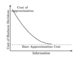
The cost of extracting information directly increases with the DataFrame’s size and complexity of the data. If I have 10 sales values, then my data set is small and simple. Minimal information, such as the mean, standard deviation, and range, can be extracted. The cost of extraction is low; just a hand-held calculator is needed. If I have $10 \mathrm{~GB}$ of data, then more can be done but at a greater cost. For data sizes approaching exabytes, the costs are monumental.

There could be an infinite amount of information, even contradictory information, in a large and complex DataFrame. So, when something is extracted, you have to check for its accuracy. For example, suppose you extract information that classifies customers by risk of default on extended credit. This particular classification may not be a good or correct one; that is, the predictive classifier $(P C)$ may not be the best one for determining whether someone is a credit risk or not. Predictive Error Analysis $(P E A)$ is needed to determine how well the $P C$ worked. I discuss this in Chap. 11. In that discussion, I will use a distinction between a training data set and a testing data set for building the classifier and testing it. This means the entire DataFrame will not, and should not, be used for a particular problem. It should be divided into the two parts although that division is not always clear, or even feasible. I will discuss the split into training and testing data sets in Chap.9.
The complexity of the DataFrame is, as I mentioned above, dependent on the types of data. Generally speaking, there are two forms: text and numeric. Other forms such as images and audio are possible but I will restrict myself to these two forms. I have to discuss these data types so that you know the possibilities and their importance and implications. How the two are handled within a DataFrame and with what statistical, econometric, and machine learning tools for the extraction of information is my focus in this book and so I will deal with them in depth in succeeding chapters. I will first discuss text data and then numeric data in the next two subsections.

商业分析代写

商科代写|商业分析作业代写Statistical Modelling for Business代考|The Data Component

讨论数据的一个共同出发点是它们是事实。关于什么是事实，有大量的哲学文献。正如 Mulligan 和 Correia（2020 年）所指出的，事实是理论和价值的对立面，并且“要与事物区分开来，特别是与复杂的对象、复合物和整体以及关系区分开来。” 在不进入这种事实哲学的情况下，我会认为事实是可检查或可证明的实体，因此是真实的。例如，华盛顿特区是美国的首都是真实的：它很容易验证并且可以被证明是真实的。这也是事实1+1=2. 这可以通过简单地计算左手的一根手指和右手的一根手指来检查。3

你可能有很多关于某个主题的事实，但如果不是，它们就没有什么价值

有组织的，
子集，
操纵，和
以有意义的方式进行解释
，以提供对行动建议的洞察力，行动就是问题的解决方案。否则，事实只是一堆毫无价值的东西。它们的价值源于您可以用它们做什么。

组织数据或事实是任何分析过程和信息驱动的第一步。这可能涉及按时间顺序（例如，按交易的日期和时间）、空间顺序（例如，北半球和南半球的国家/地区）、字母数字顺序、大小顺序等以无数种方式排列它们。例如，交易数据是关于一系列产品的销售单位的事实，包括产品种类、购买者、销售时间、销售量和价格。它们通常保存在一个没有明显顺序的文件中：只有产品、日期和单位。这些数据没有任何洞察力或情报。事实上，它是根据下订单的时间随机组织的。4然而，如果按产品和日期排序，那么它们是有条理和有用的，但并不多。最好的组织是最适用于实际问题的组织。
在数据科学、统计学、计量经济学、机器学习和其他定量领域，一种常见的组织形式是由行和列组成的矩形数组：行通常是对象，列通常是变量或特征。对象可以是人（例如，客户）或事件（例如，交易）。对象、案例、个体、事件、观察和实例这些词经常互换使用，我当然会这样做。对于本书中考虑的方法，每一行都是一个个案，每行一个案例，每个案例都在它自己的行中。

商科代写|商业分析作业代写Statistical Modelling for Business代考|The Extractor Component

最后，您必须对 DataFrame 应用一些方法或过程来提取信息。回头再看图1.2Extractor函数在信息链中的作用和位置。整本书都与这些方法有关。在我开发和讨论这些方法时，将说明对结果赋予信息意义的解释，但最终解释取决于你根据你的问题、你的领域知识和你的专业知识。

由于现代商业数据集的规模和复杂性，至少可以说，隐藏在其中的信息量和类型都很大。没有一种信息可以解决所有业务问题，没有一种方法可以解决所有问题。同一数据集可用于多个问题，并可产生多种类型的信息。可能性是无止境。然而，信息内容是您最终使用的 DataFrame 的大小和复杂性的函数。大小是数据元素的数量。由于 DataFrame 是一个矩形数组，因此大小为 #rows×#columns 元素并由其 shape 属性给出。形状表示为一个元组，写为（行，列）。例如，它可能是(5,2)对于具有 5 行和 2 列以及 10 个元素的 DataFrame。复杂性在于 DataFrame 中的数据类型，除了统计类型外很难量化。它们可以是浮点数（或简称为浮点数）、整数（或整数）、布尔值、文本字符串（称为对象）、日期时间值等。DataFrame 越大越复杂，您可以提取的信息就越多。让我=我形成，小号=大小和C=复杂。然后信息=F(小号,C)和∂我/∂小号>0和∂我/∂C>0. 对于一个非常庞大、复杂的DataFrame，信息量非常大。

提取信息的成本直接随着 DataFrame 的大小和数据的复杂性而增加。如果我有 10 个销售值，那么我的数据集很小而且很简单。可以提取最少的信息，例如均值、标准差和范围。开采成本低；只需要一个手持式计算器。如果我有10 G乙的数据，那么可以做更多的事情，但成本更高。对于接近 EB 的数据大小，成本是巨大的。

在一个庞大而复杂的 DataFrame 中，可能存在无限量的信息，甚至是相互矛盾的信息。因此，当提取某些内容时，您必须检查其准确性。例如，假设您提取按延期信贷违约风险对客户进行分类的信息。这个特定的分类可能不是一个好的或正确的分类；也就是说，预测分类器(PC)可能不是确定某人是否存在信用风险的最佳方法。预测误差分析(P和一个)需要确定如何以及PC工作了。我在第 1 章讨论这个问题。11. 在那次讨论中，我将使用训练数据集和测试数据集之间的区别来构建分类器和测试它。这意味着整个 DataFrame 不会也不应该用于解决特定问题。它应该分为两部分，尽管这种划分并不总是很清楚，甚至不可行。我将在第 9 章讨论训练和测试数据集的拆分。
正如我上面提到的，DataFrame 的复杂性取决于数据的类型。一般来说，有两种形式：文本和数字。图像和音频等其他形式也是可能的，但我将限制自己使用这两种形式。我必须讨论这些数据类型，以便您了解可能性及其重要性和含义。如何在 DataFrame 中处理这两者以及使用哪些统计、计量经济学和机器学习工具来提取信息是本书的重点，因此我将在后续章节中深入讨论它们。在接下来的两小节中，我将首先讨论文本数据，然后再讨论数字数据。

商科代写|商业分析作业代写Statistical Modelling for Business代考请认准statistics-lab™

统计代写请认准statistics-lab™. statistics-lab™为您的留学生涯保驾护航。统计代写|python代写代考

随机过程代考

在概率论概念中，随机过程是随机变量的集合。若一随机系统的样本点是随机函数，则称此函数为样本函数，这一随机系统全部样本函数的集合是一个随机过程。实际应用中，样本函数的一般定义在时间域或者空间域。 随机过程的实例如股票和汇率的波动、语音信号、视频信号、体温的变化，随机运动如布朗运动、随机徘徊等等。

贝叶斯方法代考

贝叶斯统计概念及数据分析表示使用概率陈述回答有关未知参数的研究问题以及统计范式。后验分布包括关于参数的先验分布，和基于观测数据提供关于参数的信息似然模型。根据选择的先验分布和似然模型，后验分布可以解析或近似，例如，马尔科夫链蒙特卡罗 (MCMC) 方法之一。贝叶斯统计概念及数据分析使用后验分布来形成模型参数的各种摘要，包括点估计，如后验平均值、中位数、百分位数和称为可信区间的区间估计。此外，所有关于模型参数的统计检验都可以表示为基于估计后验分布的概率报表。

广义线性模型代考

广义线性模型（GLM）归属统计学领域，是一种应用灵活的线性回归模型。该模型允许因变量的偏差分布有除了正态分布之外的其它分布。

statistics-lab作为专业的留学生服务机构，多年来已为美国、英国、加拿大、澳洲等留学热门地的学生提供专业的学术服务，包括但不限于Essay代写，Assignment代写，Dissertation代写，Report代写，小组作业代写，Proposal代写，Paper代写，Presentation代写，计算机作业代写，论文修改和润色，网课代做，exam代考等等。写作范围涵盖高中，本科，研究生等海外留学全阶段，辐射金融，经济学，会计学，审计学，管理学等全球99%专业科目。写作团队既有专业英语母语作者，也有海外名校硕博留学生，每位写作老师都拥有过硬的语言能力，专业的学科背景和学术写作经验。我们承诺100%原创，100%专业，100%准时，100%满意。

机器学习代写

随着AI的大潮到来，Machine Learning逐渐成为一个新的学习热点。同时与传统CS相比，Machine Learning在其他领域也有着广泛的应用，因此这门学科成为不仅折磨CS专业同学的“小恶魔”，也是折磨生物、化学、统计等其他学科留学生的“大魔王”。学习Machine learning的一大绊脚石在于使用语言众多，跨学科范围广，所以学习起来尤其困难。但是不管你在学习Machine Learning时遇到任何难题，StudyGate专业导师团队都能为你轻松解决。

多元统计分析代考

基础数据: $N$ 个样本， $P$ 个变量数的单样本，组成的横列的数据表
变量定性: 分类和顺序；变量定量：数值
数学公式的角度分为: 因变量与自变量

时间序列分析代写

随机过程，是依赖于参数的一组随机变量的全体，参数通常是时间。随机变量是随机现象的数量表现，其时间序列是一组按照时间发生先后顺序进行排列的数据点序列。通常一组时间序列的时间间隔为一恒定值（如1秒，5分钟，12小时，7天，1年），因此时间序列可以作为离散时间数据进行分析处理。研究时间序列数据的意义在于现实中，往往需要研究某个事物其随时间发展变化的规律。这就需要通过研究该事物过去发展的历史记录，以得到其自身发展的规律。

回归分析代写

多元回归分析渐进（Multiple Regression Analysis Asymptotics）属于计量经济学领域，主要是一种数学上的统计分析方法，可以分析复杂情况下各影响因素的数学关系，在自然科学、社会和经济学等多个领域内应用广泛。

MATLAB代写

MATLAB 是一种用于技术计算的高性能语言。它将计算、可视化和编程集成在一个易于使用的环境中，其中问题和解决方案以熟悉的数学符号表示。典型用途包括：数学和计算算法开发建模、仿真和原型制作数据分析、探索和可视化科学和工程图形应用程序开发，包括图形用户界面构建MATLAB 是一个交互式系统，其基本数据元素是一个不需要维度的数组。这使您可以解决许多技术计算问题，尤其是那些具有矩阵和向量公式的问题，而只需用 C 或 Fortran 等标量非交互式语言编写程序所需的时间的一小部分。MATLAB 名称代表矩阵实验室。MATLAB 最初的编写目的是提供对由 LINPACK 和 EISPACK 项目开发的矩阵软件的轻松访问，这两个项目共同代表了矩阵计算软件的最新技术。MATLAB 经过多年的发展，得到了许多用户的投入。在大学环境中，它是数学、工程和科学入门和高级课程的标准教学工具。在工业领域，MATLAB 是高效研究、开发和分析的首选工具。MATLAB 具有一系列称为工具箱的特定于应用程序的解决方案。对于大多数 MATLAB 用户来说非常重要，工具箱允许您学习和应用专业技术。工具箱是 MATLAB 函数（M 文件）的综合集合，可扩展 MATLAB 环境以解决特定类别的问题。可用工具箱的领域包括信号处理、控制系统、神经网络、模糊逻辑、小波、仿真等。

R语言代写	问卷设计与分析代写
PYTHON代写	回归分析与线性模型代写
MATLAB代写	方差分析与试验设计代写
STATA代写	机器学习/统计学习代写
SPSS代写	计量经济学代写
EVIEWS代写	时间序列分析代写
EXCEL代写	深度学习代写
SQL代写	各种数据建模与可视化代写

商科代写|商业分析作业代写Statistical Modelling for Business代考|STAT4600

Posted on 2022年12月14日2022年12月14日 by statistics-lab

如果你也在怎样代写商业分析Statistical Modelling for Business这个学科遇到相关的难题，请随时右上角联系我们的24/7代写客服。

商业分析就是利用数据分析和统计的方法，来分析企业之前的商业表现，从而通过分析结果来对未来的商业战略进行预测和指导。

我们提供的商业分析Statistical Modelling for Business及其相关学科的代写，服务范围广, 其中包括但不限于:

Statistical Inference 统计推断
Statistical Computing 统计计算
Advanced Probability Theory 高等楖率论
Advanced Mathematical Statistics 高等数理统计学
(Generalized) Linear Models 广义线性模型
Statistical Machine Learning 统计机器学习
Longitudinal Data Analysis 纵向数据分析
Foundations of Data Science 数据科学基础

商科代写|商业分析作业代写Statistical Modelling for Business代考|STAT4600

商科代写|商业分析作业代写Statistical Modelling for Business代考|Uncertainty vs. Risk

Uncertainty is a fact of life reflecting our lack of knowledge. It is either spatial (“I don’t know what is happening in Congress today.”) or temporal (“I don’t know what will happen to sales next year.”). In either case, the lack of knowledge is about the state of the world (SOW): what is happening in Congress and what will happen next year. Business textbooks such as Freund and Williams (1969), Spurr and Bonini (1968), and Hildebrand et al. (2005) typically discuss assigning a probability to different $S O W$ s that you could list. The purpose of these probabilities is to enable you to say something about the world before that something materializes. Somehow, and it is never explained how, you assign numeric values representing outcomes, or payoffs, to the $S O W \mathrm{~s}$. The probabilities and associated payoffs are used to calculate an expected or average payoff over all the possible $S O W$ s. Consider, for example, the rate of return on an investment (ROI) in a capital expansion project. The ROI might depend on the average annual growth of real GDP for the next 5 years. Suppose the real GDP growth is simply expressed as declining (i.e., a recession), flat ( $0 \%$ ), slow $(1 \%-2 \%)$, and robust $(>2 \%)$ with assigned probabilities of $0.05,0.20,0.50$, and $0.25$, respectively. These form a probability distribution. Let $p_i$ be the probability state $i$ is realized. Then, $\sum_{i=1}^n p_i=1.0$ for these $n=4$ possible states. I show the $S O W \mathrm{~s}$, probabilities, and $R O I$ values in Table 1.1. The expected $R O I$ is $\sum_{i=1}^4 p_i \times$ $R O I_i=2.15 \%$. This is the amount expected to be earned on average over the next 5 years.

Savage (1972, p. 9) notes that the “world” in the statement “state of the world” is defined for the problem at hand and that you should not take it literally. It is a fluid concept. He states that it is “the object about which the person is concerned.” At the same time, the “state” of the world is a full description of its conditions. Savage (1972) notes that it is “a description of the world, leaving no relevant aspects undescribed.” But he also notes that there is a true state, a “state that does in fact obtain, i.e., the true description of the world.” Unfortunately, it is unknown, and so the best we can do until it is realized or revealed to us is assign probabilities to the occurrence of each state for decision making. These are the probabilities in Table 1.1. More importantly, it is the fact that the true state is unknown, and never will be known until revealed that is the problem. No amount of information will ever completely and perfectly reveal this true state before it occurs.

商科代写|商业分析作业代写Statistical Modelling for Business代考|The Data-Information Nexus

To an extent, discussing definitions and terminology is useful for the advancement of scientific and practical solutions for any problem. If you cannot agree on basic terms, then you are doomed at worst and hindered at best from making any progress toward a solution, a decision. You can, however, become so involved in defining terms and so overly concerned about terminology that nothing else maters. Popper too strongly, that
One should never quarrel about words, and never get involved in questions of terminology … What we are really interested in, our real problem,… are problems of theories and their truth.
Popper, a philosopher of science, was concerned about scientific problems. The same sentiment, however, holds for practical problems like the ones you face daily in your business. Despite Popper’s preeminence, you still need some perspective on the foundational units that drive the raison d’etre of BDA: data and information. ${ }^1$ If information is so important for reducing uncertainty, then a logical question to ask is: “What is information?” A subordinate, but equally important, question is:

The words information and data are used as synonyms in everyday conversations. It is not uncommon, for example, to hear a business manager claim in one instance that she has a lot of data and then say in the next instance that she has a lot of information, thus linking the two words to have the same meaning. In fact, the computer systems that manage data are referred to as Information Systems (IS) and the associated technology used in those systems is referred to as Information Technology (IT). ${ }^2$ The C-Level executive in charge of this data and $I T$ infrastructure is the Chief Information Officer $(\mathrm{CIO})$. Notice the repeated use of the word “information.”
Even though people use these two words interchangeably it does not mean they have the same meaning. It is my contention, along with others, that data and information are distinct terms that, yet, have a connection. I will simply state that data are facts, objects that are true on their face, that have to be organized and manipulated to yield insight into something previously unknown. When managed and manipulated, they become information. The organization cannot be without the manipulation and the manipulation cannot be without the organization. The IT group of your business organizes your company’s data but it does not manipulate it to be information. The information is latent, hidden inside the data and must be extracted so it can be used in a decision. I illustrate this connection Fig. 1.2. I will comment on each component in the next few sections.

商业分析代写

商科代写|商业分析作业代写Statistical Modelling for Business代考|Uncertainty vs. Risk

不确定性是反映我们缺乏知识的生活事实。它要么是空间的（“我不知道今天国会发生了什么。”），要么是时间的（“我不知道明年的销售会发生什么。”）。无论哪种情况，知识的缺乏都与世界状况 (SOW) 有关：国会正在发生的事情以及明年将发生的事情。Freund 和 Williams (1969)、Spurr 和 Bonini (1968) 以及 Hildebrand 等人的商业教科书。(2005) 通常讨论将概率分配给不同的小号欧在这就是你可以列出的。这些概率的目的是使您能够在某事具体化之前对世界说些什么。不知何故，从未解释过如何将代表结果或收益的数值分配给小号欧在秒. 概率和相关的收益用于计算所有可能的预期收益或平均收益小号欧在秒。例如，考虑资本扩张项目的投资回报率 (ROI)。投资回报率可能取决于未来 5 年实际 GDP 的年均增长率。假设实际 GDP 增长简单地表示为下降（即衰退）、持平（0%），减缓(1%−2%), 并且健壮(>2%)具有指定的概率0.05,0.20,0.50，和0.25，分别。这些形成了概率分布。让p一世是概率状态一世实现了。然后，∑一世=1np一世=1.0对于这些n=4可能的状态。我展示了小号欧在秒、概率和R欧我表 1.1 中的值。预期的R欧我是∑一世=14p一世× R欧我一世=2.15%. 这是未来 5 年平均预期赚取的金额。

Savage (1972, p. 9) 指出，“世界状况”陈述中的“世界”是为手头的问题定义的，你不应该从字面上理解它。这是一个流动的概念。他说这是“这个人所关心的对象”。同时，世界的“状态”是对其状况的完整描述。Savage (1972) 指出它是“对世界的描述，没有留下任何未描述的相关方面”。但他也指出存在一种真实的状态，一种“确实获得的状态，即对世界的真实描述”。不幸的是，它是未知的，因此在它被实现或揭示给我们之前我们能做的最好的事情就是为每个状态的发生分配概率以进行决策。这些是表 1.1 中的概率。更重要的是，真实状态不明，在发现问题所在之前永远不会为人所知。在这种真实状态发生之前，再多的信息也无法完全、完美地揭示它。

商科代写|商业分析作业代写Statistical Modelling for Business代考|The Data-Information Nexus

在某种程度上，讨论定义和术语有助于为任何问题提出科学和实用的解决方案。如果你们不能就基本条款达成一致，那么最坏的情况下你注定失败，最好的情况下你也无法在解决方案和决策方面取得任何进展。但是，您可能会过多地参与定义术语并过分关注术语，而忽略了其他任何事情。波普尔太强烈了，
一个人永远不应该为词语争吵，永远不要卷入术语问题……我们真正感兴趣的，我们真正的问题，……是理论及其真理的问题。
科学哲学家波普尔关注科学问题。然而，同样的观点也适用于实际问题，例如您在业务中每天面临的问题。尽管 Popper 非常出色，但您仍然需要对驱动 BDA 存在理由的基本单元有一些看法：数据和信息。1如果信息对于减少不确定性如此重要，那么一个合乎逻辑的问题是：“什么是信息？” 一个从属但同样重要的问题是：

信息和数据这两个词在日常对话中用作同义词。例如，经常听到一位业务经理在一个实例中声称她有很多数据，然后在下一个实例中又说她有很多信息，从而将两个词联系起来具有相同的含义。事实上，管理数据的计算机系统被称为信息系统 (IS)，这些系统中使用的相关技术被称为信息技术 (IT)。2负责此数据的 C 级主管和我吨基础设施是首席信息官(C我欧). 请注意“信息”一词的重复使用。
尽管人们可以互换使用这两个词，但这并不意味着它们具有相同的含义。我和其他人的观点是，数据和信息是不同的术语，但它们之间存在联系。我将简单地说明数据是事实，是表面上真实的对象，必须对其进行组织和操作以深入了解以前未知的事物。当被管理和操纵时，它们就变成了信息。组织不能没有操纵，操纵也不能没有组织。您企业的 IT 团队组织您公司的数据，但不会将其处理为信息。信息是潜在的，隐藏在数据中，必须提取出来才能用于决策。我在图 1.2 中说明了这种连接。

统计代写请认准statistics-lab™. statistics-lab™为您的留学生涯保驾护航。统计代写|python代写代考

随机过程代考

贝叶斯方法代考

广义线性模型代考

广义线性模型（GLM）归属统计学领域，是一种应用灵活的线性回归模型。该模型允许因变量的偏差分布有除了正态分布之外的其它分布。

机器学习代写

多元统计分析代考

基础数据: $N$ 个样本， $P$ 个变量数的单样本，组成的横列的数据表
变量定性: 分类和顺序；变量定量：数值
数学公式的角度分为: 因变量与自变量

时间序列分析代写

回归分析代写

MATLAB代写

R语言代写	问卷设计与分析代写
PYTHON代写	回归分析与线性模型代写
MATLAB代写	方差分析与试验设计代写
STATA代写	机器学习/统计学习代写
SPSS代写	计量经济学代写
EVIEWS代写	时间序列分析代写
EXCEL代写	深度学习代写
SQL代写	各种数据建模与可视化代写

商科代写|商业分析作业代写Statistical Modelling for Business代考|DATA603

Posted on 2022年12月14日2022年12月14日 by statistics-lab

如果你也在怎样代写商业分析Statistical Modelling for Business这个学科遇到相关的难题，请随时右上角联系我们的24/7代写客服。

商业分析就是利用数据分析和统计的方法，来分析企业之前的商业表现，从而通过分析结果来对未来的商业战略进行预测和指导。

我们提供的商业分析Statistical Modelling for Business及其相关学科的代写，服务范围广, 其中包括但不限于:

Statistical Inference 统计推断
Statistical Computing 统计计算
Advanced Probability Theory 高等楖率论
Advanced Mathematical Statistics 高等数理统计学
(Generalized) Linear Models 广义线性模型
Statistical Machine Learning 统计机器学习
Longitudinal Data Analysis 纵向数据分析
Foundations of Data Science 数据科学基础

商科代写|商业分析作业代写Statistical Modelling for Business代考|DATA603

商科代写|商业分析作业代写Statistical Modelling for Business代考|Types of Business Problems

What types of business problems warrant $B D A$ ? The types are too numerous to mention, but to give a sense of them consider a few examples:

Anomaly Detection: production surveillance, predictive maintenance, manufacturing yield optimization;
Fraud detection;
Identity theft;
Account and transaction anomalies;
Customer analytics:
Customer Relationship Management (CRM);
Churn analysis and prevention;
Customer Satisfaction;
Marketing cross-sell and up-sell;
Pricing: leakage monitoring, promotional effects tracking, competitive price responses;
Fulfillment: management and pipeline tracking;
Competitive monitoring;
Competitive Environment Analysis (CEA); and
New Product Development.
And the list goes on, and on.
A decision of some type is required for all these problems. New product development best exemplifies a complex decision process. Decisions are made throughout a product development pipeline. This is a series of stages from ideation or conceptualization to product launch and post-launch tracking. Paczkowski (2020) identifies five stages for a pipeline: ideation, design, testing, launch, and post-launch tracking. Decisions are made between each stage whether to proceed to the next one or abort development or even production. Each decision point is marked by a business case analysis that examines the expected revenue and market share for the product. Expected sales, anticipated price points (which are refined as the product moves through the pipeline), production and marketing cost estimates, and competitive analyses that include current products, sales, pricing, and promotions plus competitive responses to the proposed new product, are all needed for each business case assessment. If any of these has a negative implication for the concept, then it will be canceled and removed from the pipeline. Information is needed for each business case check point.

The expected revenue and market share are refined for each business case analysis as new and better information -not data-become available for the items I listed above. More data do become available, of course, as the product is developed, but it is the analysis of that data based on methods described in this book, that provide the information needed to approve or not approve the advancement of the concept to the next stage in the pipeline. The first decision, for example, is simply to begin developing a new product. Someone has to say “Yes” to the question “Should we develop a new product?” The business case analysis provides that decision maker with the information for this initial “Go/No Go” decision. Similar decisions are made at other stages.

Another example is product pricing. This is actually a two-fold decision involving a structure (e.g., uniform pricing or price discrimination to mention two possibilities) and a level within the structure. These decisions are made throughout the product life cycle beginning at the development stage (the launch stage of the pipeline I discussed above) and then throughout the post-launch period until the product is ultimately removed from the market. The wrong price structure and/or level could cost your business lost profit, lost market share, or a lost business. See Paczkowski (2018) for a discussion of the role of pricing and the types of analysis for identifying the best price structure and level. Also see Paczkowski (2020) for new product development pricing at each stage of the pipeline.

商科代写|商业分析作业代写Statistical Modelling for Business代考|The Role of Information in Business Decision Making

Decisions are effective if they solve a problem, such as those I discussed above, and aid rather than hinder your business in succeeding in the market. I will assume your business succeeds if it earns a profit and has a positive return for its owners (shareholders, partners, employees in an employee-owned company) or a sole owner. Information could be about

current sales;
future sales;
the state of the market;
consumer, social, and technology trends and developments;
customer needs and wants;
customer willingness-to-pay;
key customer segments;
financial developments;
supply chain developments; and
the size of customer churn.
This information is input into decisions and like any input, if it is bad, then the decisions will be bad. Basically, the GIGO Principle (Garbage In-Garbage Out) holds. This should be obvious and almost trite. Unfortunately, you do not know when you make your decision if your information is good or bad, or even sufficient. You face uncertainty due to the amount and quality of the information you have available.

Without any information you would just be guessing, and guessing is costly. In Fig. 1.1, I illustrate what happens to the cost of decisions based on the amount of information you have. Without any information, all your decisions are based on pure guesses, hunches, so you are forced to approximate their effect. The approximation could be very naive, based on gut instinct (i.e., an unfounded belief that you know everything) or what happened yesterday or in another business similar to yours (i.e., an analog business).

The cost of these approximations in terms of financial losses, lost market share, or outright bankruptcy can be very high. As the amount of information increases, however, you will have more insight so your approximations (i.e., guesses) improve and the cost of approximations declines. This is exactly what happens during the business case process I described above. More and better information helps the decision makers at each business case stage. The approximations could now be based on trends, statistically significant estimates of impact, or model-based what-if analyses. These are not “data”; they are information.

商业分析代写

商科代写|商业分析作业代写Statistical Modelling for Business代考|Types of Business Problems

什么类型的业务问题保证乙丁一个？类型太多无法一一列举，但为了让您了解它们，请考虑几个示例：

异常检测：生产监控、预测性维护、制造良率优化；
欺诈识别;
身份盗用；
账户及交易异常；
客户分析：
客户关系管理（CRM）；
客户流失分析与预防；
顾客满意度;
营销交叉销售和追加销售；
定价：泄漏监控、促销效果跟踪、有竞争力的价格响应；
履行：管理和管道跟踪；
竞争监控；
竞争环境分析（CEA）；和
新产品开发。
这样的例子不胜枚举。
所有这些问题都需要某种类型的决定。新产品开发最能说明复杂的决策过程。决策是在整个产品开发流程中做出的。这是从构思或概念化到产品发布和发布后跟踪的一系列阶段。Paczkowski (2020) 确定了管道的五个阶段：构思、设计、测试、发布和发布后跟踪。在每个阶段之间做出决定是继续下一阶段还是中止开发甚至生产。每个决策点都由业务案例分析标记，该分析检查产品的预期收入和市场份额。预期销售额、预期价格点（随着产品在管道中移动而细化）、生产和营销成本估算以及包括当前产品的竞争分析，每个业务案例评估都需要销售、定价和促销以及对拟议新产品的竞争性反应。如果其中任何一个对该概念有负面影响，那么它将被取消并从管道中删除。每个业务案例检查点都需要信息。

随着新的和更好的信息（不是数据）可用于我上面列出的项目，每个业务案例分析的预期收入和市场份额都得到了改进。当然，随着产品的开发，确实会有更多数据可用，但正是基于本书描述的方法对这些数据进行的分析，提供了批准或不批准将概念推进到下一阶段所需的信息在管线中。例如，第一个决定就是开始开发新产品。有人必须对“我们应该开发新产品吗？”这个问题说“是”。商业案例分析为决策者提供了这个最初的“通过/不通过”决策的信息。在其他阶段也会做出类似的决定。

另一个例子是产品定价。这实际上是一个双重决策，涉及结构（例如，统一定价或价格歧视两种可能性）和结构内的级别。这些决策是在整个产品生命周期中做出的，从开发阶段（我上面讨论的管道的启动阶段）开始，然后在整个启动后阶段，直到产品最终退出市场。错误的价格结构和/或水平可能会使您的企业损失利润、失去市场份额或失去业务。请参阅 Paczkowski (2018) 讨论定价的作用以及用于确定最佳价格结构和水平的分析类型。另请参阅 Paczkowski (2020) 了解管道每个阶段的新产品开发定价。

商科代写|商业分析作业代写Statistical Modelling for Business代考|The Role of Information in Business Decision Making

如果决策能够解决问题（例如我上面讨论的问题）并且有助于而不是阻碍您的企业在市场上取得成功，那么决策就是有效的。如果您的企业盈利并为其所有者（股东、合伙人、员工持股公司的员工）或唯一所有者带来正回报，我会假设您的企业成功。信息可能是关于

当前销售额；
未来的销售；
市场状况；
消费者、社会和技术趋势和发展；
客户的需求和愿望；
客户支付意愿；
关键客户群；
金融发展；
供应链发展；和
客户流失的规模。
这些信息被输入到决策中，就像任何输入一样，如果它是错误的，那么决策就会是错误的。基本上，GIGO 原则（垃圾进垃圾出）成立。这应该是显而易见的，几乎是陈腐的。不幸的是，您不知道您何时做出决定，您的信息是好是坏，甚至是充分的。由于可用信息的数量和质量，您面临着不确定性。

如果没有任何信息，您将只能猜测，而猜测的代价是昂贵的。在图 1.1 中，我说明了基于您拥有的信息量的决策成本会发生什么变化。在没有任何信息的情况下，你所有的决定都是基于纯粹的猜测和直觉，所以你不得不估计它们的效果。近似值可能非常天真，基于直觉（即毫无根据地相信你知道一切）或昨天发生的事情或在与你的业务类似的另一家公司（即模拟公司）中发生的事情。

这些近似值在财务损失、市场份额损失或彻底破产方面的成本可能非常高。但是，随着信息量的增加，您将获得更多洞察力，因此您的近似值（即猜测）会得到改善，而近似值的成本会下降。这正是我在上面描述的业务案例过程中发生的事情。更多更好的信息有助于每个业务案例阶段的决策者。这些近似值现在可以基于趋势、具有统计意义的影响估计或基于模型的假设分析。这些不是“数据”；他们是信息。

统计代写|商业分析作业代写Statistical Modelling for Business代考请认准statistics-lab™

统计代写请认准statistics-lab™. statistics-lab™为您的留学生涯保驾护航。统计代写|python代写代考

随机过程代考

贝叶斯方法代考

广义线性模型代考

广义线性模型（GLM）归属统计学领域，是一种应用灵活的线性回归模型。该模型允许因变量的偏差分布有除了正态分布之外的其它分布。

机器学习代写

多元统计分析代考

基础数据: $N$ 个样本， $P$ 个变量数的单样本，组成的横列的数据表
变量定性: 分类和顺序；变量定量：数值
数学公式的角度分为: 因变量与自变量

时间序列分析代写

回归分析代写

MATLAB代写

R语言代写	问卷设计与分析代写
PYTHON代写	回归分析与线性模型代写
MATLAB代写	方差分析与试验设计代写
STATA代写	机器学习/统计学习代写
SPSS代写	计量经济学代写
EVIEWS代写	时间序列分析代写
EXCEL代写	深度学习代写
SQL代写	各种数据建模与可视化代写

商科代写|计量经济学代写Econometrics代考|Best 27

Posted on 2022年7月22日2022年7月22日 by statistics-lab

如果你也在怎样代写计量经济学Econometrics这个学科遇到相关的难题，请随时右上角联系我们的24/7代写客服。

计量经济学，对经济关系的统计和数学分析，通常作为经济预测的基础。这种信息有时被政府用来制定经济政策，也被私人企业用来帮助价格、库存和生产方面的决策。

statistics-lab™ 为您的留学生涯保驾护航在代写计量经济学Econometrics方面已经树立了自己的口碑, 保证靠谱, 高质且原创的统计Statistics代写服务。我们的专家在代写计量经济学Econometrics代写方面经验极为丰富，各种代写计量经济学Econometrics相关的作业也就用不着说。

我们提供的计量经济学Econometrics及其相关学科的代写，服务范围广, 其中包括但不限于:

Statistical Inference 统计推断
Statistical Computing 统计计算
Advanced Probability Theory 高等概率论
Advanced Mathematical Statistics 高等数理统计学
(Generalized) Linear Models 广义线性模型
Statistical Machine Learning 统计机器学习
Longitudinal Data Analysis 纵向数据分析
Foundations of Data Science 数据科学基础

商科代写|计量经济学代写Econometrics代考|Formal Tests for Serial Correlation

The Durbin-Watson (DW) test provides a formal test in which the null hypothesis is that the equation errors are serially uncorrelated and the alternative is that they follow a first-order autocorrelation process. This test was first introduced by Durbin and Watson in two papers published in Biometrika in 1950 and 1951 [Durbin1950] and [Durbin1951]. It is a standard part of the regression output for most econometrics packages. The DW test builds on a previous test developed by Von Neumann [VonNeumann1941] who developed a test for autocorrelation in a series of random variables with the null that the variables are independent random numbers. Unfortunately, this is not suitable when the series under examination comprises regression residuals, which are not independent by construction. Although Von Neumann’s statistic has a relatively simple distribution, that is, the standard normal distribution, Durbin and Watson showed that the distribution of their test statistic was necessarily more complex. The nature of the test statistic means that it is not possible to derive unique critical values for a test of the null of no autocorrelation against the alternative of first-order autocorrelation. However, they did demonstrate that the critical values for their test were bounded and were able to tabulate the bounds for small sample sizes.
The DW test is concerned with a specific form of serial correlation, that is, first-order autocorrelation but is arguably sensitive to other forms. Consider the following regression model with an error that follows an AR process of order one:
$$
\begin{aligned}
&Y_{t}=\beta X_{t}+u_{t} \
&u_{t}=\rho u_{t-1}+\varepsilon_{t} .
\end{aligned}
$$
Taking the residuals from an OLS regression of $Y$ on $X$, we can construct the test statistic
$$
D W=\sum_{t=2}^{T}\left(\hat{u}{t}-\hat{u}{t-1}\right)^{2} / \sum_{t=1}^{T} \hat{u}_{t}^{2} .
$$

商科代写|计量经济学代写Econometrics代考|DEALING WITH SERIAL CORRELATION

If serial correlation is present, then there are several ways to deal with the issue. Of course, the priority is to identify the nature, and hopefully the cause, of the serial correlation. If the root cause of the problem is the omission of a relevant variable from the model, then the natural solution is to include that variable. If it is determined that modeling of the serial correlation process is appropriate, then we have several different methods available for the estimation of such models by adjusting for the presence of serially correlation errors. It should be noted that mechanical adjustments, of the type we will describe in this section, are potentially dangerous. This process has been much criticized on the grounds that there is a risk that these methods disguise an underlying problem rather than dealing with it. McGuirk and Spanos [McGuirk2009] are particularly critical of mechanical adjustments to deal with autocorrelated arguments. In this paper, they show that unless we can assume that the regress and does not Granger-cause the regressors, adjusting for autocorrelation means that least squares yield biased and inconsistent estimates. However, these methods are still used and reported in applied work and it is therefore important that we consider how they work.

The first method we will consider is that of Cochrane-Orcutt estimation. This uses an iterative algorithm proposed by Cochrane and Orcutt [Cochrane1949] in which we use the structure of the problem to separate out the estimation of the behavioral parameters of the main equation from those of the AR process that describes the errors. Let us consider the case of an $\mathrm{AR}(1)$ error process as an example. Suppose we wish to estimate a model of the form (5.6). The two equations can be combined to give a single equation of the form
$$
Y_{t}-\rho Y_{t-1}=\beta\left(X_{t}-\rho X_{t-1}\right)+\varepsilon_{t},
$$
that is, an equation in “quasi-differences” of the data. If $\rho$ was known, then it would be straightforward to construct these quasi-differences and estimate the behavioral parameter $\beta$ by least squares. In the absence of such knowledge, we make a guess at $\rho$ and construct an estimate of $\beta$ on this basis. We then generate the residuals $\hat{u}{t}=Y{t}-\beta X_{t}$ on this basis and calculate an estimate of $\rho$ of the form $\hat{\rho}=\sum_{t=2}^{T} \hat{u}{t} \hat{u}{t-1} / \sum_{t=1}^{T} \hat{u}_{t}^{2}$. If, by some lucky chance, this estimate coincides with our assumption, then we stop. Otherwise, we use our estimate to recalculate the quasi-differences, reestimate $\beta$, and continue until our estimates of $\beta$ and $p$ converge. If a solution exists, then this provides a robust algorithm for estimation.

计量经济学代考

商科代写|计量经济学代写Econometrics代考|Formal Tests for Serial Correlation

Durbin-Watson (DW) 检验提供了一种形式检验，其中零假设是方程误差是序列不相关的，而另一种方法是它们遵循一阶自相关过程。该测试由 Durbin 和 Watson 在 1950 年和 1951 年在 Biometrika 发表的两篇论文 [Durbin1950] 和 [Durbin1951] 中首次引入。它是大多数计量经济学软件包回归输出的标准部分。DW 测试建立在 Von Neumann [VonNeumann1941] 开发的先前测试的基础上，该测试开发了一系列随机变量的自相关测试，其中变量为独立随机数。不幸的是，当检查的序列包含回归残差时，这不适合，这些回归残差在构造上不是独立的。尽管冯诺依曼的统计量具有相对简单的分布，即标准正态分布，但 Durbin 和 Watson 表明，他们的检验统计量的分布必然更复杂。检验统计量的性质意味着不可能为无自相关的零点与一阶自相关的备选方案的检验推导出唯一的临界值。然而，他们确实证明了他们测试的临界值是有界的，并且能够将小样本的界限制表。检验统计量的性质意味着不可能为无自相关的零点与一阶自相关的备选方案的检验推导出唯一的临界值。然而，他们确实证明了他们测试的临界值是有界的，并且能够将小样本的界限制表。检验统计量的性质意味着不可能为无自相关的零点与一阶自相关的备选方案的检验推导出唯一的临界值。然而，他们确实证明了他们测试的临界值是有界的，并且能够将小样本的界限制表。

DW 检验关注特定形式的序列相关，即一阶自相关，但可以说对其他形式敏感。考虑以下回归模型，其误差遵循一阶 AR 过程:
$$
Y_{t}=\beta X_{t}+u_{t} \quad u_{t}=\rho u_{t-1}+\varepsilon_{t} .
$$
从 OLS 回归中获取残差 $Y$ 上 $X$ ，我们可以构造检验统计量
$$
D W=\sum_{t=2}^{T}(\hat{u} t-\hat{u} t-1)^{2} / \sum_{t=1}^{T} \hat{u}_{t}^{2} .
$$

商科代写|计量经济学代写Econometrics代考|DEALING WITH SERIAL CORRELATION

如果存在序列相关性，那么有几种方法可以处理该问题。当然，当务之急是确定序列相关的性质，并希望是原因。如果问题的根本原因是模型中遗漏了相关变量，那么自然的解决方案是包含该变量。如果确定序列相关过程的建模是合适的，那么我们有几种不同的方法可用于通过调整序列相关误差的存在来估计此类模型。应该注意的是，我们将在本节中描述的那种机械调整具有潜在的危险。这个过程受到了很多批评，理由是这些方法存在掩盖潜在问题而不是处理它的风险。McGuirk 和 Spanos [McGuirk2009] 特别批评机械调整以处理自相关参数。在本文中，他们表明，除非我们可以假设回归并且不是 Granger 导致回归量，否则调整自相关意味着最小二乘法会产生有偏和不一致的估计。然而，这些方法仍在应用工作中使用和报告，因此我们考虑它们的工作原理很重要。
我们将考虑的第一种方法是 Cochrane-Orcutt 估计。这使用了 Cochrane 和 Orcutt [Cochrane1949] 提出的迭代算法，其中我们使用问题的结构将主方程的行为参数的估计与描述错误的 AR 过程的估计分开。让我们考虑一个案例 $\operatorname{AR}(1)$ 以错误过程为例。假设我们布望估计一个形式为 (5.6) 的模型。这两个方程可以组合得到一个方程，形式为
$$
Y_{t}-\rho Y_{t-1}=\beta\left(X_{t}-\rho X_{t-1}\right)+\varepsilon_{t},
$$
也就是说，数据的”准差分”方程。如果 $\rho$ 是已知的，那么构建这些准差异并估计行为参数将很简单 $\beta$ 通过最小二乘。在没有这些知识的情况下，我们猜测 $\rho$ 并构建一个估计 $\beta$ 以这个为基础。然后我们生成残差 $\hat{u} t=Y t-\beta X_{t}$ 在此基础上并计算估计 $\rho$ 形式的 $\hat{\rho}=\sum_{t=2}^{T} \hat{u} t \hat{u} t-1 / \sum_{t=1}^{T} \hat{u}_{t}^{2}$. 如果碰巧这个估计与我们的假设一致，那么我们就停下来。否则，我们使用我们的估计来重新计算准差，重新估计 $\beta$ ，并继续直到我们估计 $\beta$ 和 $p$ 收敛。如果存在解决方案，则这提供了一种稳健的估计算法。

商科代写|计量经济学代写Econometrics代考请认准statistics-lab™

统计代写请认准statistics-lab™. statistics-lab™为您的留学生涯保驾护航。

金融工程代写

金融工程是使用数学技术来解决金融问题。金融工程使用计算机科学、统计学、经济学和应用数学领域的工具和知识来解决当前的金融问题，以及设计新的和创新的金融产品。

非参数统计代写

非参数统计指的是一种统计方法，其中不假设数据来自于由少数参数决定的规定模型；这种模型的例子包括正态分布模型和线性回归模型。

广义线性模型代考

广义线性模型（GLM）归属统计学领域，是一种应用灵活的线性回归模型。该模型允许因变量的偏差分布有除了正态分布之外的其它分布。

术语广义线性模型（GLM）通常是指给定连续和/或分类预测因素的连续响应变量的常规线性回归模型。它包括多元线性回归，以及方差分析和方差分析（仅含固定效应）。

有限元方法代写

有限元方法（FEM）是一种流行的方法，用于数值解决工程和数学建模中出现的微分方程。典型的问题领域包括结构分析、传热、流体流动、质量运输和电磁势等传统领域。

有限元是一种通用的数值方法，用于解决两个或三个空间变量的偏微分方程（即一些边界值问题）。为了解决一个问题，有限元将一个大系统细分为更小、更简单的部分，称为有限元。这是通过在空间维度上的特定空间离散化来实现的，它是通过构建对象的网格来实现的：用于求解的数值域，它有有限数量的点。边界值问题的有限元方法表述最终导致一个代数方程组。该方法在域上对未知函数进行逼近。[1] 然后将模拟这些有限元的简单方程组合成一个更大的方程系统，以模拟整个问题。然后，有限元通过变化微积分使相关的误差函数最小化来逼近一个解决方案。

tatistics-lab作为专业的留学生服务机构，多年来已为美国、英国、加拿大、澳洲等留学热门地的学生提供专业的学术服务，包括但不限于Essay代写，Assignment代写，Dissertation代写，Report代写，小组作业代写，Proposal代写，Paper代写，Presentation代写，计算机作业代写，论文修改和润色，网课代做，exam代考等等。写作范围涵盖高中，本科，研究生等海外留学全阶段，辐射金融，经济学，会计学，审计学，管理学等全球99%专业科目。写作团队既有专业英语母语作者，也有海外名校硕博留学生，每位写作老师都拥有过硬的语言能力，专业的学科背景和学术写作经验。我们承诺100%原创，100%专业，100%准时，100%满意。

随机分析代写

随机微积分是数学的一个分支，对随机过程进行操作。它允许为随机过程的积分定义一个关于随机过程的一致的积分理论。这个领域是由日本数学家伊藤清在第二次世界大战期间创建并开始的。

时间序列分析代写

回归分析代写

MATLAB代写

R语言代写	问卷设计与分析代写
PYTHON代写	回归分析与线性模型代写
MATLAB代写	方差分析与试验设计代写
STATA代写	机器学习/统计学习代写
SPSS代写	计量经济学代写
EVIEWS代写	时间序列分析代写
EXCEL代写	深度学习代写
SQL代写	各种数据建模与可视化代写

商科代写|计量经济学代写Econometrics代考|Best 22

Posted on 2022年7月22日2022年7月22日 by statistics-lab

如果你也在怎样代写计量经济学Econometrics这个学科遇到相关的难题，请随时右上角联系我们的24/7代写客服。

我们提供的计量经济学Econometrics及其相关学科的代写，服务范围广, 其中包括但不限于:

Statistical Inference 统计推断
Statistical Computing 统计计算
Advanced Probability Theory 高等概率论
Advanced Mathematical Statistics 高等数理统计学
(Generalized) Linear Models 广义线性模型
Statistical Machine Learning 统计机器学习
Longitudinal Data Analysis 纵向数据分析
Foundations of Data Science 数据科学基础

商科代写|计量经济学代写Econometrics代考|DETECTION OF SERIAL CORRELATION

Since serial correlation of the errors has been shown to have important implications for our interpretation of regression results, it becomes important to develop tests for whether it is present in the models we estimate. It will be helpful to have an example in mind as we develop such tests. Consider the following estimated consumption function for the US economy based on annual data from 1970 to $2019 .$
$\ln \left(C_{t}\right)=\underset{(0.0466)}{-0.2898}+\underset{(0.0052)}{1.0174} \ln \left(Y D_{t}\right)+\hat{u}{t}$ $R^{2}=0.9987 \quad \hat{\sigma}{u}=0.0154 \quad T=50$
$D W=0.5389$,
where $C$ is total consumers’ expenditure and $Y D$ is real personal disposable income. Both variables are measured in millions of dollars at 2012 prices.
On first inspection, this equation appears to have reasonable properties. The slope coefficient is statistically significantly different from zero and the coefficient of determination indicates a good fit. In this case, however, it is more interesting to test the null hypothesis that the slope coefficient is equal to 1 . This is because the slope coefficient in this relationship measures the income elasticity of consumption expenditure. However, this null hypothesis is also rejected by our model. The $t$ statistic for this test is $(1.0174-1) / 0.0052=3.35$ which leads us to reject the null at the $5 \%$ level. This conclusion is, however, may be unreliable if the errors in this model are serially correlated. Therefore, in order to assess the robustness of our estimates of the model parameters, we need to test for the presence of serial correlation in the residuals $\hat{u}$ from equation (5.18).

商科代写|计量经济学代写Econometrics代考|Informal Tests for Serial Correlation

We can look for serial correlation informally by simply inspecting a plot of the residuals. If runs of positive or negative residuals are obvious, then this is a sign that serial correlation is present. For example, Figure $5.2$ shows the residuals for our consumption function equation and it is obvious that there are periods during which the residuals are consistently either positive or negative. This is a clear indication that the equation suffers from serial correlation. There are, however, forms of serial correlation, such as moving average errors, which are not so easily detected. Therefore, it is important to develop more formal tests as well as procedures for identifying the specific form of serial correlation that is relevant for this equation.

The correlogram 1 provides a more formal statistical method for the investigation of serial correlation. The correlogram is a table, or plot, of the sample autocorrelations of the regression residuals. The sample autocorrelations are defined in equation (5.19), and Figure $5.3$ gives both a table and a graph of the autocorrelations of the residuals from equation (5.18).
$$
\hat{\rho}{k}=\sum{t=k+1}^{T} \hat{u}{t} \hat{u}{t-k} / \sum_{t=1}^{T} \hat{u}_{t^{2}}^{2} .
$$

计量经济学代考

商科代写|计量经济学代写Econometrics代考|DETECTION OF SERIAL CORRELATION

由于误差的序列相关性已被证明对我们对回归结果的解释具有重要意义，因此开发测试它是否存在于我们估计的模型中变得很重要。在我们开发此类测试时，记住一个示例将很有帮助。根据 1970 年到 2019 . $D W=0.5389$,
其中 $C$ 是消费者总支出和 $Y D$ 是真实的个人可支配收入。这两个变量都以 2012 年的价格计算，单位为百万美元。
乍一看，这个方程似乎具有合理的性质。斜率系数在统计上显着不同于零，决定系数表明拟合良好。然而，在这种情况下，更有趣的是检验斜率系数等于 1 的原假设。这是因为该关系中的斜率系数衡量的是消费支出的收入弹性。然而，我们的模型也拒绝了这个零假设。这该测试的统计数据是 $(1.0174-1) / 0.0052=3.35$ 这导致我们在 $5 \%$ 等级。然而，如果这个模型中的误差是序列相关的，这个结论可能是不可靠的。因此，为了评估我们对模型参数估计的稳健性，我们需要测试残差中是否存在序列相关性 $u$ 从方程 (5.18)。

商科代写|计量经济学代写Econometrics代考|Informal Tests for Serial Correlation

我们可以通过简单地检查残差图来非正式地寻找序列相关性。如果正或负残差的运行很明显，那么这表明存在序列相关性。例如，图5.2显示了我们的消费函数方程的残差，很明显，在某些时期内，残差始终为正或负。这清楚地表明该方程存在序列相关性。然而，有一些序列相关的形式，例如移动平均误差，它们并不那么容易检测到。因此，重要的是开发更正式的测试以及用于识别与该方程相关的特定序列相关形式的程序。
相关图 1 为研究序列相关性提供了一种更正式的统计方法。相关图是回归残差的样本自相关的表格或图。样本自相关在方程 (5.19) 中定义，图5.3给出方程 (5.18) 中残差的自相关的表格和图表.
$$
\hat{\rho} k=\sum t=k+1^{T} \hat{u} t \hat{u} t-k / \sum_{t=1}^{T} \hat{u}_{t^{2}}^{2} .
$$

统计代写请认准statistics-lab™. statistics-lab™为您的留学生涯保驾护航。

金融工程代写

非参数统计代写

非参数统计指的是一种统计方法，其中不假设数据来自于由少数参数决定的规定模型；这种模型的例子包括正态分布模型和线性回归模型。

广义线性模型代考

广义线性模型（GLM）归属统计学领域，是一种应用灵活的线性回归模型。该模型允许因变量的偏差分布有除了正态分布之外的其它分布。

有限元方法代写

随机分析代写

时间序列分析代写

回归分析代写

MATLAB代写

R语言代写	问卷设计与分析代写
PYTHON代写	回归分析与线性模型代写
MATLAB代写	方差分析与试验设计代写
STATA代写	机器学习/统计学习代写
SPSS代写	计量经济学代写
EVIEWS代写	时间序列分析代写
EXCEL代写	深度学习代写
SQL代写	各种数据建模与可视化代写

商科代写|计量经济学代写Econometrics代考|Find 2022

Posted on 2022年7月22日2022年7月22日 by statistics-lab

如果你也在怎样代写计量经济学Econometrics这个学科遇到相关的难题，请随时右上角联系我们的24/7代写客服。

我们提供的计量经济学Econometrics及其相关学科的代写，服务范围广, 其中包括但不限于:

Statistical Inference 统计推断
Statistical Computing 统计计算
Advanced Probability Theory 高等概率论
Advanced Mathematical Statistics 高等数理统计学
(Generalized) Linear Models 广义线性模型
Statistical Machine Learning 统计机器学习
Longitudinal Data Analysis 纵向数据分析
Foundations of Data Science 数据科学基础

商科代写|计量经济学代写Econometrics代考|CAUSES OF SERIAL CORRELATION

Consider a regression equation of the standard form $Y_{t}=\beta X_{t}+u_{t}$. We assume a model in mean deviation form to simplify the notation and the discussion. The errors of this model are said to be serially correlated if $E\left(u_{t} u_{t-k}\right) \neq 0$ for some $k \neq 0$. A natural question is why the errors might be correlated in this way? For the moment, we will simply assume that this is an intrinsic property of the data. That is, we assume that shocks to the equation are not random drawings from a distribution but instead depend upon their own past values. An alternative would be to assume that correlation in the errors arises because the model is misspecified in some way. However, this would complicate much of the discussion and we will avoid this assumption for the moment, on the understanding that it will be relaxed later.

There are many different forms that serial correlation might take. For example, the errors might follow a first-order autoregressive (AR) process. This would mean that the error process could be described by an equation of the form $u_{t}=\rho u_{t-1}+\varepsilon_{t}$, where $\varepsilon_{t}$, is a truly random disturbance and $\rho \neq 0$. This is a very common and important case, but it is not the only form that serial correlation can take. An alternative is where the error term in the equation is an average over several time periods of the random disturbance $\varepsilon_{t}$. For example, we might have a first-order moving average process of the form $u_{t}=\varepsilon_{t}+\lambda \varepsilon_{t-1}$. Both error processes are said to be serially correlated but each produces different implications and problems for the modeler. However, in both cases, the problem of dealing with serial correlation is simplified because of the assumption that it is an intrinsic feature of the error themselves, that is, the problem is one of error dynamics. A more realistic conclusion might be that the errors are serially correlated because of some fundamental misspecification in the original equation.

商科代写|计量经济学代写Econometrics代考|CONSEQUENCES OF SERIAL CORRELATION

Now that we have established some of the reasons why serial correlation may arise in regression models, let us consider the implications for least squares regression analysis. Suppose we have a model in which the errors follow a first-order AR process as set out in (5.6)
$$
\begin{aligned}
&Y_{t}=\beta X_{t}+u_{t} \
&u_{t}=\rho u_{t-1}+\varepsilon_{t},
\end{aligned}
$$
where $\varepsilon_{t}, t=1, \ldots, T$ are independent, identically distributed random disturbances with mean zero and constant variance. As we have seen, this is not the only possible type of serial correlation which may arise, but the results we derive for this model apply more generally to other forms of serial correlation.

The AR process defined in (5.6) can be written in moving average form. Using the method of backward substitution, we have
$$
u_{t}=\varepsilon_{t}+\rho \varepsilon_{t-1}+\rho^{2} \varepsilon_{t-2} \ldots=\sum_{j=0}^{\infty} \rho^{j} \varepsilon_{t-j} .
$$
This is an infinite moving average process. Providing $|\rho|<1$, then the sequence defined in (5.7) will converge, in the sense that it will have a finite variance. To see this note that
$$
E\left(u_{t}^{2}\right)=\sum_{j=0}^{\infty} \rho^{2 j} E\left(\varepsilon_{t-j}^{2}\right)=\sum_{j=0}^{\mu_{j}} \rho^{2 j} \sigma_{\varepsilon}^{2}=\frac{\sigma_{\varepsilon}^{2}}{1-\rho^{2}}
$$
Therefore, for the variance of the error term to be finite and positive, we need $|\rho|<1$. If this condition holds, then the process is said to be weakly stationary and it can be shown that a general feature of stationary, finite AR processes is that they can be written as infinite moving average processes. Moreover, since $E\left(\varepsilon_{t-j}\right)=0$ for all values of $j$, it follows that $E\left(u_{t}\right)=0$. This is a useful property because we have already seen that the expected value of the OLS estimator can be written as follows: $E(\hat{\beta})=\beta+\sum_{t=1}^{T} X_{t} E\left(u_{t}\right) / \sum_{t=1}^{T} X_{t}^{2}$. It therefore follows that $E(\hat{\beta})=\beta$ and that the OLS estimator is unbiased even when the errors are serially correlated.

计量经济学代考

商科代写|计量经济学代写Econometrics代考|CAUSES OF SERIAL CORRELATION

考虑标准形式的回归方程 $Y_{t}=\beta X_{t}+u_{t}$. 我们假设一个平均偏差形式的模型来简化符号和讨论。该模型的误差被称为序列相关，如果 $E\left(u_{t} u_{t-k}\right) \neq 0$ 对于一些 $k \neq 0$. 一个自然的问题是，为什么错误可能以这种方式相关? 目前，我们将简单地假设这是数据的内在属性。也就是说，我们假设对方程的冲击不是从分布中随机抽取的，而是取决于它们自己过去的值。另一种方法是假设由于模型以某种方式错误指定而出现错误相关性。然而，这会使大部分讨论复杂化，我们暂时避免这种假设，但理解它稍后会放宽。
序列相关可能采用许多不同的形式。例如，错误可能遵循一阶自回归 (AR) 过程。这意味着错误过程可以用以下形式的方程来描述 $u_{t}=\rho u_{t-1}+\varepsilon_{t}$ ，在哪里 $\varepsilon_{t}$ ，是一个真正的随机干扰并且 $\rho \neq 0$. 这是一个非常常见且重要的案例，但它并不是序列相关可以采取的唯一形式。另一种方法是方程中的误差项是随机扰动的几个时间段的平均值 $\varepsilon_{t}$. 例如，我们可能有如下形式的一阶移动平均过程 $u_{t}=\varepsilon_{t}+\lambda \varepsilon_{t-1}$. 据说这两个错误过程是串行相关的，但每个过程都会对建模者产生不同的影响和问题。然而，在这两种情况下，处理序列相关的问题都被简化了，因为假设它是误差本身的内在特征，即问题是误差动态问题之一。一个更现实的结论可能是，由于原始方程中的一些基本错误指定，这些误差是序列相关的。

商科代写|计量经济学代写Econometrics代考|CONSEQUENCES OF SERIAL CORRELATION

现在我们已经确定了回归模型中可能出现序列相关的一些原因，让我们考虑最小二乘回归分析的含义。假设我们有一个模型，其中误差遵循 (5.6) 中所述的一阶 AR 过程
$$
Y_{t}=\beta X_{t}+u_{t} \quad u_{t}=\rho u_{t-1}+\varepsilon_{t},
$$
在哪里 $\varepsilon_{t}, t=1, \ldots, T$ 是独立的、同分布的随机扰动，均值为 0 ，方差为常数。正如我们所看到的，这不是唯一可能出现的序列相关类型，但我们为该模型得出的结果更普遍地适用于其他形式的序列相关。
(5.6) 中定义的 AR 过程可以写成移动平均形式。使用向后替换的方法，我们有
$$
u_{t}=\varepsilon_{t}+\rho \varepsilon_{t-1}+\rho^{2} \varepsilon_{t-2} \ldots=\sum_{j=0}^{\infty} \rho^{j} \varepsilon_{t-j} .
$$
这是一个无限移动平均过程。提供 $|\rho|<1$ ，那么 (5.7) 中定义的序列将收敛，在某种意义上它将具有有限方差。看到这个注意
$$
E\left(u_{t}^{2}\right)=\sum_{j=0}^{\infty} \rho^{2 j} E\left(\varepsilon_{t-j}^{2}\right)=\sum_{j=0}^{\mu_{j}} \rho^{2 j} \sigma_{\varepsilon}^{2}=\frac{\sigma_{\varepsilon}^{2}}{1-\rho^{2}}
$$
因此，为了使误差项的方差是有限且为正的，我们需要 $|\rho|<1$. 如果这个条件成立，则称该过程是弱平稳的，并且可以证明平稳的有限 AR 过程的一般特征是它们可以写成无限移动平均过程。此外，由于 $E\left(\varepsilon_{t-j}\right)=0$ 对于所有值 $j$ ，它遵循 $E\left(u_{t}\right)=0$. 这是一个有用的属性，因为我们已经看到 OLS 估计量的期望值可以写成如下: $E(\hat{\beta})=\beta+\sum_{t=1}^{T} X_{t} E\left(u_{t}\right) / \sum_{t=1}^{T} X_{t}^{2}$. 因此可以得出 $E(\hat{\beta})=\beta$ 并且即使误差是序列相关的， OLS 估计量也是无偏的。

统计代写请认准statistics-lab™. statistics-lab™为您的留学生涯保驾护航。

金融工程代写

非参数统计代写

非参数统计指的是一种统计方法，其中不假设数据来自于由少数参数决定的规定模型；这种模型的例子包括正态分布模型和线性回归模型。

广义线性模型代考

广义线性模型（GLM）归属统计学领域，是一种应用灵活的线性回归模型。该模型允许因变量的偏差分布有除了正态分布之外的其它分布。

有限元方法代写

随机分析代写

时间序列分析代写

回归分析代写

MATLAB代写

R语言代写	问卷设计与分析代写
PYTHON代写	回归分析与线性模型代写
MATLAB代写	方差分析与试验设计代写
STATA代写	机器学习/统计学习代写
SPSS代写	计量经济学代写
EVIEWS代写	时间序列分析代写
EXCEL代写	深度学习代写
SQL代写	各种数据建模与可视化代写

商科代写|商业数学代写business mathematics代考|ETF5970

Posted on 2022年7月4日2022年7月4日 by statistics-lab

如果你也在怎样代写商业数学business mathematics这个学科遇到相关的难题，请随时右上角联系我们的24/7代写客服。

商业数学是商业企业用来记录和管理商业运作的数学。商业组织将数学用于会计、库存管理、市场营销、销售预测和财务分析。

statistics-lab™ 为您的留学生涯保驾护航在代写商业数学business mathematics方面已经树立了自己的口碑, 保证靠谱, 高质且原创的统计Statistics代写服务。我们的专家在代写商业数学business mathematics代写方面经验极为丰富，各种代写商业数学business mathematics相关的作业也就用不着说。

我们提供的商业数学business mathematics及其相关学科的代写，服务范围广, 其中包括但不限于:

Statistical Inference 统计推断
Statistical Computing 统计计算
Advanced Probability Theory 高等概率论
Advanced Mathematical Statistics 高等数理统计学
(Generalized) Linear Models 广义线性模型
Statistical Machine Learning 统计机器学习
Longitudinal Data Analysis 纵向数据分析
Foundations of Data Science 数据科学基础

商科代写|商业数学代写business mathematics代考|ETF5970

商科代写|商业数学代写business mathematics代考|Probability and Expected Value

First, let us discuss games of chance. Games of chance include, but are not limited to, games involving flipping coin, rolling dice, drawing cards from a deck, spinning a wheel, and such. Suppose you are flipping a coin with a friend. If you both flip the same, both heads or both tails, you win $\$ 1$. If you flip a head and a tail each, you lose $\$ 1$. If you play this game with this bet 100 times over the course of the evening, how much do you expect to win? Or lose? To answer such questions, we need two concepts: the probability of an event and the expected value of a random variable.

In situations like this, it makes sense to count the number of times something occurs. An efficient way to do this is to use the frequency definition of the probability of an event. The probability of the event two heads or two tails is the number of ways we can achieve these results divided by the total number of possible outcomes. That is, we define both coins being flipped that land on both heads or both tails as a favorable event $A$. We can define event $A$ as the set of outcomes that include ${\mathrm{HH}, \mathrm{TT}}$.
Favorable outcomes are those that consist of ${\mathrm{HH}, \mathrm{TT}}$.
$$
\begin{array}{r}
\text { Probability of an event }=\frac{\text { Favorable outcomes }}{\text { Total outcomes }} \
\text { Probability of an event }{A}=\frac{\text { Number of outcomes of }{A}}{\text { Total outcomes }}
\end{array}
$$

Of course, the probability of an event (flip of a fair coin) must be equal or greater than zero, and equal to or less than 1. And the sum of the probabilities of all possible events must equal 1 . That is,
$$
\begin{aligned}
&0 \leq p_{i} \leq 1 \
&\sum_{i=1}^{n} p_{i}=1, i=1,2, \ldots, n
\end{aligned}
$$
We need to compute all the possible outcomes of flipping two coins, and then determine how many result in the same results defined by event $A$. A tree is useful for visualizing the outcomes. These outcomes constitute the sample space. On the first flip, the possible results are $\mathrm{H}$ or $\mathrm{T}$. And on the second flip, the same outcomes are still available. We assume that these events are equally likely to occur based on flipping and obtaining either a head or tail of each flip.

商科代写|商业数学代写business mathematics代考|Expected Value

First, we define a random variable as a rule that assigns a number to every outcome of a sample.

We use $E[X]$, which is stated as the expected value of $X$. We define $E[X]$ as follows:
Expected value, $E[X]$, is the mean or average value.
Further, we provide the following two formulas: in the discrete case, $E[X]=\sum_{i=1}^{n} x_{i} p\left(x_{i}\right)$ and in the continuous case, $E[X]=\int_{-\infty}^{+\infty} x * f(x) d x$.

There are numerous ways to calculate the average value. We present a few common methods that you could use in decision theory.

If you had 2 quiz grades, an 82 and a 98 , almost intuitively you would add the two numbers and divide by 2 , giving an average of 90 .

Average scores: Two scores that were earned were 82 and 98 . Compute the average.
$$
E[X]=\frac{(82+98)}{2}=90
$$
If after 5 quizzes, you had three 82 s and two 98 s, you would add them and divide by $5 .$
$$
\text { Average }=\frac{3(82)+2(98)}{5}=88.4
$$
Rearranging the terms, we obtain
$$
\text { Average }=\frac{3}{5}(82)+\frac{2}{5}(98)
$$
In this form, we have two payoffs, 82 and 98 , each multiplied by the weights, $3 / 5$ and $2 / 5$. This is analogous to the definition of expected value.

Suppose a game has outcomes $a_{1}, a_{2}, \ldots, a_{n}$, each with a payoff $w_{1}, w_{2}, \ldots, w_{n}$ and a corresponding probability $p_{1}, p_{2}, \ldots, p_{n}$ where $p_{1}+p_{2}+\ldots+p_{n}=1$ and $0 \leq p_{i} \leq 1$, then the quantity
$$
E=w_{1} p_{1}+w_{1} p_{2}+\ldots+w_{1} p_{n}
$$
is the expected value of the game. Note that expected value is analogous to weighted average, but the weights must be probabilities $\left(0 \leq p_{i} \leq 1\right)$ and the weights must sum to 1 .

商业数学代考

商科代写|商业数学代写business mathematics代考|Probability and Expected Value

首先，让我们讨论机会游戏。机会游戏包括但不限于涉及掷硬币、掷股子、从甲板上抽牌、旋转轮子等的游戏。假设你正在和朋友掷硬币。如果你俩都覓转相同，两个正面或两个反面，你赢了 $\$ 1$. 如果你分别翻转一个头和一个尾巴，你就输了 $\$ 1$. 如果你在晩上用这个赌注玩这个游戏 100 次，你预计会赢多少? 还是输? 要回答这些问题，我们需要两个概念: 事件的概率和随机变量的期望值。
在这种情况下，计算杲事发生的次数是有意义的。一种有效的方法是使用事件概率的频率定义。两个正面或两个反面事件的概率是我们可以实现这些结果的方式数除以可能结果的总数。也就是说，我们将两个正面或反面都抛硬币定义为有利事件 $A$. 我们可以定义事件 $A$ 作为一组结果，包括HH, TT.
有利的结果是那些包括HH, TT.
Probability of an event $=\frac{\text { Favorable outcomes }}{\text { Total outcomes }}$ Probability of an event $A=\frac{\text { Number of outcomes of } A}{\text { Total outcomes }}$
当然，一个事件（抛一枚公平硬币）的概率必须等于或大于 0 ，并且等于或小于 1。并且所有可能事件的概率之和必须等于 1。那是，
$$
0 \leq p_{i} \leq 1 \quad \sum_{i=1}^{n} p_{i}=1, i=1,2, \ldots, n
$$
我们需要计算䎇转两个硬币的所有可能结果，然后确定有多少结果与事件定义的结果相同 $A$. 树对于可视化结果很有用。这些结果构成了样本空间。在第一次翻转时，可能的结果是H或者 $\mathrm{T}$. 在第二次䣋转时，仍然可以获得相同的结果。我们假设这些事件同样可能基于䧽转并获得每次翻转的头部或尾部而发生。

商科代写|商业数学代写business mathematics代考|Expected Value

首先，我们将随机变量定义为为样本的每个结果分配一个数字的规则。
我们用 $E[X]$, 表示为的期望值 $X$. 我们定义 $E[X]$ 如下:
期望值， $E[X]$, 是平均值或平均值。
此外，我们提供以下两个公式: 在离散情况下， $E[X]=\sum_{i=1}^{n} x_{i} p\left(x_{i}\right)$ 在连续情况下， $E[X]=\int_{-\infty}^{+\infty} x * f(x) d x$.
有许多方法可以计算平均值。我们提出了一些您可以在决策理论中使用的常用方法。
如果你有 2 个测验成绩，一个 82 和一个 $98 ，几$ 乎直观地你会将这两个数字相加并除以 2 ，得到平均值 90 。
平均分: 获得的两个分数是 82 和 98 。计算平均值。
$$
E[X]=\frac{(82+98)}{2}=90
$$
如果在 5 次测验之后，您有 3 个 82 和 2 个 98 ，您将它们相加并除以 5 .
$$
\text { Average }=\frac{3(82)+2(98)}{5}=88.4
$$
重新排列条款，我们得到
$$
\text { Average }=\frac{3}{5}(82)+\frac{2}{5}(98)
$$
在这种形式中，我们有两个收益， 82 和 98 ，每个都乘以权重， $3 / 5$ 和 $2 / 5$. 这类似于期望值的定义。
假设游戏有结果 $a_{1}, a_{2}, \ldots, a_{n}$ ，每个都有回报 $w_{1}, w_{2}, \ldots, w_{n}$ 和相应的概率 $p_{1}, p_{2}, \ldots, p_{n}$ 在哪里 $p_{1}+p_{2}+\ldots+p_{n}=1$ 和 $0 \leq p_{i} \leq 1$, 那么数量
$$
E=w_{1} p_{1}+w_{1} p_{2}+\ldots+w_{1} p_{n}
$$
是游戏的期望值。请注意，期望值类似于加权平均，但权重必须是概率 $\left(0 \leq p_{i} \leq 1\right)$ 权重总和必须为 1 。

商科代写|商业数学代写business mathematics代考请认准statistics-lab™

统计代写请认准statistics-lab™. statistics-lab™为您的留学生涯保驾护航。

金融工程代写

非参数统计代写

非参数统计指的是一种统计方法，其中不假设数据来自于由少数参数决定的规定模型；这种模型的例子包括正态分布模型和线性回归模型。

广义线性模型代考

广义线性模型（GLM）归属统计学领域，是一种应用灵活的线性回归模型。该模型允许因变量的偏差分布有除了正态分布之外的其它分布。

有限元方法代写

随机分析代写

时间序列分析代写

回归分析代写

MATLAB代写

R语言代写	问卷设计与分析代写
PYTHON代写	回归分析与线性模型代写
MATLAB代写	方差分析与试验设计代写
STATA代写	机器学习/统计学习代写
SPSS代写	计量经济学代写
EVIEWS代写	时间序列分析代写
EXCEL代写	深度学习代写
SQL代写	各种数据建模与可视化代写

商科代写|商业数学代写business mathematics代考|MATH1901D

Posted on 2022年7月4日2022年7月4日 by statistics-lab

如果你也在怎样代写商业数学business mathematics这个学科遇到相关的难题，请随时右上角联系我们的24/7代写客服。

商业数学是商业企业用来记录和管理商业运作的数学。商业组织将数学用于会计、库存管理、市场营销、销售预测和财务分析。

我们提供的商业数学business mathematics及其相关学科的代写，服务范围广, 其中包括但不限于:

Statistical Inference 统计推断
Statistical Computing 统计计算
Advanced Probability Theory 高等概率论
Advanced Mathematical Statistics 高等数理统计学
(Generalized) Linear Models 广义线性模型
Statistical Machine Learning 统计机器学习
Longitudinal Data Analysis 纵向数据分析
Foundations of Data Science 数据科学基础

商科代写|商业数学代写business mathematics代考|MATH1901D

商科代写|商业数学代写business mathematics代考|Mathematical Modeling for Business Analytics as a Process

We will illustrate some mathematical models that describe change in the real world. We will solve some of these models and will analyze how good our resulting mathematical explanations and predictions are in context of the problem. The solution techniques that we employ take advantage of certain characteristics that the various models enjoy as realized through the formulation of the model.

When we observe change, we are often interested in understanding or explaining why or how a particular change occurs. Maybe we need or want to analyze the effects under different conditions or perhaps to predict what could happen in the future. Consider the firing of a weapon system or the shooting of a ball from a catapult as shown in Figure 1.3. Understanding how the system behaves in different environments under differing weather or operators, or predicting how well it hits the targets are all of interest. For the catapult, the critical elements of the ball, the tension, and angle of the firing arm are found as important elements (Fox, 2013b). For our purposes, we will consider a mathematical model to be a mathematical construct that is designed to study a particular real-world system or behavior (Giordano et al., 2014). The model allows us to use mathematical operations to reach mathematical conclusions about the model as illustrated in Figure 1.4. It is the arrow going from real-world system and observations to the mathematical model using the assumptions, variables, and formulations that are critical in the process.

We define a system as a set of objects joined by some regular interaction or interdependence in order for the complete system to work together. Think of a larger business with many companies that work independently and interact together to make the business prosper. Other examples might include a bass and trout population living in a lake, a communication, cable TV, or weather satellite orbiting the earth, delivering Amazon Prime packages, U.S. postal service mail or packages, locations of emergency services or computer terminals, or large companies’ online customer buying systems. The person modeling is interested in understanding how a system works, what causes change in a system, and the sensitivity of the system to change. Understanding all these elements will help in building an adequate model to replicate reality. The person modeling is also interested in predicting what changes might occur and when these changes might occur.

商科代写|商业数学代写business mathematics代考|Steps in Model Construction

An outline is presented as a procedure to help construct mathematical models. In the next section, we will illustrate this procedure with a few examples. We suggest a nine-step process.

These nine steps are summarized in Figure 1.6. These steps act as a guide for thinking about the problem and getting started in the modeling process. We choose these steps from the compilation of steps by other authors listed in additional readings and put them together in these nine steps.

We illustrate the process through an example. Consider building a model where we want to identify the spread of a contagious disease.
Step 1: Understand the decision to be made, the question to be asked, or the problem to be solved.

Understanding the decision is the same as identifying the problem to be solved. Identifying the problem to study is usually difficult.

In real life, no one walks up to you and hands you an equation to be solved. Usually, it is a comment like “we need to make more money” or “we need to improve our efficiency.” Perhaps, we need to make better decisions or we need all our units that are not $100 \%$ efficient to become more efficient. We need to be precise in our formulation of the mathematics to actually describe the situation that we need to solve. In our example, we want to identify the spread of a contagious disease to determine how fast it will spread within our region. Perhaps, we will want to use the model to answer the following questions:

How long will it take until one thousand people get the disease?
What actions may be taken to slow or eradicate the disease?
Step 2: Make simplifying assumptions.
Giordano et al. (2014, pp. 62-65) described this well. Again, we suggest starting by brain storming the situation. Make a list of as many factors, or variables, as you can. Now, we realize that we usually cannot capture all these factors influencing a problem in our initial model. The task now is simplified by reducing the number of factors under consideration. We do this by making simplifying assumptions about the factors, such as holding certain factors as constants or ignoring some in the initial modeling phase. We might then examine to see if relationships exist between the remaining factors (or variables). Assuming simple relationships might reduce the complexity of the problem. Once you have a shorter list of variables, classify them as independent variables, dependent variables, or neither.

In our example, we assume we know the type of disease, how it is spread, the number of susceptible people within our region, and what type of medicine is needed to combat the disease. Perhaps, we assume that we know the size of population and the approximate number susceptible to getting the disease.

商业数学代考

商科代写|商业数学代写business mathematics代考|Mathematical Modeling for Business Analytics as a Process

我们将说明一些描述现实世界变化的数学模型。我们将解决其中一些模型，并将分析我们得到的数学解释和预测在问题的背景下有多好。我们采用的解决方案技术利用了各种模型所享有的某些特征，这些特征通过模型的制定来实现。

当我们观察变化时，我们通常对理解或解释特定变化发生的原因或方式感兴趣。也许我们需要或想要分析不同条件下的影响，或者预测未来会发生什么。如图 1.3 所示，考虑武器系统的射击或弹射器的射击。了解系统在不同天气或操作员下的不同环境中的行为方式，或者预测它击中目标的程度都是令人感兴趣的。对于弹射器，球的关键要素、拉力和发射臂的角度被认为是重要要素（Fox，2013b）。出于我们的目的，我们将数学模型视为旨在研究特定现实世界系统或行为的数学结构（Giordano et al., 2014）。该模型允许我们使用数学运算来得出关于模型的数学结论，如图 1.4 所示。它是使用过程中至关重要的假设、变量和公式从现实世界系统和观察到数学模型的箭头。

我们将系统定义为一组通过一些常规交互或相互依赖连接的对象，以便整个系统协同工作。想象一个更大的企业，其中有许多独立工作并相互作用以使业务繁荣的公司。其他示例可能包括生活在湖中的鲈鱼和鳟鱼种群、通信、有线电视或环绕地球运行的气象卫星，递送 Amazon Prime 包裹、美国邮政服务邮件或包裹、紧急服务或计算机终端的位置或大公司’在线客户购买系统。建模人员对了解系统如何工作、导致系统变化的原因以及系统对变化的敏感性感兴趣。了解所有这些元素将有助于建立一个充分的模型来复制现实。

商科代写|商业数学代写business mathematics代考|Steps in Model Construction

大纲作为一个过程来帮助构建数学模型。在下一节中，我们将通过几个示例来说明此过程。我们建议采用九步流程。

图 1.6 总结了这九个步骤。这些步骤可作为思考问题和开始建模过程的指南。我们从其他阅读材料中列出的其他作者的步骤汇编中选择这些步骤，并将它们放在这九个步骤中。

我们通过一个例子来说明这个过程。考虑建立一个模型来识别传染病的传播。
第 1 步：了解要做出的决定、要提出的问题或要解决的问题。

了解决策与确定要解决的问题相同。确定要研究的问题通常很困难。

在现实生活中，没有人会走到你面前，递给你一个待解的方程。通常，它是“我们需要赚更多钱”或“我们需要提高效率”之类的评论。也许，我们需要做出更好的决定，或者我们需要我们所有的单位100%高效变得更有效率。我们需要精确地制定数学公式，以实际描述我们需要解决的情况。在我们的示例中，我们希望确定一种传染病的传播，以确定它在我们地区的传播速度。也许，我们会想用这个模型来回答以下问题：

一千人得这种病需要多长时间？
可以采取哪些行动来减缓或根除这种疾病？
第 2 步：做出简化假设。
佐丹奴等人。(2014, pp. 62-65) 很好地描述了这一点。同样，我们建议从头脑风暴开始。尽可能多地列出因素或变量。现在，我们意识到我们通常无法在初始模型中捕获影响问题的所有这些因素。现在通过减少所考虑因素的数量来简化任务。我们通过简化对因素的假设来做到这一点，例如将某些因素保持为常数或在初始建模阶段忽略一些因素。然后我们可能会检查其余因素（或变量）之间是否存在关系。假设简单的关系可能会降低问题的复杂性。一旦你有一个较短的变量列表，将它们分类为自变量、因变量或两者都不是。

在我们的示例中，我们假设我们知道疾病的类型、传播方式、我们地区内易感人群的数量以及对抗疾病所需的药物类型。也许，我们假设我们知道人口规模和易患该病的大致人数。

统计代写请认准statistics-lab™. statistics-lab™为您的留学生涯保驾护航。

金融工程代写

非参数统计代写

非参数统计指的是一种统计方法，其中不假设数据来自于由少数参数决定的规定模型；这种模型的例子包括正态分布模型和线性回归模型。

广义线性模型代考

广义线性模型（GLM）归属统计学领域，是一种应用灵活的线性回归模型。该模型允许因变量的偏差分布有除了正态分布之外的其它分布。

有限元方法代写

随机分析代写

时间序列分析代写

回归分析代写

MATLAB代写

R语言代写	问卷设计与分析代写
PYTHON代写	回归分析与线性模型代写
MATLAB代写	方差分析与试验设计代写
STATA代写	机器学习/统计学习代写
SPSS代写	计量经济学代写
EVIEWS代写	时间序列分析代写
EXCEL代写	深度学习代写
SQL代写	各种数据建模与可视化代写

商科代写|商业数学代写business mathematics代考|OPMT1110

Posted on 2022年7月4日2022年7月4日 by statistics-lab

如果你也在怎样代写商业数学business mathematics这个学科遇到相关的难题，请随时右上角联系我们的24/7代写客服。

商业数学是商业企业用来记录和管理商业运作的数学。商业组织将数学用于会计、库存管理、市场营销、销售预测和财务分析。

我们提供的商业数学business mathematics及其相关学科的代写，服务范围广, 其中包括但不限于:

Statistical Inference 统计推断
Statistical Computing 统计计算
Advanced Probability Theory 高等概率论
Advanced Mathematical Statistics 高等数理统计学
(Generalized) Linear Models 广义线性模型
Statistical Machine Learning 统计机器学习
Longitudinal Data Analysis 纵向数据分析
Foundations of Data Science 数据科学基础

商科代写|商业数学代写business mathematics代考|OPMT1110

商科代写|商业数学代写business mathematics代考|Overview and Process of Mathematical Modeling

Bender (2000, pp. 1-8) first introduced a process for modeling. He highlighted the following: formulate the model, outline the model, ask if it is useful, and test the model. Others have expanded this simple outlined process. Giordano et al. (2014, p. 64) presented a six-step process: identify the problem to be solved, make assumptions, solve the model, verify the model, implement the model, and maintain the model. Myer (2004, pp. 13-15) suggested some guidelines for modeling, including formulation, mathematical manipulation, and evaluation. Meerschaert (1999) developed a five-step process: ask the question, select the modeling approach, formulate the model, solve the model, and answer the question. Albright (2010) subscribed mostly to concepts and process described in previous editions of Giordano et al. (2014). Fox (2012, pp. 21-22) suggested an eight-step approach: understand the problem or question, make simplifying assumptions, define all variables, construct the model, solve and interpret the model, verify the model, consider the model’s strengths and weaknesses, and implement the model.
Most of these pioneers in modeling have suggested similar starts in understanding the problem or question to be answered and in making key assumptions to help enable the model to be built. We add the need for sensitivity analysis and model testing in this process to help ensure that we have a model that is performing correctly to answer the appropriate questions.

For example, student teams in the Mathematical Contest in Modeling were building models to determine the all-time best college sports coach. One team picked a coach who coached less than a year, went undefeated for the remaining part of the year, and won their bowl game. Thus, his season was a perfect season. Their algorithm picked this person as the all-time best coach. Sensitivity analysis and model testing could have shown the fallacy to their model.

Someplace between the defining of the variables and the assumptions, we begin to consider the model’s form and technique that might be used to solve the model. The list of techniques is boundless in mathematics, and we will not list them here. Suffice it to say that it might be good to initially decide among the forms: deterministic or stochastic for the model, linear or nonlinear for the relationship of the variables, and continuous or discrete.

商科代写|商业数学代写business mathematics代考|The Modeling Process

We introduce the process of modeling and examine many different scenarios in which mathematical modeling can play a role.

The art of mathematical modcling is learned through expericnce of building and solving models. Modelers must be creative, innovative, inquisitive, and willing to try new techniques as well as being able to refine their models, if necessary. A major step in the process is passing the common sense test for use of the model.
In its basic form, modeling consists of three steps:

Make assumptions
Do some math
Derive and interpret conclusions
To that end, one cannot question the mathematics and its solution, but one can always question the assumptions used.

To gain insight, we will consider one framework that will enable the modeler to address the largest number of problems. The key is that there is something changing for which we want to know the effects and the results of the effects. The problem might involve any system under analysis. The realworld system can be very simplistic or very complicated. This requires both types of real-world systems to be modeled with the same logical stepwise process.

Consider modeling an investment. Our first inclination is to use the equations about compound interest rates that we used in high school or college algebra. The compound interest formula calculates the value of a compound interest investment after ” $n$ ” interest periods.
$$
A=P(1-i)^{n}
$$

where:
$A$ is the amount after $n$ interest periods
$P$ is the principal, the amount invested at the start $i$ is the interest rate applying to each period $n$ is the number of interest periods

商业数学代考

商科代写|商业数学代写business mathematics代考|Overview and Process of Mathematical Modeling

Bender (2000, pp. 1-8) 首先介绍了一种建模过程。他强调了以下几点：制定模型、概述模型、询问它是否有用以及测试模型。其他人已经扩展了这个简单的概述过程。佐丹奴等人。(2014, p. 64) 提出了一个六步过程：识别要解决的问题、做出假设、解决模型、验证模型、实施模型和维护模型。Myer (2004, pp. 13-15) 提出了一些建模指南，包括公式化、数学操作和评估。Meerschaert (1999) 制定了一个五步流程：提出问题、选择建模方法、制定模型、解决模型和回答问题。Albright (2010) 主要赞同 Giordano 等人先前版本中描述的概念和过程。（2014）。福克斯（2012 年，第
这些建模先驱中的大多数都建议在理解要回答的问题或问题以及做出关键假设以帮助建立模型方面采取类似的开始。我们在此过程中增加了对敏感性分析和模型测试的需求，以帮助确保我们有一个正确执行的模型来回答适当的问题。

例如，建模数学竞赛的学生团队正在构建模型以确定有史以来最好的大学体育教练。一支球队挑选了一位执教不到一年的教练，在这一年的剩余时间里保持不败，并赢得了他们的碗赛。因此，他的赛季是一个完美的赛季。他们的算法将这个人选为有史以来最好的教练。敏感性分析和模型测试可能表明他们的模型存在谬误。

在变量定义和假设之间的某个地方，我们开始考虑模型的形式和可能用于求解模型的技术。在数学中，技术的清单是无穷无尽的，我们在这里就不一一列举了。可以说，最初在以下形式中做出决定可能会很好：模型的确定性或随机性，变量关系的线性或非线性，以及连续或离散。

商科代写|商业数学代写business mathematics代考|The Modeling Process

我们介绍了建模过程并研究了数学建模可以发挥作用的许多不同场景。

数学建模的艺术是通过建立和求解模型的经验来学习的。建模者必须具有创造性、创新性、好奇心，并且愿意尝试新技术，并且能够在必要时改进他们的模型。该过程的一个主要步骤是通过使用模型的常识测试。
在其基本形式中，建模包括三个步骤：

做出假设
做一些数学
推导和解释结论
为此，人们不能质疑数学及其解决方案，但人们总是可以质疑所使用的假设。

为了获得洞察力，我们将考虑一个框架，该框架将使建模者能够解决最多的问题。关键是有一些变化我们想知道效果和效果的结果。问题可能涉及正在分析的任何系统。现实世界的系统可能非常简单或非常复杂。这需要使用相同的逻辑逐步过程对两种类型的现实世界系统进行建模。

考虑为投资建模。我们的第一个倾向是使用我们在高中或大学代数中使用的关于复利的方程。复利公式计算复利投资的价值后”n”利息期。

一个=磷(1−一世)n

在哪里：
一个是之后的金额n利息期
磷是本金，开始时投入的金额一世是适用于每个时期的利率n是利息期数

统计代写请认准statistics-lab™. statistics-lab™为您的留学生涯保驾护航。

金融工程代写

非参数统计代写

非参数统计指的是一种统计方法，其中不假设数据来自于由少数参数决定的规定模型；这种模型的例子包括正态分布模型和线性回归模型。

广义线性模型代考

广义线性模型（GLM）归属统计学领域，是一种应用灵活的线性回归模型。该模型允许因变量的偏差分布有除了正态分布之外的其它分布。

有限元方法代写

随机分析代写

时间序列分析代写

回归分析代写

MATLAB代写

R语言代写	问卷设计与分析代写
PYTHON代写	回归分析与线性模型代写
MATLAB代写	方差分析与试验设计代写
STATA代写	机器学习/统计学习代写
SPSS代写	计量经济学代写
EVIEWS代写	时间序列分析代写
EXCEL代写	深度学习代写
SQL代写	各种数据建模与可视化代写

商科代写|计量经济学代写Econometrics代考|ECON 2504

Posted on 2022年7月1日2022年7月1日 by statistics-lab

如果你也在怎样代写计量经济学Econometrics这个学科遇到相关的难题，请随时右上角联系我们的24/7代写客服。

我们提供的计量经济学Econometrics及其相关学科的代写，服务范围广, 其中包括但不限于:

Statistical Inference 统计推断
Statistical Computing 统计计算
Advanced Probability Theory 高等概率论
Advanced Mathematical Statistics 高等数理统计学
(Generalized) Linear Models 广义线性模型
Statistical Machine Learning 统计机器学习
Longitudinal Data Analysis 纵向数据分析
Foundations of Data Science 数据科学基础

商科代写|计量经济学代写Econometrics代考|Some Examples

Each of the loss functions that we discuss in this subsection corresponds to a machine learning algorithm, as thoroughly explained in Bühlmann and Hothorn (2007), Sect. 3. We refer to this article for more properties of these losses and for issues regarding their practical implementation.

A first canonical example, in the regression setting, is to let $\psi(x, y)=(y-x)^{2}$ (squared error loss), which is 2 -strongly convex in its first argument (Assumption $\mathbf{A}{\mathbf{2}}$ ) and satisfies Assumption $\mathbf{A}{\mathbf{1}}$ as soon as $\mathbb{E} Y^{2}<\infty$. It also satisfies $\mathbf{A}{\mathbf{3}}^{\prime}$, with $\partial{x} \psi(x, y)=2(x-y)$ and $L=2$.
Another example in regression is the loss $\psi(x, y)=|y-x|$ (absolute error loss), which is convex but not strongly convex in its first argument. Whenever strong convexity of the loss is required, a possible strategy is to regularize the objective via an $L^{2}$-type penalty, and take
$$
\psi(x, y)=|y-x|+\gamma x^{2},
$$
where $\gamma$ is a positive parameter (possibly function of the sample size $n$ in the empirical setting). This loss is (2 ) -strongly convex in $x$ and satisfies $\mathbf{A}{\mathbf{1}}$ and $\mathbf{A}{\mathbf{2}}$ whenever $\mathbb{E}|Y|<\infty$, with $\xi(x, y)=\operatorname{sgn}(x-y)+2 \gamma x$ (with $\operatorname{sgn}(u)=2 \mathbb{1}{[u>0]}-1$ for $u \neq 0$ and $\operatorname{sgn}(0)=0$ ). On the other hand, the function $\psi(\cdot, y)$ is not differentiable at $y$, so that the smoothness Assumption $\mathbf{A}{3}^{\prime}$ is not satisfied. However,
$$
\begin{aligned}
\mathbb{E}\left(\xi\left(x_{1}, Y\right)-\xi\left(x_{2}, Y\right) \mid X\right)=& \int\left(\operatorname{sgn}\left(x_{1}-y\right)-\operatorname{sgn}\left(x_{2}-y\right)\right) \mu_{Y \mid X}(\mathrm{~d} y)+2 \gamma\left(x_{1}-x_{2}\right) \
=& \mu_{Y \mid X}\left(\left(-\infty, x_{1}\right)\right)-\mu_{Y \mid X}\left(\left(-\infty, x_{2}\right)\right)+2 \gamma\left(x_{1}-x_{2}\right) \
&-\mu_{Y \mid X}\left(\left(x_{1}, \infty\right)\right)+\mu_{Y \mid X}\left(\left(x_{2}, \infty\right)\right) .
\end{aligned}
$$
Thus, if we assume for example that $\mu_{Y \mid X}$ has a density (with respect to the Lebesgue measure) bounded by $B$, then
$$
\left|\mathbb{E}\left(\xi\left(x_{1}, Y\right)-\xi\left(x_{2}, Y\right) \mid X\right)\right| \leq 2(B+\gamma)\left|x_{1}-x_{2}\right|,
$$
and Assumption $\mathbf{A}{3}$ is therefore satisfied. Of course, in the empirical setting, assuming that $\mu{Y \mid X}$ has a density precludes the use of the empirical measure $\mu_{n}$ for $\mu_{X, Y}$. A safe and simple alternative is to consider a smoothed version $\tilde{\mu}{n}$ of $\mu{n}$ (based,
for example, on a kernel estimate; see Devroye and Györfi 1985), and to minimize the functional
$$
C_{n}(F)=\int|y-F(x)| \tilde{\mu}{n}(\mathrm{~d} x, \mathrm{~d} y)+\gamma \int F(x)^{2} \tilde{\mu}{n}(\mathrm{~d} x)
$$
over the linear combinations of functions in $\mathscr{F}$.

商科代写|计量经济学代写Econometrics代考|Two Algorithms

Let $\operatorname{lin}(\mathscr{F})$ be the set of all linear combinations of functions in $\mathscr{F}$, our collection of base predictors in $L^{2}\left(\mu_{X}\right)$. So, each $F \in \operatorname{lin}(\mathscr{F})$ has the form $F=\sum_{j=1}^{J} \beta_{j} f_{j}$. where $\left(\beta_{1}, \ldots, \beta_{J}\right) \in \mathbb{R}^{J}$ and $f_{1}, \ldots, f_{J}$ are elements of $\mathscr{F}$. Finding the infimum of the functional $C$ over lin $(\mathscr{F})$ is a challenging infinite-dimensional optimization problem, which requires an algorithm. The core idea of the gradient boosting approach is to greedily locate the infimum by producing a combination of base predictors via a gradient-descent-type algorithm in $L^{2}\left(\mu_{X}\right)$. Focusing on the basics, this can be achieved by two related yet different strategies, which we examine in greater

mathematical details below. Algorithm 1 appears in Mason et al. (2000), whereas Algorithm 2 is essentially due to Friedman (2001).

It is implicitly assumed throughout this paragraph that Assumption $\mathbf{A}{\mathbf{1}}$ is satisfied. We recall that under this assumption, the convex functional $C$ is locally bounded and therefore continuous. Thus, in particular, $$ \inf {F \in \operatorname{lin}(\mathscr{F})} C(F)=\inf {F \in \operatorname{lin}(\mathscr{F})} C(F), $$ where $\varlimsup \overline{\operatorname{lin}(\mathscr{F})}$ is the closure of lin( $\mathscr{F})$ in $L^{2}\left(\mu{X}\right)$. Loosely speaking, looking for the infimum of $C$ over $\overline{\operatorname{lin}(\mathscr{F})}$ is the same as looking for the infimum of $C$ over all (finite) linear combinations of base functions in $\mathscr{F}$. We note in addition that if Assumption $\mathbf{A}{2}$ is satisfied, then there exists a unique function $\bar{F} \in \overline{\operatorname{lin}(\mathscr{F})}$ (which we call the boosting predictor) such that $$ C(\bar{F})=\inf {F \in \operatorname{lin}(\mathscr{F})} C(F)
$$
Algorithm 1. In this approach, we consider a class $\mathscr{F}$ of functions $f: \mathscr{X} \rightarrow \mathbb{R}$ such that $0 \in \mathscr{F}, f \in \mathscr{F} \Leftrightarrow-f \in \mathscr{F}$, and $|f|_{\mu_{X}}=1$ for $f \neq 0$. An example is the collection $\mathscr{F}$ of all $\pm$-binary trees in $\mathbb{R}^{d}$ using axis parallel cuts with $k$ terminal nodes (plus zero). Each nonzero $f \in \mathscr{F}$ takes the form $f=\sum_{j=1}^{k} \beta_{j} \mathbb{1}{A{j}}$, where $\left|\beta_{j}\right|=1$ and $A_{1}, \ldots, A_{k}$ is a tree-structured partition of $\mathrm{R}^{d}$ (Devroye et al. 1996, Chap. 20). The parameter $k$ is a measure of the tree complexity. For example, trees with $k=d+1$ are such that $\overline{\operatorname{lin}(\mathscr{F})}=L^{2}\left(\mu_{X}\right)$ (Breiman 2000). Thus, in this case,
$$
\inf {F \in \operatorname{lin}(\mathscr{F})} C(F)=\inf {F \in L^{2}\left(\mu_{X}\right)} C(F)
$$

商科代写|计量经济学代写Econometrics代考|Algorithm 1

The convergence of this algorithm rests upon the choice of the step size sequence $\left(w_{t}\right){t}$, which needs to be carefully specified. We take $w{0}>0$ arbitrarily and set
$$
w_{t+1}=\min \left(w_{t},-(2 L)^{-1} \mathbb{E} \xi\left(F_{t}(X), Y\right) f_{t+1}(X)\right), \quad t \geq 0,
$$
where $L$ is the Lipschitz constant of Assumption $\mathbf{A}{\mathbf{3}}$. Clearly, the sequence $\left(w{t}\right){t}$ is nonincreasing. It is also nonnegative. To see this, just note that, by definition, $$ f{t+1} \in \arg \max {f \in \mathscr{F}}-\mathbb{E} \xi\left(F{t}(X), Y\right) f(X),
$$
and thus, since $0 \in \mathscr{F},-\mathbb{E} \xi\left(F_{t}(X), Y\right) f_{t+1}(X) \geq 0$. The main result of this section is encapsulated in the following theorem.

Theorem 1 Assume that Assumptions $\mathbf{A}{\mathbf{1}}$ and $\mathbf{A}{\mathbf{3}}$ are satisfied, and let $\left(F_{t}\right){t}$ be defined by Algorithm 1 with $\left(w{t}\right){t}$ as in (8). Then $$ \lim {t \rightarrow \infty} C\left(F_{t}\right)=\inf {F \in \operatorname{lin}(\mathscr{F})} C(F) . $$ Proof See Supplementary Material Document. Observe that Theorem 1 holds without Assumption $\mathbf{A}{2}$, i.e., there is no need here to assume that the function $\psi(x, y)$ is strongly convex in $x$. However, whenever Assumption $\mathbf{A}_{2}$ is satisfied, there exists as in (4) a unique boosting predictor $\bar{F} \in \overline{\operatorname{lin}(\mathscr{F})}$ such that $C(\bar{F})=\inf {F \in \operatorname{lin}(\mathscr{F})} C(F)$, and the theorem guarantees that $\lim {t \rightarrow \infty} C\left(F_{t}\right)=C(\bar{F})$

The proof of the theorem relies on the following lemma, which states that the sequence $\left(C\left(F_{t}\right)\right){t}$ is nonincreasing. Since $C(F)$ is nonnegative for all $F$, we concludê thât $C\left(F{t}\right) \downarrow \inf {k} C\left(F{k}\right)$ â $t \rightarrow \infty$. This is thé kêy argumént tó prové thé convergence of $C\left(F_{t}\right)$ toward inf $F \in \operatorname{lin}(\mathscr{F}) C(F)$.

计量经济学代考

商科代写|计量经济学代写Econometrics代考|Some Examples

我们在本小节中讨论的每个损失函数都对应于机㕷学习算法，如 Bühlmann 和 Hothorn (2007), Sect. 3. 我们参考这篇文章来了解这些损失的更多属性以及关于它们的实际实现的问题。

第一个典型的例子，在回归设置中，是让 $\psi(x, y)=(y-x)^{2}$ (平方误差损失)，它的第一个参数是 2 – 强凸 (假设 $\mathbf{A} 2$ ) 并满足假设 $\mathbf{A 1}$ 立刻 $\mathbb{E} Y^{2}<\infty$. 也满足 $\mathbf{A} \mathbf{3}^{\prime}$ ，和 $\partial x \psi(x, y)=2(x-y)$ 和 $L=2$.
回归中的另一个例子是损失 $\psi(x, y)=|y-x|$ (绝对误差损失)，它是凸的，但在其第一个参数中不是强凸的。每当需要损失的强凸性时，一种可能的策略是通过 $L^{2}$-型惩罚，并采取
$$
\psi(x, y)=|y-x|+\gamma x^{2},
$$
在哪里 $\gamma$ 是一个正参数 (可能是样本量的函数 $n$ 在经验设置中) 。这种损失是 (2) – 在 $x$ 并满足 $\mathbf{A} 1$ 和 $\mathbf{A} 2$ 每当 $\mathbb{E}|Y|<\infty$ ，和 $\xi(x, y)=\operatorname{sgn}(x-y)+2 \gamma x($ 和 $\operatorname{sgn}(u)=21[u>0]-1$ 为了 $u \neq 0$ 和 $\operatorname{sgn}(0)=0$ ) 。另一方面，函数 $\psi(\cdot, y)$ 不可微分 $y$, 使平滑假设 $\mathbf{A} 3^{\prime}$ 不满意。然而，
$$
\mathbb{E}\left(\xi\left(x_{1}, Y\right)-\xi\left(x_{2}, Y\right) \mid X\right)=\int\left(\operatorname{sgn}\left(x_{1}-y\right)-\operatorname{sgn}\left(x_{2}-y\right)\right) \mu_{Y \mid X}(\mathrm{~d} y)+2 \gamma\left(x_{1}-x_{2}\right)=
$$
因此，如果我们假设例如 $\mu_{Y \mid X}$ 有一个密度（相对于 Lebesgue 测度) 为界 $B$ ，然后
$$
\left|\mathbb{E}\left(\xi\left(x_{1}, Y\right)-\xi\left(x_{2}, Y\right) \mid X\right)\right| \leq 2(B+\gamma)\left|x_{1}-x_{2}\right|,
$$
和假设 $\mathbf{A} 3$ 因此感到满意。当然，在经验设置中，假设 $\mu Y \mid X$ 有一个密度排除了经验测量的使用 $\mu_{n}$ 为了 $\mu_{X, Y}$. 一个安全且简单的替代方案是考虑平滑版本 $\tilde{\mu} n$ 的 $\mu n$ (基于，
例如，在核估计上；参见 Devroye 和 Györfi 1985)，并最小化函数
$\$ \$$
C_{n}(F)=|int $|y F(x)| \backslash$ tilde ${\backslash m u}{n}(\backslash \operatorname{mathrm}{\sim d} x$, \mathrm ${\sim d} y)+\backslash$ gamma $\backslash$ int $F(x)^{\wedge}{2} \backslash t \mathrm{~ i l d e {}$ (数学 ${\sim d} x)$
\$\$
在函数的线性组合上 $\mathscr{F}$.

商科代写|计量经济学代写Econometrics代考|Two Algorithms

让 $\operatorname{lin}(\mathscr{F})$ 是函数的所有线性组合的集合 $\mathscr{F}$ ，我们收集的基础预测变量在 $L^{2}\left(\mu_{X}\right)$. 所以，每个 $F \in \operatorname{lin}(\mathscr{F})$ 有形式 $F=\sum_{j=1}^{J} \beta_{j} f_{j}$. 在哪里 $\left(\beta_{1}, \ldots, \beta_{J}\right) \in \mathbb{R}^{J}$ 和 $f_{1}, \ldots, f_{J}$ 是元素 $\mathscr{F}$. 寻找泛函的下确界 $C$ 过林 $(\mathscr{F})$ 是一个具有挑战性的无限维优化问题，需要一个算法。梯度提升方法的核心思想是通过梯度下降型算法生成基本预测变量的组合来贪婪地定位下确界。 $L^{2}\left(\mu_{X}\right)$. 专注于基础，这可以通过两种相关但不同的策略来实现，我们将在更大的
下面的数学细节。算法 1 出现在 Mason et al. (2000 年)，而算法 2 主要归功于 Friedman（2001 年)。
在本段中隐含地假设假设 $\mathbf{A 1}$ 很满意。我们记得在这个假设下，凸泛函 $C$ 是局部有界的，因此是连续的。因此，特别是，
$$
\inf F \in \operatorname{lin}(\mathscr{F}) C(F)=\inf F \in \operatorname{lin}(\mathscr{F}) C(F),
$$
在哪里 $\overline{\lim } \overline{\operatorname{lin}(\mathscr{F})}$ 是 $\operatorname{lin}(\mathscr{F})$ 在 $L^{2}(\mu X)$. 松散地说，寻找下确界 $C$ 超过 $\overline{\operatorname{lin}(\mathscr{F}) \text { 和寻找下确界一样 } C \text { 基函数的所 }$ 有 (有限) 线性组合 $\mathscr{F}$. 我们还注意到，如果假设 $\mathbf{A} 2$ 满足，则存在唯一函数 $\bar{F} \in \overline{\operatorname{lin}(\mathscr{F})}$ (我们称之为提升预测器) 使得
$$
C(\bar{F})=\inf F \in \operatorname{lin}(\mathscr{F}) C(F)
$$
算法 1. 在这种方法中，我们考虑一个类 $\mathscr{F}$ 功能 $f: \mathscr{X} \rightarrow \mathbb{R}$ 这样 $0 \in \mathscr{F}, f \in \mathscr{F} \Leftrightarrow-f \in \mathscr{F}$ ，和 $|f|{\mu{X}}=1$ 为了 $f \neq 0$. 一个例子是集合 $\mathscr{F}$ 其中 $\pm$ – 二叉树 $\mathbb{R}^{d}$ 使用轴平行切割 $k$ 终端节点 (加零) 。每个非零 $f \in \mathscr{F}$ 采取形式 $f=\sum_{j=1}^{k} \beta_{j} 1 A j$ ，在哪里 $\left|\beta_{j}\right|=1$ 和 $A_{1}, \ldots, A_{k}$ 是一个树形结构的分区 $\mathrm{R}^{d}$ (Devroye 等人，1996 年，第 20 章) 。参数 $k$ 是树复杂度的度量。例如，树与 $k=d+1$ 是这样的 $\overline{l i n}(\mathscr{F})=L^{2}\left(\mu_{X}\right)$ (布雷曼 2000) 。因此，在这种情况下，
$$
\inf F \in \operatorname{lin}(\mathscr{F}) C(F)=\inf F \in L^{2}\left(\mu_{X}\right) C(F)
$$

商科代写|计量经济学代写Econometrics代考|Algorithm 1

该算法的收敛取决于步长序列的选择 $\left(w_{t}\right) t$, 这需要仔细指定。我们采取 $w 0>0$ 任意设置
$$
w_{t+1}=\min \left(w_{t},-(2 L)^{-1} \mathbb{E} \xi\left(F_{t}(X), Y\right) f_{t+1}(X)\right), \quad t \geq 0,
$$
在哪里 $L$ 是假设的 Lipschitz 常数 $\mathbf{A 3}$. 显然，序列 $(w t) t$ 是非增加的。它也是非负的。要看到这一点，请注意，根据定义，
$$
f t+1 \in \arg \max f \in \mathscr{F}-\mathbb{E} \xi(F t(X), Y) f(X),
$$
因此，由于 $0 \in \mathscr{F},-\mathbb{E} \xi\left(F_{t}(X), Y\right) f_{t+1}(X) \geq 0$. 本节的主要结果封装在以下定理中。
定理 1 假设假设 $\mathbf{A} 1$ 和 $\mathbf{A} 3$ 满意，让 $\left(F_{t}\right) t$ 由算法 1 定义 $(w t) t$ 如（8)。然后
$$
\lim t \rightarrow \infty C\left(F_{t}\right)=\inf F \in \operatorname{lin}(\mathscr{F}) C(F) .
$$
证明见补充材料文件。观察定理 1 在没有假设的情况下成立 $\mathbf{A} 2$ ，即这里不需要假设函数 $\psi(x, y)$ 是强凸的 $x$. 然而，每当假设 $\mathbf{A}{2}$ 满足，如（4) 中存在一个唯一的提升预测器 $\bar{F} \in \overline{\operatorname{lin}(\mathscr{F}) \text { 这样 } C(\bar{F})=\inf F \in \operatorname{lin}(\mathscr{F}) C(F) \text {, 该 }$ 定理保证 $\lim t \rightarrow \infty C\left(F{t}\right)=C(\bar{F})$
定理的证明依赖于以下引理，它表明序列 $\left(C\left(F_{t}\right)\right) t$ 是非增加的。自从 $C(F)$ 对所有人都是非负的 $F$ ，我们真的得出结论 $C(F t) \downarrow \inf k C(F k)$ 一个 $t \rightarrow \infty$. 这是证明收敛性的论证 $C\left(F_{t}\right)$ 朝着inf $F \in \operatorname{lin}(\mathscr{F}) C(F)$.

统计代写请认准statistics-lab™. statistics-lab™为您的留学生涯保驾护航。

R语言代写	问卷设计与分析代写
PYTHON代写	回归分析与线性模型代写
MATLAB代写	方差分析与试验设计代写
STATA代写	机器学习/统计学习代写
SPSS代写	计量经济学代写
EVIEWS代写	时间序列分析代写
EXCEL代写	深度学习代写
SQL代写	各种数据建模与可视化代写