标签: CS446

计算机代写|机器学习代写machine learning代考|STAT3888

如果你也在 怎样代写机器学习Machine Learning 这个学科遇到相关的难题,请随时右上角联系我们的24/7代写客服。机器学习Machine Learning令人兴奋。这是有趣的,具有挑战性的,创造性的,和智力刺激。它还为公司赚钱,自主处理大量任务,并从那些宁愿做其他事情的人那里消除单调工作的繁重任务。

机器学习Machine Learning也非常复杂。从数千种算法、数百种开放源码包,以及需要具备从数据工程(DE)到高级统计分析和可视化等各种技能的专业实践者,ML专业实践者所需的工作确实令人生畏。增加这种复杂性的是,需要能够与广泛的专家、主题专家(sme)和业务单元组进行跨功能工作——就正在解决的问题的性质和ml支持的解决方案的输出进行沟通和协作。

statistics-lab™ 为您的留学生涯保驾护航 在代写机器学习 machine learning方面已经树立了自己的口碑, 保证靠谱, 高质且原创的统计Statistics代写服务。我们的专家在代写机器学习 machine learning代写方面经验极为丰富,各种代写机器学习 machine learning相关的作业也就用不着说。

计算机代写|机器学习代写machine learning代考|STAT3888

计算机代写|机器学习代写machine learning代考|UCI Categorization

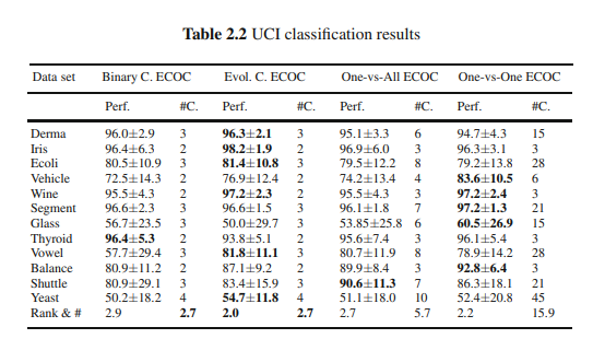
The classification results obtained for all the UCI data sets considering the different ECOC configurations are shown in Table 2.2. In order to compare the performances provided for each strategy, the table also shows the mean rank of each ECOC design considering the twelve different experiments. The rankings are obtained estimating each particular ranking $r_i^j$ for each problem $i$ and each ECOC configuration $j$, and computing the mean ranking $R$ for each design as $R_j=\frac{1}{N} \sum_i r_i^j$, where $N$ is the total number of data sets. We also show the mean number of classifiers (#) required for each strategy.

In order to analyze if the difference between ranks (and hence, the methods) is statistically significant, we apply a statistical test. In order to reject the null hypothesis (which implies no significant statistical difference among measured ranks and the mean rank), we use the Friedman test. The Friedman statistic value is computed as follows:
$$
X_F^2=\frac{12 N}{k(k+1)}\left[\sum_j R_j^2-\frac{k(k+1)^2}{4}\right] .
$$
In our case, with $k=4$ ECOC designs to compare, $X_F^2=-4.94$. Since this value is rather conservative, Iman and Davenport proposed a corrected statistic:
$$
F_F=\frac{(N-1) X_F^2}{N(k-1)-X_F^2}
$$

Applying this correction we obtain $F_F=-1.32$. With four methods and twelve experiments, $F_F$ is distributed according to the $F$ distribution with 3 and 33 degrees of freedom. The critical value of $F(3,33)$ for 0.05 is 2.89 . As the value of $F_F$ is no higher than 2.98 we can state that there is no statistically significant difference among the ECOC schemes. This means that all four strategies are suitable in order to deal with multi-class categorization problems. This result is very satisfactory and encourages the use of the compact approach since similar (or even better) results can be obtained with far less number of classifiers. Moreover, the GA evolutionary version of the compact design improves in the mean rank to the rest of classical coding strategies, and in most cases outperforms the binary compact approach in the present experiment. This result is expected since the evolutionary version looks for a compact ECOC matrix configuration that minimizes the error over the training data. In particular, the advantage of the evolutionary version over the binary one is more significant when the number of classes increases, since more compact matrices are available for optimization.

计算机代写|机器学习代写machine learning代考|Labelled Faces in the Wild Categorization

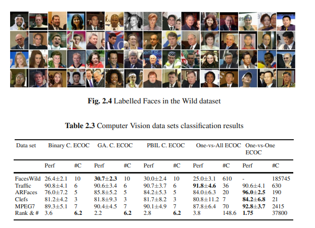
This dataset contains 13000 faces images taken directly from the web from over 1400 people. These images are not constrained in terms of pose, light, occlusions or any other relevant factor. For the purpose of this experiment we used a specific subset, taking only the categories which at least have four or more examples, having a total of 610 face categories. Finally, in order to extract relevant features from the images, we apply an Incremental Principal Component Analysis procedure [16], keeping $99.8 \%$ of the information. An example of face images is shown in Fig. 2.4.
The results in the first row of Table 2.3 show that the best performance is obtained by the Evolutionary GA and PBIL compact strategies. One important observation is that Evolutionary strategies outperform the classical one-versus-all approach, with far less number of classifiers (10 instead of 610). Note that in this case we omitted the one-vs-one strategy since it requires 185745 classifiers for discriminating 610 face categories.

For this second computer vision experiment, we use the video sequences obtained from the Mobile Mapping System of [1] to test the ECOC methodology on a real traffic sign categorization problem. In this system, the position and orientation of the different traffic signs are measured with video cameras fixed on a moving vehicle. The system has a stereo pair of calibrated cameras, which are synchronized with a GPS/INS system. The result of the acquisition step is a set of stereo-pairs of images with their position and orientation information. From this system, a set of 36 circular and triangular traffic sign classes are obtained. Some categories from this data set are shown in Fig. 2.5. The data set contains a total of 3481 samples of size $32 \times 32$, filtered using the Weickert anisotropic filter, masked to exclude the background pixels, and equalized to prevent the effects of illumination changes. These feature vectors are then projected into a 100 feature vector by means of PCA.

The classification results obtained when considering the different ECOC configurations are shown in the second row of Table 2.3. The ECOC designs obtain similar classification results with an accuracy of over $90 \%$. However, note that the compact methodologies use six times less classifiers than the one-versus-all and 105 less times classifiers than the one-versus-one approach, respectively.

计算机代写|机器学习代写machine learning代考|STAT3888

机器学习代考

计算机代写|机器学习代写machine learning代考|UCI Categorization

考虑不同ECOC配置的所有UCI数据集的分类结果如表2.2所示。为了比较每种策略提供的性能,下表还显示了考虑到12种不同实验的每种ECOC设计的平均排名。通过估计每个问题$i$和每个ECOC配置$j$的每个特定排名$r_i^j$得到排名,并计算每个设计的平均排名$R$为$R_j=\frac{1}{N} \sum_i r_i^j$,其中$N$为数据集的总数。我们还展示了每种策略所需的分类器的平均数量(#)。

为了分析等级之间的差异(以及方法之间的差异)是否具有统计显著性,我们应用了统计检验。为了拒绝零假设(这意味着测量秩和平均秩之间没有显著的统计差异),我们使用弗里德曼检验。弗里德曼统计值计算公式如下:
$$
X_F^2=\frac{12 N}{k(k+1)}\left[\sum_j R_j^2-\frac{k(k+1)^2}{4}\right] .
$$
在我们的案例中,与$k=4$ ECOC设计进行比较,$X_F^2=-4.94$。由于这个值相当保守,Iman和Davenport提出了一个修正后的统计:
$$
F_F=\frac{(N-1) X_F^2}{N(k-1)-X_F^2}
$$

应用这个修正,我们得到$F_F=-1.32$。通过4种方法和12个实验,$F_F$按照$F$的3自由度和33自由度分布进行分布。$F(3,33)$对0.05的临界值为2.89。由于$F_F$的值不大于2.98,我们可以认为ECOC方案之间没有统计学上的显著差异。这意味着这四种策略都适用于处理多类分类问题。这个结果非常令人满意,并鼓励使用紧凑方法,因为使用更少的分类器可以获得类似(甚至更好)的结果。此外,遗传进化版本的紧凑设计在平均秩上优于其他经典编码策略,并且在大多数情况下优于本实验中的二进制紧凑方法。这个结果是预期的,因为进化版本寻找一个紧凑的ECOC矩阵配置,使训练数据上的误差最小化。特别是,当类的数量增加时,进化版本相对于二进制版本的优势更加显著,因为可以使用更紧凑的矩阵进行优化。

计算机代写|机器学习代写machine learning代考|Labelled Faces in the Wild Categorization

该数据集包含13000张直接从网络上取自1400多人的人脸图像。这些图像不受姿势、光线、遮挡或任何其他相关因素的限制。为了这个实验的目的,我们使用了一个特定的子集,只取至少有四个或更多例子的类别,总共有610个面部类别。最后,为了从图像中提取相关特征,我们应用增量主成分分析程序[16],保留99.8%的信息。一个人脸图像的例子如图2.4所示。
表2.3第一行的结果表明,进化遗传算法和PBIL压缩策略的性能最好。一个重要的观察结果是,进化策略优于经典的“一对全”方法,它的分类器数量要少得多(10个而不是610个)。注意,在这种情况下,我们省略了一对一策略,因为它需要185745个分类器来区分610个人脸类别。

对于第二个计算机视觉实验,我们使用从[1]的移动地图系统获得的视频序列来测试ECOC方法在实际交通标志分类问题上的应用。在这个系统中,不同的交通标志的位置和方向是通过固定在移动车辆上的摄像机来测量的。该系统有一对立体校准相机,与GPS/INS系统同步。采集步骤的结果是一组具有位置和方向信息的立体图像对。从这个系统中,得到了一组36个圆形和三角形交通标志类。该数据集中的一些类别如图2.5所示。该数据集共包含3481个大小为$32 × 32$的样本,使用Weickert各向异性滤波器进行滤波,屏蔽以排除背景像素,并进行均衡以防止光照变化的影响。然后通过PCA将这些特征向量投影成100个特征向量。

考虑不同ECOC配置得到的分类结果如表2.3第二行所示。ECOC设计获得了类似的分类结果,准确率超过90%。但是,请注意,紧凑方法使用的分类器比单对全方法少6倍,比单对一方法少105倍。

计算机代写|机器学习代写machine learning代考 请认准statistics-lab™

统计代写请认准statistics-lab™. statistics-lab™为您的留学生涯保驾护航。

金融工程代写

金融工程是使用数学技术来解决金融问题。金融工程使用计算机科学、统计学、经济学和应用数学领域的工具和知识来解决当前的金融问题,以及设计新的和创新的金融产品。

非参数统计代写

非参数统计指的是一种统计方法,其中不假设数据来自于由少数参数决定的规定模型;这种模型的例子包括正态分布模型和线性回归模型。

广义线性模型代考

广义线性模型(GLM)归属统计学领域,是一种应用灵活的线性回归模型。该模型允许因变量的偏差分布有除了正态分布之外的其它分布。

术语 广义线性模型(GLM)通常是指给定连续和/或分类预测因素的连续响应变量的常规线性回归模型。它包括多元线性回归,以及方差分析和方差分析(仅含固定效应)。

有限元方法代写

有限元方法(FEM)是一种流行的方法,用于数值解决工程和数学建模中出现的微分方程。典型的问题领域包括结构分析、传热、流体流动、质量运输和电磁势等传统领域。

有限元是一种通用的数值方法,用于解决两个或三个空间变量的偏微分方程(即一些边界值问题)。为了解决一个问题,有限元将一个大系统细分为更小、更简单的部分,称为有限元。这是通过在空间维度上的特定空间离散化来实现的,它是通过构建对象的网格来实现的:用于求解的数值域,它有有限数量的点。边界值问题的有限元方法表述最终导致一个代数方程组。该方法在域上对未知函数进行逼近。[1] 然后将模拟这些有限元的简单方程组合成一个更大的方程系统,以模拟整个问题。然后,有限元通过变化微积分使相关的误差函数最小化来逼近一个解决方案。

tatistics-lab作为专业的留学生服务机构,多年来已为美国、英国、加拿大、澳洲等留学热门地的学生提供专业的学术服务,包括但不限于Essay代写,Assignment代写,Dissertation代写,Report代写,小组作业代写,Proposal代写,Paper代写,Presentation代写,计算机作业代写,论文修改和润色,网课代做,exam代考等等。写作范围涵盖高中,本科,研究生等海外留学全阶段,辐射金融,经济学,会计学,审计学,管理学等全球99%专业科目。写作团队既有专业英语母语作者,也有海外名校硕博留学生,每位写作老师都拥有过硬的语言能力,专业的学科背景和学术写作经验。我们承诺100%原创,100%专业,100%准时,100%满意。

随机分析代写


随机微积分是数学的一个分支,对随机过程进行操作。它允许为随机过程的积分定义一个关于随机过程的一致的积分理论。这个领域是由日本数学家伊藤清在第二次世界大战期间创建并开始的。

时间序列分析代写

随机过程,是依赖于参数的一组随机变量的全体,参数通常是时间。 随机变量是随机现象的数量表现,其时间序列是一组按照时间发生先后顺序进行排列的数据点序列。通常一组时间序列的时间间隔为一恒定值(如1秒,5分钟,12小时,7天,1年),因此时间序列可以作为离散时间数据进行分析处理。研究时间序列数据的意义在于现实中,往往需要研究某个事物其随时间发展变化的规律。这就需要通过研究该事物过去发展的历史记录,以得到其自身发展的规律。

回归分析代写

多元回归分析渐进(Multiple Regression Analysis Asymptotics)属于计量经济学领域,主要是一种数学上的统计分析方法,可以分析复杂情况下各影响因素的数学关系,在自然科学、社会和经济学等多个领域内应用广泛。

MATLAB代写

MATLAB 是一种用于技术计算的高性能语言。它将计算、可视化和编程集成在一个易于使用的环境中,其中问题和解决方案以熟悉的数学符号表示。典型用途包括:数学和计算算法开发建模、仿真和原型制作数据分析、探索和可视化科学和工程图形应用程序开发,包括图形用户界面构建MATLAB 是一个交互式系统,其基本数据元素是一个不需要维度的数组。这使您可以解决许多技术计算问题,尤其是那些具有矩阵和向量公式的问题,而只需用 C 或 Fortran 等标量非交互式语言编写程序所需的时间的一小部分。MATLAB 名称代表矩阵实验室。MATLAB 最初的编写目的是提供对由 LINPACK 和 EISPACK 项目开发的矩阵软件的轻松访问,这两个项目共同代表了矩阵计算软件的最新技术。MATLAB 经过多年的发展,得到了许多用户的投入。在大学环境中,它是数学、工程和科学入门和高级课程的标准教学工具。在工业领域,MATLAB 是高效研究、开发和分析的首选工具。MATLAB 具有一系列称为工具箱的特定于应用程序的解决方案。对于大多数 MATLAB 用户来说非常重要,工具箱允许您学习应用专业技术。工具箱是 MATLAB 函数(M 文件)的综合集合,可扩展 MATLAB 环境以解决特定类别的问题。可用工具箱的领域包括信号处理、控制系统、神经网络、模糊逻辑、小波、仿真等。

R语言代写问卷设计与分析代写
PYTHON代写回归分析与线性模型代写
MATLAB代写方差分析与试验设计代写
STATA代写机器学习/统计学习代写
SPSS代写计量经济学代写
EVIEWS代写时间序列分析代写
EXCEL代写深度学习代写
SQL代写各种数据建模与可视化代写

计算机代写|机器学习代写machine learning代考|QBUS3820

如果你也在 怎样代写机器学习Machine Learning 这个学科遇到相关的难题,请随时右上角联系我们的24/7代写客服。机器学习Machine Learning令人兴奋。这是有趣的,具有挑战性的,创造性的,和智力刺激。它还为公司赚钱,自主处理大量任务,并从那些宁愿做其他事情的人那里消除单调工作的繁重任务。

机器学习Machine Learning也非常复杂。从数千种算法、数百种开放源码包,以及需要具备从数据工程(DE)到高级统计分析和可视化等各种技能的专业实践者,ML专业实践者所需的工作确实令人生畏。增加这种复杂性的是,需要能够与广泛的专家、主题专家(sme)和业务单元组进行跨功能工作——就正在解决的问题的性质和ml支持的解决方案的输出进行沟通和协作。

statistics-lab™ 为您的留学生涯保驾护航 在代写机器学习 machine learning方面已经树立了自己的口碑, 保证靠谱, 高质且原创的统计Statistics代写服务。我们的专家在代写机器学习 machine learning代写方面经验极为丰富,各种代写机器学习 machine learning相关的作业也就用不着说。

计算机代写|机器学习代写machine learning代考|QBUS3820

计算机代写|机器学习代写machine learning代考|Evolutionary Compact Parametrization

When defining a compact design of an ECOC, the possible loss of generalization performance has to be taken into account. In order to deal with this problem an evolutionary optimization process is used to find a compact ECOC with high generalization capability.

In order to show the parametrization complexity of the compact ECOC design, we first provide an estimation of the number of different possible ECOC matrices that we can build, and therefore, the search space cardinality. We approximate this number using some simple combinatorial principles. First of all, if we have an $N$-class problem and $B$ possible bits to represent all the classes, we have a set $C W$ with $2^B$ different words. In order to build an ECOC matrix, we select $N$ codewords from $C W$ without replacement. In combinatorics this is represented as $\left(\begin{array}{c}2_N^B \ N\end{array}\right)$, which means that we can construct $V_{2^B}^N=\frac{2^{B} !}{\left(2^B-N\right) !}$ different ECOC matrices. Nevertheless, in the ECOC framework, one matrix and its opposite (swapping all zeros by ones and vice-versa) are considered as the same matrix, since both represent the same partitions of the data. Therefore, the approximated number of possible ECOC matrices with the minimum number of classifiers is $\frac{V_{2 B}^N}{2}=\frac{2^{B} !}{2\left(2^B-N\right) !}$. In addition to the huge cardinality, it is easy to show that this space is neither continuous nor differentiable, because a change in just one bit of the matrix may produce a wrong coding design.

In this type of scenarios, evolutionary approaches are often introduced with good results. Evolutionary algorithms are a wide family of methods that are inspired on the Darwin’s evolution theory, and used to be formulated as optimization processes where the solution space is neither differentiable nor well defined. In these cases, the simulation of natural evolution process using computers results in stochastic optimization techniques which often outperform classical methods of optimization when applied to difficult real-world problems. Although the most used and studied evolutionary algorithms are the Genetic Algorithms (GA), from the publication of the Population Based Incremental Learning (PBIL) in 1995 by Baluja and Caruana [4], a new family of evolutionary methods is striving to find a place in this field. In contrast to $\mathrm{GA}$, those new algorithms consider each value in the chromosome as a random variable, and their goal is to learn a probability model to describe the characteristics of good individuals. In the case of PBIL, if a binary chromosome is used, a uniform distribution is learned in order to estimate the probability of each variable to be one or zero.

In this chapter, we report experiments made with the selected evolutionary strategies – i.e. GA and PBIL. Note that for both Evolutionary Strategies, the encoding step and the adaptation function are exactly equivalent.

计算机代写|机器学习代写machine learning代考|Problem encoding

Problem encoding: The first step in order to use an evolutionary algorithm is to define the problem encoding, which consists of the representation of a certain solution or point in the search space by means of a genotype or alternatively a chromosome [14]. When the solutions or individuals are transformed in order to be represented in a chromosome, the original values (the individuals) are referred as phenotypes, and each one of the possible settings for a phenotype is the allele. Binary encoding is the most common, mainly because the first works about GA used this type of encoding. In binary encoding, every chromosome is a string of bits. Although this encoding is often not natural for many problems and sometimes corrections must be performed after crossover and/or mutation, in our case, the chromosomes represent binary ECOC matrices, and therefore, this encoding perfectly adapts to the problem. Each ECOC is encoded as a binary chromosome $\zeta=$, where $h_i^{c_j} \in{0,1}$ is the expected value of the $i$-th classifier for the class $c_j$, which corresponds to the $i-t h$ bit of the class $c_j$ codeword.

Adaptation function: Once the encoding is defined, we need to define the adaptation function, which associates to each individual its adaptation value to the environment, and thus, their survival probability. In the case of the ECOC framework, the adaptation value must be related to the classification error.

Given a chromosome $\zeta=\left\langle\zeta_0, \zeta_1, \ldots, \zeta_L>\right.$ with $\zeta_i \in{0,1}$, the first step is to recover the ECOC matrix $M$ codified in this chromosome. The elements of $M$ allow to create binary classification problems from the original multi-class problem, following the partitions defined by the ECOC columns. Each binary problem is addressed by means of a binary classifier, which is trained in order to separate both partitions of classes. Assuming that there exists a function $y=f(x)$ that maps each sample $x$ to its real label $y$, training a classifier consists of finding the best parameters $w^$ of a certain function $y=f^{\prime}(x, w)$, in the manner that for any other $w \neq w^, f^{\prime}\left(x, w^\right)$ is a better approximation to $f$ than $f^{\prime}(x, w)$. Once the $w^$ are estimated for each binary problem, the adaptation value corresponds to the classification error. In order to take into account the generalization power of the trained classifiers, the estimation of $w^*$ is performed over a subset of the samples, while the rest of the samples are reserved for a validation set, and the adaptation value $\xi$ is the classification error over that validation subset. The adaptation value for an individual represented by a certain chromosome $\zeta_i$ can be formulated as:
$$
\varepsilon_i\left(P, Y, M_i\right)=\frac{\sum_{j=1}^s \delta\left(\rho_j, M_i\right) \neq y_j}{s},
$$
where $M_i$ is the ECOC matrix encoded in $\zeta_i, P=\left\langle\rho_1, \ldots, \rho_s\right\rangle$ a set of samples, $Y=\left\langle y_1, \ldots, y_s\right\rangle$ the expected labels for samples in $P$, and $\delta$ is the function that returns the classification label applying the decoding strategy.

计算机代写|机器学习代写machine learning代考|QBUS3820

机器学习代考

计算机代写|机器学习代写machine learning代考|Evolutionary Compact Parametrization

在定义ECOC的紧凑设计时,必须考虑到可能的泛化性能损失。为了解决这一问题,采用进化优化方法寻找具有高泛化能力的紧凑ECOC。

为了显示紧凑ECOC设计的参数化复杂性,我们首先提供了我们可以构建的不同可能ECOC矩阵的数量的估计,从而提供了搜索空间基数。我们用一些简单的组合原理来近似这个数字。首先,如果我们有一个$N$ -class问题,并且有$B$个可能的位来表示所有的class,那么我们就有一个包含$2^B$个不同单词的集合$C W$。为了构建ECOC矩阵,我们从$C W$中选择$N$码字而不进行替换。在组合学中,这表示为$\left(\begin{array}{c}2_N^B \ N\end{array}\right)$,这意味着我们可以构造$V_{2^B}^N=\frac{2^{B} !}{\left(2^B-N\right) !}$不同的ECOC矩阵。然而,在ECOC框架中,一个矩阵和它的对立面(用1交换所有零,反之亦然)被认为是相同的矩阵,因为两者都表示数据的相同分区。因此,具有最小分类器数的可能ECOC矩阵的近似值为$\frac{V_{2 B}^N}{2}=\frac{2^{B} !}{2\left(2^B-N\right) !}$。除了巨大的基数之外,很容易表明这个空间既不是连续的也不是可微的,因为仅仅改变矩阵的一位就可能产生错误的编码设计。

在这种类型的场景中,引入进化方法通常会带来良好的结果。进化算法是受达尔文进化论启发的一大类方法,过去常被表述为求解空间既不可微也不能很好定义的优化过程。在这些情况下,使用计算机模拟自然进化过程的结果是随机优化技术,当应用于困难的现实世界问题时,这种技术通常优于经典的优化方法。虽然使用和研究最多的进化算法是遗传算法(Genetic algorithms, GA),但从1995年Baluja和Caruana[4]发表的基于种群的增量学习(Population Based Incremental Learning, PBIL)开始,一个新的进化方法家族正在努力在这一领域找到一席之地。与$\mathrm{GA}$相比,这些新算法将染色体中的每个值视为随机变量,其目标是学习一个概率模型来描述优秀个体的特征。在PBIL的情况下,如果使用双染色体,则学习均匀分布以估计每个变量为1或0的概率。

在本章中,我们报告了用选择的进化策略-即GA和PBIL进行的实验。注意,对于两种进化策略,编码步骤和适应函数是完全相同的。

计算机代写|机器学习代写machine learning代考|Problem encoding

问题编码:使用进化算法的第一步是定义问题编码,问题编码包括通过基因型或染色体在搜索空间中表示某个解或点[14]。当溶液或个体被转化以在染色体中表示时,原始值(个体)被称为表型,而表型的每个可能设置都是等位基因。二进制编码是最常见的,主要是因为关于GA的第一个作品使用了这种类型的编码。在二进制编码中,每条染色体都是一串比特。虽然这种编码对于许多问题来说往往是不自然的,有时在交叉和/或突变之后必须进行修正,但在我们的例子中,染色体代表二进制ECOC矩阵,因此,这种编码完美地适应了问题。每个ECOC被编码为一个二进制染色体$\zeta=$,其中$h_i^{c_j} \in{0,1}$是类$c_j$的$i$ -第一个分类器的期望值,它对应于类$c_j$码字的$i-t h$位。

适应函数:一旦编码被定义,我们需要定义适应函数,它与每个个体对环境的适应值相关联,从而与他们的生存概率相关联。对于ECOC框架,自适应值必须与分类误差相关。

给定一条含有$\zeta_i \in{0,1}$的染色体$\zeta=\left\langle\zeta_0, \zeta_1, \ldots, \zeta_L>\right.$,第一步是恢复在该染色体中编码的ECOC矩阵$M$。$M$的元素允许根据ECOC列定义的分区,从原始的多类问题创建二元分类问题。每个二进制问题都是通过一个二进制分类器来解决的,该分类器是为了分离类的两个分区而训练的。假设存在一个函数$y=f(x)$,它将每个样本$x$映射到它的真实标签$y$,那么训练一个分类器就是找到某个函数$y=f^{\prime}(x, w)$的最佳参数$w^$,因为对于任何其他的$w \neq w^, f^{\prime}\left(x, w^\right)$都比$f^{\prime}(x, w)$更接近$f$。一旦对每个二值问题估计出$w^$,其自适应值就对应于分类误差。为了考虑训练的分类器的泛化能力,对样本的一个子集执行$w^*$的估计,而其余的样本保留给一个验证集,并且自适应值$\xi$是该验证子集上的分类误差。以某条染色体$\zeta_i$为代表的个体的适应值可表示为:
$$
\varepsilon_i\left(P, Y, M_i\right)=\frac{\sum_{j=1}^s \delta\left(\rho_j, M_i\right) \neq y_j}{s},
$$
其中$M_i$是在$\zeta_i, P=\left\langle\rho_1, \ldots, \rho_s\right\rangle$中编码的ECOC矩阵(一组样本),$Y=\left\langle y_1, \ldots, y_s\right\rangle$是$P$中样本的期望标签,$\delta$是应用解码策略返回分类标签的函数。

计算机代写|机器学习代写machine learning代考 请认准statistics-lab™

统计代写请认准statistics-lab™. statistics-lab™为您的留学生涯保驾护航。

金融工程代写

金融工程是使用数学技术来解决金融问题。金融工程使用计算机科学、统计学、经济学和应用数学领域的工具和知识来解决当前的金融问题,以及设计新的和创新的金融产品。

非参数统计代写

非参数统计指的是一种统计方法,其中不假设数据来自于由少数参数决定的规定模型;这种模型的例子包括正态分布模型和线性回归模型。

广义线性模型代考

广义线性模型(GLM)归属统计学领域,是一种应用灵活的线性回归模型。该模型允许因变量的偏差分布有除了正态分布之外的其它分布。

术语 广义线性模型(GLM)通常是指给定连续和/或分类预测因素的连续响应变量的常规线性回归模型。它包括多元线性回归,以及方差分析和方差分析(仅含固定效应)。

有限元方法代写

有限元方法(FEM)是一种流行的方法,用于数值解决工程和数学建模中出现的微分方程。典型的问题领域包括结构分析、传热、流体流动、质量运输和电磁势等传统领域。

有限元是一种通用的数值方法,用于解决两个或三个空间变量的偏微分方程(即一些边界值问题)。为了解决一个问题,有限元将一个大系统细分为更小、更简单的部分,称为有限元。这是通过在空间维度上的特定空间离散化来实现的,它是通过构建对象的网格来实现的:用于求解的数值域,它有有限数量的点。边界值问题的有限元方法表述最终导致一个代数方程组。该方法在域上对未知函数进行逼近。[1] 然后将模拟这些有限元的简单方程组合成一个更大的方程系统,以模拟整个问题。然后,有限元通过变化微积分使相关的误差函数最小化来逼近一个解决方案。

tatistics-lab作为专业的留学生服务机构,多年来已为美国、英国、加拿大、澳洲等留学热门地的学生提供专业的学术服务,包括但不限于Essay代写,Assignment代写,Dissertation代写,Report代写,小组作业代写,Proposal代写,Paper代写,Presentation代写,计算机作业代写,论文修改和润色,网课代做,exam代考等等。写作范围涵盖高中,本科,研究生等海外留学全阶段,辐射金融,经济学,会计学,审计学,管理学等全球99%专业科目。写作团队既有专业英语母语作者,也有海外名校硕博留学生,每位写作老师都拥有过硬的语言能力,专业的学科背景和学术写作经验。我们承诺100%原创,100%专业,100%准时,100%满意。

随机分析代写


随机微积分是数学的一个分支,对随机过程进行操作。它允许为随机过程的积分定义一个关于随机过程的一致的积分理论。这个领域是由日本数学家伊藤清在第二次世界大战期间创建并开始的。

时间序列分析代写

随机过程,是依赖于参数的一组随机变量的全体,参数通常是时间。 随机变量是随机现象的数量表现,其时间序列是一组按照时间发生先后顺序进行排列的数据点序列。通常一组时间序列的时间间隔为一恒定值(如1秒,5分钟,12小时,7天,1年),因此时间序列可以作为离散时间数据进行分析处理。研究时间序列数据的意义在于现实中,往往需要研究某个事物其随时间发展变化的规律。这就需要通过研究该事物过去发展的历史记录,以得到其自身发展的规律。

回归分析代写

多元回归分析渐进(Multiple Regression Analysis Asymptotics)属于计量经济学领域,主要是一种数学上的统计分析方法,可以分析复杂情况下各影响因素的数学关系,在自然科学、社会和经济学等多个领域内应用广泛。

MATLAB代写

MATLAB 是一种用于技术计算的高性能语言。它将计算、可视化和编程集成在一个易于使用的环境中,其中问题和解决方案以熟悉的数学符号表示。典型用途包括:数学和计算算法开发建模、仿真和原型制作数据分析、探索和可视化科学和工程图形应用程序开发,包括图形用户界面构建MATLAB 是一个交互式系统,其基本数据元素是一个不需要维度的数组。这使您可以解决许多技术计算问题,尤其是那些具有矩阵和向量公式的问题,而只需用 C 或 Fortran 等标量非交互式语言编写程序所需的时间的一小部分。MATLAB 名称代表矩阵实验室。MATLAB 最初的编写目的是提供对由 LINPACK 和 EISPACK 项目开发的矩阵软件的轻松访问,这两个项目共同代表了矩阵计算软件的最新技术。MATLAB 经过多年的发展,得到了许多用户的投入。在大学环境中,它是数学、工程和科学入门和高级课程的标准教学工具。在工业领域,MATLAB 是高效研究、开发和分析的首选工具。MATLAB 具有一系列称为工具箱的特定于应用程序的解决方案。对于大多数 MATLAB 用户来说非常重要,工具箱允许您学习应用专业技术。工具箱是 MATLAB 函数(M 文件)的综合集合,可扩展 MATLAB 环境以解决特定类别的问题。可用工具箱的领域包括信号处理、控制系统、神经网络、模糊逻辑、小波、仿真等。

R语言代写问卷设计与分析代写
PYTHON代写回归分析与线性模型代写
MATLAB代写方差分析与试验设计代写
STATA代写机器学习/统计学习代写
SPSS代写计量经济学代写
EVIEWS代写时间序列分析代写
EXCEL代写深度学习代写
SQL代写各种数据建模与可视化代写

计算机代写|机器学习代写machine learning代考|MKTG6010

如果你也在 怎样代写机器学习Machine Learning 这个学科遇到相关的难题,请随时右上角联系我们的24/7代写客服。机器学习Machine Learning令人兴奋。这是有趣的,具有挑战性的,创造性的,和智力刺激。它还为公司赚钱,自主处理大量任务,并从那些宁愿做其他事情的人那里消除单调工作的繁重任务。

机器学习Machine Learning也非常复杂。从数千种算法、数百种开放源码包,以及需要具备从数据工程(DE)到高级统计分析和可视化等各种技能的专业实践者,ML专业实践者所需的工作确实令人生畏。增加这种复杂性的是,需要能够与广泛的专家、主题专家(sme)和业务单元组进行跨功能工作——就正在解决的问题的性质和ml支持的解决方案的输出进行沟通和协作。

statistics-lab™ 为您的留学生涯保驾护航 在代写机器学习 machine learning方面已经树立了自己的口碑, 保证靠谱, 高质且原创的统计Statistics代写服务。我们的专家在代写机器学习 machine learning代写方面经验极为丰富,各种代写机器学习 machine learning相关的作业也就用不着说。

计算机代写|机器学习代写machine learning代考|MKTG6010

计算机代写|机器学习代写machine learning代考|Local Binary Patterns

The local binary pattern (LBP) operator [14] is a powerful $2 \mathrm{D}$ texture descriptor that has the benefit of being somewhat insensitive to variations in the lighting and orientation of an image. The method has been successfully applied to applications such as face recognition [1] and facial expression recognition [16]. As illustrated in Fig. 1.2, the LBP algorithm associates each interior pixel of an intensity image with a binary code number in the range $0-256$. This code number is generated by taking the surrounding pixels and, working in a clockwise direction from the top left hand corner, assigning a bit value of 0 where the neighbouring pixel intensity is less than that of the central pixel and 1 otherwise. The concatenation of these bits produces an eight-digit binary code word which becomes the grey-scale value of the corresponding pixel in the transformed image. Figure 1.2 shows a pixel being compared with its immediate neighbours. It is however also possible to compare a pixel with others which are separated by distances of two, three or more pixel widths, giving rise to a series of transformed images. Each such image is generated using a different radius for the circularly symmetric neighbourhood over which the LBP code is calculated.

Another possible refinement is to obtain a finer angular resolution by using more than 8 bits in the code-word [14]. Note that the choice of the top left hand corner as a reference point is arbitrary and that different choices would lead to different LBP codes; valid comparisons can be made, however, provided that the same choice of reference point is made for all pixels in all images.

It is noted in [14] that in practice the majority of LBP codes consist of a concatenation of at most three consecutive sub-strings of $0 \mathrm{~s}$ and $1 \mathrm{~s}$; this means that when the circular neighbourhood of the centre pixel is traversed, the result is either all $0 \mathrm{~s}$, all $1 \mathrm{~s}$ or a starting point can be found which produces a sequence of 0 s followed by a sequence of $1 \mathrm{~s}$. These codes are referred to as uniform patterns and, for an 8 bit code, there are 58 possible values. Uniform patterns are most useful for texture discrimination purposes as they represent local micro-features such as bright spots, flat spots and edges; non-uniform patterns tend to be a source of noise and can therefore usefully be mapped to the single common value 59 .

In order to use LBP codes as a face expression comparison mechanism it is first necessary to subdivide a face image into a number of sub-windows and then compute the occurrence histograms of the LBP codes over these regions. These histograms can be combined to generate useful features, for example by concatenating them or by comparing corresponding histograms from two images.

计算机代写|机器学习代写machine learning代考|Fast Correlation-Based Filtering

Broadly speaking, feature selection algorithms can be divided into two groups: wrapper methods and filter methods [3]. In the wrapper approach different combinations of features are considered and a classifier is trained on each combination to determine which is the most effective. Whilst this approach undoubtedly gives good results, the computational demands that it imposes render it impractical when a very large number of features needs to be considered. In such cases the filter approach may be used; this considers the merits of features in themselves without reference to any particular classification method.

Fast correlation-based filtering (FCBF) has proved itself to be a successful feature selection method that can handle large numbers of features in a computationally efficient way. It works by considering the classification between each feature and the class label and between each pair of features. As a measure of classification the concept of symmetric uncertainty is used; for a pair random variables $X$ and $Y$ this is defined as:
$$
S U(X, Y)=2\left[\frac{I G(X, Y)}{H(X)+H(Y)}\right]
$$
where $H(\cdot)$ is the entropy of the random variable and $I G(X, Y)=H(X)-H(X \mid Y)=$ $H(Y)-H(Y \mid X)$ is the information gain between $X$ and $Y$. As its name suggests, symmetric uncertainty is symmetric in its arguments; it takes values in the range $[0,1]$ where 0 implies independence between the random variables and 1 implies that the value of each variable completely predicts the value of the other. In calculating the entropies of Eq. 1.6, any continuous features must first be discretised.

The FCBF algorithm applies heuristic principles that aim to achieve a balance between using relevant features and avoiding redundant features. It does this by selecting features $f$ that satisfy the following properties:

  1. $S U(f, c) \geq \delta$ where $c$ is the class label and $\delta$ is a threshold value chosen to suit the application.
  2. $\forall g: S U(f, g) \geq S U(f, c) \Rightarrow S U(f, c) \geq S U(g, c)$ where $g$ is any feature other than $f$.

Here, property 1 ensures that the selected features are relevant, in that they are correlated with the class label to some degree, and property 2 eliminates redundant features by discarding those that are strongly correlated with a more relevant feature.

计算机代写|机器学习代写machine learning代考|MKTG6010

机器学习代考

计算机代写|机器学习代写machine learning代考|Local Binary Patterns

局部二元模式(LBP)算子[14]是一种功能强大的$2 \mathrm{D}$纹理描述符,其优点是对图像的光照和方向变化不敏感。该方法已成功应用于人脸识别[1]、面部表情识别[16]等应用。如图1.2所示,LBP算法将强度图像的每个内部像素与范围为$0-256$的二进制码数相关联。这个代码号是通过取周围的像素,从左上角开始顺时针方向工作,在邻近像素强度小于中心像素时分配位值0,否则分配位值1来生成的。这些位的连接产生一个8位二进制码字,它成为转换后的图像中相应像素的灰度值。图1.2显示了一个像素与其近邻的比较。然而,也可以将一个像素与被两个、三个或更多像素宽度的距离隔开的其他像素进行比较,从而产生一系列转换后的图像。每个这样的图像都是使用不同半径的圆对称邻域来生成的,LBP代码是在这个邻域上计算的。

另一种可能的改进是通过在码字中使用超过8位来获得更精细的角度分辨率[14]。注意,左上角作为参考点的选择是任意的,不同的选择将导致不同的LBP代码;然而,只要对所有图像中的所有像素选择相同的参考点,就可以进行有效的比较。

在[14]中指出,在实践中,大多数LBP码由最多三个连续的$0 \mathrm{~s}$和$1 \mathrm{~s}$子串组成;这意味着当遍历中心像素的圆形邻域时,结果要么是全部$0 \mathrm{~s}$,全部$1 \mathrm{~s}$,要么可以找到一个起点,它产生一个0 s序列,后面是一个$1 \mathrm{~s}$序列。这些代码被称为统一模式,对于一个8位的代码,有58个可能的值。均匀的图案在纹理识别中最有用,因为它们代表了局部的微特征,如亮点、平斑和边缘;不均匀的模式往往是噪声源,因此可以有效地映射到单一的公共值59。

为了使用LBP码作为人脸表情比较机制,首先需要将人脸图像细分为多个子窗口,然后计算这些区域上LBP码的出现直方图。这些直方图可以组合起来生成有用的特征,例如通过连接它们或比较来自两幅图像的相应直方图。

计算机代写|机器学习代写machine learning代考|Fast Correlation-Based Filtering

包装器方法考虑了不同的特征组合,并在每种组合上训练分类器,以确定哪种组合最有效。虽然这种方法无疑给出了很好的结果,但当需要考虑非常大量的特征时,它所施加的计算需求使其不切实际。在这种情况下,可以使用过滤器方法;这考虑了特征本身的优点,而不参考任何特定的分类方法。

快速相关滤波(Fast correlation-based filtering, FCBF)是一种成功的特征选择方法,能够以高效的计算方式处理大量特征。它通过考虑每个特征与类标号之间以及每对特征之间的分类来工作。作为分类的度量,对称不确定性的概念被使用;对于一对随机变量$X$和$Y$,定义为:
$$
S U(X, Y)=2\left[\frac{I G(X, Y)}{H(X)+H(Y)}\right]
$$
其中$H(\cdot)$为随机变量的熵,$I G(X, Y)=H(X)-H(X \mid Y)=$$H(Y)-H(Y \mid X)$为$X$与$Y$之间的信息增益。顾名思义,对称不确定性在其参数中是对称的;它的取值范围为$[0,1]$,其中0表示随机变量之间的独立性,1表示每个变量的值完全预测另一个变量的值。在计算Eq. 1.6的熵时,必须首先对任何连续特征进行离散。

FCBF算法采用启发式原则,目的是在使用相关特征和避免冗余特征之间取得平衡。它通过选择满足以下属性的功能$f$来实现这一点:

$S U(f, c) \geq \delta$ 其中$c$是类标签,$\delta$是为适应应用程序而选择的阈值。

$\forall g: S U(f, g) \geq S U(f, c) \Rightarrow S U(f, c) \geq S U(g, c)$ 其中$g$是除$f$之外的任何特性。

在这里,属性1确保所选择的特征是相关的,因为它们在某种程度上与类标签相关,而属性2通过丢弃那些与更相关的特征强烈相关的特征来消除冗余特征

计算机代写|机器学习代写machine learning代考 请认准statistics-lab™

统计代写请认准statistics-lab™. statistics-lab™为您的留学生涯保驾护航。

金融工程代写

金融工程是使用数学技术来解决金融问题。金融工程使用计算机科学、统计学、经济学和应用数学领域的工具和知识来解决当前的金融问题,以及设计新的和创新的金融产品。

非参数统计代写

非参数统计指的是一种统计方法,其中不假设数据来自于由少数参数决定的规定模型;这种模型的例子包括正态分布模型和线性回归模型。

广义线性模型代考

广义线性模型(GLM)归属统计学领域,是一种应用灵活的线性回归模型。该模型允许因变量的偏差分布有除了正态分布之外的其它分布。

术语 广义线性模型(GLM)通常是指给定连续和/或分类预测因素的连续响应变量的常规线性回归模型。它包括多元线性回归,以及方差分析和方差分析(仅含固定效应)。

有限元方法代写

有限元方法(FEM)是一种流行的方法,用于数值解决工程和数学建模中出现的微分方程。典型的问题领域包括结构分析、传热、流体流动、质量运输和电磁势等传统领域。

有限元是一种通用的数值方法,用于解决两个或三个空间变量的偏微分方程(即一些边界值问题)。为了解决一个问题,有限元将一个大系统细分为更小、更简单的部分,称为有限元。这是通过在空间维度上的特定空间离散化来实现的,它是通过构建对象的网格来实现的:用于求解的数值域,它有有限数量的点。边界值问题的有限元方法表述最终导致一个代数方程组。该方法在域上对未知函数进行逼近。[1] 然后将模拟这些有限元的简单方程组合成一个更大的方程系统,以模拟整个问题。然后,有限元通过变化微积分使相关的误差函数最小化来逼近一个解决方案。

tatistics-lab作为专业的留学生服务机构,多年来已为美国、英国、加拿大、澳洲等留学热门地的学生提供专业的学术服务,包括但不限于Essay代写,Assignment代写,Dissertation代写,Report代写,小组作业代写,Proposal代写,Paper代写,Presentation代写,计算机作业代写,论文修改和润色,网课代做,exam代考等等。写作范围涵盖高中,本科,研究生等海外留学全阶段,辐射金融,经济学,会计学,审计学,管理学等全球99%专业科目。写作团队既有专业英语母语作者,也有海外名校硕博留学生,每位写作老师都拥有过硬的语言能力,专业的学科背景和学术写作经验。我们承诺100%原创,100%专业,100%准时,100%满意。

随机分析代写


随机微积分是数学的一个分支,对随机过程进行操作。它允许为随机过程的积分定义一个关于随机过程的一致的积分理论。这个领域是由日本数学家伊藤清在第二次世界大战期间创建并开始的。

时间序列分析代写

随机过程,是依赖于参数的一组随机变量的全体,参数通常是时间。 随机变量是随机现象的数量表现,其时间序列是一组按照时间发生先后顺序进行排列的数据点序列。通常一组时间序列的时间间隔为一恒定值(如1秒,5分钟,12小时,7天,1年),因此时间序列可以作为离散时间数据进行分析处理。研究时间序列数据的意义在于现实中,往往需要研究某个事物其随时间发展变化的规律。这就需要通过研究该事物过去发展的历史记录,以得到其自身发展的规律。

回归分析代写

多元回归分析渐进(Multiple Regression Analysis Asymptotics)属于计量经济学领域,主要是一种数学上的统计分析方法,可以分析复杂情况下各影响因素的数学关系,在自然科学、社会和经济学等多个领域内应用广泛。

MATLAB代写

MATLAB 是一种用于技术计算的高性能语言。它将计算、可视化和编程集成在一个易于使用的环境中,其中问题和解决方案以熟悉的数学符号表示。典型用途包括:数学和计算算法开发建模、仿真和原型制作数据分析、探索和可视化科学和工程图形应用程序开发,包括图形用户界面构建MATLAB 是一个交互式系统,其基本数据元素是一个不需要维度的数组。这使您可以解决许多技术计算问题,尤其是那些具有矩阵和向量公式的问题,而只需用 C 或 Fortran 等标量非交互式语言编写程序所需的时间的一小部分。MATLAB 名称代表矩阵实验室。MATLAB 最初的编写目的是提供对由 LINPACK 和 EISPACK 项目开发的矩阵软件的轻松访问,这两个项目共同代表了矩阵计算软件的最新技术。MATLAB 经过多年的发展,得到了许多用户的投入。在大学环境中,它是数学、工程和科学入门和高级课程的标准教学工具。在工业领域,MATLAB 是高效研究、开发和分析的首选工具。MATLAB 具有一系列称为工具箱的特定于应用程序的解决方案。对于大多数 MATLAB 用户来说非常重要,工具箱允许您学习应用专业技术。工具箱是 MATLAB 函数(M 文件)的综合集合,可扩展 MATLAB 环境以解决特定类别的问题。可用工具箱的领域包括信号处理、控制系统、神经网络、模糊逻辑、小波、仿真等。

R语言代写问卷设计与分析代写
PYTHON代写回归分析与线性模型代写
MATLAB代写方差分析与试验设计代写
STATA代写机器学习/统计学习代写
SPSS代写计量经济学代写
EVIEWS代写时间序列分析代写
EXCEL代写深度学习代写
SQL代写各种数据建模与可视化代写

计算机代写|机器学习代写machine learning代考|COMP4318

如果你也在 怎样代写机器学习Machine Learning 这个学科遇到相关的难题,请随时右上角联系我们的24/7代写客服。机器学习Machine Learning令人兴奋。这是有趣的,具有挑战性的,创造性的,和智力刺激。它还为公司赚钱,自主处理大量任务,并从那些宁愿做其他事情的人那里消除单调工作的繁重任务。

机器学习Machine Learning也非常复杂。从数千种算法、数百种开放源码包,以及需要具备从数据工程(DE)到高级统计分析和可视化等各种技能的专业实践者,ML专业实践者所需的工作确实令人生畏。增加这种复杂性的是,需要能够与广泛的专家、主题专家(sme)和业务单元组进行跨功能工作——就正在解决的问题的性质和ml支持的解决方案的输出进行沟通和协作。

statistics-lab™ 为您的留学生涯保驾护航 在代写机器学习 machine learning方面已经树立了自己的口碑, 保证靠谱, 高质且原创的统计Statistics代写服务。我们的专家在代写机器学习 machine learning代写方面经验极为丰富,各种代写机器学习 machine learning相关的作业也就用不着说。

计算机代写|机器学习代写machine learning代考|COMP4318

计算机代写|机器学习代写machine learning代考|Bulk external delivery

The considerations for bulk external delivery aren’t substantially different from internal use serving to a database or data warehouse. The only material differences between these serving cases are in the realms of delivery time and monitoring of the predictions.
DELIVERY CONSISTENCY
Bulk delivery of results to an external party has the same relevancy requirements as any other ML solution. Whether you’re building something for an internal team or generating predictions that will be end-user-customer facing, the goal of creating useful predictions doesn’t change.

The one thing that does change with providing bulk predictions to an outside organization (generally applicable to business-to-business companies) when compared to other serving paradigms is in the timeliness of the delivery. While it may be obvious that a failure to deliver an extract of bulk predictions entirely is a bad thing, an inconsistent delivery can be just as detrimental. There is a simple solution to this, however, illustrated in the bottom portion of figure 16.14.

Figure 16.14 shows the comparison of gated and ungated serving to an external user group. By controlling a final-stage egress from the stored predictions in a scheduled batch prediction job, as well as coupling feature-generation logic to an ETL process governed by a feature store, delivery consistency from a chronological perspective can be guaranteed. While this may not seem an important consideration from the DS perspective of the team generating the predictions, having a predictable dataavailability schedule can dramatically increase the perceived professionalism of the serving company.

计算机代写|机器学习代写machine learning代考|QUALITY ASSURANCE

An occasionally overlooked aspect of serving bulk predictions externally (external to the DS and analytics groups at a company) is ensuring that a thorough quality check is performed on those predictions.

An internal project may rely on a simple check for overt prediction failures (for example, silent failures are ignored that result in null values, or a linear model predicts infinity). When sending data products externally, additional steps should be done to minimize the chances of end users of predictions finding fault with them. Since we, as humans, are so adept at finding abnormalities in patterns, a few scant issues in a batch-delivered prediction dataset can easily draw the focus of a consumer of the data, deteriorating their faith in the efficacy of the solution to the point of disuse.

In my experience, when delivering bulk predictions external to a team of data specialists, I’ve found it worthwhile to perform a few checks before releasing the data:

  • Validate the predictions against the training data:
  • Classification problems-Comparing aggregated class counts
  • Regression problems-Comparing prediction distribution
  • Unsupervised problems-Evaluating group membership counts
  • Check for prediction outliers (applicable to regression problems).
  • Build (if applicable) heuristics rules based on knowledge from SMEs to ensure that predictions are not outside the realm of possibility for the topic.
  • Validate incoming features (particularly encoded ones that may use a generic catchall encoding if the encoding key is previously unseen) to ensure that the data is fully compatible with the model as it was trained.

By running a few extra validation steps on the output of a batch prediction, a great deal of confusion and potential lessening of trust in the final product can be avoided in the eyes of end users.

计算机代写|机器学习代写machine learning代考|COMP4318

机器学习代考

计算机代写|机器学习代写machine learning代考|Bulk external delivery

批量外部交付的考虑因素与数据库或数据仓库的内部使用没有本质上的区别。这些服务案例之间唯一的实质性区别在于交付时间和预测监控方面。
交付的一致性
将结果批量交付给外部方与任何其他ML解决方案具有相同的相关性要求。无论您是在为内部团队构建某些东西,还是生成面向最终用户-客户的预测,创建有用预测的目标都不会改变。

与其他服务范式相比,向外部组织提供批量预测(通常适用于b2b公司)确实改变了一件事,那就是交付的及时性。虽然很明显,不能完全交付批量预测的摘要是一件坏事,但不一致的交付可能同样有害。但是,有一个简单的解决方案,如图16.14的底部部分所示。

图16.14显示了为外部用户组服务的门控和不门控的比较。通过控制计划批处理预测作业中存储的预测的最后阶段出口,以及将特征生成逻辑耦合到由特征存储管理的ETL过程,可以保证从时间顺序角度来看交付的一致性。虽然从生成预测的团队的DS角度来看,这似乎不是一个重要的考虑因素,但拥有可预测的数据可用性时间表可以显著提高服务公司的专业水平。

计算机代写|机器学习代写machine learning代考|QUALITY ASSURANCE

在向外部(公司的DS和分析组外部)提供批量预测时,一个偶尔被忽视的方面是确保对这些预测执行彻底的质量检查。

内部项目可能依赖于对公开预测失败的简单检查(例如,忽略导致空值的静默失败,或者线性模型预测无穷大)。在向外部发送数据产品时,应该采取额外的步骤,以尽量减少预测的最终用户发现错误的可能性。作为人类,我们非常善于发现模式中的异常,因此批量交付的预测数据集中的一些小问题很容易吸引数据消费者的注意力,从而降低他们对解决方案有效性的信心,直至不再使用。

根据我的经验,当向数据专家团队外部交付批量预测时,我发现在发布数据之前执行一些检查是值得的:

根据训练数据验证预测:

分类问题——比较聚合类计数

回归问题-比较预测分布

不受监督的问题——评估团队成员数量

检查预测异常值(适用于回归问题)。

基于中小企业的知识构建启发式规则(如果适用),以确保预测不会超出主题的可能性范围。

验证传入的特性(特别是编码的特性,如果编码键以前未见过,则可能使用通用的通用编码),以确保数据在训练时与模型完全兼容。

通过在批预测的输出上运行一些额外的验证步骤,可以避免在最终用户眼中对最终产品的大量混淆和潜在的信任度降低。

计算机代写|机器学习代写machine learning代考 请认准statistics-lab™

统计代写请认准statistics-lab™. statistics-lab™为您的留学生涯保驾护航。

金融工程代写

金融工程是使用数学技术来解决金融问题。金融工程使用计算机科学、统计学、经济学和应用数学领域的工具和知识来解决当前的金融问题,以及设计新的和创新的金融产品。

非参数统计代写

非参数统计指的是一种统计方法,其中不假设数据来自于由少数参数决定的规定模型;这种模型的例子包括正态分布模型和线性回归模型。

广义线性模型代考

广义线性模型(GLM)归属统计学领域,是一种应用灵活的线性回归模型。该模型允许因变量的偏差分布有除了正态分布之外的其它分布。

术语 广义线性模型(GLM)通常是指给定连续和/或分类预测因素的连续响应变量的常规线性回归模型。它包括多元线性回归,以及方差分析和方差分析(仅含固定效应)。

有限元方法代写

有限元方法(FEM)是一种流行的方法,用于数值解决工程和数学建模中出现的微分方程。典型的问题领域包括结构分析、传热、流体流动、质量运输和电磁势等传统领域。

有限元是一种通用的数值方法,用于解决两个或三个空间变量的偏微分方程(即一些边界值问题)。为了解决一个问题,有限元将一个大系统细分为更小、更简单的部分,称为有限元。这是通过在空间维度上的特定空间离散化来实现的,它是通过构建对象的网格来实现的:用于求解的数值域,它有有限数量的点。边界值问题的有限元方法表述最终导致一个代数方程组。该方法在域上对未知函数进行逼近。[1] 然后将模拟这些有限元的简单方程组合成一个更大的方程系统,以模拟整个问题。然后,有限元通过变化微积分使相关的误差函数最小化来逼近一个解决方案。

tatistics-lab作为专业的留学生服务机构,多年来已为美国、英国、加拿大、澳洲等留学热门地的学生提供专业的学术服务,包括但不限于Essay代写,Assignment代写,Dissertation代写,Report代写,小组作业代写,Proposal代写,Paper代写,Presentation代写,计算机作业代写,论文修改和润色,网课代做,exam代考等等。写作范围涵盖高中,本科,研究生等海外留学全阶段,辐射金融,经济学,会计学,审计学,管理学等全球99%专业科目。写作团队既有专业英语母语作者,也有海外名校硕博留学生,每位写作老师都拥有过硬的语言能力,专业的学科背景和学术写作经验。我们承诺100%原创,100%专业,100%准时,100%满意。

随机分析代写


随机微积分是数学的一个分支,对随机过程进行操作。它允许为随机过程的积分定义一个关于随机过程的一致的积分理论。这个领域是由日本数学家伊藤清在第二次世界大战期间创建并开始的。

时间序列分析代写

随机过程,是依赖于参数的一组随机变量的全体,参数通常是时间。 随机变量是随机现象的数量表现,其时间序列是一组按照时间发生先后顺序进行排列的数据点序列。通常一组时间序列的时间间隔为一恒定值(如1秒,5分钟,12小时,7天,1年),因此时间序列可以作为离散时间数据进行分析处理。研究时间序列数据的意义在于现实中,往往需要研究某个事物其随时间发展变化的规律。这就需要通过研究该事物过去发展的历史记录,以得到其自身发展的规律。

回归分析代写

多元回归分析渐进(Multiple Regression Analysis Asymptotics)属于计量经济学领域,主要是一种数学上的统计分析方法,可以分析复杂情况下各影响因素的数学关系,在自然科学、社会和经济学等多个领域内应用广泛。

MATLAB代写

MATLAB 是一种用于技术计算的高性能语言。它将计算、可视化和编程集成在一个易于使用的环境中,其中问题和解决方案以熟悉的数学符号表示。典型用途包括:数学和计算算法开发建模、仿真和原型制作数据分析、探索和可视化科学和工程图形应用程序开发,包括图形用户界面构建MATLAB 是一个交互式系统,其基本数据元素是一个不需要维度的数组。这使您可以解决许多技术计算问题,尤其是那些具有矩阵和向量公式的问题,而只需用 C 或 Fortran 等标量非交互式语言编写程序所需的时间的一小部分。MATLAB 名称代表矩阵实验室。MATLAB 最初的编写目的是提供对由 LINPACK 和 EISPACK 项目开发的矩阵软件的轻松访问,这两个项目共同代表了矩阵计算软件的最新技术。MATLAB 经过多年的发展,得到了许多用户的投入。在大学环境中,它是数学、工程和科学入门和高级课程的标准教学工具。在工业领域,MATLAB 是高效研究、开发和分析的首选工具。MATLAB 具有一系列称为工具箱的特定于应用程序的解决方案。对于大多数 MATLAB 用户来说非常重要,工具箱允许您学习应用专业技术。工具箱是 MATLAB 函数(M 文件)的综合集合,可扩展 MATLAB 环境以解决特定类别的问题。可用工具箱的领域包括信号处理、控制系统、神经网络、模糊逻辑、小波、仿真等。

R语言代写问卷设计与分析代写
PYTHON代写回归分析与线性模型代写
MATLAB代写方差分析与试验设计代写
STATA代写机器学习/统计学习代写
SPSS代写计量经济学代写
EVIEWS代写时间序列分析代写
EXCEL代写深度学习代写
SQL代写各种数据建模与可视化代写

计算机代写|机器学习代写machine learning代考|COMP5328

如果你也在 怎样代写机器学习Machine Learning 这个学科遇到相关的难题,请随时右上角联系我们的24/7代写客服。机器学习Machine Learning令人兴奋。这是有趣的,具有挑战性的,创造性的,和智力刺激。它还为公司赚钱,自主处理大量任务,并从那些宁愿做其他事情的人那里消除单调工作的繁重任务。

机器学习Machine Learning也非常复杂。从数千种算法、数百种开放源码包,以及需要具备从数据工程(DE)到高级统计分析和可视化等各种技能的专业实践者,ML专业实践者所需的工作确实令人生畏。增加这种复杂性的是,需要能够与广泛的专家、主题专家(sme)和业务单元组进行跨功能工作——就正在解决的问题的性质和ml支持的解决方案的输出进行沟通和协作。

statistics-lab™ 为您的留学生涯保驾护航 在代写机器学习 machine learning方面已经树立了自己的口碑, 保证靠谱, 高质且原创的统计Statistics代写服务。我们的专家在代写机器学习 machine learning代写方面经验极为丰富,各种代写机器学习 machine learning相关的作业也就用不着说。

计算机代写|机器学习代写machine learning代考|COMP5328

计算机代写|机器学习代写machine learning代考|Biased testing

Internal testing is easy-well, easier than the alternatives. It’s painless (if the model works properly). It’s what we typically think of when we’re qualifying the results of a project. The process typically involves the following:

  • Generating predictions on new (unseen to the modeling process) data
  • Analyzing the distribution and statistical properties of the new predictions
  • Taking random samples of predictions and making qualitative judgments of them
  • Running handcrafted sample data (or their own accounts, if applicable) through the model

The first two elements in this list are valid for qualification of model effectiveness. They are wholly void of bias and should be done. The latter two, on the other hand, are dangerous. The final one is the more dangerous of them.

In our music playlist generator system scenario, let’s say that the DS team members are all fans of classical music. Throughout their qualitative verifications, they’ve been checking to see the relative quality of the playlist generator for the field of music that they are most familiar with: classical music. To perform these validations, they’ve been generating listening history of their favorite pieces, adjusting the implementation to fine-tune the results, and iterating on the validation process.

When they are fully satisfied that the solution works well at identifying a nearly uncanny level of sophistication for capturing thematic and tonally relevant similar pieces of music, they ask a colleague what they think. The results for both the DS team (Ben and Julie) as well as for their data warehouse engineer friend Connor are shown in figure 15.10.

计算机代写|机器学习代写machine learning代考|Dogfooding

A far more thorough approach than Ben and Julie’s first attempt would have been to canvass people at the company. Instead of keeping the evaluation internal to the team, where a limited exposure to genres hampers their ability to qualitatively measure the effectiveness of the project, they could ask for help. They could ask around and see if people at the company might be interested in taking a look at how their own accounts and usage would be impacted by the changes the DS team is introducing. Figure 15.11 illustrates how this could work for this scenario.

Dogfooding, in the broadest sense, is consuming the results of your own product. The term refers to opening up functionality that is being developed so that everyone at a company can use it, find out how to break it, provide feedback on how it’s broken, and collectively work toward building a better product. All of this happens across a broad range of perspectives, drawing on the experience and knowledge of many employees from all departments.

However, as you can see in figure 15.11, the evaluation still contains bias. An internal user who uses the company’s product is likely not a typical user. Depending on their job function, they may be using their account to validate functionality in the product, use it for demonstrations, or simply interact with the product more because of an employee benefit associated with it.

In addition to the potentially spurious information contained within the listen history of employees, the other form of bias is that people like what they like. They also don’t like what they don’t like. Subjective responses to something as emotionally charged as music preferences add an incredible amount of bias due to the nature of being a member of the human race. Knowing that these predictions are based on their listening history and that it is their own company’s product, internal users evaluating their own profiles will generally be more critical than a typical user if they find something that they don’t like (which is a stark contrast to the builder bias that the DS team would experience).

While dogfooding is certainly preferable to evaluating a solution’s quality within the confines of the DS team, it’s still not ideal, mostly because of these inherent biases that exist.

计算机代写|机器学习代写machine learning代考|COMP5328

机器学习代考

计算机代写|机器学习代写machine learning代考|Biased testing

内部测试很容易——好吧,比其他选择更容易。这是无痛的(如果模型工作正常的话)。这是我们在确定项目结果时通常会想到的。这个过程通常包括以下内容:

在新的(建模过程看不到的)数据上生成预测

分析新预测的分布和统计特性

随机抽取预测样本,并对其进行定性判断

通过模型运行手工制作的示例数据(或他们自己的帐户,如果适用的话)

此列表中的前两个元素对于模型有效性的资格是有效的。他们完全没有偏见,应该这样做。另一方面,后两者是危险的。最后一种是更危险的。

在我们的音乐播放列表生成器系统场景中,假设DS团队成员都是古典音乐迷。在他们的定性验证过程中,他们一直在检查他们最熟悉的音乐领域的播放列表生成器的相对质量:古典音乐。为了执行这些验证,他们已经生成了他们最喜欢的片段的收听历史,调整实现以微调结果,并在验证过程中迭代。

当他们完全满意这个解决方案能够很好地识别出一种近乎不可思议的复杂程度,从而捕捉到主题和音调相关的类似音乐片段时,他们就会询问同事自己的看法。DS团队(Ben和Julie)以及他们的数据仓库工程师朋友Connor的结果如图15.10所示。

计算机代写|机器学习代写machine learning代考|Dogfooding

比本和朱莉的第一次尝试更彻底的方法是在公司里游说。与其在团队内部进行评估(游戏邦注:因为对游戏类型的接触有限而阻碍了他们定性地衡量项目的有效性),他们不如寻求帮助。他们可以四处询问,看看公司里的人是否有兴趣看看他们自己的账户和使用情况会受到DS团队引入的变化的影响。图15.11说明了如何在这个场景中工作。

从最广泛的意义上讲,狗食就是食用自己产品的结果。这个术语指的是开放正在开发的功能,以便公司的每个人都可以使用它,找出如何破坏它,提供关于它如何被破坏的反馈,并共同努力构建更好的产品。所有这些都是在广泛的视角下进行的,利用了各个部门许多员工的经验和知识。

然而,如图15.11所示,评估仍然包含偏差。使用公司产品的内部用户可能不是典型的用户。根据他们的工作职能,他们可能会使用他们的帐户来验证产品中的功能,将其用于演示,或者仅仅是因为与产品相关的员工福利而更多地与产品交互。

除了员工的倾听历史中包含的潜在虚假信息外,另一种形式的偏见是人们喜欢他们喜欢的东西。他们也不喜欢他们不喜欢的东西。对于像音乐偏好这样充满情感的事物的主观反应,由于作为人类一员的本质,增加了难以置信的偏见。知道这些预测是基于他们的收听历史,并且这是他们自己公司的产品,如果内部用户发现他们不喜欢的东西,他们评估自己的资料通常会比普通用户更重要(这与DS团队所经历的构建者偏见形成鲜明对比)。

虽然在DS团队的范围内,狗食肯定比评估解决方案的质量更可取,但它仍然不是理想的,主要是因为存在这些固有的偏见。

计算机代写|机器学习代写machine learning代考 请认准statistics-lab™

统计代写请认准statistics-lab™. statistics-lab™为您的留学生涯保驾护航。

金融工程代写

金融工程是使用数学技术来解决金融问题。金融工程使用计算机科学、统计学、经济学和应用数学领域的工具和知识来解决当前的金融问题,以及设计新的和创新的金融产品。

非参数统计代写

非参数统计指的是一种统计方法,其中不假设数据来自于由少数参数决定的规定模型;这种模型的例子包括正态分布模型和线性回归模型。

广义线性模型代考

广义线性模型(GLM)归属统计学领域,是一种应用灵活的线性回归模型。该模型允许因变量的偏差分布有除了正态分布之外的其它分布。

术语 广义线性模型(GLM)通常是指给定连续和/或分类预测因素的连续响应变量的常规线性回归模型。它包括多元线性回归,以及方差分析和方差分析(仅含固定效应)。

有限元方法代写

有限元方法(FEM)是一种流行的方法,用于数值解决工程和数学建模中出现的微分方程。典型的问题领域包括结构分析、传热、流体流动、质量运输和电磁势等传统领域。

有限元是一种通用的数值方法,用于解决两个或三个空间变量的偏微分方程(即一些边界值问题)。为了解决一个问题,有限元将一个大系统细分为更小、更简单的部分,称为有限元。这是通过在空间维度上的特定空间离散化来实现的,它是通过构建对象的网格来实现的:用于求解的数值域,它有有限数量的点。边界值问题的有限元方法表述最终导致一个代数方程组。该方法在域上对未知函数进行逼近。[1] 然后将模拟这些有限元的简单方程组合成一个更大的方程系统,以模拟整个问题。然后,有限元通过变化微积分使相关的误差函数最小化来逼近一个解决方案。

tatistics-lab作为专业的留学生服务机构,多年来已为美国、英国、加拿大、澳洲等留学热门地的学生提供专业的学术服务,包括但不限于Essay代写,Assignment代写,Dissertation代写,Report代写,小组作业代写,Proposal代写,Paper代写,Presentation代写,计算机作业代写,论文修改和润色,网课代做,exam代考等等。写作范围涵盖高中,本科,研究生等海外留学全阶段,辐射金融,经济学,会计学,审计学,管理学等全球99%专业科目。写作团队既有专业英语母语作者,也有海外名校硕博留学生,每位写作老师都拥有过硬的语言能力,专业的学科背景和学术写作经验。我们承诺100%原创,100%专业,100%准时,100%满意。

随机分析代写


随机微积分是数学的一个分支,对随机过程进行操作。它允许为随机过程的积分定义一个关于随机过程的一致的积分理论。这个领域是由日本数学家伊藤清在第二次世界大战期间创建并开始的。

时间序列分析代写

随机过程,是依赖于参数的一组随机变量的全体,参数通常是时间。 随机变量是随机现象的数量表现,其时间序列是一组按照时间发生先后顺序进行排列的数据点序列。通常一组时间序列的时间间隔为一恒定值(如1秒,5分钟,12小时,7天,1年),因此时间序列可以作为离散时间数据进行分析处理。研究时间序列数据的意义在于现实中,往往需要研究某个事物其随时间发展变化的规律。这就需要通过研究该事物过去发展的历史记录,以得到其自身发展的规律。

回归分析代写

多元回归分析渐进(Multiple Regression Analysis Asymptotics)属于计量经济学领域,主要是一种数学上的统计分析方法,可以分析复杂情况下各影响因素的数学关系,在自然科学、社会和经济学等多个领域内应用广泛。

MATLAB代写

MATLAB 是一种用于技术计算的高性能语言。它将计算、可视化和编程集成在一个易于使用的环境中,其中问题和解决方案以熟悉的数学符号表示。典型用途包括:数学和计算算法开发建模、仿真和原型制作数据分析、探索和可视化科学和工程图形应用程序开发,包括图形用户界面构建MATLAB 是一个交互式系统,其基本数据元素是一个不需要维度的数组。这使您可以解决许多技术计算问题,尤其是那些具有矩阵和向量公式的问题,而只需用 C 或 Fortran 等标量非交互式语言编写程序所需的时间的一小部分。MATLAB 名称代表矩阵实验室。MATLAB 最初的编写目的是提供对由 LINPACK 和 EISPACK 项目开发的矩阵软件的轻松访问,这两个项目共同代表了矩阵计算软件的最新技术。MATLAB 经过多年的发展,得到了许多用户的投入。在大学环境中,它是数学、工程和科学入门和高级课程的标准教学工具。在工业领域,MATLAB 是高效研究、开发和分析的首选工具。MATLAB 具有一系列称为工具箱的特定于应用程序的解决方案。对于大多数 MATLAB 用户来说非常重要,工具箱允许您学习应用专业技术。工具箱是 MATLAB 函数(M 文件)的综合集合,可扩展 MATLAB 环境以解决特定类别的问题。可用工具箱的领域包括信号处理、控制系统、神经网络、模糊逻辑、小波、仿真等。

R语言代写问卷设计与分析代写
PYTHON代写回归分析与线性模型代写
MATLAB代写方差分析与试验设计代写
STATA代写机器学习/统计学习代写
SPSS代写计量经济学代写
EVIEWS代写时间序列分析代写
EXCEL代写深度学习代写
SQL代写各种数据建模与可视化代写

计算机代写|机器学习代写machine learning代考|COMP5318

如果你也在 怎样代写机器学习Machine Learning 这个学科遇到相关的难题,请随时右上角联系我们的24/7代写客服。机器学习Machine Learning令人兴奋。这是有趣的,具有挑战性的,创造性的,和智力刺激。它还为公司赚钱,自主处理大量任务,并从那些宁愿做其他事情的人那里消除单调工作的繁重任务。

机器学习Machine Learning也非常复杂。从数千种算法、数百种开放源码包,以及需要具备从数据工程(DE)到高级统计分析和可视化等各种技能的专业实践者,ML专业实践者所需的工作确实令人生畏。增加这种复杂性的是,需要能够与广泛的专家、主题专家(sme)和业务单元组进行跨功能工作——就正在解决的问题的性质和ml支持的解决方案的输出进行沟通和协作。

statistics-lab™ 为您的留学生涯保驾护航 在代写机器学习 machine learning方面已经树立了自己的口碑, 保证靠谱, 高质且原创的统计Statistics代写服务。我们的专家在代写机器学习 machine learning代写方面经验极为丰富,各种代写机器学习 machine learning相关的作业也就用不着说。

计算机代写|机器学习代写machine learning代考|COMP5318

计算机代写|机器学习代写machine learning代考|Process over technology

The success of a feature store implementation is not in the specific technology used to implement it. The benefit is in the actions it enables a company to take with its calculated and standardized feature data.

Let’s briefly examine an ideal process for a company that needs to update the definition of its revenue metric. For such a broadly defined term, the concept of revenue at a company can be interpreted in many ways, depending on the end-use case, the department concerned with the usage of that data, and the level of accounting standards applied to the definition for those use cases.

A marketing group, for instance, may be interested in gross revenue for measuring the success rate of advertising campaigns. The DE group may define multiple variations of revenue to handle the needs of different groups within the company. The DS team may be looking at a windowed aggregation of any column in the data warehouse that has the words “sales,” “revenue,” or “cost” in it to create feature data. The BI team might have a more sophisticated set of definitions that appeal to a broader set of analytics use cases.

Changing a definition of the logic of such a key business metric can have farreaching impacts to an organization if everyone is responsible for their group’s personal definitions. The likelihood of each group changing its references in each of the queries, code bases, reports, and models that it is responsible for is marginal. Fragmenting the definition of such an important metric across departments is problematic enough on its own. Creating multiple versions of the defining characteristics within each group is a recipe for complete chaos. With no established standard for how key business metrics are defined, groups within a company are effectively no longer speaking on even terms when evaluating the results and outputs from one another.

Regardless of the technology stack used to store the data for consumption, having a process built around change management for critical features can guarantee a frictionless and resilient data migration. Figure 15.4 illustrates such a process.

计算机代写|机器学习代写machine learning代考|The dangers of a data silo

Data silos are deceptively dangerous. Isolating data in a walled-off, private location that is accessible only to a certain select group of individuals stifles the productivity of other teams, causes a large amount of duplicated effort throughout an organization, and frequently (in my experience of seeing them, at least) leads to esoteric data definitions that, in their isolation, depart wildly from the general accepted view of a metric for the rest of the company.

It may seem like a really great thing when an ML team is granted a database of its own or an entire cloud object store bucket to empower the team to be self-service. The seemingly geologically scaled time spent for the DE or warehousing team to load required datasets disappears. The team members are fully masters of their domain, able to load, consume, and generate data with impunity. This can definitely be a good thing, provided that clear and soundly defined processes govern the management of this technology.

But clean or dirty, an internal-use-only data storage stack is a silo, the contents squirreled away from the outside world. These silos can generate more problems than they solve.

To show how a data silo can be disadvantageous, let’s imagine that we work at a company that builds dog parks. Our latest ML project is a bit of a moon shot, working with counterfactual simulations (causal modeling) to determine which amenities would be most valuable to our customers at different proposed construction sites. The goal is to figure out how to maximize the perceived quality and value of the proposed parks while minimizing our company’s investment costs.

To build such a solution, we have to get data on all of the registered dog parks in the country. We also need demographic data associated with the localities of these dog parks. Since the company’s data lake contains no data sources that have this information, we have to source it ourselves. Naturally, we put all of this information in our own environment, thinking it will be far faster than waiting for the DE team’s backlog to clear enough to get around to working on it.

After a few months, questions began to arise about some of the contracts that the company had bid on in certain locales. The business operations team is curious about why so many orders for custom paw-activated watering fountains are being ordered as part of some of these construction inventories. As the analysts begin to dig into the data available in the data lake, they can’t make sense of why the recommendations for certain contracts consistently recommended these incredibly expensive components.

计算机代写|机器学习代写machine learning代考|COMP5318

机器学习代考

计算机代写|机器学习代写machine learning代考|Process over technology

功能库实现的成功不在于实现它所使用的特定技术。其好处在于,它使公司能够利用其计算和标准化的特征数据采取行动。

让我们简要地研究一下需要更新收入指标定义的公司的理想流程。对于这样一个定义广泛的术语,公司收入的概念可以用多种方式解释,这取决于最终用例、与该数据的使用有关的部门,以及应用于这些用例定义的会计标准的级别。

例如,一个营销团队可能对毛收入感兴趣,以衡量广告活动的成功率。DE组可以定义多种收入变化来处理公司内不同组的需求。DS团队可能会查看数据仓库中包含“销售”、“收入”或“成本”字样的任何列的窗口聚合,以创建特征数据。BI团队可能拥有更复杂的定义集,以吸引更广泛的分析用例集。

如果每个人都对其团队的个人定义负责,那么更改此类关键业务度量的逻辑定义可以对组织产生深远的影响。每个组在其负责的每个查询、代码库、报告和模型中更改其引用的可能性很小。跨部门划分如此重要的度量标准的定义本身就有足够的问题。在每个组中创建定义特征的多个版本会导致完全的混乱。由于没有关于如何定义关键业务指标的既定标准,公司内部的团队在评估彼此的结果和输出时,实际上不再以平等的方式说话。

无论使用何种技术堆栈来存储供消费的数据,围绕关键特性的变更管理构建流程都可以保证无摩擦且有弹性的数据迁移。图15.4说明了这样一个过程。

计算机代写|机器学习代写machine learning代考|The dangers of a data silo

数据孤岛看起来很危险。将数据隔离在一个封闭的私有位置,只有特定的一组个人可以访问,这会扼杀其他团队的生产力,在整个组织中导致大量的重复工作,并且经常(至少在我看到他们的经验中)导致深奥的数据定义,在他们的隔离中,与公司其他部分普遍接受的度量标准观点背道而驰。

当ML团队被授予自己的数据库或整个云对象存储桶以授权团队进行自助服务时,这似乎是一件非常棒的事情。DE或仓库团队加载所需数据集所花费的时间似乎是按地质比例计算的。团队成员完全掌握了他们的领域,能够不受惩罚地加载、使用和生成数据。这绝对是一件好事,前提是该技术的管理有清晰而完善的流程定义。

但是,无论是干净的还是脏的,仅供内部使用的数据存储堆栈都是一个筒仓,其内容与外部世界隔绝。这些竖井产生的问题比它们解决的问题要多。

为了说明数据孤岛是多么的不利,让我们想象一下,我们在一家建造狗公园的公司工作。我们最新的机器学习项目有点像登月,使用反事实模拟(因果模型)来确定在不同的拟建工地,哪些设施对我们的客户最有价值。我们的目标是找出如何最大限度地提高拟建公园的质量和价值,同时最大限度地降低公司的投资成本。

为了建立这样的解决方案,我们必须获得全国所有注册狗公园的数据。我们还需要与这些狗公园所在地相关的人口统计数据。由于公司的数据湖不包含包含此信息的数据源,因此我们必须自己查找。很自然地,我们把所有这些信息放在我们自己的环境中,认为这样做比等待DE团队的待办事项清理干净以便腾出时间进行工作要快得多。

几个月后,该公司在某些地区投标的一些合同开始出现问题。业务运营团队很好奇,为什么这么多定制的爪动喷水器订单被订购,作为这些建筑库存的一部分。当分析师开始挖掘数据湖中的可用数据时,他们无法理解为什么某些合同的建议总是推荐这些非常昂贵的组件。

计算机代写|机器学习代写machine learning代考 请认准statistics-lab™

统计代写请认准statistics-lab™. statistics-lab™为您的留学生涯保驾护航。

金融工程代写

金融工程是使用数学技术来解决金融问题。金融工程使用计算机科学、统计学、经济学和应用数学领域的工具和知识来解决当前的金融问题,以及设计新的和创新的金融产品。

非参数统计代写

非参数统计指的是一种统计方法,其中不假设数据来自于由少数参数决定的规定模型;这种模型的例子包括正态分布模型和线性回归模型。

广义线性模型代考

广义线性模型(GLM)归属统计学领域,是一种应用灵活的线性回归模型。该模型允许因变量的偏差分布有除了正态分布之外的其它分布。

术语 广义线性模型(GLM)通常是指给定连续和/或分类预测因素的连续响应变量的常规线性回归模型。它包括多元线性回归,以及方差分析和方差分析(仅含固定效应)。

有限元方法代写

有限元方法(FEM)是一种流行的方法,用于数值解决工程和数学建模中出现的微分方程。典型的问题领域包括结构分析、传热、流体流动、质量运输和电磁势等传统领域。

有限元是一种通用的数值方法,用于解决两个或三个空间变量的偏微分方程(即一些边界值问题)。为了解决一个问题,有限元将一个大系统细分为更小、更简单的部分,称为有限元。这是通过在空间维度上的特定空间离散化来实现的,它是通过构建对象的网格来实现的:用于求解的数值域,它有有限数量的点。边界值问题的有限元方法表述最终导致一个代数方程组。该方法在域上对未知函数进行逼近。[1] 然后将模拟这些有限元的简单方程组合成一个更大的方程系统,以模拟整个问题。然后,有限元通过变化微积分使相关的误差函数最小化来逼近一个解决方案。

tatistics-lab作为专业的留学生服务机构,多年来已为美国、英国、加拿大、澳洲等留学热门地的学生提供专业的学术服务,包括但不限于Essay代写,Assignment代写,Dissertation代写,Report代写,小组作业代写,Proposal代写,Paper代写,Presentation代写,计算机作业代写,论文修改和润色,网课代做,exam代考等等。写作范围涵盖高中,本科,研究生等海外留学全阶段,辐射金融,经济学,会计学,审计学,管理学等全球99%专业科目。写作团队既有专业英语母语作者,也有海外名校硕博留学生,每位写作老师都拥有过硬的语言能力,专业的学科背景和学术写作经验。我们承诺100%原创,100%专业,100%准时,100%满意。

随机分析代写


随机微积分是数学的一个分支,对随机过程进行操作。它允许为随机过程的积分定义一个关于随机过程的一致的积分理论。这个领域是由日本数学家伊藤清在第二次世界大战期间创建并开始的。

时间序列分析代写

随机过程,是依赖于参数的一组随机变量的全体,参数通常是时间。 随机变量是随机现象的数量表现,其时间序列是一组按照时间发生先后顺序进行排列的数据点序列。通常一组时间序列的时间间隔为一恒定值(如1秒,5分钟,12小时,7天,1年),因此时间序列可以作为离散时间数据进行分析处理。研究时间序列数据的意义在于现实中,往往需要研究某个事物其随时间发展变化的规律。这就需要通过研究该事物过去发展的历史记录,以得到其自身发展的规律。

回归分析代写

多元回归分析渐进(Multiple Regression Analysis Asymptotics)属于计量经济学领域,主要是一种数学上的统计分析方法,可以分析复杂情况下各影响因素的数学关系,在自然科学、社会和经济学等多个领域内应用广泛。

MATLAB代写

MATLAB 是一种用于技术计算的高性能语言。它将计算、可视化和编程集成在一个易于使用的环境中,其中问题和解决方案以熟悉的数学符号表示。典型用途包括:数学和计算算法开发建模、仿真和原型制作数据分析、探索和可视化科学和工程图形应用程序开发,包括图形用户界面构建MATLAB 是一个交互式系统,其基本数据元素是一个不需要维度的数组。这使您可以解决许多技术计算问题,尤其是那些具有矩阵和向量公式的问题,而只需用 C 或 Fortran 等标量非交互式语言编写程序所需的时间的一小部分。MATLAB 名称代表矩阵实验室。MATLAB 最初的编写目的是提供对由 LINPACK 和 EISPACK 项目开发的矩阵软件的轻松访问,这两个项目共同代表了矩阵计算软件的最新技术。MATLAB 经过多年的发展,得到了许多用户的投入。在大学环境中,它是数学、工程和科学入门和高级课程的标准教学工具。在工业领域,MATLAB 是高效研究、开发和分析的首选工具。MATLAB 具有一系列称为工具箱的特定于应用程序的解决方案。对于大多数 MATLAB 用户来说非常重要,工具箱允许您学习应用专业技术。工具箱是 MATLAB 函数(M 文件)的综合集合,可扩展 MATLAB 环境以解决特定类别的问题。可用工具箱的领域包括信号处理、控制系统、神经网络、模糊逻辑、小波、仿真等。

R语言代写问卷设计与分析代写
PYTHON代写回归分析与线性模型代写
MATLAB代写方差分析与试验设计代写
STATA代写机器学习/统计学习代写
SPSS代写计量经济学代写
EVIEWS代写时间序列分析代写
EXCEL代写深度学习代写
SQL代写各种数据建模与可视化代写

计算机代写|机器学习代写machine learning代考|STAT3888

如果你也在 怎样代写机器学习Machine Learning 这个学科遇到相关的难题,请随时右上角联系我们的24/7代写客服。机器学习Machine Learning令人兴奋。这是有趣的,具有挑战性的,创造性的,和智力刺激。它还为公司赚钱,自主处理大量任务,并从那些宁愿做其他事情的人那里消除单调工作的繁重任务。

机器学习Machine Learning也非常复杂。从数千种算法、数百种开放源码包,以及需要具备从数据工程(DE)到高级统计分析和可视化等各种技能的专业实践者,ML专业实践者所需的工作确实令人生畏。增加这种复杂性的是,需要能够与广泛的专家、主题专家(sme)和业务单元组进行跨功能工作——就正在解决的问题的性质和ml支持的解决方案的输出进行沟通和协作。

statistics-lab™ 为您的留学生涯保驾护航 在代写机器学习 machine learning方面已经树立了自己的口碑, 保证靠谱, 高质且原创的统计Statistics代写服务。我们的专家在代写机器学习 machine learning代写方面经验极为丰富,各种代写机器学习 machine learning相关的作业也就用不着说。

计算机代写|机器学习代写machine learning代考|STAT3888

计算机代写|机器学习代写machine learning代考|Model interpretability

Let’s suppose that we’re working on a problem designed to control forest fires. The organization that we work for can stage equipment, personnel, and services to locations within a large national park system in order to mitigate the chances of wildfires growing out of control. To make logistics effectiveness as efficient as possible, we’ve been tasked with building a solution that can identify risks of fire outbreaks by grid coordinates. We have several years of data, sensor data from each location, and a history of fire-burn area for each grid position.

After building the model and providing the predictions as a service to the logistics team, questions arise about the model’s predictions. The logistics team members notice that certain predictions don’t align with their tribal knowledge of having dealt with fire seasons, voicing concerns about addressing predicted calamities with the feature data that they’re exposed to.

They’ve begun to doubt the solution. They’re asking questions. They’re convinced that something strange is going on and they’d like to know why their services and personnel are being told to cover a grid coordinate in a month that, as far as they can remember, has never had a fire break out.

How can we tackle this situation? How can we run simulations of our feature vector for the prediction through our model and tell them conclusively why the model predicted what it did? Specifically, how can we implement explainable artificial intelligence (XAI) on our model with the minimum amount of effort?

When planning out a project, particularly for a business-critical use case, a frequently overlooked aspect is to think about model explainability. Some industries and companies are the exception to this rule, because of either legal requirements or corporate policies, but for most groups that I’ve interacted with, interpretability is an afterthought.

I understand the reticence that most teams have in considering tacking on XAI functionality to a project. During the course of EDA, model tuning, and QA validation, the DS team generally understands the behavior of the model quite well. Implementing XAI may seem redundant.

By the time you need to explain how or why a model predicted what it did, you’re generally in a panic situation that is already time-constrained. Through implementing XAI processes through straightforward open source packages, this panicked and chaotic scramble to explain functionality of a solution can be avoided.

计算机代写|机器学习代写machine learning代考|Shapley additive explanations

One of the more well-known and thoroughly proven XAI implementations for Python is the shap package, written and maintained by Scott Lundberg. This implementation is fully documented in detail in the 2017 NeurIPS paper “A Unified Approach to Interpreting Model Predictions” by Lundberg and Su-In Lee.

At the core of the algorithm is game theory. Essentially, when we’re thinking of features that go into a training dataset, what is the effect on the model’s predictions for each feature? As with players in a team sport, if a match is the model itself and the features involved in training are the players, what is the effect on the match if one player is substituted for another? How one player’s influence changes the outcome of the game is the basic question that shap is attempting to answer.
FOUNDATION
The principle behind shap involves estimating the contribution of each feature from the training dataset upon the model. According to the original paper, calculating the true contribution (the exact Shapley value) requires evaluating all permutations for each row of the dataset for inclusion and exclusion of the source row’s feature, creating different coalitions of feature groupings.

For instance, if we have three features $\left(\mathrm{a}, \mathrm{b}\right.$, and $\mathrm{c}$; original features denoted with $\mathrm{i}_{\mathrm{i}}$ ), with replacement features from the dataset denoted as ${ }_j$ (for example, $a_j$ ) the coalitions to test for evaluating feature $b$ are as follows:
$$
\left(a_i, b_i, c_j\right),\left(a_i, b_j, c_j\right),\left(a_i, b_j, c_i\right),\left(a_j, b_i, c_j\right),\left(a_j, b_j, c_i\right)
$$
These coalitions of features are run through the model to retrieve a prediction. The resulting prediction is then differenced from the original row’s prediction (and an absolute value taken of the difference). This process is repeated for each feature, resulting in a feature-value contribution score when a weighted average is applied to each delta grouping per feature.

It should come as no surprise that this isn’t a very scalable solution. As the feature count increases and the training dataset’s row count increases, the computational complexity of this approach quickly becomes untenable. Thankfully, another solution is far more scalable: the approximate Shapley estimation.

计算机代写|机器学习代写machine learning代考|STAT3888

机器学习代考

计算机代写|机器学习代写machine learning代考|Model interpretability

假设我们正在研究一个控制森林火灾的问题。我们工作的组织可以将设备、人员和服务部署到大型国家公园系统内的各个地点,以减少野火失控的可能性。为了尽可能提高物流效率,我们的任务是建立一个可以通过网格坐标识别火灾爆发风险的解决方案。我们有几年的数据,每个位置的传感器数据,以及每个网格位置的火灾区域历史。

在构建模型并将预测作为服务提供给物流团队之后,出现了关于模型预测的问题。物流团队成员注意到,某些预测与他们处理火灾季节的部落知识不一致,表达了他们对使用他们所接触到的特征数据来处理预测灾难的担忧。

他们开始怀疑这个解决办法了。他们在问问题。他们确信发生了一些奇怪的事情,他们想知道为什么他们的服务和人员被要求在一个月内覆盖一个网格坐标,就他们所记得的,从来没有发生过火灾。

我们如何应对这种情况?我们如何通过我们的模型对预测的特征向量进行模拟,并最终告诉他们为什么模型预测了它所做的事情?具体来说,我们如何以最少的努力在我们的模型上实现可解释的人工智能(XAI) ?

当规划一个项目时,特别是对于业务关键型用例,一个经常被忽视的方面是考虑模型的可解释性。由于法律要求或公司政策,一些行业和公司是这条规则的例外,但对于我接触过的大多数团体来说,可解释性是事后考虑的。

我理解大多数团队在考虑将XAI功能添加到项目中时的沉默。在EDA、模型调优和QA验证过程中,DS团队通常非常了解模型的行为。实现XAI似乎是多余的。

当你需要解释一个模型如何或为什么预测它所做的事情时,你通常已经处于时间有限的恐慌状态。通过直接的开放源码包实现XAI过程,可以避免解释解决方案功能时出现的恐慌和混乱。

计算机代写|机器学习代写machine learning代考|Shapley additive explanations

shap包是Python中比较知名且经过彻底验证的XAI实现之一,它由Scott Lundberg编写和维护。Lundberg和Su-In Lee在2017年NeurIPS论文“解释模型预测的统一方法”中详细记录了这种实现。

算法的核心是博弈论。从本质上讲,当我们考虑进入训练数据集的特征时,每个特征对模型预测的影响是什么?就像团队运动中的球员一样,如果比赛是模型本身,训练中涉及的特征是球员,那么如果一名球员被另一名球员替换,会对比赛产生什么影响?玩家的影响力如何改变游戏结果是《shape》试图回答的基本问题。
基础
shape背后的原理包括估计来自训练数据集的每个特征对模型的贡献。根据原始论文,计算真正的贡献(确切的Shapley值)需要评估数据集每行的所有排列,以包含和排除源行的特征,创建不同的特征组联盟。

例如,如果我们有三个特征$\left(\mathrm{a}, \mathrm{b}\right.$和$\mathrm{c}$;原始特征表示为$\mathrm{i}_{\mathrm{i}}$),替换特征表示为${ }_j$(例如,$a_j$),用于评估特征$b$的测试联盟如下:
$$
\left(a_i, b_i, c_j\right),\left(a_i, b_j, c_j\right),\left(a_i, b_j, c_i\right),\left(a_j, b_i, c_j\right),\left(a_j, b_j, c_i\right)
$$
这些特征的联合通过模型来检索预测。然后将得到的预测值与原始行的预测值进行差值(并取差值的绝对值)。对每个特征重复此过程,当对每个特征的每个增量分组应用加权平均值时,产生一个特征值贡献分数。

毫无疑问,这不是一个非常可扩展的解决方案。随着特征数的增加和训练数据集行数的增加,这种方法的计算复杂度很快就会变得站不住脚。值得庆幸的是,另一种解决方案更具可扩展性:近似Shapley估计。

计算机代写|机器学习代写machine learning代考 请认准statistics-lab™

统计代写请认准statistics-lab™. statistics-lab™为您的留学生涯保驾护航。

金融工程代写

金融工程是使用数学技术来解决金融问题。金融工程使用计算机科学、统计学、经济学和应用数学领域的工具和知识来解决当前的金融问题,以及设计新的和创新的金融产品。

非参数统计代写

非参数统计指的是一种统计方法,其中不假设数据来自于由少数参数决定的规定模型;这种模型的例子包括正态分布模型和线性回归模型。

广义线性模型代考

广义线性模型(GLM)归属统计学领域,是一种应用灵活的线性回归模型。该模型允许因变量的偏差分布有除了正态分布之外的其它分布。

术语 广义线性模型(GLM)通常是指给定连续和/或分类预测因素的连续响应变量的常规线性回归模型。它包括多元线性回归,以及方差分析和方差分析(仅含固定效应)。

有限元方法代写

有限元方法(FEM)是一种流行的方法,用于数值解决工程和数学建模中出现的微分方程。典型的问题领域包括结构分析、传热、流体流动、质量运输和电磁势等传统领域。

有限元是一种通用的数值方法,用于解决两个或三个空间变量的偏微分方程(即一些边界值问题)。为了解决一个问题,有限元将一个大系统细分为更小、更简单的部分,称为有限元。这是通过在空间维度上的特定空间离散化来实现的,它是通过构建对象的网格来实现的:用于求解的数值域,它有有限数量的点。边界值问题的有限元方法表述最终导致一个代数方程组。该方法在域上对未知函数进行逼近。[1] 然后将模拟这些有限元的简单方程组合成一个更大的方程系统,以模拟整个问题。然后,有限元通过变化微积分使相关的误差函数最小化来逼近一个解决方案。

tatistics-lab作为专业的留学生服务机构,多年来已为美国、英国、加拿大、澳洲等留学热门地的学生提供专业的学术服务,包括但不限于Essay代写,Assignment代写,Dissertation代写,Report代写,小组作业代写,Proposal代写,Paper代写,Presentation代写,计算机作业代写,论文修改和润色,网课代做,exam代考等等。写作范围涵盖高中,本科,研究生等海外留学全阶段,辐射金融,经济学,会计学,审计学,管理学等全球99%专业科目。写作团队既有专业英语母语作者,也有海外名校硕博留学生,每位写作老师都拥有过硬的语言能力,专业的学科背景和学术写作经验。我们承诺100%原创,100%专业,100%准时,100%满意。

随机分析代写


随机微积分是数学的一个分支,对随机过程进行操作。它允许为随机过程的积分定义一个关于随机过程的一致的积分理论。这个领域是由日本数学家伊藤清在第二次世界大战期间创建并开始的。

时间序列分析代写

随机过程,是依赖于参数的一组随机变量的全体,参数通常是时间。 随机变量是随机现象的数量表现,其时间序列是一组按照时间发生先后顺序进行排列的数据点序列。通常一组时间序列的时间间隔为一恒定值(如1秒,5分钟,12小时,7天,1年),因此时间序列可以作为离散时间数据进行分析处理。研究时间序列数据的意义在于现实中,往往需要研究某个事物其随时间发展变化的规律。这就需要通过研究该事物过去发展的历史记录,以得到其自身发展的规律。

回归分析代写

多元回归分析渐进(Multiple Regression Analysis Asymptotics)属于计量经济学领域,主要是一种数学上的统计分析方法,可以分析复杂情况下各影响因素的数学关系,在自然科学、社会和经济学等多个领域内应用广泛。

MATLAB代写

MATLAB 是一种用于技术计算的高性能语言。它将计算、可视化和编程集成在一个易于使用的环境中,其中问题和解决方案以熟悉的数学符号表示。典型用途包括:数学和计算算法开发建模、仿真和原型制作数据分析、探索和可视化科学和工程图形应用程序开发,包括图形用户界面构建MATLAB 是一个交互式系统,其基本数据元素是一个不需要维度的数组。这使您可以解决许多技术计算问题,尤其是那些具有矩阵和向量公式的问题,而只需用 C 或 Fortran 等标量非交互式语言编写程序所需的时间的一小部分。MATLAB 名称代表矩阵实验室。MATLAB 最初的编写目的是提供对由 LINPACK 和 EISPACK 项目开发的矩阵软件的轻松访问,这两个项目共同代表了矩阵计算软件的最新技术。MATLAB 经过多年的发展,得到了许多用户的投入。在大学环境中,它是数学、工程和科学入门和高级课程的标准教学工具。在工业领域,MATLAB 是高效研究、开发和分析的首选工具。MATLAB 具有一系列称为工具箱的特定于应用程序的解决方案。对于大多数 MATLAB 用户来说非常重要,工具箱允许您学习应用专业技术。工具箱是 MATLAB 函数(M 文件)的综合集合,可扩展 MATLAB 环境以解决特定类别的问题。可用工具箱的领域包括信号处理、控制系统、神经网络、模糊逻辑、小波、仿真等。

R语言代写问卷设计与分析代写
PYTHON代写回归分析与线性模型代写
MATLAB代写方差分析与试验设计代写
STATA代写机器学习/统计学习代写
SPSS代写计量经济学代写
EVIEWS代写时间序列分析代写
EXCEL代写深度学习代写
SQL代写各种数据建模与可视化代写

计算机代写|机器学习代写machine learning代考|COMP4318

如果你也在 怎样代写机器学习Machine Learning 这个学科遇到相关的难题,请随时右上角联系我们的24/7代写客服。机器学习Machine Learning令人兴奋。这是有趣的,具有挑战性的,创造性的,和智力刺激。它还为公司赚钱,自主处理大量任务,并从那些宁愿做其他事情的人那里消除单调工作的繁重任务。

机器学习Machine Learning也非常复杂。从数千种算法、数百种开放源码包,以及需要具备从数据工程(DE)到高级统计分析和可视化等各种技能的专业实践者,ML专业实践者所需的工作确实令人生畏。增加这种复杂性的是,需要能够与广泛的专家、主题专家(sme)和业务单元组进行跨功能工作——就正在解决的问题的性质和ml支持的解决方案的输出进行沟通和协作。

statistics-lab™ 为您的留学生涯保驾护航 在代写机器学习 machine learning方面已经树立了自己的口碑, 保证靠谱, 高质且原创的统计Statistics代写服务。我们的专家在代写机器学习 machine learning代写方面经验极为丰富,各种代写机器学习 machine learning相关的作业也就用不着说。

计算机代写|机器学习代写machine learning代考|COMP4318

计算机代写|机器学习代写machine learning代考|Leaning heavily on prior art

We could use nearly any of the comical examples from table 15.1 to illustrate the first rule in creating fallback plans. Instead, let’s use an actual example from my own personal history.

I once worked on a project that had to deal with a manufacturing recipe. The goal of this recipe was to set a rotation speed on a ludicrously expensive piece of equipment while a material was dripped onto it. The speed of this unit needed to be adjusted periodically throughout the day as the temperature and humidity changed the viscosity of the material being dripped onto the product. Keeping this piece of equipment running optimally was my job; there were many dozens of these stations in the machine and many types of chemicals.

As in so many times in my career, I got really tired of doing a repetitive task. I figured there had to be some way to automate the spin speed of these units so I wouldn’t have to stand at the control station and adjust them every hour or so. Thinking myself rather clever, I wired up a few sensors to a microcontroller, programmed the programmable logic controller to receive the inputs from my little controller, wrote a simple program that would adjust the chuck speed according to the temperature and humidity in the room, and activated the system.

Everything went well, I thought, for the first few hours. I had programmed a simple regression formula into the microcontroller, checked my math, and even tested it on an otherwise broken piece of equipment. It all seemed pretty solid.

It wasn’t until around 3 a.m. that my pager (yes, it was that long ago) started going off. By the time I made it to the factory 20 minutes later, I realized that I had caused an overspeed condition in every single spin chuck system. They stopped. The rest of the liquid dosing system did not. As the chilly breeze struck the back of my head, and I looked out at the open bay doors letting in the $27^{\circ} \mathrm{F}$ night air, I realized my error.
I didn’t have a fallback condition. The regression line, taking in the ambient temperature, tried to compensate for the untested range of data (the viscosity curve wasn’t actually linear at that range), and took a chuck that normally rotated at around 2,800 RPM and tried to instruct it to spin at 15,000 RPM.

I spent the next four days and three nights cleaning up lacquer from the inside of that machine. By the time I was finished, the lead engineer took me aside and handed me a massive three-ring binder and told me to “read it before playing any more games.” (I’m paraphrasing. I can’t put into print what he said to me.) The book was filled with the materials science analysis of each chemical that the machine was using. It had the exact viscosity curves that I could have used. It had information on maximum spin speeds for deposition.

计算机代写|机器学习代写machine learning代考|Cold-start woes

For certain types of ML projects, model prediction failures are not only frequent, but also expected. For solutions that require a historical context of existing data to function properly, the absence of historical data prevents the model from making a prediction. The data simply isn’t available to pass through the model. Known as the cold-start problem, this is a critical aspect of solution design and architecture for any project dealing with temporally associated data.

As an example, let’s imagine that we run a dog-grooming business. Our fleets of mobile bathing stations scour the suburbs of North America, offering all manner of services to dogs at their homes. Appointments and service selection is handled through an app interface. When booking a visit, the clients select from hundreds of options and prepay for the services through the app no later than a day before the visit.

To increase our customers’ satisfaction (and increase our revenue), we employ a service recommendation interface on the app. This model queries the customer’s historical visits, finds products that might be relevant for them, and indicates additional services that the dog might enjoy. For this recommender to function correctly, the historical services history needs to be present during service selection.

This isn’t much of a stretch for anyone to conceptualize. A model without data to process isn’t particularly useful. With no history available, the model clearly has no data in which to infer additional services that could be recommended for bundling into the appointment.

What’s needed to serve something to the end user is a cold-start solution. An easy implementation for this use case is to generate a collection of the most frequently ordered services globally. If the model doesn’t have enough data to provide a prediction, this popularity-based services aggregation can be served in its place. At that point, the app IFrame element will at least have something in it (instead of showing an empty collection) and the user experience won’t be broken by seeing an empty box.

计算机代写|机器学习代写machine learning代考|COMP4318

机器学习代考

计算机代写|机器学习代写machine learning代考|Leaning heavily on prior art

我们几乎可以使用表15.1中的任何一个有趣的例子来说明创建后备计划的第一条规则。相反,让我们用我个人经历中的一个实际例子。

我曾经做过一个项目,必须处理一个制造配方。这个配方的目标是在一个昂贵得离谱的设备上设定一个旋转速度,同时把一种材料滴在上面。该装置的速度需要在一天中周期性地调整,因为温度和湿度改变了被滴到产品上的材料的粘度。保持这台设备的最佳运行状态是我的工作;机器里有几十个这样的工作站和许多种类的化学品。

在我的职业生涯中有很多次,我真的厌倦了做重复的工作。我想一定有某种方法可以自动控制这些装置的旋转速度,这样我就不必站在控制站,每隔一小时左右就调整一次。我觉得自己很聪明,于是在一个微控制器上安装了几个传感器,给可编程逻辑控制器编程,让它接收来自我的小控制器的输入,然后写了一个简单的程序,根据房间里的温度和湿度来调整卡盘的速度,然后启动了系统。

我想,在最初的几个小时里,一切都很顺利。我在微控制器中编写了一个简单的回归公式,检查了我的数学计算,甚至在一个坏掉的设备上进行了测试。一切似乎都很可靠。

直到凌晨3点左右,我的呼机才开始响(是的,那是很久以前的事了)。20分钟后,当我到达工厂时,我意识到我已经在每个旋转卡盘系统中造成了超速状态。他们停止了。液体加药系统的其余部分没有。当冷风吹过我的后脑勺时,我望着敞开的门,让27美元的夜晚空气进来,我意识到自己的错误。
我没有退路。回复线考虑了环境温度,试图补偿未测试的数据范围(粘度曲线在该范围内实际上不是线性的),并选择了一个通常以2800转/分左右旋转的卡盘,并试图指示它以15,000转/分旋转。

接下来的四天三夜我都在清理机器里面的漆。当我完成游戏时,首席工程师把我叫到一边,递给我一个巨大的三环活页夹,并告诉我“在继续玩游戏之前先阅读它。”(我套用。我不能把他对我说的话付梓。)这本书里写满了机器所使用的每种化学物质的材料科学分析。它有我可以用的粘度曲线。它有关于沉积的最大旋转速度的信息。

计算机代写|机器学习代写machine learning代考|Cold-start woes

对于某些类型的ML项目,模型预测失败不仅频繁,而且是意料之中的。对于需要现有数据的历史上下文才能正常工作的解决方案,缺少历史数据会阻止模型进行预测。数据根本无法通过模型。这被称为冷启动问题,对于任何处理临时关联数据的项目来说,这是解决方案设计和体系结构的一个关键方面。

举个例子,假设我们经营一家狗狗美容公司。我们的移动洗浴站遍布北美郊区,为狗狗提供各种上门服务。约会和服务选择是通过应用程序界面处理的。当预约参观时,客户可以从数百个选项中进行选择,并在参观前一天通过应用程序预付服务费用。

为了提高客户的满意度(并增加我们的收入),我们在应用程序上使用了一个服务推荐界面。这个模型会查询客户的历史访问记录,找到可能与他们相关的产品,并指出狗可能喜欢的其他服务。要使此推荐程序正确运行,在服务选择期间需要提供历史服务历史。

这对任何人来说都不是很容易理解的。没有数据要处理的模型并不是特别有用。由于没有可用的历史记录,该模型显然没有数据来推断可以推荐绑定到约会中的其他服务。

为最终用户提供服务所需要的是冷启动解决方案。此用例的一个简单实现是生成全局最频繁订购的服务的集合。如果模型没有足够的数据来提供预测,则可以使用这种基于流行度的服务聚合。在这一点上,应用程序的IFrame元素至少会有一些东西在里面(而不是显示一个空的集合),用户体验不会因为看到一个空框而被破坏。

计算机代写|机器学习代写machine learning代考 请认准statistics-lab™

统计代写请认准statistics-lab™. statistics-lab™为您的留学生涯保驾护航。

金融工程代写

金融工程是使用数学技术来解决金融问题。金融工程使用计算机科学、统计学、经济学和应用数学领域的工具和知识来解决当前的金融问题,以及设计新的和创新的金融产品。

非参数统计代写

非参数统计指的是一种统计方法,其中不假设数据来自于由少数参数决定的规定模型;这种模型的例子包括正态分布模型和线性回归模型。

广义线性模型代考

广义线性模型(GLM)归属统计学领域,是一种应用灵活的线性回归模型。该模型允许因变量的偏差分布有除了正态分布之外的其它分布。

术语 广义线性模型(GLM)通常是指给定连续和/或分类预测因素的连续响应变量的常规线性回归模型。它包括多元线性回归,以及方差分析和方差分析(仅含固定效应)。

有限元方法代写

有限元方法(FEM)是一种流行的方法,用于数值解决工程和数学建模中出现的微分方程。典型的问题领域包括结构分析、传热、流体流动、质量运输和电磁势等传统领域。

有限元是一种通用的数值方法,用于解决两个或三个空间变量的偏微分方程(即一些边界值问题)。为了解决一个问题,有限元将一个大系统细分为更小、更简单的部分,称为有限元。这是通过在空间维度上的特定空间离散化来实现的,它是通过构建对象的网格来实现的:用于求解的数值域,它有有限数量的点。边界值问题的有限元方法表述最终导致一个代数方程组。该方法在域上对未知函数进行逼近。[1] 然后将模拟这些有限元的简单方程组合成一个更大的方程系统,以模拟整个问题。然后,有限元通过变化微积分使相关的误差函数最小化来逼近一个解决方案。

tatistics-lab作为专业的留学生服务机构,多年来已为美国、英国、加拿大、澳洲等留学热门地的学生提供专业的学术服务,包括但不限于Essay代写,Assignment代写,Dissertation代写,Report代写,小组作业代写,Proposal代写,Paper代写,Presentation代写,计算机作业代写,论文修改和润色,网课代做,exam代考等等。写作范围涵盖高中,本科,研究生等海外留学全阶段,辐射金融,经济学,会计学,审计学,管理学等全球99%专业科目。写作团队既有专业英语母语作者,也有海外名校硕博留学生,每位写作老师都拥有过硬的语言能力,专业的学科背景和学术写作经验。我们承诺100%原创,100%专业,100%准时,100%满意。

随机分析代写


随机微积分是数学的一个分支,对随机过程进行操作。它允许为随机过程的积分定义一个关于随机过程的一致的积分理论。这个领域是由日本数学家伊藤清在第二次世界大战期间创建并开始的。

时间序列分析代写

随机过程,是依赖于参数的一组随机变量的全体,参数通常是时间。 随机变量是随机现象的数量表现,其时间序列是一组按照时间发生先后顺序进行排列的数据点序列。通常一组时间序列的时间间隔为一恒定值(如1秒,5分钟,12小时,7天,1年),因此时间序列可以作为离散时间数据进行分析处理。研究时间序列数据的意义在于现实中,往往需要研究某个事物其随时间发展变化的规律。这就需要通过研究该事物过去发展的历史记录,以得到其自身发展的规律。

回归分析代写

多元回归分析渐进(Multiple Regression Analysis Asymptotics)属于计量经济学领域,主要是一种数学上的统计分析方法,可以分析复杂情况下各影响因素的数学关系,在自然科学、社会和经济学等多个领域内应用广泛。

MATLAB代写

MATLAB 是一种用于技术计算的高性能语言。它将计算、可视化和编程集成在一个易于使用的环境中,其中问题和解决方案以熟悉的数学符号表示。典型用途包括:数学和计算算法开发建模、仿真和原型制作数据分析、探索和可视化科学和工程图形应用程序开发,包括图形用户界面构建MATLAB 是一个交互式系统,其基本数据元素是一个不需要维度的数组。这使您可以解决许多技术计算问题,尤其是那些具有矩阵和向量公式的问题,而只需用 C 或 Fortran 等标量非交互式语言编写程序所需的时间的一小部分。MATLAB 名称代表矩阵实验室。MATLAB 最初的编写目的是提供对由 LINPACK 和 EISPACK 项目开发的矩阵软件的轻松访问,这两个项目共同代表了矩阵计算软件的最新技术。MATLAB 经过多年的发展,得到了许多用户的投入。在大学环境中,它是数学、工程和科学入门和高级课程的标准教学工具。在工业领域,MATLAB 是高效研究、开发和分析的首选工具。MATLAB 具有一系列称为工具箱的特定于应用程序的解决方案。对于大多数 MATLAB 用户来说非常重要,工具箱允许您学习应用专业技术。工具箱是 MATLAB 函数(M 文件)的综合集合,可扩展 MATLAB 环境以解决特定类别的问题。可用工具箱的领域包括信号处理、控制系统、神经网络、模糊逻辑、小波、仿真等。

R语言代写问卷设计与分析代写
PYTHON代写回归分析与线性模型代写
MATLAB代写方差分析与试验设计代写
STATA代写机器学习/统计学习代写
SPSS代写计量经济学代写
EVIEWS代写时间序列分析代写
EXCEL代写深度学习代写
SQL代写各种数据建模与可视化代写

计算机代写|机器学习代写machine learning代考|Clarifying correlation vs. causation

如果你也在 怎样代写机器学习Machine Learning 这个学科遇到相关的难题,请随时右上角联系我们的24/7代写客服。机器学习Machine Learning是一个致力于理解和建立 “学习 “方法的研究领域,也就是说,利用数据来提高某些任务的性能的方法。机器学习算法基于样本数据(称为训练数据)建立模型,以便在没有明确编程的情况下做出预测或决定。机器学习算法被广泛用于各种应用,如医学、电子邮件过滤、语音识别和计算机视觉,在这些应用中,开发传统算法来执行所需任务是困难的或不可行的。

机器学习Machine Learning程序可以在没有明确编程的情况下执行任务。它涉及到计算机从提供的数据中学习,从而执行某些任务。对于分配给计算机的简单任务,有可能通过编程算法告诉机器如何执行解决手头问题所需的所有步骤;就计算机而言,不需要学习。对于更高级的任务,由人类手动创建所需的算法可能是一个挑战。在实践中,帮助机器开发自己的算法,而不是让人类程序员指定每一个需要的步骤,可能会变得更加有效 。

statistics-lab™ 为您的留学生涯保驾护航 在代写机器学习 machine learning方面已经树立了自己的口碑, 保证靠谱, 高质且原创的统计Statistics代写服务。我们的专家在代写机器学习 machine learning代写方面经验极为丰富,各种代写机器学习 machine learning相关的作业也就用不着说。

计算机代写|机器学习代写machine learning代考|Clarifying correlation vs. causation

计算机代写|机器学习代写machine learning代考|Clarifying correlation vs. causation

An important part of presenting model results to a business unit is to be clear about the differences between correlation and causation. If there is even a slight chance of business leaders inferring a causal relationship from anything that you are showing them, it’s best to have this chat.

Correlation is simply the relationship or association that observed variables have to one another. It does not imply any meaning apart from the existence of this relationship. This concept is inherently counterintuitive to laypersons who are not involved in analyzing data. Making reductionist conclusions that “seem to make sense” about the data relationships in an analysis is effectively how our brains are wired.

For example, we could collect sales data for ice cream trucks and sales of mittens, both aggregated by week of year and country. We could calculate a strong negative correlation between the two (ice cream sales go up as mitten sales increase, and vice versa). Most people would chuckle at a conclusion of causality: “Well, if we want to sell more ice cream, we need to reduce our supply of mittens!”

What a layperson might instantly state from such a silly example is, “Well, people buy mittens when it’s cold and ice cream when it’s hot.” This is an attempt at defining causation. Based on this negative correlation in the observed data, we definitely can’t make such an inference regarding causation. We have no way of knowing what actually influenced the effect of purchasing ice cream or mittens on an individual basis (per observation).

If we were to introduce an additional confounding variable to this analysis (outside temperature), we might find additional confirmation of our spurious conclusion. However, this ignores the complexity of what drives decisions to purchase. As an example, see figure 11.7.

It’s clear that a relationship is present. As temperature increases, ice cream sales increase as well. The relationship being exhibited is fairly strong. But can we infer anything other than the fact that there is a relationship?

Let’s look at another plot. Figure 11.8 shows an additional observational data point that we could put into a model to aid in predicting whether someone might want to buy our ice cream.

计算机代写|机器学习代写machine learning代考|Leveraging A/B testing for attribution calculations

In the previous section, we established the importance of attribution measurement. For our ice cream coupon model, we defined a methodology to split our customer base into different cohort segments to minimize latent variable influence. We’ve defined why it’s so critical to evaluate the success criteria of our implementation based on business metrics associated with what we’re trying to improve (our revenue).

Armed with this understanding, how do we go about calculating the impact? How can we make an adjudication that is mathematically sound and provides an irrefutable assessment of something as complex as a model’s impact on the business?
A/B testing 101
Now that we have defined our cohorts by using a simple percentile-based RFM segmentation (the three groups that we assigned to customers in section 11.1.1), we’re ready to conduct random stratified sampling of our customers to determine which coupon experience they will get.

The control group will be getting the pre-ML treatment of a generic coupon being sent to their inbox on Mondays at 8 a.m. PST. The test group will be getting the targeted content and delivery timing.
NOTE Although simultaneously releasing multiple elements of a project that are all significant departures from the control conditions may seem counterintuitive for hypothesis testing (and it is confounding to a causal relationship), most companies are (wisely) willing to forego scientific accuracy of evaluations in the interest of getting a solution out into the world as soon as possible. If you’re ever faced with this supposed violation of statistical standards, my best advice is this: keep patiently quiet and realize that you can do variation tests later by changing aspects of the implementation in further A/B tests to determine causal impacts to the different aspects of your solution. When it’s time to release a solution, it’s often much more worthwhile to release the best possible solution first and then analyze components later.
Within a short period after production release, people typically want to see plots illustrating the impact as soon as the data starts rolling in. Many line charts will be created, aggregating business parameter results based on the control and test group. Before letting everyone go hog wild with making fancy charts, a few critical aspects of the hypothesis test need to be defined to make it a successful adjudication.

计算机代写|机器学习代写machine learning代考|Clarifying correlation vs. causation

机器学习代考

计算机代写|机器学习代写machine learning代考|Clarifying correlation vs. causation

将模型结果呈现给业务单位的一个重要部分是明确相关性和因果关系之间的区别。如果商业领袖有一点点机会从你展示给他们的任何东西中推断出因果关系,那么最好和他们谈谈。

相关性仅仅是观察到的变量之间的关系或关联。除了这种关系的存在,它没有任何意义。对于不参与数据分析的外行来说,这个概念本质上是违反直觉的。对分析中的数据关系做出“似乎有意义”的简化主义结论,实际上是我们大脑的连接方式。

例如,我们可以收集冰淇淋车的销售数据和连指手套的销售数据,它们都是按周和国家进行汇总的。我们可以计算出两者之间强烈的负相关关系(冰淇淋销量上升,手套销量上升,反之亦然)。大多数人会对因果关系的结论窃笑:“嗯,如果我们想卖更多的冰淇淋,我们需要减少我们的连指手套的供应!”

对于这样一个愚蠢的例子,一个外行人可能会立即说:“嗯,人们在冷的时候买手套,在热的时候买冰淇淋。”这是一个定义因果关系的尝试。根据观察到的数据中的这种负相关,我们肯定不能对因果关系做出这样的推断。我们无法知道究竟是什么影响了个人购买冰淇淋或手套的效果(每次观察)。

如果我们在这个分析中引入一个额外的混淆变量(室外温度),我们可能会发现我们的错误结论得到了额外的证实。然而,这忽略了驱动购买决策的因素的复杂性。如图11.7所示。

很明显,关系是存在的。随着气温的升高,冰淇淋的销量也会增加。所展示的关系是相当强的。但除了两者之间存在关系这一事实,我们还能推断出什么吗?

让我们看另一个图。图11.8显示了一个额外的观察数据点,我们可以将其放入模型中,以帮助预测某人是否可能想要购买我们的冰淇淋。

计算机代写|机器学习代写machine learning代考|Leveraging A/B testing for attribution calculations

在前一节中,我们确定了归因测量的重要性。对于我们的冰淇淋优惠券模型,我们定义了一种方法,将我们的客户群划分为不同的队列细分,以最小化潜在变量的影响。我们已经定义了为什么基于与我们正在努力改善的(我们的收入)相关的业务指标来评估我们实施的成功标准是如此重要。

有了这样的认识,我们该如何计算影响呢?我们如何才能做出一个在数学上合理的裁决,并对像模型对业务的影响这样复杂的事情提供无可辩驳的评估?
A/B测试101
现在,我们已经通过使用简单的基于百分位数的RFM细分(我们在11.1.1节中分配给客户的三组)定义了我们的队列,我们准备对客户进行随机分层抽样,以确定他们将获得哪种优惠券体验。

控制组将获得ml前处理的通用优惠券被发送到他们的收件箱在周一上午8点太平洋标准时间。测试组将获得目标内容和交付时间。
注:虽然同时发布一个项目的多个元素,这些元素都明显偏离控制条件,对于假设检验来说似乎是违反直觉的(而且它混淆了因果关系),但大多数公司(明智地)愿意放弃评估的科学准确性,以便尽快将解决方案推向世界。如果你曾经遇到过这种违反统计标准的情况,我最好的建议是:耐心保持沉默,并意识到你可以在以后的A/B测试中通过改变执行方面来进行变异测试,以确定对解决方案不同方面的因果影响。在发布解决方案的时候,通常更值得先发布最好的解决方案,然后再分析组件。
在产品发布后的短时间内,人们通常希望在数据开始涌入时立即看到说明影响的图表。将创建许多折线图,根据控制和测试组聚合业务参数结果。在让每个人都疯狂地制作花哨的图表之前,需要定义假设检验的几个关键方面,以使其成为成功的裁决。

计算机代写|机器学习代写machine learning代考 请认准statistics-lab™

统计代写请认准statistics-lab™. statistics-lab™为您的留学生涯保驾护航。

金融工程代写

金融工程是使用数学技术来解决金融问题。金融工程使用计算机科学、统计学、经济学和应用数学领域的工具和知识来解决当前的金融问题,以及设计新的和创新的金融产品。

非参数统计代写

非参数统计指的是一种统计方法,其中不假设数据来自于由少数参数决定的规定模型;这种模型的例子包括正态分布模型和线性回归模型。

广义线性模型代考

广义线性模型(GLM)归属统计学领域,是一种应用灵活的线性回归模型。该模型允许因变量的偏差分布有除了正态分布之外的其它分布。

术语 广义线性模型(GLM)通常是指给定连续和/或分类预测因素的连续响应变量的常规线性回归模型。它包括多元线性回归,以及方差分析和方差分析(仅含固定效应)。

有限元方法代写

有限元方法(FEM)是一种流行的方法,用于数值解决工程和数学建模中出现的微分方程。典型的问题领域包括结构分析、传热、流体流动、质量运输和电磁势等传统领域。

有限元是一种通用的数值方法,用于解决两个或三个空间变量的偏微分方程(即一些边界值问题)。为了解决一个问题,有限元将一个大系统细分为更小、更简单的部分,称为有限元。这是通过在空间维度上的特定空间离散化来实现的,它是通过构建对象的网格来实现的:用于求解的数值域,它有有限数量的点。边界值问题的有限元方法表述最终导致一个代数方程组。该方法在域上对未知函数进行逼近。[1] 然后将模拟这些有限元的简单方程组合成一个更大的方程系统,以模拟整个问题。然后,有限元通过变化微积分使相关的误差函数最小化来逼近一个解决方案。

tatistics-lab作为专业的留学生服务机构,多年来已为美国、英国、加拿大、澳洲等留学热门地的学生提供专业的学术服务,包括但不限于Essay代写,Assignment代写,Dissertation代写,Report代写,小组作业代写,Proposal代写,Paper代写,Presentation代写,计算机作业代写,论文修改和润色,网课代做,exam代考等等。写作范围涵盖高中,本科,研究生等海外留学全阶段,辐射金融,经济学,会计学,审计学,管理学等全球99%专业科目。写作团队既有专业英语母语作者,也有海外名校硕博留学生,每位写作老师都拥有过硬的语言能力,专业的学科背景和学术写作经验。我们承诺100%原创,100%专业,100%准时,100%满意。

随机分析代写


随机微积分是数学的一个分支,对随机过程进行操作。它允许为随机过程的积分定义一个关于随机过程的一致的积分理论。这个领域是由日本数学家伊藤清在第二次世界大战期间创建并开始的。

时间序列分析代写

随机过程,是依赖于参数的一组随机变量的全体,参数通常是时间。 随机变量是随机现象的数量表现,其时间序列是一组按照时间发生先后顺序进行排列的数据点序列。通常一组时间序列的时间间隔为一恒定值(如1秒,5分钟,12小时,7天,1年),因此时间序列可以作为离散时间数据进行分析处理。研究时间序列数据的意义在于现实中,往往需要研究某个事物其随时间发展变化的规律。这就需要通过研究该事物过去发展的历史记录,以得到其自身发展的规律。

回归分析代写

多元回归分析渐进(Multiple Regression Analysis Asymptotics)属于计量经济学领域,主要是一种数学上的统计分析方法,可以分析复杂情况下各影响因素的数学关系,在自然科学、社会和经济学等多个领域内应用广泛。

MATLAB代写

MATLAB 是一种用于技术计算的高性能语言。它将计算、可视化和编程集成在一个易于使用的环境中,其中问题和解决方案以熟悉的数学符号表示。典型用途包括:数学和计算算法开发建模、仿真和原型制作数据分析、探索和可视化科学和工程图形应用程序开发,包括图形用户界面构建MATLAB 是一个交互式系统,其基本数据元素是一个不需要维度的数组。这使您可以解决许多技术计算问题,尤其是那些具有矩阵和向量公式的问题,而只需用 C 或 Fortran 等标量非交互式语言编写程序所需的时间的一小部分。MATLAB 名称代表矩阵实验室。MATLAB 最初的编写目的是提供对由 LINPACK 和 EISPACK 项目开发的矩阵软件的轻松访问,这两个项目共同代表了矩阵计算软件的最新技术。MATLAB 经过多年的发展,得到了许多用户的投入。在大学环境中,它是数学、工程和科学入门和高级课程的标准教学工具。在工业领域,MATLAB 是高效研究、开发和分析的首选工具。MATLAB 具有一系列称为工具箱的特定于应用程序的解决方案。对于大多数 MATLAB 用户来说非常重要,工具箱允许您学习应用专业技术。工具箱是 MATLAB 函数(M 文件)的综合集合,可扩展 MATLAB 环境以解决特定类别的问题。可用工具箱的领域包括信号处理、控制系统、神经网络、模糊逻辑、小波、仿真等。

R语言代写问卷设计与分析代写
PYTHON代写回归分析与线性模型代写
MATLAB代写方差分析与试验设计代写
STATA代写机器学习/统计学习代写
SPSS代写计量经济学代写
EVIEWS代写时间序列分析代写
EXCEL代写深度学习代写
SQL代写各种数据建模与可视化代写

计算机代写|机器学习代写machine learning代考|Use of global mutable objects

如果你也在 怎样代写机器学习Machine Learning 这个学科遇到相关的难题,请随时右上角联系我们的24/7代写客服。机器学习Machine Learning是一个致力于理解和建立 “学习 “方法的研究领域,也就是说,利用数据来提高某些任务的性能的方法。机器学习算法基于样本数据(称为训练数据)建立模型,以便在没有明确编程的情况下做出预测或决定。机器学习算法被广泛用于各种应用,如医学、电子邮件过滤、语音识别和计算机视觉,在这些应用中,开发传统算法来执行所需任务是困难的或不可行的。

机器学习Machine Learning程序可以在没有明确编程的情况下执行任务。它涉及到计算机从提供的数据中学习,从而执行某些任务。对于分配给计算机的简单任务,有可能通过编程算法告诉机器如何执行解决手头问题所需的所有步骤;就计算机而言,不需要学习。对于更高级的任务,由人类手动创建所需的算法可能是一个挑战。在实践中,帮助机器开发自己的算法,而不是让人类程序员指定每一个需要的步骤,可能会变得更加有效 。

statistics-lab™ 为您的留学生涯保驾护航 在代写机器学习 machine learning方面已经树立了自己的口碑, 保证靠谱, 高质且原创的统计Statistics代写服务。我们的专家在代写机器学习 machine learning代写方面经验极为丰富,各种代写机器学习 machine learning相关的作业也就用不着说。

计算机代写|机器学习代写machine learning代考|Use of global mutable objects

计算机代写|机器学习代写machine learning代考|Use of global mutable objects

Continuing our exploration of our new team’s existing code base, we’re tackling another new feature to be added. This one adds completely new functionality. In the process of developing it, we realize that a large portion of the necessary logic for our branch already exists and we simply need to reuse a few methods and a function. What we fail to see is that the function uses a declaration of a globally scoped variable. When running our tests for our branch in isolation (through unit tests), everything works exactly as intended. However, the integration test of the entire code base produces a nonsensical result.

After hours of searching through the code, walking through debugging traces, we find that the state of the function that we were using actually changed from its first usage, and the global variable that the function was using actually changed, rendering our second use of it completely incorrect. We were burned by mutation.
How mutability can burn you
Recognizing how dangerous mutability is can be a bit tricky. Overuse of mutating values, shifting state, and overwriting of data can take many forms, but the end result is typically the same: an incredibly complicated series of bugs. These bugs can manifest themselves in different ways: Heisenbugs seemingly disappear when you’re trying to investigate them, and Mandelbugs are so complex and nondeterministic that they seem to be as complex as a fractal. Refactoring code bases that are riddled with mutation is nontrivial, and many times it’s simply easier to start over from scratch to fix the design flaws.
Issues with mutation and side effects typically don’t rear their heads until long after the initial MVP of a project. Later, in the development process or after a production release, flawed code bases relying on mutability and side effects start to break apart at the seams. Figure 10.3 shows an example of the nuances between different languages and their execution environments and why mutability concerns might not be as apparent, depending on which languages you’re familiar with.

For simplicity’s sake, let’s say that we’re trying to keep track of some fields to include in separate vectors used in an ensemble modeling problem. The following listing shows a simple function that contains a default value within the function signature’s parameters which, when used a single time, will provide the expected functionality.

计算机代写|机器学习代写machine learning代考|Encapsulation to prevent mutable side effects

By knowing that the Python functions maintain state (and everything is mutable in this language), we could have anticipated this behavior. Instead of applying a default argument to maintain isolation and break the object-mutation state, we should have initialized this function with a state that could be checked against.

By performing this simple state validation, we are letting the interpreter know that in order to satisfy the logic, a new object needs to be created to store the new list of values. The proper implementation for checking on instance state in Python for collection mutation is shown in the following listing.

Seemingly small issues like this can create endless headaches for the person (or team) implementing a project. Typically, these sorts of problems are developed early on, showing no issues while the modules are being built out. Even simple unit tests that validate this functionality in isolation will appear to be functioning correctly.

It is typically toward the midpoint of an MVP that issues involving mutability begin to rear their ugly heads. As greater complexity is built out, functions and classes may be utilized multiple times (which is a desired pattern in development), and if not implemented properly, what was seeming to work just fine before now results in difficult-to-troubleshoot bugs.
PRO TIP It’s best to become familiar with the way your development language handles objects, primitives, and collections. Knowing these core nuances of the language will give you the tools necessary to guide your development in a way that won’t create more work and frustration for you throughout the process.
A note on encapsulation
Throughout this book, you’ll see multiple references to me beating a dead horse about using functions in favor of declarative code. You’ll also notice references to favoring classes and methods to functions. This is all due to the overwhelming benefits that come with using encapsulation (and abstraction, but that’s another story discussed elsewhere in the text).
Encapsulating code has two primary benefits:

Restricting end-user access to internal protected functionality, state, or data

Enforcing execution of logic on a bundle of the data being passed in and the logic contained within the method

计算机代写|机器学习代写machine learning代考|Use of global mutable objects

机器学习代考

计算机代写|机器学习代写machine learning代考|Use of global mutable objects

继续探索我们新团队现有的代码库,我们正在处理另一个要添加的新特性。这款添加了全新的功能。在开发它的过程中,我们意识到我们分支所需的大部分逻辑已经存在,我们只需要重用一些方法和一个函数。我们没有看到的是,该函数使用了一个全局作用域变量的声明。当为分支单独运行测试时(通过单元测试),一切都完全按照预期工作。然而,整个代码库的集成测试产生了一个无意义的结果。

经过几个小时的代码搜索,通过调试跟踪,我们发现我们使用的函数的状态实际上与第一次使用时发生了变化,函数使用的全局变量实际上也发生了变化,导致我们对它的第二次使用完全不正确。我们被突变所灼伤。
可变性会如何毁掉你
认识到可变性有多危险可能有点棘手。过度使用变异值、转换状态和覆盖数据可以采取多种形式,但最终结果通常是相同的:一系列令人难以置信的复杂错误。这些错误可以以不同的方式表现出来:当你试图调查它们时,海森堡错误似乎会消失,而曼德尔bug是如此复杂和不确定,以至于它们看起来像分形一样复杂。重构充满突变的代码库是非常重要的,很多时候,从头开始修复设计缺陷更容易。
突变和副作用的问题通常在项目的初始MVP完成很久之后才会出现。后来,在开发过程中或产品发布之后,依赖于可变性和副作用的有缺陷的代码库开始在连接处破裂。图10.3显示了不同语言及其执行环境之间细微差别的一个示例,以及为什么可变性问题可能不那么明显,这取决于您熟悉的语言。

为了简单起见,假设我们试图跟踪一些字段,这些字段包含在集成建模问题中使用的单独向量中。下面的清单显示了一个简单的函数,它在函数签名的参数中包含一个默认值,当使用一次时,它将提供预期的功能。

计算机代写|机器学习代写machine learning代考|Encapsulation to prevent mutable side effects

通过了解Python函数维护状态(在这种语言中一切都是可变的),我们可以预料到这种行为。我们不应该应用默认实参来维持隔离并打破对象突变状态,而应该将该函数初始化为可以检查的状态。

通过执行这个简单的状态验证,我们让解释器知道,为了满足逻辑,需要创建一个新对象来存储新的值列表。在下面的清单中显示了在Python中检查集合突变的实例状态的正确实现。

像这样看似很小的问题可能会给执行项目的人(或团队)带来无尽的头痛。通常,这些类型的问题是在早期开发的,在构建模块时没有显示任何问题。即使是单独验证此功能的简单单元测试也会正常运行。

通常是在MVP的中期,涉及可变性的问题开始浮出水面。随着构建出更大的复杂性,函数和类可能会被多次使用(这是开发中的一种理想模式),如果没有正确实现,以前看起来工作得很好的东西现在会导致难以排除故障的bug。
专业提示:最好熟悉你的开发语言处理对象、原语和集合的方式。了解语言的这些核心细微差别将为您提供必要的工具,以指导您的开发,而不会在整个过程中为您带来更多的工作和挫折。
关于封装的说明
在本书中,您将看到我在使用函数而不是声明性代码的问题上反复强调的陈词滥调。您还会注意到对类和函数方法的引用。这都是由于使用封装(和抽象,但这是本文其他地方讨论的另一个故事)带来的巨大好处。
封装代码有两个主要好处:

限制最终用户对内部受保护功能、状态或数据的访问

对传入的数据束和方法中包含的逻辑强制执行逻辑

计算机代写|机器学习代写machine learning代考 请认准statistics-lab™

统计代写请认准statistics-lab™. statistics-lab™为您的留学生涯保驾护航。

金融工程代写

金融工程是使用数学技术来解决金融问题。金融工程使用计算机科学、统计学、经济学和应用数学领域的工具和知识来解决当前的金融问题,以及设计新的和创新的金融产品。

非参数统计代写

非参数统计指的是一种统计方法,其中不假设数据来自于由少数参数决定的规定模型;这种模型的例子包括正态分布模型和线性回归模型。

广义线性模型代考

广义线性模型(GLM)归属统计学领域,是一种应用灵活的线性回归模型。该模型允许因变量的偏差分布有除了正态分布之外的其它分布。

术语 广义线性模型(GLM)通常是指给定连续和/或分类预测因素的连续响应变量的常规线性回归模型。它包括多元线性回归,以及方差分析和方差分析(仅含固定效应)。

有限元方法代写

有限元方法(FEM)是一种流行的方法,用于数值解决工程和数学建模中出现的微分方程。典型的问题领域包括结构分析、传热、流体流动、质量运输和电磁势等传统领域。

有限元是一种通用的数值方法,用于解决两个或三个空间变量的偏微分方程(即一些边界值问题)。为了解决一个问题,有限元将一个大系统细分为更小、更简单的部分,称为有限元。这是通过在空间维度上的特定空间离散化来实现的,它是通过构建对象的网格来实现的:用于求解的数值域,它有有限数量的点。边界值问题的有限元方法表述最终导致一个代数方程组。该方法在域上对未知函数进行逼近。[1] 然后将模拟这些有限元的简单方程组合成一个更大的方程系统,以模拟整个问题。然后,有限元通过变化微积分使相关的误差函数最小化来逼近一个解决方案。

tatistics-lab作为专业的留学生服务机构,多年来已为美国、英国、加拿大、澳洲等留学热门地的学生提供专业的学术服务,包括但不限于Essay代写,Assignment代写,Dissertation代写,Report代写,小组作业代写,Proposal代写,Paper代写,Presentation代写,计算机作业代写,论文修改和润色,网课代做,exam代考等等。写作范围涵盖高中,本科,研究生等海外留学全阶段,辐射金融,经济学,会计学,审计学,管理学等全球99%专业科目。写作团队既有专业英语母语作者,也有海外名校硕博留学生,每位写作老师都拥有过硬的语言能力,专业的学科背景和学术写作经验。我们承诺100%原创,100%专业,100%准时,100%满意。

随机分析代写


随机微积分是数学的一个分支,对随机过程进行操作。它允许为随机过程的积分定义一个关于随机过程的一致的积分理论。这个领域是由日本数学家伊藤清在第二次世界大战期间创建并开始的。

时间序列分析代写

随机过程,是依赖于参数的一组随机变量的全体,参数通常是时间。 随机变量是随机现象的数量表现,其时间序列是一组按照时间发生先后顺序进行排列的数据点序列。通常一组时间序列的时间间隔为一恒定值(如1秒,5分钟,12小时,7天,1年),因此时间序列可以作为离散时间数据进行分析处理。研究时间序列数据的意义在于现实中,往往需要研究某个事物其随时间发展变化的规律。这就需要通过研究该事物过去发展的历史记录,以得到其自身发展的规律。

回归分析代写

多元回归分析渐进(Multiple Regression Analysis Asymptotics)属于计量经济学领域,主要是一种数学上的统计分析方法,可以分析复杂情况下各影响因素的数学关系,在自然科学、社会和经济学等多个领域内应用广泛。

MATLAB代写

MATLAB 是一种用于技术计算的高性能语言。它将计算、可视化和编程集成在一个易于使用的环境中,其中问题和解决方案以熟悉的数学符号表示。典型用途包括:数学和计算算法开发建模、仿真和原型制作数据分析、探索和可视化科学和工程图形应用程序开发,包括图形用户界面构建MATLAB 是一个交互式系统,其基本数据元素是一个不需要维度的数组。这使您可以解决许多技术计算问题,尤其是那些具有矩阵和向量公式的问题,而只需用 C 或 Fortran 等标量非交互式语言编写程序所需的时间的一小部分。MATLAB 名称代表矩阵实验室。MATLAB 最初的编写目的是提供对由 LINPACK 和 EISPACK 项目开发的矩阵软件的轻松访问,这两个项目共同代表了矩阵计算软件的最新技术。MATLAB 经过多年的发展,得到了许多用户的投入。在大学环境中,它是数学、工程和科学入门和高级课程的标准教学工具。在工业领域,MATLAB 是高效研究、开发和分析的首选工具。MATLAB 具有一系列称为工具箱的特定于应用程序的解决方案。对于大多数 MATLAB 用户来说非常重要,工具箱允许您学习应用专业技术。工具箱是 MATLAB 函数(M 文件)的综合集合,可扩展 MATLAB 环境以解决特定类别的问题。可用工具箱的领域包括信号处理、控制系统、神经网络、模糊逻辑、小波、仿真等。

R语言代写问卷设计与分析代写
PYTHON代写回归分析与线性模型代写
MATLAB代写方差分析与试验设计代写
STATA代写机器学习/统计学习代写
SPSS代写计量经济学代写
EVIEWS代写时间序列分析代写
EXCEL代写深度学习代写
SQL代写各种数据建模与可视化代写