统计代写|STAT510 Time-Series Analysis
Statistics-lab™可以为您提供psu.edu STAT510 Time-Series Analysis时间序列分析的代写代考和辅导服务!

STAT510 Time-Series Analysis课程简介
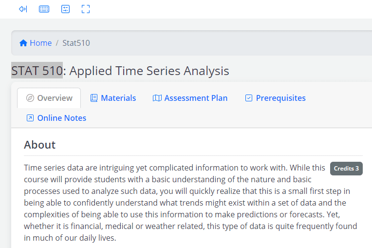
Time series data are intriguing yet complicated information to work with. While this
Credits 3 course will provide students with a basic understanding of the nature and basic processes used to analyze such data, you will quickly realize that this is a small first step in being able to confidently understand what trends might exist within a set of data and the complexities of being able to use this information to make predictions or forecasts. Yet, whether it is financial, medical or weather related, this type of data is quite frequently found in much of our daily lives.
PREREQUISITES
Topics typically covered in this graduate level course include:
- Understanding the characteristics of time series data
- Understanding moving average models and partial autocorrelation as foundations for analysis of time series data
- Exploratory Data Analysis – Trends in time series data
- Using smoothing and removing trends when working with time series data
- Understanding how periodograms are used with time series data
- Implementing ARMA and ARIMA time series models
- Identifying and interpreting various patterns for intervention effects
- Examining the analysis of repeated measures design
- Using ARCH and AR models in multivariate time series contexts
- Using spectral density estimation and spectral analysis
- Using fractional differencing and threshold models with time series data
STAT510 Time-Series Analysis HELP(EXAM HELP, ONLINE TUTOR)
Problem-1: Consider MA $(q): y_t=\sum_{j=0}^q \beta_j \epsilon_{t-j}$, where $\beta_0=1$ and $\epsilon_t$ is a white noise with variance $\sigma^2$.
(a) Compute $\mu \equiv E\left[y_t\right]$.
(b) Compute $\gamma_0 \equiv E\left[\left(y_t-\mu\right)^2\right]$.
(c) Compute $\gamma_j \equiv E\left[\left(y_t-\mu\right)\left(y_{t-j}-\mu\right)\right]$ for $j \geq 1$. (Remark: It is important to observe that $\gamma_j=0$ for $j \geq q+1$.)
(d) Conclude that $\left{y_t\right}$ is covariance stationary whatever $\beta_1, \ldots, \beta_q$ are.
(a) The mean of the MA(q) process is $\mu = E[y_t] = E\left[\sum_{j=0}^q \beta_j \epsilon_{t-j}\right]$. Since $\epsilon_t$ is a white noise process, $E[\epsilon_t] = 0$ for all $t$, so we have:
$$\mu = E\left[\sum_{j=0}^q \beta_j \epsilon_{t-j}\right] = \sum_{j=0}^q \beta_j E[\epsilon_{t-j}] = 0$$
Therefore, the mean of the MA(q) process is always zero.
(b) To compute $\gamma_0$, we start by expanding the square in the definition of $\gamma_0$:
$$\gamma_0 = E[(y_t-\mu)^2] = E\left[\left(\sum_{j=0}^q \beta_j \epsilon_{t-j}\right)^2\right] = E\left[\sum_{j=0}^q \beta_j^2 \epsilon_{t-j}^2 + 2\sum_{j=0}^{q-1} \sum_{k=j+1}^q \beta_j \beta_k \epsilon_{t-j} \epsilon_{t-k}\right]$$
Since $\epsilon_t$ is a white noise process with variance $\sigma^2$, we have $E[\epsilon_t^2] = \sigma^2$ for all $t$, and $E[\epsilon_t \epsilon_s] = 0$ for $t \neq s$. Therefore:
$$\gamma_0 = \sum_{j=0}^q \beta_j^2 \sigma^2$$
(c) For $j \geq 1$, we have:
\begin{align*} \gamma_j &= E[(y_t-\mu)(y_{t-j}-\mu)] \ &= E\left[\left(\sum_{i=0}^q \beta_i \epsilon_{t-i}\right)\left(\sum_{k=0}^q \beta_k \epsilon_{t-j-k}\right)\right] \ &= E\left[\sum_{i=0}^q \sum_{k=0}^q \beta_i \beta_k \epsilon_{t-i} \epsilon_{t-j-k}\right] \ &= \sum_{i=0}^q \sum_{k=0}^q \beta_i \beta_k E[\epsilon_{t-i} \epsilon_{t-j-k}] \end{align*}
If $j > q$, then $t-j-k < t-q \leq t$, and $\epsilon_t$ is independent of $\epsilon_{t-j-k}$, so $E[\epsilon_{t-i} \epsilon_{t-j-k}] = 0$ for all $i$ and $k$, and we have $\gamma_j = 0$. If $j \leq q$, then we have:
$$\gamma_j = \sum_{i=0}^{q-j} \beta_i \beta_{i+j} \sigma^2$$
(d) To show that ${y_t}$ is covariance stationary, we need to show that $\mu$ and $\gamma_j$ are finite and do not depend on $t$. We have already shown that $\mu = 0$ and that $\gamma_j$ is finite and depends only on $\beta_0, \ldots, \beta_q$ for $j \leq q$. To see that $\gamma_j$ does not depend on $t$, note
Problem-2: In class we covered $\mathrm{AR}(1)$ and $\mathrm{MA}(1)$ processes. Here we consider a more general process called ARMA $(1,1)$ :
$$
y_t=\phi y_{t-1}+\epsilon_t+\beta \epsilon_{t-1}
$$
where $\epsilon_t$ is a white noise with variance $\sigma^2$. Assume $|\phi|<1$ so that $\left{y_t\right}$ is covariance stationary. (Remark: $\beta$ does not play any role for covariance stationarity.) Let us compute autocorrelation functions $\rho_j$ using the Yule-Walker equations.
(a) Show that $\gamma_0=\phi \gamma_1+\sigma^2+\beta(\phi+\beta) \sigma^2$.
(b) Show that $\gamma_1=\phi \gamma_0+\beta \sigma^2$.
(c) Combining (a) and (b), solve for $\gamma_0$ and $\gamma_1$.
(d) Show that
$$
\rho_1=\frac{(\phi+\beta)(1+\phi \beta)}{1+\phi \beta+\beta(\phi+\beta)}
$$
(e) Show that $\gamma_j=\phi \gamma_{j-1}$ for $j \geq 2$.
(a) We have \begin{align*} \gamma_0 &= \operatorname{Var}(y_t) \ &= \operatorname{Var}(\phi y_{t-1} + \epsilon_t + \beta \epsilon_{t-1}) \ &= \phi^2 \operatorname{Var}(y_{t-1}) + \operatorname{Var}(\epsilon_t) + \beta^2 \operatorname{Var}(\epsilon_{t-1}) + 2\phi \operatorname{Cov}(y_{t-1}, \epsilon_t) + 2\beta \operatorname{Cov}(\epsilon_{t-1}, \epsilon_t) \ &= \phi^2 \gamma_0 + \sigma^2 + \beta^2 \sigma^2 + 2\phi \gamma_1 \end{align*} using the fact that $\operatorname{Var}(\epsilon_t) = \sigma^2$ and $\operatorname{Var}(\epsilon_{t-1}) = \sigma^2$, and that $\operatorname{Cov}(y_{t-1}, \epsilon_t) = 0$ and $\operatorname{Cov}(\epsilon_{t-1}, \epsilon_t) = 0$ since $\epsilon_t$ is a white noise process.
(b) We have \begin{align*} \gamma_1 &= \operatorname{Cov}(y_t, y_{t-1}) \ &= \operatorname{Cov}(\phi y_{t-1} + \epsilon_t + \beta \epsilon_{t-1}, y_{t-1}) \ &= \phi \operatorname{Cov}(y_{t-1}, y_{t-1}) + \beta \operatorname{Cov}(\epsilon_{t-1}, y_{t-1}) \ &= \phi \gamma_0 + \beta \sigma^2 \end{align*}
(c) Rearranging the two equations above, we have
\gamma_0 = \frac{\sigma^2 + \beta^2 \sigma^2}{1 – \phi^2} – \frac{2\beta \phi \sigma^2}{1 – \phi^2} \gamma_1γ0=1−ϕ2σ2+β2σ2−1−ϕ22βϕσ2γ1
and
\gamma_1 = \frac{\phi \gamma_0 + \beta \sigma^2}{1 – \phi^2}γ1=1−ϕ2ϕγ0+βσ2
Multiplying the first equation by $\phi$ and subtracting the second equation, we get
\gamma_0 = \frac{\sigma^2 + \beta^2 \sigma^2 – 2\beta \phi \sigma^2 \left(\phi + \frac{\beta}{1 – \phi^2}\right)}{1 – \phi^2 + 2\phi^2 \left(\phi + \frac{\beta}{1 – \phi^2}\right)}γ0=1−ϕ2+2ϕ2(ϕ+1−ϕ2β)σ2+β2σ2−2βϕσ2(ϕ+1−ϕ2β)
and
\gamma_1 = \frac{\phi \beta \sigma^2 + \phi \beta \phi \gamma_0}{1 – \phi^2 + 2\phi^2 \left(\phi + \frac{\beta}{1 – \phi^2}\right)}γ1=1−ϕ2+2ϕ2(ϕ+1−ϕ2β)ϕβσ2+ϕβϕγ0
which simplifies to
\gamma_0 = \frac{\sigma^2 + \beta^2 \sigma^2 + 2\beta\phi\sigma^2}{1 – \phi^2 – 2\beta\phi^2}γ0=1−ϕ2−2βϕ2σ2+β2σ2+2βϕσ2
Textbooks
• An Introduction to Stochastic Modeling, Fourth Edition by Pinsky and Karlin (freely
available through the university library here)
• Essentials of Stochastic Processes, Third Edition by Durrett (freely available through
the university library here)
To reiterate, the textbooks are freely available through the university library. Note that
you must be connected to the university Wi-Fi or VPN to access the ebooks from the library
links. Furthermore, the library links take some time to populate, so do not be alarmed if
the webpage looks bare for a few seconds.

Statistics-lab™可以为您提供psu.edu STAT510 Time-Series Analysis时间序列分析的代写代考和辅导服务! 请认准Statistics-lab™. Statistics-lab™为您的留学生涯保驾护航。