电气工程代写 - 统计代写答疑辅导

分类：电气工程代写

电气工程代写|通讯系统作业代写communication system代考|ELN234

Posted on 2022年10月22日2022年10月22日 by statistics-lab

如果你也在怎样代写通讯系统communication system这个学科遇到相关的难题，请随时右上角联系我们的24/7代写客服。

通信系统是一个描述两点之间信息交流的系统。信息的传输和接收过程被称为通信。通信的主要要素是信息的发送者、通信的渠道或媒介以及信息的接收者。

statistics-lab™ 为您的留学生涯保驾护航在代写通讯系统communication system方面已经树立了自己的口碑, 保证靠谱, 高质且原创的统计Statistics代写服务。我们的专家在代写通讯系统communication system方面经验极为丰富，各种代写通讯系统communication system相关的作业也就用不着说。

我们提供的通讯系统communication system及其相关学科的代写，服务范围广, 其中包括但不限于:

Statistical Inference 统计推断
Statistical Computing 统计计算
Advanced Probability Theory 高等楖率论
Advanced Mathematical Statistics 高等数理统计学
(Generalized) Linear Models 广义线性模型
Statistical Machine Learning 统计机器学习
Longitudinal Data Analysis 纵向数据分析
Foundations of Data Science 数据科学基础

电气工程代写|通讯系统作业代写communication system代考|ELN234

电气工程代写|通讯系统作业代写communication system代考|Over-rotation during electro-optical sampling

It is noted in Formula (7) that the modulation is bounded by $-1$ and 1 for phase differences of $-\pi / 2$ and $\pi / 2$, respectively. If the phase difference exceeds $\pi / 2$, the modulation decreases instead of increases since it has a sinusoidal behavior. This problem related to electro-optical detection is called over-rotation. Since a large phase difference is usually caused by a high electric field, EOS can only be used for detecting weak THz fields if over-rotation is to be avoided.

There are of course ways to work around the over-rotation problem and detect high THz fields. According to Formula (6), a smaller phase difference can be obtained by using a thinner detection crystal or having a lower electro-optical coefficient. In the first case, it should be known that a THz pulse incident on a crystal always generates reflections, which can also be detected. The thinner the crystal, the closer the reflection is temporally to the main pulse, and therefore, the more it is necessary to reduce the time window of the measurement in order to avoid measuring the reflection. However, a short time window also means a low frequency resolution, which is generally undesirable. In addition, a thinner crystal also means a shorter interaction length of the waves in the crystal, which results in a decrease in the Signalto-Noise Ratio (SNR). In the second case, it is actually possible to use a crystal with a lower electro-optical coefficient than $\mathrm{ZnTe}$, for example, gallium phosphide (GaP), and with which it is much more difficult to obtain over-rotation. On the other hand, the measured signal-to-noise ratio is then lower.

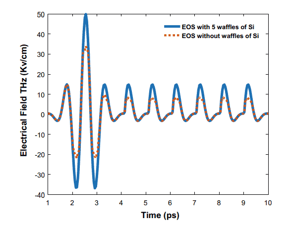
The most common solution to over-rotation is the addition of silicon waffles in the mounting just before the detection crystal (see Fig. 3). Part of the THz pulse (30\%) is reflected on each silicon waffle. The goal is to add enough silicon waffles so that the THz field reaching the crystal is both under the over-rotation limit and in the linear regime $(\sin (\Delta \varphi)=\Delta \varphi)$. However, adding several silicon waffles may cause some deformations in the detected THz field. In addition, a high THz field can induce nonlinear effects in silicon and the reflection on each waffle is then lower than $30 \%$. Also, multiple $\mathrm{THz}$ reflections on the silicon waffles are always at the tail of the main pulse in a measurement, which limits the time acquisition length and therefore the frequency resolution.

Of course, if silicon waffles are added to the assembly, this must be taken into account when calculating the THz field. By also adding the reflection losses on the detection crystal, we obtain:
$$
E_{\mathrm{THz}}=\frac{d M}{2 \pi n_0^3 L r_{41} \Gamma 0.7^N}
$$
where $\Gamma$ is the transmission coefficient through the detection crystal and $N$ is the number of waffles of Si. Each waffle transmits $70 \%$ of the THz wave.

电气工程代写|通讯系统作业代写communication system代考|THz Detection by Plasma in Air

There are two methods of plasma THz detection in air called THz-ABCD. The first is $\mathrm{THz}$ Air Breakdown Coherent Detection. The principle is very similar to $\mathrm{THz}$ generation by plasma in the air: A femtosecond laser is focused in the air, which generates a plasma whose charges are accelerated. If one sends a $\mathrm{THz}$ pulse to be detected on the plasma at the same time (or almost) as the laser pulse, there will be generation of the second harmonic of the laser beam. By detecting this second harmonic using a photomultiplier tube, the THz field can be deduced:
$$
I_{2 \omega} \propto\left|E_{2 \omega}\right|^2 \propto\left(W^{(3)} E_\omega E_\omega\right)^2 E_{\mathrm{THz}}^2
$$
where $I_{2 \omega}$ is the intensity of the second harmonic of the laser, $W^{(3)}$ is the 3rd order nonlinear coefficient of the plasma, $E_\omega$ is the laser electric field, $E_{2 \omega}$ is the electric field of the second harmonic of the laser, and $E_{\mathrm{THz}}$ is the electric field THz.

Unfortunately, since we only measure the intensity of the second harmonic, we cannot measure the electric field coherently. To achieve consistent detection, a very intense laser intensity must be used. At high pump intensity, the white light generated by the plasma contains a non-negligible second harmonic component that must be considered in the calculation [31]:
$$
I_{2 \omega} \propto\left|E_{2 \omega}\right|^2 \propto\left(W^{(3)} E_\omega E_\omega\right)^2 E_{\mathrm{THz}}^2+2\left(W^{(3)} E_\omega E_\omega\right) E_{\mathrm{THz}} E_{\mathrm{SH}}^{2 \omega}+\left(E_{\mathrm{SH}}^{2 \omega}\right)^2
$$
where $E_{\mathrm{SH}}^{2 \omega}$ is the electric field of the second harmonic from the plasma.
If the field of the second harmonic coming from the plasma is high enough, the first term of Formula (11) becomes negligible and the intensity detected by the photomultiplier tube is then proportional to the electric field $\mathrm{THz}$, making the detection method consistent. Of course, a drawback is that it is not possible to detect a $\mathrm{THz}$ field that is too large (or it is necessary to compensate with the intensity of the pump laser) since the first term of Formula (11) would then no longer be negligible. The second THz method is THz Air Bias Coherent Detection (THz-ABCD). This method requires a lower laser intensity, but an $\mathrm{AC}$ electric field must be applied close to the focal point.

通讯系统代考

电气工程代写|通讯系统作业代写communication system代考|Over-rotation during electro-optical sampling

在公式 (7) 中注意到，调制的边界为 $-1$ 和 1 的相位差 $-\pi / 2$ 和 $\pi / 2$ ，分别。如果相位差超过 $\pi / 2$ ，调制减少而不是增加，因为它具有正弦行为。这个与电光检则有关的问题称为过旋转。由于大的相位差通常是由高电场引起的，为了避免过旋转， $E O S$ 只能用于检测弱太赫兹场。
当然，有一些方法可以解决过度旋转问题并检测高 THz 场。根据公式(6)，可以通过使用更薄的检测晶体或具有更低的电光系数来获得更小的相位差。在第一种情况下，应该知道入射到晶体上的太赫兹脉冲总是会产生反射，这也是可以检测到的。晶体越薄，反射在时间上越接近主脉冲，因此越需要减小测量的时间窗口以避免测量反射。然而，短时间窗口也意味着低频率分辨率，这通常是不希望的。此外，更薄的晶体还意味着晶体中波的相互作用长度更短，这会导致信橾比 (SNR) 降低。 $\mathrm{ZnTe}$ ，例如，磷化镓 (GaP)，用它来获得过度旋转要困难得多。另一方面，测得的信噪比则较低。
最常见的过度旋转解决方案是在检测晶体之前的安装中添加硅华夫饼 (见图 3)。太赫兹脉冲的一部分 (30\%) 反映在每个硅华夫饼上。目标是添加足够的硅华夫饼，以使到达晶体的太赫兹场既低于过旋转限制又处于线性状态 $(\sin (\Delta \varphi)=\Delta \varphi)$. 然而，添加几个硅华夫饼可能会导致检测到的太赫兹场发生一些变形。此外，高太赫兹场可以在硅中引起非线性效应，每个华夫饼上的反射低于 $30 \%$. 还有，多 $\mathrm{THz}$ 在测量中，硅华夫饼上的反射始终位于主脉冲的尾部，这限制了时间采集长度，从而限制了频率分辨率。
当然，如果将硅华夫饼添加到组件中，则在计算太赫兹场时必须考虑到这一点。通过增加检测晶体上的反射损耗，我们得到:
$$
E_{\mathrm{THz}}=\frac{d M}{2 \pi n_0^3 L r_{41} \Gamma 0.7^N}
$$
在哪里 $\Gamma$ 是通过检测晶体的透射系数和 $N$ 是 Si 的华夫饼数量。每个华夫饼传输 $70 \%$ 太赫兹波。

电气工程代写|通讯系统作业代写communication system代考|THz Detection by Plasma in Air

空气中的等离子太赫兹检测方法有两种，称为太赫兹-ABCD。第一个是 $T H z$ 空气击穿相干检测。原理非常相似 $\mathrm{THz}$ 通过空气中的等离子体产生：飞秒激光聚焦在空气中，产生等离子体，其电荷被加速。如果有人发送 $\mathrm{THz}$ 在等离子体上与激光脉冲同时 (或几乎) 检测到的脉冲，将产生激光束的二次堦波。通过使用光电倍增管检测该二次谐波，可以推断出太赫兹场：
$$
I_{2 \omega} \propto\left|E_{2 \omega}\right|^2 \propto\left(W^{(3)} E_\omega E_\omega\right)^2 E_{\mathrm{THz}}^2
$$
在哪里 $I_{2 \omega}$ 是激光的二次谐波的强度， $W^{(3)}$ 是等离子体的三阶非线性系数， $E_\omega$ 是激光电场， $E_{2 \omega}$ 是激光的二次谐波的电场，并且 $E_{\mathrm{THz}}$ 是电场太赫兹。
不幸的是，由于我们只测量二次谐波的强度，我们无法连贯地测量电场。为了实现一致的检测，必须使用非常强的激光强度。在高氷浦强度下，等离子体产生的白光包含不可忽略的二次谐波分量，在计算中必须考虑 [31]:
$$
I_{2 \omega} \propto\left|E_{2 \omega}\right|^2 \propto\left(W^{(3)} E_\omega E_\omega\right)^2 E_{\mathrm{THz}}^2+2\left(W^{(3)} E_\omega E_\omega\right) E_{\mathrm{THz}} E_{\mathrm{SH}}^{2 \omega}+\left(E_{\mathrm{SH}}^{2 \omega}\right)^2
$$
在哪里 $E_{\mathrm{SH}}^{2 \omega}$ 是来自等离子体的二次谐波的电场。
如果来自等离子体的二次谐波的场足够高，则公式 (11) 的第一项可以忽略不计，光电倍增管检测到的强度与电场成正比 $\mathrm{THz}$ ，使检测方法一致。当然，缺点是无法检测到 $\mathrm{THz}$ 由于公式 (11) 的第一项将不再可忽略，因此太大的场 (或必须用百浦激光器的强度进行补偿) 。第二种太赫兹方法是太赫兹空气偏置相干检测 (THz-ABCD) 。这种方法需要较低的激光强度，但 $\mathrm{AC}$ 电场必须靠近焦点施加。

电气工程代写|通讯系统作业代写communication system代考请认准statistics-lab™

统计代写请认准statistics-lab™. statistics-lab™为您的留学生涯保驾护航。统计代写|python代写代考

随机过程代考

在概率论概念中，随机过程是随机变量的集合。若一随机系统的样本点是随机函数，则称此函数为样本函数，这一随机系统全部样本函数的集合是一个随机过程。实际应用中，样本函数的一般定义在时间域或者空间域。 随机过程的实例如股票和汇率的波动、语音信号、视频信号、体温的变化，随机运动如布朗运动、随机徘徊等等。

贝叶斯方法代考

贝叶斯统计概念及数据分析表示使用概率陈述回答有关未知参数的研究问题以及统计范式。后验分布包括关于参数的先验分布，和基于观测数据提供关于参数的信息似然模型。根据选择的先验分布和似然模型，后验分布可以解析或近似，例如，马尔科夫链蒙特卡罗 (MCMC) 方法之一。贝叶斯统计概念及数据分析使用后验分布来形成模型参数的各种摘要，包括点估计，如后验平均值、中位数、百分位数和称为可信区间的区间估计。此外，所有关于模型参数的统计检验都可以表示为基于估计后验分布的概率报表。

广义线性模型代考

广义线性模型（GLM）归属统计学领域，是一种应用灵活的线性回归模型。该模型允许因变量的偏差分布有除了正态分布之外的其它分布。

statistics-lab作为专业的留学生服务机构，多年来已为美国、英国、加拿大、澳洲等留学热门地的学生提供专业的学术服务，包括但不限于Essay代写，Assignment代写，Dissertation代写，Report代写，小组作业代写，Proposal代写，Paper代写，Presentation代写，计算机作业代写，论文修改和润色，网课代做，exam代考等等。写作范围涵盖高中，本科，研究生等海外留学全阶段，辐射金融，经济学，会计学，审计学，管理学等全球99%专业科目。写作团队既有专业英语母语作者，也有海外名校硕博留学生，每位写作老师都拥有过硬的语言能力，专业的学科背景和学术写作经验。我们承诺100%原创，100%专业，100%准时，100%满意。

机器学习代写

随着AI的大潮到来，Machine Learning逐渐成为一个新的学习热点。同时与传统CS相比，Machine Learning在其他领域也有着广泛的应用，因此这门学科成为不仅折磨CS专业同学的“小恶魔”，也是折磨生物、化学、统计等其他学科留学生的“大魔王”。学习Machine learning的一大绊脚石在于使用语言众多，跨学科范围广，所以学习起来尤其困难。但是不管你在学习Machine Learning时遇到任何难题，StudyGate专业导师团队都能为你轻松解决。

多元统计分析代考

基础数据: $N$ 个样本， $P$ 个变量数的单样本，组成的横列的数据表
变量定性: 分类和顺序；变量定量：数值
数学公式的角度分为: 因变量与自变量

时间序列分析代写

随机过程，是依赖于参数的一组随机变量的全体，参数通常是时间。随机变量是随机现象的数量表现，其时间序列是一组按照时间发生先后顺序进行排列的数据点序列。通常一组时间序列的时间间隔为一恒定值（如1秒，5分钟，12小时，7天，1年），因此时间序列可以作为离散时间数据进行分析处理。研究时间序列数据的意义在于现实中，往往需要研究某个事物其随时间发展变化的规律。这就需要通过研究该事物过去发展的历史记录，以得到其自身发展的规律。

回归分析代写

多元回归分析渐进（Multiple Regression Analysis Asymptotics）属于计量经济学领域，主要是一种数学上的统计分析方法，可以分析复杂情况下各影响因素的数学关系，在自然科学、社会和经济学等多个领域内应用广泛。

MATLAB代写

MATLAB 是一种用于技术计算的高性能语言。它将计算、可视化和编程集成在一个易于使用的环境中，其中问题和解决方案以熟悉的数学符号表示。典型用途包括：数学和计算算法开发建模、仿真和原型制作数据分析、探索和可视化科学和工程图形应用程序开发，包括图形用户界面构建MATLAB 是一个交互式系统，其基本数据元素是一个不需要维度的数组。这使您可以解决许多技术计算问题，尤其是那些具有矩阵和向量公式的问题，而只需用 C 或 Fortran 等标量非交互式语言编写程序所需的时间的一小部分。MATLAB 名称代表矩阵实验室。MATLAB 最初的编写目的是提供对由 LINPACK 和 EISPACK 项目开发的矩阵软件的轻松访问，这两个项目共同代表了矩阵计算软件的最新技术。MATLAB 经过多年的发展，得到了许多用户的投入。在大学环境中，它是数学、工程和科学入门和高级课程的标准教学工具。在工业领域，MATLAB 是高效研究、开发和分析的首选工具。MATLAB 具有一系列称为工具箱的特定于应用程序的解决方案。对于大多数 MATLAB 用户来说非常重要，工具箱允许您学习和应用专业技术。工具箱是 MATLAB 函数（M 文件）的综合集合，可扩展 MATLAB 环境以解决特定类别的问题。可用工具箱的领域包括信号处理、控制系统、神经网络、模糊逻辑、小波、仿真等。

R语言代写	问卷设计与分析代写
PYTHON代写	回归分析与线性模型代写
MATLAB代写	方差分析与试验设计代写
STATA代写	机器学习/统计学习代写
SPSS代写	计量经济学代写
EVIEWS代写	时间序列分析代写
EXCEL代写	深度学习代写
SQL代写	各种数据建模与可视化代写

电气工程代写|通讯系统作业代写communication system代考|ECE3614

Posted on 2022年10月22日2022年10月22日 by statistics-lab

如果你也在怎样代写通讯系统communication system这个学科遇到相关的难题，请随时右上角联系我们的24/7代写客服。

我们提供的通讯系统communication system及其相关学科的代写，服务范围广, 其中包括但不限于:

Statistical Inference 统计推断
Statistical Computing 统计计算
Advanced Probability Theory 高等楖率论
Advanced Mathematical Statistics 高等数理统计学
(Generalized) Linear Models 广义线性模型
Statistical Machine Learning 统计机器学习
Longitudinal Data Analysis 纵向数据分析
Foundations of Data Science 数据科学基础

电气工程代写|通讯系统作业代写communication system代考|ECE3614

电气工程代写|通讯系统作业代写communication system代考|THz Detection by Photoconductive Antennas

The principle of detection by photoconductive antennas is similar to that of generation. As for the generation, a laser pulse (visible or infrared) is sent to the semiconductor component of the antenna, between the two electrodes, in order to reduce its resistance. On the other hand, unlike the generation, no potential difference is imposed between the electrodes; here, it is the incident THz field which acts on the displacement of the photoporters. A current can then pass between the two electrodes. By measuring this current, we can determine the $\mathrm{THz}$ field using the expression that binds the two, i.e., [25]:
$$
I(t)=\int_{-\infty}^t \epsilon\left(t-t^{\prime}\right) E_{\mathrm{THz}} \mathrm{d} t^{\prime}
$$
where $I(t)$ is the current induced by the $\mathrm{THz}$ field, $\epsilon$ is the surface conductivity of the semiconductor, and $E_{\mathrm{TH} z}$ is the electric field $\mathrm{THz}$.

Photoconductive antennas are mainly used for the detection of low and medium high $\mathrm{THz}$ electric fields. Indeed, a strong $\mathrm{THz}$ electric field could induce nonlinear effects in the semiconductor and the above formula would then no longer be valid [13].

Generally, the detection of terahertz radiation using photoconductive antennas is quite similar to its emission: This time it is the incident terahertz electric field which induces a voltage between two arms of the antenna connected by a transmission line to a current amplifier. Indeed, a laser pulse excites charge carriers beyond the bandgap of the semiconductor photoswitch. The charge carriers are accelerated by the external terahertz field to be detected, such that, still in the context of the Drude model. The current measured by an ammeter is then the convolution of the sampling field $E_S^{(d)}$ and the flow of charge carriers in the detector antenna:
$$
I^{(d)}(t)=E_S^{(d)} *\left(e n^{(d)}(t) V(t)\right)
$$

电气工程代写|通讯系统作业代写communication system代考|THz Detection by Electro-Optical Sampling

Electro-optical sampling (EOS) is a technique based on the Pockels effect, which is the inverse of optical rectification. The Pockels effect is the induction of birefringence in a nonlinear crystal by a DC wave. In the case of THz detection by electro-optical sampling, it will be approximated that the $\mathrm{THz}$ wave is a DC wave since its frequency is much smaller than the visible or near infrared wave used as a probe. The THz wave is therefore sent on a non-centrosymmetric crystal, which induces a change in the polarization ellipsoid in the crystal, and therefore in the ellipsoid of the refractive indices of the crystal. For example, for a ZnTe crystal (or any other crystal with a blende-like structure), the ellipsoid of indices becomes [28]:
$$
\frac{\alpha^2+\beta^2+\gamma^2}{n_0^2}+2 r_{41} E_\alpha \beta \gamma+2 r_{41} E_\beta \alpha \gamma+2 r_{41} E_\gamma \alpha \beta=1
$$
where $\alpha, \beta, \gamma$ are the spatial coordinates corresponding to the axes of the crystal, $n_0$ is the refractive index of the crystal without exposure $\mathrm{THz}, r_{41}$ is the electro-optical coefficient of the crystal and $E_\alpha, E_\beta, E_\gamma$, are the electric fields $\mathrm{THz}$ applied along the axes $\alpha, \beta, \gamma$.

The THz wave thus induces a birefringence in the nonlinear crystal. This birefringence is probed by a second beam sent on the crystal. This beam, visible, or near infrared undergoes a change in polarization during its passage in the birefringent crystal since the optical component parallel to the slow axis of the crystal undergoes a phase delay with respect to the optical component parallel to the fast axis of the crystal [28]:
$$
\Delta \varphi=\frac{2 \pi L}{d} \Delta n
$$
where $\Delta \varphi$ is the induced phase difference, $L$ is the thickness of the crystal $d$ is the central wavelength of the probe pulse and $\Delta n$ is the difference between the refractive indices of the slow and fast axes of the crystal. For a beam orthogonal to an oriented ZnTe crystal (110) with an electric field oriented along the axis $(-110)$ of the crystal, i.e., the optimal position [29]:
$$
\Delta \varphi=\frac{2 \pi n_0^3 L r_{41} E_{\mathrm{THz}}}{d}
$$

通讯系统代考

电气工程代写|通讯系统作业代写communication system代考|THz Detection by Photoconductive Antennas

光电导天线的检测原理与发电原理类似。至于产生，激光脉冲 (可见光或红外线) 被发送到天线的半导体组件，在两个电极之间，以降低其电阻。另一方面，与生成不同，电极之间没有施加电位差。在这里，入射太赫兹场作用于光电载体的位移。然后电流可以在两个电极之间通过。通过测量这个电流，我们可以确定 $\mathrm{THz}$ 字段使用绑定两者的表达式，即[25]:
$$
I(t)=\int_{-\infty}^t \epsilon\left(t-t^{\prime}\right) E_{\mathrm{THz}} \mathrm{d} t^{\prime}
$$
在哪里 $I(t)$ 是由感应电流 $\mathrm{THz}$ 场地， $\epsilon$ 是半导体的表面电导率，并且 $E_{\mathrm{TH} z}$ 是电场 $\mathrm{THz}$.
光电导天线主要用于检测低、中高 $\mathrm{THz}$ 电场。确实，强 $\mathrm{THz}$ 电场会在半导体中引起非线性效应，因此上述公式将不再有效[13]。
通常，使用光电导天线检测太赫兹辐射与其发射非常相似：这次是入射太赫兹电场在通过传输线连接到电流放大器的天线的两个臂之间感应出电压。实际上，激光脉冲会激发超出半导体光电开关带隙的电荷载流子。电荷载流子被要检测的外部太赫兹场加速，这样，仍然在 Drude 模型的上下文中。电流表测量的电流是采样场的卷积 $E_S^{(d)}$ 以及探测器天线中电荷载流子的流动:
$$
I^{(d)}(t)=E_S^{(d)} *\left(e n^{(d)}(t) V(t)\right)
$$

电气工程代写|通讯系统作业代写communication system代考|THz Detection by Electro-Optical Sampling

电光采样 (EOS) 是一种基于普克尔斯效应的技术，它是光学整流的倒数。普克尔斯效应是直流波在非线性晶体中引起的双折射。在通过电光采样进行太赫兹探测的情况下，将近似为 $\mathrm{THz}$ 波是直流波，因为它的频率远小于用作探测的可见波或近红外波。因此，太赫兹波在非中心对称晶体上发送，这会导致晶体中偏振椭球发生变化，从而导致晶体折射率的椭球发生变化。例如，对于一个 ZnTe 晶体 (或任何其他具有类似混合结构的晶体)，指数的椭圆体变为 [28]:
$$
\frac{\alpha^2+\beta^2+\gamma^2}{n_0^2}+2 r_{41} E_\alpha \beta \gamma+2 r_{41} E_\beta \alpha \gamma+2 r_{41} E_\gamma \alpha \beta=1
$$
在哪里 $\alpha, \beta, \gamma$ 是对应于晶体轴的空间坐标， $n_0$ 是没有曝光的晶体的折射率 $\mathrm{THz}, r_{41}$ 是晶体的电光系数和 $E_\alpha, E_\beta, E_\gamma$, 是电场 $\mathrm{THz}$ 沿轴应用 $\alpha, \beta, \gamma$.
太赫兹波因此在非线性晶体中引起双折射。这种双折射由发送到晶体上的第二束光探测。由于平行于晶体慢轴的光学分量相对于平行于晶体快轴的光学分量经历相位延迟，这种可见光或近红外光束在通过双折射晶体期间会发生偏振变化[28]:
$$
\Delta \varphi=\frac{2 \pi L}{d} \Delta n
$$
在哪里 $\Delta \varphi$ 是感应相位差， $L$ 是晶体的厚度 $d$ 是探测脉冲的中心波长和 $\Delta n$ 是晶体慢轴和快轴的折射率之差。对于与定向的 ZnTe 晶体 (110) 正交的光束，电场沿轴定向 $(-110)$ 晶体的位置，即最佳位置[29]:
$$
\Delta \varphi=\frac{2 \pi n_0^3 L r_{41} E_{\mathrm{THz}}}{d}
$$

统计代写请认准statistics-lab™. statistics-lab™为您的留学生涯保驾护航。统计代写|python代写代考

随机过程代考

贝叶斯方法代考

广义线性模型代考

广义线性模型（GLM）归属统计学领域，是一种应用灵活的线性回归模型。该模型允许因变量的偏差分布有除了正态分布之外的其它分布。

机器学习代写

多元统计分析代考

基础数据: $N$ 个样本， $P$ 个变量数的单样本，组成的横列的数据表
变量定性: 分类和顺序；变量定量：数值
数学公式的角度分为: 因变量与自变量

时间序列分析代写

回归分析代写

MATLAB代写

R语言代写	问卷设计与分析代写
PYTHON代写	回归分析与线性模型代写
MATLAB代写	方差分析与试验设计代写
STATA代写	机器学习/统计学习代写
SPSS代写	计量经济学代写
EVIEWS代写	时间序列分析代写
EXCEL代写	深度学习代写
SQL代写	各种数据建模与可视化代写

电气工程代写|通讯系统作业代写communication system代考|ENG307

Posted on 2022年10月22日2022年10月22日 by statistics-lab

如果你也在怎样代写通讯系统communication system这个学科遇到相关的难题，请随时右上角联系我们的24/7代写客服。

我们提供的通讯系统communication system及其相关学科的代写，服务范围广, 其中包括但不限于:

Statistical Inference 统计推断
Statistical Computing 统计计算
Advanced Probability Theory 高等楖率论
Advanced Mathematical Statistics 高等数理统计学
(Generalized) Linear Models 广义线性模型
Statistical Machine Learning 统计机器学习
Longitudinal Data Analysis 纵向数据分析
Foundations of Data Science 数据科学基础

电气工程代写|通讯系统作业代写communication system代考|ENG307

电气工程代写|通讯系统作业代写communication system代考|Impact of THz on 6G Wireless Communication

The 5G network, with its additional new techniques, such as millimeter wave, massive MIMO, beamforming, small cells, and full duplex, will offer revolutionary new features compared to previous generations. Nevertheless, the explosive growth in the number of connected systems could overcome the capabilities of $5 \mathrm{G}$ wireless networks. Some recently developed applications, such as virtual reality systems, are required to go beyond $5 \mathrm{G}$ because they need a minimum data rate of ten $\mathrm{Gbps}$, which exceeds the capacity of 5G systems [43]. In addition, high-definition video, ultrahigh-definition (UHD) devices, and 3-D video are becoming increasingly valuable for mobile users. Uncompressed UHD video can achieve $24 \mathrm{~Gb} / \mathrm{s}$ data rate, while uncompressed 3-D video with UHD can achieve $100 \mathrm{G} / \mathrm{ps}$ [26].

Research into the use of $\mathrm{THz}$ radiation in $6 \mathrm{G}$ wireless networks has become a daily occupation for researchers and players in the telecommunications field. This technology will revolutionize not only communication systems and their applications, but also business, personal life, lifestyle, and thus society [44]. To meet the expectations of the intelligent information society of 2030. China has launched the “Broadband Communications and New Networks” project for 2030 and beyond. The European Commission’s Horizon 2020 program has sponsored multiple B5G projects, like TERRANOVA; a project that aims to develop architectures and technologies capable of delivering optical network quality of experience in 6G wireless communication networks [45]. In the USA, the FCC has already launched studies of $6 \mathrm{G}$ networks, and the THz band has already opened. For the FCC, frequencies beyond $5 \mathrm{G}$ are reserved for 6G. In Japan, the first 6G projects have already been launched in 2020 [46]. Finland organized the first global summit on 6G wireless technology and launched the 6Genesis project, the first $6 \mathrm{G}$ project. The project supports the development of several aspects of wireless communication [47]. The International

电气工程代写|通讯系统作业代写communication system代考|VCO Design for THz Band

Various electronic and/or photonic systems and technologies have been developed to achieve the first demonstrations of THz communication. Due to the limitation of the operating frequency of the transistors developed by different foundries, most of the published works in the literature propose photonic solutions. Recently, electronic techniques are being developed, and our work is part of the development of an efficient wireless communication system for the terahertz frequency band.

Due to the behavior of passive elements at high frequencies, and the limited cutoff frequency for transistors, the VCO presents one of the most difficult blocks to design in a transceiver system. In this section, we propose the study and design of a $\mathrm{VCO}$, capable to generate a signal with frequencies around $104 \mathrm{GHz}$.

For the design of a local oscillator that delivers a high-power signal with minimal phase noise, we have opted for the pHEMT (pseudomorphic High Electron Mobility Transistor) of the PH15 process from the UMS foundry. It is characterized by a transition frequency $\mathrm{fT}=110 \mathrm{GHz}$ and a gate length of $0.15 \mu \mathrm{m}$ [48]. In this regard, considering the limitation of the operating frequency of most of the transistors developed so far, we have focused in this chapter on the choice of a structure that favors the second harmonic (Fig. 3). It consists of a LO (Fig. 4) whose fundamental oscillation frequency is $52 \mathrm{GHz}$ and a bandpass filter (Fig. 7), whose passband is around $104 \mathrm{GHz}$.

通讯系统代考

电气工程代写|通讯系统作业代写communication system代考|Impact of THz on 6G Wireless Communication

5G 网络及其附加新技术，如毫米波、大规模 MIMO、波束成形、小型蜂窝和全双工，将提供与前几代相比具有革命性的新功能。然而，连接系统数量的爆炸式增长可能会克服5G无线网络。一些最近开发的应用程序，例如虚拟现实系统，需要超越5G因为他们需要 10 的最低数据速率Gbps，这超过了 5G 系统的容量 [43]。此外，高清视频、超高清 (UHD) 设备和 3-D 视频对移动用户的价值越来越高。未压缩的超高清视频可以实现24 Gb/s数据速率，而 UHD 的未压缩 3-D 视频可以实现100G/ps [26].

研究使用吨H和辐射6G无线网络已成为电信领域研究人员和参与者的日常工作。这项技术不仅将彻底改变通信系统及其应用，还将改变商业、个人生活、生活方式，从而改变社会[44]。为满足2030年智能信息社会的期望。中国启动了2030年及以后的“宽带通信与新网络”工程。欧盟委员会的 Horizon 2020 计划已经赞助了多个 B5G 项目，例如 TERRANOVA；一个旨在开发能够在 6G 无线通信网络中提供光网络体验质量的架构和技术的项目 [45]。在美国，FCC 已经开始研究6G网络，太赫兹频段已经开通。对于 FCC，频率超过5G为 6G 预留。在日本，首批 6G 项目已于 2020 年启动 [46]。芬兰组织首届全球6G无线技术峰会并启动6Genesis项目6G项目。该项目支持无线通信的几个方面的发展[47]。国际

电气工程代写|通讯系统作业代写communication system代考|VCO Design for THz Band

已经开发了各种电子和/或光子系统和技术来实现太赫兹通信的首次演示。由于不同代工厂开发的晶体管工作频率的限制，文献中发表的大部分作品都提出了光子解决方案。最近，电子技术正在开发中，我们的工作是开发用于太赫兹频段的高效无线通信系统的一部分。

由于无源元件在高频下的行为以及晶体管的有限截止频率，VCO 是收发器系统中最难设计的模块之一。在本节中，我们建议研究和设计一个在C○, 能够产生频率约为104GH和.

为了设计能够提供具有最小相位噪声的高功率信号的本地振荡器，我们选择了来自 UMS 代工厂的 PH15 工艺的 pHEMT（伪高电子迁移率晶体管）。它的特点是过渡频率F吨=110GH和和栅极长度0.15米米[48]。在这方面，考虑到迄今为止开发的大多数晶体管的工作频率的限制，我们在本章中将重点放在选择有利于二次谐波的结构上（图 3）。它由一个 LO（图 4）组成，其基本振荡频率为52GH和和一个带通滤波器（图 7），其通带约为104GH和.

统计代写请认准statistics-lab™. statistics-lab™为您的留学生涯保驾护航。统计代写|python代写代考

随机过程代考

贝叶斯方法代考

广义线性模型代考

广义线性模型（GLM）归属统计学领域，是一种应用灵活的线性回归模型。该模型允许因变量的偏差分布有除了正态分布之外的其它分布。

机器学习代写

多元统计分析代考

基础数据: $N$ 个样本， $P$ 个变量数的单样本，组成的横列的数据表
变量定性: 分类和顺序；变量定量：数值
数学公式的角度分为: 因变量与自变量

时间序列分析代写

回归分析代写

MATLAB代写

R语言代写	问卷设计与分析代写
PYTHON代写	回归分析与线性模型代写
MATLAB代写	方差分析与试验设计代写
STATA代写	机器学习/统计学习代写
SPSS代写	计量经济学代写
EVIEWS代写	时间序列分析代写
EXCEL代写	深度学习代写
SQL代写	各种数据建模与可视化代写

电气工程代写|数字系统设计作业代写Digital System Design代考|COE328

Posted on 2022年10月22日2022年10月22日 by statistics-lab

如果你也在怎样代写数字系统设计Digital System Design这个学科遇到相关的难题，请随时右上角联系我们的24/7代写客服。

数字系统设计课程侧重于从头开始设计数字系统。该课程的重点是设计组合和顺序构件，使用这些构件来设计更大的数字系统。

statistics-lab™ 为您的留学生涯保驾护航在代写数字系统设计Digital System Design方面已经树立了自己的口碑, 保证靠谱, 高质且原创的统计Statistics代写服务。我们的专家在代写数字系统设计Digital System Design方面经验极为丰富，各种代写数字系统设计Digital System Design相关的作业也就用不着说。

我们提供的数字系统设计Digital System Design及其相关学科的代写，服务范围广, 其中包括但不限于:

Statistical Inference 统计推断
Statistical Computing 统计计算
Advanced Probability Theory 高等楖率论
Advanced Mathematical Statistics 高等数理统计学
(Generalized) Linear Models 广义线性模型
Statistical Machine Learning 统计机器学习
Longitudinal Data Analysis 纵向数据分析
Foundations of Data Science 数据科学基础

电气工程代写|数字系统设计作业代写Digital System Design代考|COE328

电气工程代写|数字系统设计作业代写Digital System Design代考|Transmitter Antenna Losses

Several losses are associated with the antenna. Some of the possible losses, which may or may not be present in each antenna, are as follows:

$L_{t r}$, radome losses on the transmitter antenna. The radome is the covering over the antenna that protects the antenna from the outside elements. Most antennas do not require a radome.
$L_{t p o l}$, polarization mismatch losses. Many antennas are polarized (i.e., horizontal, vertical, or circular). This defines the spatial position or orientation of the electric and magnetic fields. A mismatch loss is due to the polarization of the transmitter antenna being spatially off with respect to the receiver antenna. The amount of loss is equal to the angle difference between them. For example, if both the receiver and transmitter antennas are vertically polarized, they would be at $90^{\circ}$ from the earth. If one is positioned at $80^{\circ}$ and the other is positioned at $100^{\circ}$, the difference is $20^{\circ}$. Therefore, the loss due to polarization would be
$$
20 \log (\cos \theta)=20 \log (\cos 20)=0.54 \mathrm{~dB}
$$
$L_{t f o c}$, focusing loss or refractive loss. This is caused by imperfections in the shape of the antenna so that the energy is focused toward the feed. This is often a factor when the antenna receives signals at low elevation angles.
$L_{\text {tpoint }}$, mispointed loss. This is caused by transmitting and receiving directional antennas that are not exactly lined up and pointed toward each other. Thus, the gains of the antennas do not add up without a loss of signal power.
$L_{\text {tcon, }}$ conscan crossover loss. This loss is present only if the antenna is scanned in a circular search pattern, such as a conscan (conical scan) radar searching for a target. Conscan means that the antenna system is either electrically or mechanically scanned in a conical fashion or in a cone-shaped pattern. This is used in radar and other systems that desire a broader band of spatial coverage but must maintain a narrow beam width. This is also used for generating the pointing error for a tracking antenna.

电气工程代写|数字系统设计作业代写Digital System Design代考|Transmitted Effective Isotropic Radiated Power

An isotropic radiator is a theoretical radiator that assumes a point source radiating in all directions. Effective isotropic radiated power (EIRP) is the amount of power from a single point radiator that is required to equal the amount of power that is transmitted by the power amplifier, losses, and directivity of the antenna (antenna gain) in the direction of the receiver.

The EIRP provides a way to compare different transmitters. To analyze the output of an antenna, EIRP is used (Figure 1-2):
$$
\operatorname{EIRP}=P_t-L_{t t}+G_t-L_{t o}
$$
where
$P_t=$ transmitter power in $\mathrm{dBm}$
$L_{t t}=$ total negative losses in $\mathrm{dB}$; coaxial or waveguide line losses, switchers, circulators, antenna connections
$G_t=$ transmitter antenna gain in $\mathrm{dB}$ referenced to a isotropic antenna
$L_{t a}=$ total transmitter antenna losses in $\mathrm{dB}$
Effective radiated power (ERP) is another term used to describe the output power of an antenna. However, instead of comparing the effective power to an isotropic radiator, the power output of the antenna is compared to a dipole antenna. The relationship between EIRP and ERP is
$$
\mathrm{EIRP}=\mathrm{ERP}+G_{\text {dipole }},
$$
where $G_{\text {dipole }}$ is the gain of a dipole antenna, which is equal to approximately $2.14 \mathrm{~dB}$ (Figure 1-2). For example,
$$
\begin{aligned}
\mathrm{EIRP} &=10 \mathrm{dBm} \
\mathrm{ERP} &=\mathrm{EIRP}-G_{\text {dipole }}=10 \mathrm{dBm}-2.14 \mathrm{~dB}=7.86 \mathrm{dBm}
\end{aligned}
$$

数字系统设计代考

电气工程代写|数字系统设计作业代写Digital System Design代考|Transmitter Antenna Losses

一些损耗与天线有关。每个天线中可能存在也可能不存在的一些可能的损耗如下:

$L_{t r}$ ，发射机天线上的天线罩损耗。天线罩是天线上的覆盖物，可保护天线免受外部元件的影响。大多数天线不需要天线罩。
$L_{t p o l}$ ，极化失配损失。许多天线是极化的（即水平、垂直或圆形）。这定义了电场和磁场的空间位置或方向。失配损耗是由于发射器天线的极化相对于接收器天线在空间上偏离。损失量等于它们之间的角度差。例如，如果接收器和发射器天线都是垂直极化的，它们将在 $90^{\circ}$ 来自地球。如果一个位于 $80^{\circ}$ 另一个位于 $100^{\circ}$ ，区别是 $20^{\circ}$. 因此，极化引起的损耗为
$$
20 \log (\cos \theta)=20 \log (\cos 20)=0.54 \mathrm{~dB}
$$
$L_{t f o c}$ ，聚焦损失或屈光损失。这是由天线形状的缺陷引起的，因此能量集中在馈源上。当天线以低仰角接收信号时，这通常是一个因素。
$L_{\text {tpoint }}$ ，误点损失。这是由于发射和接收定向天线末完全对齐并相互指向造成的。因此，天线的增益不会在没有信号功率损失的情况下相加。
$L_{\text {tcon, }}$ conscan 交叉损失。仅当以圆形搜索模式扫描天线时才会出现这种损失，例如搜索目标的 conscan (锥形扫描) 雷达。Conscan 意味着天线系统以雉形方式或以雉形图案进行电气或机械扫描。这用于雷达和其他需要更宽的空间覆盖范围但必须保持窄波束宽度的系统。这也用于生成跟踪天线的指向误差。

电气工程代写|数字系统设计作业代写Digital System Design代考|Transmitted Effective Isotropic Radiated Power

各向同性辐射体是一种理论辐射体，它假设点源向所有方向辐射。有效全向辐射功率 (EIRP) 是来自单点辐射器的功率量，它需要等于功率放大器发射的功率量、损耗和天线方向上的天线方向性 (天线增益)。接收者。
EIRP 提供了一种比较不同发射机的方法。为了分析天线的输出，使用了 EIRP (图 1-2)：
$$
\mathrm{EIRP}=P_t-L_{t t}+G_t-L_{t o}
$$
在哪里
$P_t=$ 发射机功率 $\mathrm{dBm}$
$L_{t t}=$ 总负损失 $\mathrm{dB} ;$ 同轴或波导线路损耗、开关、环行器、天线连接
$G_t=$ 发射机天线增益 $\mathrm{dB}$ 参考各向同性天线
$L_{t a}=$ 总发射机天线损耗 $\mathrm{dB}$
有效辐射功率 (ERP) 是用于描述天线输出功率的另一个术语。但是，不是将有效功率与各向同性辐射器进行比较，而是将天线的功率输出与偶极天线进行比较。EIRP和ERP之间的关系是
$$
\mathrm{EIRP}=\mathrm{ERP}+G_{\text {dipole }},
$$
在哪里 $G_{\text {dipole }}$ 是偶极天线的增益，大约等于 $2.14 \mathrm{~dB}$ (图 1-2) 。例如，
$$
\mathrm{EIRP}=10 \mathrm{dBm} \mathrm{ERP} \quad=\mathrm{EIRP}-G_{\text {dipole }}=10 \mathrm{dBm}-2.14 \mathrm{~dB}=7.86 \mathrm{dBm}
$$

电气工程代写|数字系统设计作业代写Digital System Design代考请认准statistics-lab™

统计代写请认准statistics-lab™. statistics-lab™为您的留学生涯保驾护航。统计代写|python代写代考

随机过程代考

贝叶斯方法代考

广义线性模型代考

广义线性模型（GLM）归属统计学领域，是一种应用灵活的线性回归模型。该模型允许因变量的偏差分布有除了正态分布之外的其它分布。

机器学习代写

多元统计分析代考

基础数据: $N$ 个样本， $P$ 个变量数的单样本，组成的横列的数据表
变量定性: 分类和顺序；变量定量：数值
数学公式的角度分为: 因变量与自变量

时间序列分析代写

回归分析代写

MATLAB代写

R语言代写	问卷设计与分析代写
PYTHON代写	回归分析与线性模型代写
MATLAB代写	方差分析与试验设计代写
STATA代写	机器学习/统计学习代写
SPSS代写	计量经济学代写
EVIEWS代写	时间序列分析代写
EXCEL代写	深度学习代写
SQL代写	各种数据建模与可视化代写

电气工程代写|数字系统设计作业代写Digital System Design代考|EE301

Posted on 2022年10月22日2022年10月22日 by statistics-lab

如果你也在怎样代写数字系统设计Digital System Design这个学科遇到相关的难题，请随时右上角联系我们的24/7代写客服。

数字系统设计课程侧重于从头开始设计数字系统。该课程的重点是设计组合和顺序构件，使用这些构件来设计更大的数字系统。

我们提供的数字系统设计Digital System Design及其相关学科的代写，服务范围广, 其中包括但不限于:

Statistical Inference 统计推断
Statistical Computing 统计计算
Advanced Probability Theory 高等楖率论
Advanced Mathematical Statistics 高等数理统计学
(Generalized) Linear Models 广义线性模型
Statistical Machine Learning 统计机器学习
Longitudinal Data Analysis 纵向数据分析
Foundations of Data Science 数据科学基础

电气工程代写|数字系统设计作业代写Digital System Design代考|EE301

电气工程代写|数字系统设计作业代写Digital System Design代考|Transmitter Component Losses

Most transceiver systems contain RF components such as a circulator or a transmit/receive (T/R) switch that enable the transceiver to use the same antenna for both transmitting and receiving. Also, if the antenna arrays use multiple antennas, some of their components will interconnect the individual antenna elements. Since these elements have a loss associated with them, they need to be taken into account in the overall output power of the transmitter. These losses directly reduce the signal level or the power output of the transmitter. The component losses are labeled and are included in the analysis:
$L_{\text {tcomp }}=$ switchers, circulators, antenna connections
Whichever method is used, the losses directly affect the power output on a one-for-one basis. A $1 \mathrm{~dB}$ loss equals a $1 \mathrm{~dB}$ loss in transmitted power. Therefore, the losses after the final output power amplifier (PA) of the transmitter and the first amplifier (or low-noise amplifier [LNA]) of the receiver should be kept to a minimum. Each $\mathrm{dB}$ of loss in this path will either reduce the minimum detectable signal (MDS) by a dB or the transmitter gain will have to transmit a $\mathrm{dB}$ more power.

Since most transmitters are located at a distance from the antenna, the cable or waveguide connecting the transmitter to the antenna contains losses that need to be incorporated in the total power output:
$L_{t l l}=$ coaxial or waveguide line losses (in $\left.\mathrm{dB}\right)$
These transmitter line losses are included in the total power output analysis; a $1 \mathrm{~dB}$ loss equals a $1 \mathrm{~dB}$ loss in power output. Using larger diameter cables or higher quality cables can reduce the loss, which is a trade-off with cost. For example, heliax cables are used for very low-loss applications. However, they are generally more expensive and larger in diameter than standard cables. The total losses between the power amplifier and the antenna are therefore equal to
$$
L_{t t}=L_{t l l}+L_{\text {tcomp }}
$$
Another way to reduce the loss between the transmitter and the antenna is to locate the transmitter power amplifier as close to the antenna as possible. This will reduce the length of the cable, which reduces the overall loss in the transmitter.

电气工程代写|数字系统设计作业代写Digital System Design代考|Transmitter Antenna Gain

Most antennas experience gain because they tend to focus energy in specified directions compared with an ideal isotropic antenna, which radiates in all directions. Antennas do not amplify the signal power but focus the existing signal in a given direction. This is similar to a magnifying glass, which can be used to focus the sun rays in a specific direction, increasing the signal level at a single point (Figure 1-4).

A simple vertical dipole antenna experiences approximately $2.14 \mathrm{dBi}$ of gain compared with an isotropic radiator because it transmits most of the signal around the antenna, with very little of the signal transmitted directly up to the sky and directly down to the ground (Figure 1-5).
A parabolic dish radiator is commonly used at high frequencies to achieve gain by focusing the signal in the direction the antenna is pointing (Figure 1-6). The gain for a parabolic antenna is
$$
G_t=10 \log \left[n(\pi D / \lambda)^2\right]
$$
where
$$
\begin{aligned}
G_t &=\text { gain of the antenna (in dBi) } \
n &=\text { efficiency factor }<1 \
D &=\text { diameter of the parabolic dish } \
\lambda &=\text { wavelength }
\end{aligned}
$$

The efficiency factor is the actual gain of the antenna compared with the theoretical gain. This can happen when a parabolic antenna is not quite parabolic, when the surface of the antenna combined with the feed is not uniform, and when other anomalies occur in the actual implementation of the antenna system. Typically this ranges from $0.5$ to $0.8$, depending on the design and the frequency of operation.

Notice that the antenna gain increases both with increasing diameter and higher frequency (shorter wavelength). The gain of the antenna is a direct gain where a $1 \mathrm{~dB}$ gain equals a $1 \mathrm{~dB}$ improvement in the transmitter power output. Therefore, a larger gain will increase the range of the link. In addition, the more gain the antenna can produce, the less power the power amplifier has to deliver for the same range. This is another trade-off that needs to be considered to ensure the best design and the lowest cost for a given application.

数字系统设计代考

电气工程代写|数字系统设计作业代写Digital System Design代考|Transmitter Component Losses

大多数收发器系统都包含射频组件，例如循环器或发射/接收 (T/R) 开关，使收发器能够使用相同的天线进行发射和接收。此外，如果天线阵列使用多个天线，它们的一些组件将互连各个天线元件。由于这些元件具有与之相关的损耗，因此需要在发射器的总输出功率中考虑它们。这些损耗直接降低了发射机的信号电平或功率输出。组件损耗已标记并包含在分析中:
$L_{\text {tcomp }}=$ 切换器、循环器、天线连接
无论使用哪种方法，损耗都会一对一地直接影响功率输出。一个 $1 \mathrm{~dB}$ 损失等于 $1 \mathrm{~dB}$ 传输功率的损失。因此，发射器的最终输出功率放大器 (PA) 和接收器的第一个放大器 (或低䆆声放大器 $[L N A])$ 后的损耗应保持在最低水平。每个dB这条路径中的损耗要么将最小可检测信号 (MDS) 降低一个 $\mathrm{dB}$ ，要么发射器增益将不得不发射一个 $\mathrm{dB}$ 更多的权力。
由于大多数发射器与天线相距一定距离，因此将发射器连接到天线的电赀或波导包含需要纳入总功率输出的损耗: $L_{t l l}=$ 同轴或波导线损耗 (在 $\left.\mathrm{dB}\right)$
这些发射机线路损耗包含在总功率输出分析中; 一个 $1 \mathrm{~dB}$ 损失等于 $1 \mathrm{~dB}$ 功率输出的损失。使用更大直径的电笕或更高质量的电缆可以减少损耗，这是与成本的权衡。例如，螺旋电缆用于非常低损耗的应用。但是，它们通常比标准电跕更昂贵且直径更大。因此，功率放大器和天线之间的总损耗等于
$$
L_{t t}=L_{t l l}+L_{\text {tcomp }}
$$
另一种减少发射机和天线之间损耗的方法是将发射机功率放大器放置在尽可能靠近天线的位置。这将减少电趿的长度，从而降低发射机的整体损耗。

电气工程代写|数字系统设计作业代写Digital System Design代考|Transmitter Antenna Gain

大多数天线都能获得增益，因为与理想的各向同性天线相比，它们倾向于将能量集中在特定的方向上，而理想的各向同性天线佘向所有方向辐射。天线不会放大信号功率，而是将现有信号集中在给定方向上。这类似于放大镜，可用于将太阳光线聚焦到特定方向，从而增加单个点的信号电平 (图 1-4)。
一个简单的垂直偶极子天线大约经历 $2.14 \mathrm{dBi}$ 与各向同性辐射器相比，它的增益比各向同性辐射器高，因为它在天线周围传输大部分信号，只有很少的信号直接向上传输到天空并直接向下传输到地面（图 1-5)。
抛物面碟形辐射器通常用于高频，通过将信号聚焦在天线指向的方向来实现增益 (图 1-6)。抛物面天线的增益为
$$
G_t=10 \log \left[n(\pi D / \lambda)^2\right]
$$
在哪里
$G_t=$ gain of the antenna (in dBi) $n=$ efficiency factor $<1 D=$ diameter of the parabolic
效率因子是天线的实际增益与理论增益的比较。当抛物面天线不是完全抛物线时，当天线与馈源结合的表面不均匀，以及在天线系统的实际实现中出现其他异常时，就会发生这种情况。通常这范围从 $0.5$ 至 $0.8$ ，取决于设计和操作步跕率。
请注意，天线增益随着直径的增加和更高的频率（更短的波长）而增加。天线的增益是直接增益，其中 $1 \mathrm{~dB}$ 增益等于1 $\mathrm{dB}$ 发射机功率输出的改进。因此，较大的增益将增加链路的范围。此外，天线可以产生的增益越大，功率放大器在相同范围内必须提供的功率就越小。这是另一个需要考虑的权衡，以确保给定应用程序的最佳设计和最低成本。

统计代写请认准statistics-lab™. statistics-lab™为您的留学生涯保驾护航。统计代写|python代写代考

随机过程代考

贝叶斯方法代考

广义线性模型代考

广义线性模型（GLM）归属统计学领域，是一种应用灵活的线性回归模型。该模型允许因变量的偏差分布有除了正态分布之外的其它分布。

机器学习代写

多元统计分析代考

基础数据: $N$ 个样本， $P$ 个变量数的单样本，组成的横列的数据表
变量定性: 分类和顺序；变量定量：数值
数学公式的角度分为: 因变量与自变量

时间序列分析代写

回归分析代写

MATLAB代写

R语言代写	问卷设计与分析代写
PYTHON代写	回归分析与线性模型代写
MATLAB代写	方差分析与试验设计代写
STATA代写	机器学习/统计学习代写
SPSS代写	计量经济学代写
EVIEWS代写	时间序列分析代写
EXCEL代写	深度学习代写
SQL代写	各种数据建模与可视化代写

电气工程代写|数字系统设计作业代写Digital System Design代考|ECE4110

Posted on 2022年10月22日2022年10月22日 by statistics-lab

如果你也在怎样代写数字系统设计Digital System Design这个学科遇到相关的难题，请随时右上角联系我们的24/7代写客服。

数字系统设计课程侧重于从头开始设计数字系统。该课程的重点是设计组合和顺序构件，使用这些构件来设计更大的数字系统。

我们提供的数字系统设计Digital System Design及其相关学科的代写，服务范围广, 其中包括但不限于:

Statistical Inference 统计推断
Statistical Computing 统计计算
Advanced Probability Theory 高等楖率论
Advanced Mathematical Statistics 高等数理统计学
(Generalized) Linear Models 广义线性模型
Statistical Machine Learning 统计机器学习
Longitudinal Data Analysis 纵向数据分析
Foundations of Data Science 数据科学基础

电气工程代写|数字系统设计作业代写Digital System Design代考|ECE4110

电气工程代写|数字系统设计作业代写Digital System Design代考|Frequency of Operation

In a transceiver design, we first determine the radio frequency (RF) of operation. The frequency of operation depends on the following factors:

RF availability: This is the frequency band that is available for use by a particular system and is dependent on the communications authority for each country. For example, in the United States it is specified by the Federal Communications Commission (FCC), and in the United Kingdom it is specified by the British Approvals Board for Telecommunications (BABT). These two groups have ultimate control over frequency band allocation. Other organizations that help to establish standards are the International Telecommunications Union Standardization Sector (ITU-T), the European Conference of Postal and Telecommunications Administrations (CEPT), and the European Telecommunications Standards Institute (ETSI).
Cost: As the frequency increases, the components in the receiver tend to be more expensive. An exception to the rule is when there is a widely used frequency band, such as the cellular radio band, where supply and demand drive down the cost of parts and where integrated circuits are designed for specific applications. These are known as application-specific integrated circuits (ASICs).
Range and antenna size: As a general rule, decreasing the frequency will also decrease the amount of loss between the transmitter and the receiver. This loss is mainly due to free-space attenuation and is calculated using the frequency or wavelength of the transmission. This results in an increase in range for line-of-sight applications or a decrease in the output power requirement, which would also affect cost. However, another factor that affects range is the ability of the signal to reflect or bounce off the atmosphere, mainly the ionosphere and sometimes the troposphere. For specific frequencies, this can increase the range tremendously. Amateur radio operators use frequencies that can bounce off the atmosphere and travel around the world with less than 100 watts of power. Also, the size of the antenna increases as the frequency decreases. Therefore, the size of the antenna might be too big for practical considerations and could also be a factor in the cost of the design.

Customer specified: Oftentimes the frequency of operation is specified by the customer. If the application is for commercial applications, the frequency selection must follow the rules currently in place for that specific application to obtain the approval of the FCC and other agencies.
Band congestion: Ideally, the frequency band selected is an unused band or serves very little purpose, especially with no high-power users in the band. This also needs to be approved by the FCC and other agencies. Generally the less used bands are very high, which increases the cost. Many techniques available today allow more users to operate successfully in particular bands, and some of these techniques will be discussed further in the book.

电气工程代写|数字系统设计作业代写Digital System Design代考|Power from the Transmitter

The power from the transmitter $\left(P_t\right)$ is the amount of power output of the final stage of the power amplifier. For ease in the analysis of power levels, the power is specified in $\mathrm{dBm}$ or converted to $\mathrm{dBm}$ from milliwatts $(\mathrm{mW})$. The power in $\mathrm{mW}$ is converted to power in $\mathrm{dBm}$ by
$$
P_{\mathrm{dbm}}=10 \log P_{\mathrm{mW}}
$$
Therefore, $1 \mathrm{~mW}$ is equal to $0 \mathrm{dBm}$. The unit $\mathrm{dBm}$ is used extensively in the industry, and a good understanding of this term and other $\mathrm{dB}$ terms is important. The term $\mathrm{dBm}$ is actually a power level related to $1 \mathrm{~mW}$ and is not a loss or gain as is the term $\mathrm{dB}$.

A decibel $(\mathrm{dB})$ is a unit for expressing the ratio of two amounts of electric or acoustic signal power. The decibel is used to enable the engineer to calculate the resultant power level by simply adding or subtracting gains and losses instead of multiplying and dividing.
Gains and losses are expressed in $\mathrm{dB} . \mathrm{A} \mathrm{dB}$ is defined as a power ratio:
$$
\mathrm{dB}=10 \log \left(P_o / P_i\right)
$$
where
$P_i=$ the input power (in $\mathrm{mW}$ )
$P_o=$ the output power (in $\mathrm{mW}$ )

For example:
Given:
Amplifier power input $=0.15 \mathrm{~mW}=10 \log (0.15)=-8.2 \mathrm{dBm}$ Amplifier power gain $P_o / P_i=13=10 \log (13)=11.1 \mathrm{~dB}$
Calculate the power output:
Power output $=0.15 \mathrm{~mW} \times 13=1.95 \mathrm{~mW}$ using power and multiplication Power output (in $\mathrm{dBm}$ ) $=-8.2 \mathrm{dBm}+11.1 \mathrm{~dB}=2.9 \mathrm{dBm}$ using $\mathrm{dBm}$ and $\mathrm{dB}$ and addition
Note: $2.9 \mathrm{dBm}=10 \log (1.95)$
Another example of using $\mathrm{dBm}$ and $\mathrm{dB}$ is as follows:
In many applications, $\mathrm{dB}$ and $\mathrm{dBm}$ are misused, which can cause errors in the results. The unit $\mathrm{dB}$ is used for a change in power level, which is generally a gain or a loss. The unit $\mathrm{dBm}$ is used for absolute power; for example, $10 \log (1$ milliwatt $)=0 \mathrm{dBm}$. The unit $\mathrm{dBw}$ is also used for absolute power; for example, $10 \log (1 \mathrm{watt})=0 \mathrm{dBw}$. The terms $\mathrm{dBm}$ and $\mathrm{dBw}$ are never used for expressing a change in signal level. The following examples demonstrate this confusion.

数字系统设计代考

电气工程代写|数字系统设计作业代写Digital System Design代考|Frequency of Operation

在收发器设计中，我们首先确定工作的射频 (RF)。操作频率取决于以下因素：

RF 可用性：这是可供特定系统使用的频段，取决于每个国家/地区的通信机构。例如，在美国由联邦通信委员会 (FCC) 指定，在英国由英国电信认证委员会 (BABT) 指定。这两组对频带分配具有最终控制权。其他帮助制定标准的组织包括国际电信联盟标准化部门 (ITU-T)、欧洲邮政和电信管理会议 (CEPT) 和欧洲电信标准协会 (ETSI)。
成本：随着频率的增加，接收器中的组件往往更昂贵。该规则的一个例外是当存在广泛使用的频段时，例如蜂窝无线电频段，供需降低了零件成本，并且集成电路是为特定应用设计的。这些被称为专用集成电路（ASIC）。
范围和天线尺寸：作为一般规则，降低频率也会减少发射器和接收器之间的损耗量。这种损耗主要是由于自由空间衰减造成的，并且是使用传输的频率或波长计算得出的。这导致视距应用范围的增加或输出功率要求的降低，这也会影响成本。然而，影响范围的另一个因素是信号反射或反射大气层的能力，主要是电离层，有时是对流层。对于特定频率，这可以极大地增加范围。业余无线电操作员使用的频率可以从大气层反弹并以不到 100 瓦的功率环游世界。此外，天线的尺寸随着频率的降低而增加。

客户指定：通常操作频率由客户指定。如果申请是用于商业应用，则频率选择必须遵循该特定应用的现行规则，以获得 FCC 和其他机构的批准。
频段拥塞：理想情况下，所选频段是未使用的频段或用途很少，尤其是频段内没有高功率用户。这也需要得到 FCC 和其他机构的批准。通常较少使用的频段非常高，这增加了成本。当今可用的许多技术允许更多用户在特定频段成功操作，其中一些技术将在本书中进一步讨论。

电气工程代写|数字系统设计作业代写Digital System Design代考|Power from the Transmitter

来自发射器的功率 $\left(P_t\right)$ 是功率放大器末级的功率输出量。为了便于分析功率水平，功率在 $\mathrm{dBm}$ 或转换为 $\mathrm{dBm}$ 从毫瓦 $(\mathrm{mW})$. 中的力量 $\mathrm{mW}$ 被转换成电源 $\mathrm{dBm}$ 经过
$$
P_{\mathrm{dbm}}=10 \log P_{\mathrm{mW}}
$$
所以， $1 \mathrm{~mW}$ 等于 $0 \mathrm{dBm}$. 那个单位 $\mathrm{dBm}$ 在行业中被广泛使用，并且对该术语和其他术语有很好的理解 $\mathrm{dB}$ 条款很重要。期限 $\mathrm{dBm}$ 实际上是一个与功率级别有关的 $1 \mathrm{~mW}$ 并且不是术语的损失或收益 $\mathrm{dB}$.
分贝 $(\mathrm{dB})$ 是用于表示两种电或声信号功率量之比的单位。分贝用于使工程师能够通过简单地添加或减去增益和损失而不是乘法和除法来计算合成的功率水平。收益和损失以dB. AdB定义为功率比:
$$
\mathrm{dB}=10 \log \left(P_o / P_i\right)
$$
在哪里
$P_i=$ 输入功率 (在 $\left.\mathrm{mW}\right)$
$P_o=$ 输出功率 (在 $\mathrm{mW}$ )
例如：
给定:
放大器功率输入 $=0.15 \mathrm{~mW}=10 \log (0.15)=-8.2 \mathrm{dBm}$ 放大器功率增益
$P_o / P_i=13=10 \log (13)=11.1 \mathrm{~dB}$
计算功率输出:
功率输出 $=0.15 \mathrm{~mW} \times 13=1.95 \mathrm{~mW}$ 使用功率和乘法功率输出 (在 $\mathrm{dBm}$ )
$=-8.2 \mathrm{dBm}+11.1 \mathrm{~dB}=2.9 \mathrm{dBm}$ 使用 $\mathrm{dBm}$ 和 $\mathrm{dB}$ 和补充
说明: $2.9 \mathrm{dBm}=10 \log (1.95)$
另一个使用示例 $\mathrm{dBm}$ 和 $\mathrm{dB}$ 如下:
在许多应用中， $\mathrm{dB}$ 和 $\mathrm{dBm}$ 被滥用，这可能导致结果错娱。那个单位 $\mathrm{dB}$ 用于功率水平的变化，通常是增益或损失。那个单位 $\mathrm{dBm}$ 用于绝对功率；例如， $10 \log (1$ 毫瓦 $)=0 \mathrm{dBm}$. 那个单位 $\mathrm{dBw}$ 也用于绝对权力；例如， $10 \log ($ (watt) $=0 \mathrm{dBw}$. 条款 $\mathrm{dBm}$ 和 $\mathrm{dB}$ 从从不用于表示信号电平的变化。以下示例说明了这种混淆。

统计代写请认准statistics-lab™. statistics-lab™为您的留学生涯保驾护航。统计代写|python代写代考

随机过程代考

贝叶斯方法代考

广义线性模型代考

广义线性模型（GLM）归属统计学领域，是一种应用灵活的线性回归模型。该模型允许因变量的偏差分布有除了正态分布之外的其它分布。

机器学习代写

多元统计分析代考

基础数据: $N$ 个样本， $P$ 个变量数的单样本，组成的横列的数据表
变量定性: 分类和顺序；变量定量：数值
数学公式的角度分为: 因变量与自变量

时间序列分析代写

回归分析代写

MATLAB代写

R语言代写	问卷设计与分析代写
PYTHON代写	回归分析与线性模型代写
MATLAB代写	方差分析与试验设计代写
STATA代写	机器学习/统计学习代写
SPSS代写	计量经济学代写
EVIEWS代写	时间序列分析代写
EXCEL代写	深度学习代写
SQL代写	各种数据建模与可视化代写

电气工程代写|数字信号过程代写digital signal process代考|ECE4624

Posted on 2022年10月20日2022年10月20日 by statistics-lab

如果你也在怎样代写数字信号过程digital signal process这个学科遇到相关的难题，请随时右上角联系我们的24/7代写客服。

数字信号处理，简称DSP。其目的是对真实世界的模拟信号进行加工和处理。

statistics-lab™ 为您的留学生涯保驾护航在代写数字信号过程digital signal process方面已经树立了自己的口碑, 保证靠谱, 高质且原创的统计Statistics代写服务。我们的专家在代写数字信号过程digital signal process代写方面经验极为丰富，各种代写数字信号过程digital signal process相关的作业也就用不着说。

我们提供的数字信号过程digital signal process及其相关学科的代写，服务范围广, 其中包括但不限于:

Statistical Inference 统计推断
Statistical Computing 统计计算
Advanced Probability Theory 高等概率论
Advanced Mathematical Statistics 高等数理统计学
(Generalized) Linear Models 广义线性模型
Statistical Machine Learning 统计机器学习
Longitudinal Data Analysis 纵向数据分析
Foundations of Data Science 数据科学基础

电气工程代写|数字信号过程代写digital signal process代考|ECE4624

电气工程代写|数字信号过程代写digital signal process代考|Review of Linear Algebra

Linear algebra is a topic in mathematics that deals with calculations involving linear systems of equations. Although linear algebra is not required to understand the fundamentals of digital signal processing and communication engineering, a thorough command of its arithmetic and properties is paramount as we advance our skills beyond basic DSP concepts. The concept of optimization, which includes equalization, approximation, and optimal filter design, as well as the spatial multiplexing MIMO techique are built upon linear algebra.

While in-depth treatments of linear algebra are available in several text books [4], it is the goal of this section to review only those concepts that we will encounter in later chapters. Let’s start by considering a simple linear system of equations describing two lines.
$$
\begin{aligned}
&a_{11} \cdot x+a_{12} y=b_1 \
&a_{21} \cdot x+a_{22} y=b_2
\end{aligned}
$$
Although the equation of a line is usually shown in y-intercept form $(y=m x+b)$, the formulation above, called the standard form, will be more convenient to work with. However, to get the first equation back to the more familiar $y$-intercept form, simply subtract $a_{11^{-}} x$ from both sides of the equation and divide by $a_{12}$.
$$
y=-\frac{a_{11}}{a_{12}} x+\frac{b_1}{a_{12}}
$$
For now, we will stay with the standard form and reformulate the systems of equations into an expressions.using matrices.
$$
\left[\begin{array}{ll}
a_{11} & a_{12} \
a_{21} & a_{22}
\end{array}\right] \cdot\left[\begin{array}{l}
x \
y
\end{array}\right]=\left[\begin{array}{l}
b_1 \
b_2
\end{array}\right]
$$
One of the chief goals of linear algebra is to find the solution to such a system of equations, which, in the case above, means finding the $x$ and $y$ coordinate where the two lines cross (thus satisfying both equations simultaneously). We can rewrite the expression above by replacing the matrices with variables $A, X$, and $B$. Finding $X$ obviously requires that both matrices $A$ and $B$ are known.
$$
A \cdot X=B
$$
The variable $A$ represents a two row by two column (or $2 \times 2$ ) matrix while the other two variables are column vectors of dimension $2 x 1$. Vectors are matrices that feature either one row or one column.

电气工程代写|数字信号过程代写digital signal process代考|Orthogonal Vectors and Matrices

Orthogonal matrices are composed of column vectors that are themselves orthogonal. Geometrically speaking, orthogonal vectors in two and three dimensional space, $R^2$ and $R^3$, feature directions that are perpendicular to one another. The same is true for higher dimensional space, but it is more difficult to visualize. A more generalized terms, two vectors, $v_l$ and $v_2$, of length $N$ are orthogonal if the sum of their entry by entry products is equal to zero.
$$
\sum_{n=0}^{N-1} v_1[n] \cdot v_2[n]=0
$$
The matrices below feature column vectors that are orthogonal.
The orthogonal column vectors of each matrix – let’s call them $v_1, v_2$, and $v_3-$ are seen in the two and three dimensional coordinate systems below. $A_1$ is an identity matrix, which leaves all input vectors that it transforms unchanged. Matrix $A_2$ would cause an input vector to be rotated by 45 degrees and stretched by a factor equal to the square root of 2 . Similarly, $A_3$ produces a 45 degree rotation around the $z$ axis, stretches the $x$ and $y$ components of an input véctor by the square root of 2 but leaves the $z$ component unchanged. However, regardless of how each matrix affects its input vector, the column vectors in each matrix are perpendicular and therefore orthogonal.Orthogonal matrices, whose column vectors feature unit-length are called orthonormal. Notice that of the three matrices shown above only $A_1$ is orthonormal. We will meet orthonormal matrices later on in this chapter and discover their interesting properties.

数字信号过程代考

电气工程代写|数字信号过程代写digital signal process代考|Review of Linear Algebra

线性代数是数学中的一个主题，涉及涉及线性方程组的计算。虽然理解数字信号处理和通信工程的基础知识不需要线性代数，但当我们将技能提升到基本 DSP 概念之外时，对其算术和属性的全面掌握至关重要。优化的概念，包括均衡、近似和优化滤波器设计，以及空间多路复用 MIMO 技术，都是建立在线性代数之上的。
虽然在几本教科书 [4] 中提供了对线性代数的深入处理，但本节的目标是仅回顾我们将在后面章节中遇到的那些概念。让我们从描述两条线的简单线性方程组开始。
$$
a_{11} \cdot x+a_{12} y=b_1 \quad a_{21} \cdot x+a_{22} y=b_2
$$
虽然直线方程通常以 $\mathrm{y}$ 截距形式表示 $(y=m x+b)$ ，上面的公式，称为标准表格，使用起来会更方便。然而，为了让第一个方程回到更熟悉的 $y$-截取形式，简单地减去 $a_{11^{-}} x$ 从等式两边除以 $a_{12}$.
$$
y=-\frac{a_{11}}{a_{12}} x+\frac{b_1}{a_{12}}
$$
现在，我们将保留标准形式，并将方程组重新表述为表达式。使用矩阵。
$$
\left[\begin{array}{llll}
a_{11} & a_{12} & a_{21} & a_{22}
\end{array}\right] \cdot\left[\begin{array}{ll}
x & y
\end{array}\right]=\left[\begin{array}{ll}
b_1 & b_2
\end{array}\right]
$$
线性代数的主要目标之一是找到这样一个方程组的解，在上面的例子中，这意味着找到 $x$ 和 $y$ 两条线相交的坐标 (因此同时满足两个方程)。我们可以通过用变量替换矩阵来重写上面的表达式 $A, X$ ，和 $B$. 发现 $X$ 显然需要两个矩阵 $A$ 和 $B$ 是已知的。
$$
A \cdot X=B
$$
变量 $A$ 表示两行乘两列 (或 $2 \times 2$ ) 矩阵，而其他两个变量是维度的列向量 $2 x 1$. 向量是具有一行或一列的矩阵。

电气工程代写|数字信号过程代写digital signal process代考|Orthogonal Vectors and Matrices

正交矩阵由本身正交的列向量组成。从几何上讲，二维和三维空间中的正交向量， $R^2$ 和 $R^3$ ，特征方向相互垂直。对于高维空间也是如此，但更难以可视化。一个更广义的术语，两个向量， $v_l$ 和 $v_2$ ，长度 $N$ 如果它们的输入乘积之和为零，则它们是正交的。
$$
\sum_{n=0}^{N-1} v_1[n] \cdot v_2[n]=0
$$
下面的矩阵特征列向量是正交的。
每个矩阵的正交列向量一一我们称它们为 $v_1, v_2$ ，和 $v_3$ 一在下面的二维和三维坐标系中可以看到。 $A_1$ 是一个单位矩阵，它使所有它变换的输入向量保持不变。矩阵 $A_2$ 将导致输入向量旋转 45 度并拉伸等于 2 的平方根的因子。相似地， $A_3$ 产生一个 45 度的旋转围绕 $z$ 轴，拉伸 $x$ 和 $y$ 输入向量的分量乘以 2 的平方根，但留下 $z$ 组件不变。但是，无论每个矩阵如何影响其输入向量，每个矩阵中的列向量都是垂直的，因此是正交的。列向量具有单位长度特征的正交矩阵称为正交矩阵。请注意，仅在上面显示的三个矩阵中 $A_1$ 是正交的。我们将在本章后面遇到正交矩阵并发现它们有趣的性质。

电气工程代写|数字信号过程代写digital signal process代考请认准statistics-lab™

统计代写请认准statistics-lab™. statistics-lab™为您的留学生涯保驾护航。

金融工程代写

金融工程是使用数学技术来解决金融问题。金融工程使用计算机科学、统计学、经济学和应用数学领域的工具和知识来解决当前的金融问题，以及设计新的和创新的金融产品。

非参数统计代写

非参数统计指的是一种统计方法，其中不假设数据来自于由少数参数决定的规定模型；这种模型的例子包括正态分布模型和线性回归模型。

广义线性模型代考

广义线性模型（GLM）归属统计学领域，是一种应用灵活的线性回归模型。该模型允许因变量的偏差分布有除了正态分布之外的其它分布。

术语广义线性模型（GLM）通常是指给定连续和/或分类预测因素的连续响应变量的常规线性回归模型。它包括多元线性回归，以及方差分析和方差分析（仅含固定效应）。

有限元方法代写

有限元方法（FEM）是一种流行的方法，用于数值解决工程和数学建模中出现的微分方程。典型的问题领域包括结构分析、传热、流体流动、质量运输和电磁势等传统领域。

有限元是一种通用的数值方法，用于解决两个或三个空间变量的偏微分方程（即一些边界值问题）。为了解决一个问题，有限元将一个大系统细分为更小、更简单的部分，称为有限元。这是通过在空间维度上的特定空间离散化来实现的，它是通过构建对象的网格来实现的：用于求解的数值域，它有有限数量的点。边界值问题的有限元方法表述最终导致一个代数方程组。该方法在域上对未知函数进行逼近。[1] 然后将模拟这些有限元的简单方程组合成一个更大的方程系统，以模拟整个问题。然后，有限元通过变化微积分使相关的误差函数最小化来逼近一个解决方案。

tatistics-lab作为专业的留学生服务机构，多年来已为美国、英国、加拿大、澳洲等留学热门地的学生提供专业的学术服务，包括但不限于Essay代写，Assignment代写，Dissertation代写，Report代写，小组作业代写，Proposal代写，Paper代写，Presentation代写，计算机作业代写，论文修改和润色，网课代做，exam代考等等。写作范围涵盖高中，本科，研究生等海外留学全阶段，辐射金融，经济学，会计学，审计学，管理学等全球99%专业科目。写作团队既有专业英语母语作者，也有海外名校硕博留学生，每位写作老师都拥有过硬的语言能力，专业的学科背景和学术写作经验。我们承诺100%原创，100%专业，100%准时，100%满意。

随机分析代写

随机微积分是数学的一个分支，对随机过程进行操作。它允许为随机过程的积分定义一个关于随机过程的一致的积分理论。这个领域是由日本数学家伊藤清在第二次世界大战期间创建并开始的。

时间序列分析代写

回归分析代写

MATLAB代写

R语言代写	问卷设计与分析代写
PYTHON代写	回归分析与线性模型代写
MATLAB代写	方差分析与试验设计代写
STATA代写	机器学习/统计学习代写
SPSS代写	计量经济学代写
EVIEWS代写	时间序列分析代写
EXCEL代写	深度学习代写
SQL代写	各种数据建模与可视化代写

电气工程代写|数字信号过程代写digital signal process代考|ENEE425

Posted on 2022年10月20日2022年10月20日 by statistics-lab

如果你也在怎样代写数字信号过程digital signal process这个学科遇到相关的难题，请随时右上角联系我们的24/7代写客服。

数字信号处理，简称DSP。其目的是对真实世界的模拟信号进行加工和处理。

我们提供的数字信号过程digital signal process及其相关学科的代写，服务范围广, 其中包括但不限于:

Statistical Inference 统计推断
Statistical Computing 统计计算
Advanced Probability Theory 高等概率论
Advanced Mathematical Statistics 高等数理统计学
(Generalized) Linear Models 广义线性模型
Statistical Machine Learning 统计机器学习
Longitudinal Data Analysis 纵向数据分析
Foundations of Data Science 数据科学基础

电气工程代写|数字信号过程代写digital signal process代考|ENEE425

电气工程代写|数字信号过程代写digital signal process代考|Roots of Polynomials

The two expressions below show a quadratic (degree 2 ) and a cubic (degree 3 ) polynomial function. The roots or solutions to these expressions may be found by setting them to zero and solving for the dependent variable $x$, or by plotting them and observing where $f(x)$ crosses zero.
$$
\begin{array}{llrl}
f(x) & =a \cdot x^2+b \cdot x+c & & \leftarrow \text { quadratic } \
f(x) & =a \cdot x^3+b \cdot x^2+c \cdot x+d & & \leftarrow \text { cubic }
\end{array}
$$
In the examples below we factor two polynomials thus revealing the roots algebraically and then verify those results graphically.

The roots, which are clearly revealed when we factor the polynomials, naturally fall at the zero crossings of the curves. While the above quadratic is easy to factor using mental math, more sophisticated expressions require the use of the well-known quadratic formula.
$$
a z^2+b z+c=0 \quad \rightarrow \quad \text { Roots }=\frac{-b \pm \sqrt{b^2-4 a c}}{2 a}
$$
All was well in the world of mathematics until someone tried to apply the equation above to an innocuous expression like $f(x)=s^2-4 s+8$. The initial curiosity was to fathom why the curve never crosses zero; moreover, applying the coefficients $a=1, b=-4$, and $c=8$ to our quadratic equation forces us to take the square root of a negative number.
$$
\text { Roots }=\frac{+4 \pm \sqrt{-16}}{2}=\frac{+4 \pm 4 \sqrt{-1}}{2}=2 \pm j 2
$$
Given what we have learned so far, accepting the fact that roots can be complex is no longer an obstacle, but the fact that the curve does not cross zero remains confusing.

电气工程代写|数字信号过程代写digital signal process代考|Complex Exponentials and Euler’s Formulas

In the study of communication systems and digital signal processing, few equations are as mysterious and useful as Euler’s formula, which establishes a relationship between trigonometric and complex exponential functions. His formula states the following.
$$
\begin{aligned}
e^{j \theta} &=\cos (\theta)+j \sin (\theta) \
& \text { and therefore } \
\operatorname{Mag} \cdot e^{j \theta}=& \text { Mag } \cdot(\cos (\theta)+j \sin (\theta))
\end{aligned}
$$
This formula allows us to express a complex number in polar format, $\operatorname{Mag} \angle \theta$, as a value, Mag $\cdot e^{\prime \theta}$, that can be easily manipulated in equations. It simplifies complex multiplication, since multiplying exponential functions of the form $e^{j a \cdot} e^{j b}=e^{j(a+b)}$ involves the mere addition of exponents.

How an exponentially increasing function can be linked to trigonometric expressions (sine and cosine) that are oscillatory in nature is mysterious indeed. Although we won’t recreate his approach used to arrive at the formula, we will show that it is true.

Leonhard Euler not only introduced the formula, for which he is now famous but also established the number $e$, which he defined as a series [3].
$$
e=1+\frac{1}{1}+\frac{1}{1 \cdot 2}+\frac{1}{1 \cdot 2 \cdot 3}+\frac{1}{1 \cdot 2 \cdot 3 \cdot 4} \cdots=\sum_{n=0}^{\infty} \frac{1}{n !}=2.7182818
$$
The Taylor series expansions for the more general case of $e^\theta$, as well as for $\sin (\theta)$ and $\cos (\theta)$ are shown next and can be looked up in any calculus text book [3].

数字信号过程代考

电气工程代写|数字信号过程代写digital signal process代考|Roots of Polynomials

下面的两个表达式显示了一个二次 (2 次) 和一个三次 (3 次) 多项式函数。这些表达式的根或解可以通过将它们设置为零并求解因变量来找到 $x$ ，或者通过绘制它们并观察在哪里 $f(x)$ 过零。
$f(x)=a \cdot x^2+b \cdot x+c \quad \leftarrow$ quadratic $f(x)=a \cdot x^3+b \cdot x^2+c \cdot x+d \leftarrow$ cubic
在下面的示例中，我们分解两个多项式，从而以代数方式揭示根，然后以图形方式验证这些结果。
当我们因式分解多项式时清楚地揭示了根，自然落在曲线的零交叉处。虽然上述二次方程很容易使用心算来分解，但更复杂的表达式需要使用众所周知的二次公式。
$$
a z^2+b z+c=0 \rightarrow \text { Roots }=\frac{-b \pm \sqrt{b^2-4 a c}}{2 a}
$$
在有人试图将上面的等式应用于一个无害的表达式之前，数学世界一切都很好 $f(x)=s^2-4 s+8$. 最初的好奇心是想弄清楚为什么曲线永远不会过零。此外，应用系数 $a=1, b=-4$ ，和 $c=8$ 我们的二次方程迫使我们取负数的平方根。
$$
\text { Roots }=\frac{+4 \pm \sqrt{-16}}{2}=\frac{+4 \pm 4 \sqrt{-1}}{2}=2 \pm j 2
$$
鉴于我们到目前为止所学到的知识，接受根可以是复数的事实不再是一个障碍，但曲线不与雩相交的事实仍然令人困惑。

电气工程代写|数字信号过程代写digital signal process代考|Complex Exponentials and Euler’s Formulas

在通信系统和数字信号处理的研究中，很少有方程像欧拉公式那样神秘而有用，它建立了三角函数和复指数函数之间的关系。他的公式陈述如下。
$$
e^{j \theta}=\cos (\theta)+j \sin (\theta) \quad \text { and therefore } \operatorname{Mag} \cdot e^{j \theta}=\mathrm{Mag} \cdot(\cos (\theta)+j \sin (\theta))
$$
这个公式允许我们用极坐标格式表示一个复数， Mag $\angle \theta$ ，作为一个值， Mag. $e^{\prime \theta}$ ，可以很容易地在方程中操纵。它简化了复数乘法，因为乘以形式的指数函数 $e^{j a \cdot} e^{j b}=e^{j(a+b)}$ 仅涉及指数的加法。
指数增长函数如何与本质上是振荡的三角表达式 (正弦和余弦) 联系起来确实是个谜。虽然我们不会重现他用来得出公式的方法，但我们会证明它是正确的。
莱胆哈德·欧拉 (Leonhard Euler) 不仅介绍了他现在著名的公式，而且还建立了数字e，他将其定义为一个系列 $[3]^2$
$$
e=1+\frac{1}{1}+\frac{1}{1 \cdot 2}+\frac{1}{1 \cdot 2 \cdot 3}+\frac{1}{1 \cdot 2 \cdot 3 \cdot 4} \cdots=\sum_{n=0}^{\infty} \frac{1}{n !}=2.7182818
$$
泰勒级数展开对于更一般的情况 $e^\theta$ ，以及对于 $\sin (\theta)$ 和 $\cos (\theta)$ 接下来显示，可以在任何微积分教科书 $[3]$ 中查找。

统计代写请认准statistics-lab™. statistics-lab™为您的留学生涯保驾护航。

金融工程代写

非参数统计代写

非参数统计指的是一种统计方法，其中不假设数据来自于由少数参数决定的规定模型；这种模型的例子包括正态分布模型和线性回归模型。

广义线性模型代考

广义线性模型（GLM）归属统计学领域，是一种应用灵活的线性回归模型。该模型允许因变量的偏差分布有除了正态分布之外的其它分布。

有限元方法代写

随机分析代写

时间序列分析代写

回归分析代写

MATLAB代写

R语言代写	问卷设计与分析代写
PYTHON代写	回归分析与线性模型代写
MATLAB代写	方差分析与试验设计代写
STATA代写	机器学习/统计学习代写
SPSS代写	计量经济学代写
EVIEWS代写	时间序列分析代写
EXCEL代写	深度学习代写
SQL代写	各种数据建模与可视化代写

电气工程代写|数字信号过程代写digital signal process代考|ECE714

Posted on 2022年10月20日2022年10月20日 by statistics-lab

如果你也在怎样代写数字信号过程digital signal process这个学科遇到相关的难题，请随时右上角联系我们的24/7代写客服。

数字信号处理，简称DSP。其目的是对真实世界的模拟信号进行加工和处理。

我们提供的数字信号过程digital signal process及其相关学科的代写，服务范围广, 其中包括但不限于:

Statistical Inference 统计推断
Statistical Computing 统计计算
Advanced Probability Theory 高等概率论
Advanced Mathematical Statistics 高等数理统计学
(Generalized) Linear Models 广义线性模型
Statistical Machine Learning 统计机器学习
Longitudinal Data Analysis 纵向数据分析
Foundations of Data Science 数据科学基础

电气工程代写|数字信号过程代写digital signal process代考|ECE714

电气工程代写|数字信号过程代写digital signal process代考|The Development of Numbers

Complex numbers have confounded the greatest minds in the history of mathematics for the very same reason they confound us today. It is difficult to picture a complex amount of stuff. In our mind we can imagine 4 potatoes and $21 / 2$ oranges, but $2+j$ lemons just doesn’t make much sense. Even the idea of zero lemons becomes awkward. After all, numbers were invented to express the amount of something that we can see, touch, or otherwise appreciate.

Mathematicians brought complex numbers to life in their quest to find solutions to algebraic equations. To be more specific, they tried to find solutions to polynomial equations of the following form.
$$
a_n x^n+a_{n-1} x^{n-1}+\ldots+a_1 x^1+a_0=0
$$
In the expression above, $x$ represents the variable that we wish to find, while the quantities $a_0$ through $a_n$ are constants. The degree, or order, of the polynomial is defined as the highest exponent, $n$, in the expression. For lower orders, polynomials reduce to simple algebraic expressions used for everyday calculations. Here are examples of first and second order polynomial equations.
$$
\begin{gathered}
x+4=0 \
x^2+2 x+1=0
\end{gathered}
$$
To get a better appreciation of numbers in general and complex numbers in particular, let’s examine how their use evolved over time and how they helped find the solution for polynomial equations with which mathematicians seemed to be so enamored.

电气工程代写|数字信号过程代写digital signal process代考|Expanding Our Concept of Numbers as Mere Quantities

The fact that complex numbers have given closure to the task of finding all roots of polynomials may be reassuring to a whole host of long-dead mathematicians, but it still doesn’t help us appreciate the meaning of negative two sacks of grain or $2+j$ dollars. Luckily, the work of English mathematician John Wallis (1616-1703) paved the way for the use of the number line, which provides numbers with geometric meaning that had not previously been available to the layperson.

The number lines $a$ through $c$ above take us from the original counting or whole numbers through integers and finally to real numbers. While we still can’t put a concrete meaning to negative numbers, as the integers and real number lines seem to allow, we have nevertheless seen and dealt with these lines often enough to feel comfortable handling the numbers that lie on them.

To better understand positive and negative numbers, we think of them as vectors, which feature two separate parameters: a magnitude and a direction. The two vectors lying on number line $d$ represent numbers $1.5$ and $-3$. Their magnitudes, $1.5$ and 3 , are quantities that have a direct and palpable meaning that we as human beings can understand. Their direction conveys a quality about the object that is abstract in nature. The direction in the case-of minus 2 sacks of grain could indicate their state of ownership. The positive sign means that you own it, while the negative sign indicates that you owe it. Just take a look at the negative sign of your bank account balance after you’ve spent more money than you should have. Clearly, in the realm of integers and real numbers there are only two directions, featuring opposite bearings. Since a direction in 2D space is equivalent to an angle, we assign 0 degrees to the positive sign and $180 /-180$ degrees to the negative sign. Let’s reformulate the two numbers $1.5$ and $-3$ in terms of magnitude and direction (angle).
$$
+1.5=1.5 \angle 0^{\circ} \quad-3.0=3.0 \angle 180^{\circ}
$$

数字信号过程代考

电气工程代写|数字信号过程代写digital signal process代考|The Development of Numbers

复数使数学史上最伟大的思想家感到困惑，原因与它们今天使我们困惑的原因相同。很难想象复杂数量的东西。在我们的脑海中，我们可以想象 4 个土豆和 $21 / 2$ 橘子，但是 $2+j$ 柠檬没有多大意义。即使是零柠檬的想法也变得
数学家在寻找代数方程解的过程中将复数变为现实。更具体地说，他们试图找到以下形式的多项式方程的解。
$$
a_n x^n+a_{n-1} x^{n-1}+\ldots+a_1 x^1+a_0=0
$$
在上面的表达式中， $x$ 表示我们希望找到的变量，而数量 $a_0$ 通过 $a_n$ 是常数。多项式的次数或阶数定义为最高指数，n，在表达式中。对于低阶，多项式简化为用于日常计算的简单代数表达式。以下是一阶和二阶多项式方程的示例。
$$
x+4=0 x^2+2 x+1=0
$$
为了更好地理解一般的数字，特别是复数，让我们研究一下它们的使用如何随責时间的推移而演变，以及它们如何帮助找到数学家似乎如此迷恋的多项式方程的解。

电气工程代写|数字信号过程代写digital signal process代考|Expanding Our Concept of Numbers as Mere Quantities

复数已经完成了找到多项式的所有根的任务，这一事实可能会让一大群死去已久的数学家放心，但这仍然不能帮助我们理解负两袋粮食或2+j美元。幸运的是，英国数学家约翰·沃利斯（John Wallis，1616-1703 年）的工作为数轴的使用铺平了道路，它为数字提供了以前外行无法获得的几何意义。

数线一个通过C上面将我们从原始计数或整数到整数，最后到实数。虽然我们仍然无法对负数赋予具体含义，但正如整数和实数行似乎允许的那样，我们仍然经常看到和处理这些行，足以让处理位于它们上面的数字感到自在。

为了更好地理解正数和负数，我们将它们视为向量，具有两个独立的参数：幅度和方向。位于数轴上的两个向量d代表数字1.5和−3. 它们的大小，1.5和 3 是我们人类可以理解的具有直接和明显意义的量。他们的方向传达了一种本质上抽象的物体的品质。在负 2 袋谷物的情况下，方向可以表明它们的所有权状态。正号表示您拥有它，而负号表示您欠它。在您花的钱超出应有的金额后，只需看看您的银行账户余额的负号即可。显然，在整数和实数的领域中，只有两个方向，具有相反的方向。由于二维空间中的方向等价于一个角度，我们将 0 度分配给正号，并且180/−180度数为负号。让我们重新定义这两个数字1.5和−3在大小和方向（角度）方面。

+1.5=1.5∠0∘−3.0=3.0∠180∘

统计代写请认准statistics-lab™. statistics-lab™为您的留学生涯保驾护航。

金融工程代写

非参数统计代写

非参数统计指的是一种统计方法，其中不假设数据来自于由少数参数决定的规定模型；这种模型的例子包括正态分布模型和线性回归模型。

广义线性模型代考

广义线性模型（GLM）归属统计学领域，是一种应用灵活的线性回归模型。该模型允许因变量的偏差分布有除了正态分布之外的其它分布。

有限元方法代写

随机分析代写

时间序列分析代写

回归分析代写

MATLAB代写

R语言代写	问卷设计与分析代写
PYTHON代写	回归分析与线性模型代写
MATLAB代写	方差分析与试验设计代写
STATA代写	机器学习/统计学习代写
SPSS代写	计量经济学代写
EVIEWS代写	时间序列分析代写
EXCEL代写	深度学习代写
SQL代写	各种数据建模与可视化代写

电气工程代写|信号和系统代写signals and systems代考|ECE3101

Posted on 2022年10月20日2022年10月20日 by statistics-lab

如果你也在怎样代写信号和系统signals and systems这个学科遇到相关的难题，请随时右上角联系我们的24/7代写客服。

信号与系统包括模拟和数字信号处理，是现代通信和测量的核心思想。我们介绍时域和频域的连续时间和离散时间信号的基本概念。时间和频率是通过傅里叶变换联系起来的。

statistics-lab™ 为您的留学生涯保驾护航在代写信号和系统signals and systems方面已经树立了自己的口碑, 保证靠谱, 高质且原创的统计Statistics代写服务。我们的专家在代写信号和系统signals and systems代写方面经验极为丰富，各种代写信号和系统signals and systems相关的作业也就用不着说。

我们提供的信号和系统signals and systems及其相关学科的代写，服务范围广, 其中包括但不限于:

Statistical Inference 统计推断
Statistical Computing 统计计算
Advanced Probability Theory 高等概率论
Advanced Mathematical Statistics 高等数理统计学
(Generalized) Linear Models 广义线性模型
Statistical Machine Learning 统计机器学习
Longitudinal Data Analysis 纵向数据分析
Foundations of Data Science 数据科学基础

电气工程代写|信号和系统代写signals and systems代考|ECE3101

电气工程代写|信号和系统代写signals and systems代考|Energy and Power of DT Signals

For a discrete time signal $x[n]$, the total energy is defined as $$
E=\sum_{n=-\infty}^{\infty}|x[n]|^2
$$
The average power is defined as
$$
P=\operatorname{Lt}{N \rightarrow \infty} \frac{1}{(2 N+1)} \sum{n=-N}^N|x[n]|^2
$$
From the definitions of energy and power, the following inferences are derived:

$x[n]$ is an energy sequence if $0<E<\infty$. For finite energy signal, the average power $P=0$.
$x[n]$ is a power sequence if $0<P<\infty$. For a sequence with average power $P$ being finite, the total energy $E=\infty$.
Periodic signal is a power signal, and vice versa is not true. Here, the energy of the signal per period is finite.
Signals which do not satisfy the definitions of total energy and average power are neither termed as power signal nor energy signal. The following summation formulae are very often used while evaluating the average power and total energy of DT sequence.
1.
$\sum_{n=0}^{N-1} a^n=\frac{\left(1-a^n\right)}{(1-a)} \quad a \neq 1$
$-N \quad a-1$
2.
$$
\sum_{n=0}^{\infty} a^n=\frac{1}{(1-a)} \quad a<1
$$

电气工程代写|信号和系统代写signals and systems代考|Linear and Nonlinear Systems

A linear discrete time system obeys the property of superposition. As discussed for $\mathrm{CT}$ system, the superposition property is composed of homogeneity and additivity. Let $x_1[n]$ excitation produce $y_1[n]$ response and $x_2[n]$ produce $y_2[n]$ response. According to additivity property of superposition theorem, if both $x_1[n]$ and $x_2[n]$ are applied simultaneously, then
$$
x_1[n]+x_2[n]=y_1[n]+y_2[n]
$$
Let $a_1 x_1[n]$ and $a_2 x_2[n]$ be the inputs. According the homogeneity (scaling) property, when these signals are separately applied,
$$
\begin{aligned}
&a_1 x_1[n]=a_1 y_1[n] \
&a_2 x_2[n]=a_2 y_2[n]
\end{aligned}
$$
If $a_1 x_1[n]+a_2 x_2[n]$ are simultaneously applied, the output is obtained by applying superposition theorem as,
$$
a_1 x_1[n]+a_2 x_2[n]=a_1 y_1[n]+a_2 y_2[n]
$$
In the above equation, $a_1 x_1[n]+a_2 x_2[n]$ is called the weighted sum of input, and $a_1 y_1[n]+a_2 y_2[n]$ is called the weighted sum of the output. Therefore, the following procedure is followed to test the linearity of a DT system.

Express
$$
\begin{aligned}
&y_1[n]=f\left(x_1[n]\right) \
&y_2[n]=f\left(x_2[n]\right)
\end{aligned}
$$
Find the weighted sum of the output as
$$
y_3[n]=a_1 y_1[n]+a_2 y_2[n]
$$
Find the output $y_4[n]$ due to the weighted sum of input as
$$
y_4[n]=f\left(a_1 x_1[n]+a_2 x_2[n]\right)
$$
If $y_3[n]=y_4[n]$, then given DT system is linear. Otherwise it is nonlinear.

信号和系统代考

电气工程代写|信号和系统代写signals and systems代考|Energy and Power of DT Signals

对于离散时间信号 $x[n]$ ，总能量定义为
$$
E=\sum_{n=-\infty}^{\infty}|x[n]|^2
$$
平均功率定义为
$$
P=\operatorname{Lt} N \rightarrow \infty \frac{1}{(2 N+1)} \sum n=-N^N|x[n]|^2
$$
根据能量和功率的定义，可以得出以下推论:

$x[n]$ 是一个能量序列如果 $0<E<\infty$. 对于有限能量信号，平均功率 $P=0$.
$x[n]$ 是一个幂序列如果 $0<P<\infty$. 对于具有平均功率的序列 $P$ 是有限的，总能量 $E=\infty$.
周期信号是功率信号，反之则不成立。这里，每个周期的信号能量是有限的。
不满足总能量和平均功率定义的信号既不称为功率信号，也不称为能量信号。在评估 DT 序列的平均功率和总能量时，经常使用以下求和公式。
1.
$\sum_{n=0}^{N-1} a^n=\frac{\left(1-a^n\right)}{(1-a)} \quad a \neq 1$
$-N \quad a-1$
2.
$$
\sum_{n=0}^{\infty} a^n=\frac{1}{(1-a)} \quad a<1
$$

电气工程代写|信号和系统代写signals and systems代考|Linear and Nonlinear Systems

线性离散时间系统服从叠加的性质。正如所讨论的CT系统中，曡加性质由同质性和可加性组成。让 $x_1[n]$ 激发产物 $y_1[n]$ 回应和 $x_2[n]$ 生产 $y_2[n]$ 回复。根据啅加定理的可加性，如果两者 $x_1[n]$ 和 $x_2[n]$ 同时应用，然后
$$
x_1[n]+x_2[n]=y_1[n]+y_2[n]
$$
让 $a_1 x_1[n]$ 和 $a_2 x_2[n]$ 成为输入。根据同质性 (缩放) 性质，当这些信号分别应用时，
$$
a_1 x_1[n]=a_1 y_1[n] \quad a_2 x_2[n]=a_2 y_2[n]
$$
如果 $a_1 x_1[n]+a_2 x_2[n]$ 同时应用，通过应用喧加定理获得输出，
$$
a_1 x_1[n]+a_2 x_2[n]=a_1 y_1[n]+a_2 y_2[n]
$$
在上述等式中， $a_1 x_1[n]+a_2 x_2[n]$ 称为输入的加权和，并且 $a_1 y_1[n]+a_2 y_2[n]$ 称为输出的加权和。因此，遵循以下程序来测试 DT 系统的线性度。

表达
$$
y_1[n]=f\left(x_1[n]\right) \quad y_2[n]=f\left(x_2[n]\right)
$$
求输出的加权和为
$$
y_3[n]=a_1 y_1[n]+a_2 y_2[n]
$$
找到输出 $y_4[n]$ 由于输入的加权和为
$$
y_4[n]=f\left(a_1 x_1[n]+a_2 x_2[n]\right)
$$
如果 $y_3[n]=y_4[n]$ ，则给定DT系统是线性的。否则是非线性的。

电气工程代写|信号和系统代写signals and systems代考请认准statistics-lab™

统计代写请认准statistics-lab™. statistics-lab™为您的留学生涯保驾护航。

R语言代写	问卷设计与分析代写
PYTHON代写	回归分析与线性模型代写
MATLAB代写	方差分析与试验设计代写
STATA代写	机器学习/统计学习代写
SPSS代写	计量经济学代写
EVIEWS代写	时间序列分析代写
EXCEL代写	深度学习代写
SQL代写	各种数据建模与可视化代写