金融工程作业代写 - 统计代写答疑辅导

分类：金融工程作业代写

金融代写|金融工程作业代写Financial Engineering代考|BE953

Posted on 2023年2月10日2023年2月10日 by statistics-lab

如果你也在怎样代写金融工程Financial Engineering这个学科遇到相关的难题，请随时右上角联系我们的24/7代写客服。

金融工程是使用数学技术来解决金融问题。金融工程使用计算机科学、统计学、经济学和应用数学领域的工具和知识来解决当前的金融问题，以及设计新的和创新的金融产品。

statistics-lab™ 为您的留学生涯保驾护航在代写金融工程Financial Engineering方面已经树立了自己的口碑, 保证靠谱, 高质且原创的统计Statistics代写服务。我们的专家在代写金融工程Financial Engineering代写方面经验极为丰富，各种代写金融工程Financial Engineering相关的作业也就用不着说。

我们提供的金融工程Financial Engineering及其相关学科的代写，服务范围广, 其中包括但不限于:

Statistical Inference 统计推断
Statistical Computing 统计计算
Advanced Probability Theory 高等概率论
Advanced Mathematical Statistics 高等数理统计学
(Generalized) Linear Models 广义线性模型
Statistical Machine Learning 统计机器学习
Longitudinal Data Analysis 纵向数据分析
Foundations of Data Science 数据科学基础

金融代写|金融工程作业代写Financial Engineering代考|BE953

金融代写|金融工程作业代写Financial Engineering代考|Phase Diagrams for Linear Dynamical Systems

The following autonomous linear system is considered
$$
\dot{x}=A x
$$
The eigenvalues of matrix $A$ define the system dynamics. Some terminology associated with fixed points is as follows:

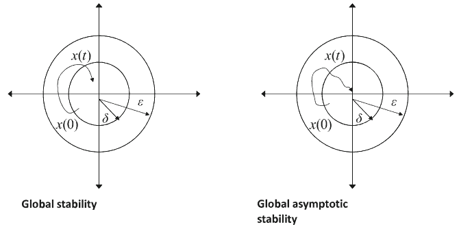
A fixed point for the system of Eq. (1.27) is called hyperbolic if none of the eigenvalues of matrix $A$ has zero real part. A hyperbolic fixed point is called a saddle if some of the eigenvalues of matrix $A$ have real parts greater than zero and the rest of the eigenvalues have real parts less than zero. If all of the eigenvalues have negative real parts then the hyperbolic fixed point is called a stable node or sink. If all of the eigenvalues have positive real parts then the hyperbolic fixed point is called an unstable node or source. If the eigenvalues are purely imaginary then one has an elliptic fixed point which is said to be a center.
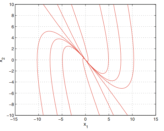
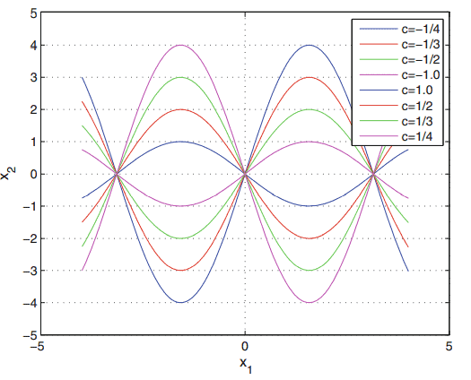
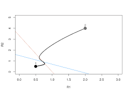
Case 1: Both eigenvalues of matrix $A$ are real and unequal, that is $\lambda_1 \neq \lambda_1 \neq 0$. For $\lambda_1<0$ and $\lambda_2<0$ the phase diagram for $z_1$ and $z_2$ is shown in Fig. 1.4. In case that $\lambda_2$ is smaller than $\lambda_1$ the term $e^{\lambda_2 t}$ decays faster than $e^{\lambda_1 t}$. For $\lambda_1>0>\lambda_2$ the phase diagram of Fig. $1.5$ is obtained.

In the latter case there are stable trajectories along eigenvector $v_1$ and unstable trajectories along eigenvector $v_2$ of matrix $A$. The stability point $(0,0)$ is said to be a saddle point.
When $\lambda_1>\lambda_2>0$ then one has the phase diagrams of Fig. 1.6.
Case 2: Complex eigenvalues:
Typical phase diagrams in the case of stable complex eigenvalues are given in Fig. 1.7.
Typical phase diagrams in the case of unstable complex eigenvalues are given in Fig. 1.8.

Typical phase diagrams in the case of imaginary eigenvalues are given in Fig. 1.9.
Case 3: Matrix $A$ has nonzero eigenvalues which are equal to each other. The associated phase diagram is given in Fig. 1.10.

金融代写|金融工程作业代写Financial Engineering代考|Saddle-Node Bifurcations of Fixed Points

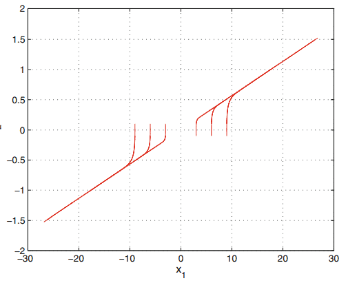
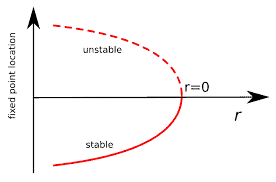
The considered dynamical system is given by $\dot{x}=\mu-x^2$. The fixed points of the system result from the condition $\dot{x}=0$ which for $\mu>0$ gives $x^*=\pm \sqrt{\mu}$. The first fixed point $x=\sqrt{\mu}$ is a stable one whereas the second fixed point $x=-\sqrt{\mu}$ is an unstable one. The phase diagram of the system is given in Fig. 1.14. Since there is one stable and one unstable fixed point the associated bifurcation (locus of the fixed points in the phase plane) will be a saddle-node one.

The bifurcations diagram is given next. The diagram shows how the fixed points of the dynamical system vary with respect to the values of parameter $\mu$. In the above case it represents a parabola in the $\mu-x$ plane as shown in Fig. 1.15.

For $\mu>0$ the dynamical system has two fixed points located at $\pm \sqrt{\mu}$. The one fixed point is stable and is associated with the upper branch of the parabola. The other fixed point is unstable and is associated with the lower branch of the parabola. The value $\mu=0$ is considered to be a bifurcation value and the point $(x, \mu)=(0,0)$ is a bifurcation point. This particular type of bifurcation where the one branch is associated with fixed points and the other branch is not associated to any fixed points is known as saddle-node bifurcation.

In pitchfork bifurcations the number of fixed points varies with respect to the values of the bifurcation parameter. The dynamical system $\dot{x}=x\left(\mu-x^2\right)$ is considered. The associated fixed points are found by the condition $\dot{x}=0$. For $\mu<0$ there is one fixed point at zero which is stable. For $\mu=0$ there is still one fixed point at zero which is still stable. For $\mu>0$ there are three fixed points, one at $x=0$, one at $x=+\sqrt{\mu}$ which is stable and one at $x=-\sqrt{\mu}$ which is also stable. The associated phase diagrams and fixed points are presented in Fig. 1.16.

金融工程代写

金融代写|金融工程作业代写Financial Engineering代考|Phase Diagrams for Linear Dynamical Systems

考虑以下自治线性系统
$$
\dot{x}=A x
$$
矩阵的特征值 $A$ 定义系统动力学。与固定点相关的一些术语如下:
方程式系统的固定点。如果没有矩阵的特征值，则 (1.27) 称为双曲线 $A$ 实部为零。如果矩阵的某些特征值 $A$ 实部大于零，其余特征值的实部小于零。如果所有特征值都具有负实部，则双曲不动点称为稳定节点或汇点。如果所有特征值都具有正实部，则双曲不动点称为不稳定节点或源。如果特征值是纯虚数，则有一个椭圆不动点，称为中心。
情况 1: 矩阵的两个特征值 $A$ 是实数且不相等的，即 $\lambda_1 \neq \lambda_1 \neq 0$. 为了 $\lambda_1<0$ 和 $\lambda_2<0$ 的相图 $z_1$ 和 $z_2$ 如图 $1.4$ 所示。万 $\lambda_2$ 小于 $\lambda_1$ 期限 $e^{\lambda_2 t}$ 衰减得比 $e^{\lambda_1 t}$. 为了 $\lambda_1>0>\lambda_2$ 图的相图。1.5获得。
在后一种情况下，沿着特征向量有稳定的轨迹 $v_1$ 和沿特征向量的不稳定轨迹 $v_2$ 矩阵的 $A$. 稳定点 $(0,0)$ 被称为鞍点。
什么时候 $\lambda_1>\lambda_2>0$ 然后是图 $1.6$ 的相图。
情况 2: 复特征值:
图 $1.7$ 给出了稳定复特征值情况下的典型相图。
图 $1.8$ 给出了不稳定复特征值情况下的典型相图。
图 $1.9$ 给出了虚本征值情况下的典型相图。
案例 3: 矩阵 $A$ 具有彼此相等的非零特征值。相关的相图如图 $1.10$ 所示。

金融代写|金融工程作业代写Financial Engineering代考|Saddle-Node Bifurcations of Fixed Points

所考虑的动力系统由下式给出 $\dot{x}=\mu-x^2$. 系统的固定点由条件产生 $\dot{x}=0$ 哪个 $\mu>0$ 给 $x^*=\pm \sqrt{\mu}$. 第一个固定点 $x=\sqrt{\mu}$ 是稳定的，而第二个不动点 $x=-\sqrt{\mu}$ 是一个不稳定的。系统的相图如图 $1.14$ 所示。由于存在一个稳定不动点和一个不稳定不动点，因此相关的分叉 (相平面中不动点的轨迹) 将是一个鞍节点分叉。
接下来给出分叉图。该图显示了动力系统的固定点如何随参数值变化 $\mu$. 在上面的例子中，它代表了一条抛物线 $\mu-x$ 平面如图 $1.15$ 所示。
为了 $\mu>0$ 动力系统有两个固定点位于 $\pm \sqrt{\mu}$. 一个固定点是稳定的并且与抛物线的上分支相关联。另一个不动点不稳定，与抛物线的下支有关。价值 $\mu=0$ 被认为是一个分叉值和点 $(x, \mu)=(0,0)$ 是分岔点。这种特殊类型的分叉称为鞍节点分叉，其中一个分支与固定点相关联，而另一个分支不与任何固定点相关联。
在干草叉分叉中，固定点的数量随分叉参数的值而变化。动力系统 $\dot{x}=x\left(\mu-x^2\right)$ 被认为。关联的固定点由条件找到 $\dot{x}=0$. 为了 $\mu<0$ 零处有一个固定点是稳定的。为了 $\mu=0$ 在零处仍有一个固定点仍然稳定。为了 $\mu>0$ 有三个固定点，一个在 $x=0$ ，一在 $x=+\sqrt{\mu}$ 这是稳定的，一个在 $x=-\sqrt{\mu}$ 这也是稳定的。相关的相图和固定点如图 $1.16$ 所示。
接下来给出分叉图。该图显示了动力系统的固定点如何随参数值变化 $\mu$. 在上面的例子中，它代表了一条抛物线 $\mu-x$ 平面如图 $1.17$ 所示。

金融代写|金融工程作业代写Financial Engineering代考请认准statistics-lab™

统计代写请认准statistics-lab™. statistics-lab™为您的留学生涯保驾护航。

金融工程代写

金融工程是使用数学技术来解决金融问题。金融工程使用计算机科学、统计学、经济学和应用数学领域的工具和知识来解决当前的金融问题，以及设计新的和创新的金融产品。

非参数统计代写

非参数统计指的是一种统计方法，其中不假设数据来自于由少数参数决定的规定模型；这种模型的例子包括正态分布模型和线性回归模型。

广义线性模型代考

广义线性模型（GLM）归属统计学领域，是一种应用灵活的线性回归模型。该模型允许因变量的偏差分布有除了正态分布之外的其它分布。

术语广义线性模型（GLM）通常是指给定连续和/或分类预测因素的连续响应变量的常规线性回归模型。它包括多元线性回归，以及方差分析和方差分析（仅含固定效应）。

有限元方法代写

有限元方法（FEM）是一种流行的方法，用于数值解决工程和数学建模中出现的微分方程。典型的问题领域包括结构分析、传热、流体流动、质量运输和电磁势等传统领域。

有限元是一种通用的数值方法，用于解决两个或三个空间变量的偏微分方程（即一些边界值问题）。为了解决一个问题，有限元将一个大系统细分为更小、更简单的部分，称为有限元。这是通过在空间维度上的特定空间离散化来实现的，它是通过构建对象的网格来实现的：用于求解的数值域，它有有限数量的点。边界值问题的有限元方法表述最终导致一个代数方程组。该方法在域上对未知函数进行逼近。[1] 然后将模拟这些有限元的简单方程组合成一个更大的方程系统，以模拟整个问题。然后，有限元通过变化微积分使相关的误差函数最小化来逼近一个解决方案。

tatistics-lab作为专业的留学生服务机构，多年来已为美国、英国、加拿大、澳洲等留学热门地的学生提供专业的学术服务，包括但不限于Essay代写，Assignment代写，Dissertation代写，Report代写，小组作业代写，Proposal代写，Paper代写，Presentation代写，计算机作业代写，论文修改和润色，网课代做，exam代考等等。写作范围涵盖高中，本科，研究生等海外留学全阶段，辐射金融，经济学，会计学，审计学，管理学等全球99%专业科目。写作团队既有专业英语母语作者，也有海外名校硕博留学生，每位写作老师都拥有过硬的语言能力，专业的学科背景和学术写作经验。我们承诺100%原创，100%专业，100%准时，100%满意。

随机分析代写

随机微积分是数学的一个分支，对随机过程进行操作。它允许为随机过程的积分定义一个关于随机过程的一致的积分理论。这个领域是由日本数学家伊藤清在第二次世界大战期间创建并开始的。

时间序列分析代写

随机过程，是依赖于参数的一组随机变量的全体，参数通常是时间。随机变量是随机现象的数量表现，其时间序列是一组按照时间发生先后顺序进行排列的数据点序列。通常一组时间序列的时间间隔为一恒定值（如1秒，5分钟，12小时，7天，1年），因此时间序列可以作为离散时间数据进行分析处理。研究时间序列数据的意义在于现实中，往往需要研究某个事物其随时间发展变化的规律。这就需要通过研究该事物过去发展的历史记录，以得到其自身发展的规律。

回归分析代写

多元回归分析渐进（Multiple Regression Analysis Asymptotics）属于计量经济学领域，主要是一种数学上的统计分析方法，可以分析复杂情况下各影响因素的数学关系，在自然科学、社会和经济学等多个领域内应用广泛。

MATLAB代写

MATLAB 是一种用于技术计算的高性能语言。它将计算、可视化和编程集成在一个易于使用的环境中，其中问题和解决方案以熟悉的数学符号表示。典型用途包括：数学和计算算法开发建模、仿真和原型制作数据分析、探索和可视化科学和工程图形应用程序开发，包括图形用户界面构建MATLAB 是一个交互式系统，其基本数据元素是一个不需要维度的数组。这使您可以解决许多技术计算问题，尤其是那些具有矩阵和向量公式的问题，而只需用 C 或 Fortran 等标量非交互式语言编写程序所需的时间的一小部分。MATLAB 名称代表矩阵实验室。MATLAB 最初的编写目的是提供对由 LINPACK 和 EISPACK 项目开发的矩阵软件的轻松访问，这两个项目共同代表了矩阵计算软件的最新技术。MATLAB 经过多年的发展，得到了许多用户的投入。在大学环境中，它是数学、工程和科学入门和高级课程的标准教学工具。在工业领域，MATLAB 是高效研究、开发和分析的首选工具。MATLAB 具有一系列称为工具箱的特定于应用程序的解决方案。对于大多数 MATLAB 用户来说非常重要，工具箱允许您学习和应用专业技术。工具箱是 MATLAB 函数（M 文件）的综合集合，可扩展 MATLAB 环境以解决特定类别的问题。可用工具箱的领域包括信号处理、控制系统、神经网络、模糊逻辑、小波、仿真等。

R语言代写	问卷设计与分析代写
PYTHON代写	回归分析与线性模型代写
MATLAB代写	方差分析与试验设计代写
STATA代写	机器学习/统计学习代写
SPSS代写	计量经济学代写
EVIEWS代写	时间序列分析代写
EXCEL代写	深度学习代写
SQL代写	各种数据建模与可视化代写

金融代写|金融工程作业代写Financial Engineering代考|ICEFE2022

Posted on 2023年2月10日2023年2月10日 by statistics-lab

如果你也在怎样代写金融工程Financial Engineering这个学科遇到相关的难题，请随时右上角联系我们的24/7代写客服。

我们提供的金融工程Financial Engineering及其相关学科的代写，服务范围广, 其中包括但不限于:

Statistical Inference 统计推断
Statistical Computing 统计计算
Advanced Probability Theory 高等概率论
Advanced Mathematical Statistics 高等数理统计学
(Generalized) Linear Models 广义线性模型
Statistical Machine Learning 统计机器学习
Longitudinal Data Analysis 纵向数据分析
Foundations of Data Science 数据科学基础

金融代写|金融工程作业代写Financial Engineering代考|ICEFE2022

金融代写|金融工程作业代写Financial Engineering代考|Lyapunov Stability Approach

The Lyapunov method analyzes the stability of a dynamical system without the need to compute explicitly the trajectories of the state vector $x=\left[x_1, x_2, \cdots, x_n\right]^T$.
Theorem: The system described by the relation $\dot{x}=f(x)$ is asymptotically stable in the vicinity of the equilibrium $x_0=0$ if there is a function $V(x)$ such that
(i) $V(x)$ to be continuous and to have a continuous first order derivative at $x_0$
(ii) $V(x)>0$ if $x \neq 0$ and $V(0)=0$
(iii) $\dot{V}(x)<0, \forall x \neq 0$.
The Lyapunov function is usually chosen to be a quadratic (and thus positive) energy function of the system however there in no systematic method to define it.

Assume now, that $\dot{x}=f(x)$ and $x_0=0$ is the equilibrium. Then the system is globally asymptotically stable if for every $\varepsilon>0, \exists \delta(\varepsilon)>0$, such that if $|x(0)|<\delta$ then $|x(t)|<\varepsilon, \forall t \geq 0$.

This means that if the state vector of the system starts in a disc of radius $\delta$ then as time advances it will remain in the disc of radius $\varepsilon$, as shown in Fig. 1.3. Moreover, if $\lim _{t \rightarrow \infty}|x(t)|=x_0=0$ then the system is globally asymptotically stable.
Example 1: Consider the system
$$
\begin{gathered}
\dot{x}_1=x_2 \
\dot{x}_2=-x_1-x_3^2
\end{gathered}
$$
The following Lyapunov function is defined
$$
V(x)-x_1^2+x_2^2
$$

The equilibrium point is $\left(x_1=0, x_2=0\right)$. It holds that $V(x)>0 \forall\left(x_1, x_2\right) \neq(0,0)$ and $V(x)=0$ for $\left(x_1, x_2\right)=(0,0)$. Moreover, it holds
$$
\begin{gathered}
\dot{V}(x)=2 x_1 \dot{x}1+2 x_2 \dot{x}_2=2 x_1 x_2+2 x_2\left(-x_1-x_2^3\right) \Rightarrow \ \dot{V}(x)=-2 x_2^4<0 \forall\left(x_1, x_2\right) \neq(0,0) \end{gathered} $$ Therefore, the system is asymptotically stable and $\lim {t \rightarrow \infty}\left(x_1, x_2\right)=(0,0)$.

金融代写|金融工程作业代写Financial Engineering代考|Local Stability Properties of a Nonlinear Model

Local stability of a nonlinear model can be studied round the associated equilibria. Local linearization can be performed round equilibria, using the set of differential equations that describe the nonlinear model $\dot{x}=h(x)$ and performing Taylor series expansion, that is $\dot{x}=h(x) \Rightarrow \dot{x}=\left.h\left(x_0\right)\right|_{x_0}+\nabla_x h\left(x-x_0\right)+\cdots$.
The nonlinear model is taken to have the generic form
$$
\left(\begin{array}{l}
\dot{x}_1 \
\dot{x}_2
\end{array}\right)=\left(\begin{array}{l}
f\left(x_1, x_2\right) \
g\left(x_1, x_2\right)
\end{array}\right)
$$
where $f\left(x_1, x_2\right)=2 x_1+x_2^2$ and $g\left(x_1, x_2\right)=x_1^2+2 x_2$. The fixed points of this model are computed from the condition $\dot{x}_1=0$ and $\dot{x}_2=0$. Using these relations one finds the equilibria $\left(x_1^, x_2^\right)=(0,0)$ and $\left(x_1^, x_2^\right)=(0,0)$
The Jacobian matrix $\nabla_x h=M$ is given by
$$
M=\left(\begin{array}{ll}
\frac{\partial f}{\partial x_1} & \frac{\partial f}{\partial x_2} \
\frac{\partial g}{\partial x_1} & \frac{\partial g}{\partial x_2}
\end{array}\right)
$$
which results into the matrix
$$
J=\left(\begin{array}{cc}
2 & 2 x_2 \
2 x_1 & 2
\end{array}\right)
$$
The eigenvalues of matrix $M$ define stability round fixed points (stable or unstable fixed point). To this end, one has to find the roots of the associated characteristic polynomial that is given by $\operatorname{det}(\lambda I-J)=0$ where $I$ is the identity matrix.

金融工程代写

金融代写|金融工程作业代写Financial Engineering代考|Lyapunov Stability Approach

Lyapunov 方法分析动力系统的稳定性，无需显式计算状态向量的轨迹
$$
x=\left[x_1, x_2, \cdots, x_n\right]^T \text {. }
$$
定理: 由关系描述的系统 $\dot{x}=f(x)$ 在平衡点附近渐近稳定 $x_0=0$ 如果有函数 $V(x)$ 这样
(i) $V(x)$ 是连续的，并且有一个连续的一阶导数在 $x_0$
(二) $V(x)>0$ 如果 $x \neq 0$ 和 $V(0)=0$
(三) $\dot{V}(x)<0, \forall x \neq 0$. Lyapunov 函数通常被选择为系统的二次 (因此是正) 能量函数，但是没有系统的方法来定义它。现在假设， $\dot{x}=f(x)$ 和 $x_0=0$ 是平衡点。那么系统是全局渐近稳定的如果对于每个 $\varepsilon>0, \exists \delta(\varepsilon)>0$, 这样如果 $|x(0)|<\delta$ 然后 $|x(t)|<\varepsilon, \forall t \geq 0$. 这意味着如果系统的状态向量开始于半径为 $\delta$ 然后随着时间的推移它将保留在半径的圆盘中 $\varepsilon$ ，如图1.3所示。此外，如果 $\lim _{t \rightarrow \infty}|x(t)|=x_0=0$ 那么系统是全局渐近稳定的。示例 1：考虑系统 $$ \dot{x}_1=x_2 \dot{x}_2=-x_1-x_3^2 $$ 定义了以下 Lyapunov 函数 $$ V(x)-x_1^2+x_2^2 $$ 平衡点是 $\left(x_1=0, x_2=0\right)$. 它认为 $V(x)>0 \forall\left(x_1, x_2\right) \neq(0,0)$ 和 $V(x)=0$ 为了 $\left(x_1, x_2\right)=(0,0)$. 此外，它持有
$$
\dot{V}(x)=2 x_1 \dot{x} 1+2 x_2 \dot{x}_2=2 x_1 x_2+2 x_2\left(-x_1-x_2^3\right) \Rightarrow \dot{V}(x)=-2 x_2^4<0 \forall\left(x_1, x_2\right)
$$
因此，系统斩近稳定且 $\lim t \rightarrow \infty\left(x_1, x_2\right)=(0,0)$.

金融代写|金融工程作业代写Financial Engineering代考|Local Stability Properties of a Nonlinear Model

非线性模型的局部稳定性可以围绕相关平衡进行研究。可以使用描述非线性模型的微分方程组在循环平衡中执行局部线性化 $\dot{x}=h(x)$ 并进行泰勒级数展开，即 $\dot{x}=h(x) \Rightarrow \dot{x}=\left.h\left(x_0\right)\right|{x_0}+\nabla_x h\left(x-x_0\right)+\cdots$ 非线性模型采用一般形式 $$ \left(\dot{x}_1 \dot{x}_2\right)=\left(f\left(x_1, x_2\right) g\left(x_1, x_2\right)\right) $$ 在哪里 $f\left(x_1, x_2\right)=2 x_1+x_2^2$ 和 $g\left(x_1, x_2\right)=x_1^2+2 x_2$. 该模型的固定点是根据条件计算的 $\dot{x}_1=0$ 和 $\dot{x}_2=0$. 使用这些关系可以找到平衡点 $\bigcup$ |left $\left(x{-} 1 \wedge, x_{-} 2 \wedge r i g h t\right)=(0,0)$ 和
left $\left(x_{-} 1 \wedge, x_{-} _2 \wedge\right.$ right $)=(0,0)$
雅可比矩阵 $\nabla_x h=M$ 是 (谁) 给的
$$
M=\left(\begin{array}{llll}
\frac{\partial f}{\partial x_1} & \frac{\partial f}{\partial x_2} & \frac{\partial g}{\partial x_1} & \frac{\partial g}{\partial x_2}
\end{array}\right)
$$
结果进入矩阵
$$
J=\left(\begin{array}{lll}
2 & 2 x_2 2 x_1 & 2
\end{array}\right)
$$
矩阵的特征值 $M$ 定义围绕固定点的稳定性 (稳定或不稳定的固定点)。为此，必须找到由下式给出的相关特征多项式的根 $\operatorname{det}(\lambda I-J)=0$ 在哪里 $I$ 是单位矩阵。

统计代写请认准statistics-lab™. statistics-lab™为您的留学生涯保驾护航。

金融工程代写

非参数统计代写

非参数统计指的是一种统计方法，其中不假设数据来自于由少数参数决定的规定模型；这种模型的例子包括正态分布模型和线性回归模型。

广义线性模型代考

广义线性模型（GLM）归属统计学领域，是一种应用灵活的线性回归模型。该模型允许因变量的偏差分布有除了正态分布之外的其它分布。

有限元方法代写

随机分析代写

时间序列分析代写

回归分析代写

MATLAB代写

R语言代写	问卷设计与分析代写
PYTHON代写	回归分析与线性模型代写
MATLAB代写	方差分析与试验设计代写
STATA代写	机器学习/统计学习代写
SPSS代写	计量经济学代写
EVIEWS代写	时间序列分析代写
EXCEL代写	深度学习代写
SQL代写	各种数据建模与可视化代写

金融代写|金融工程作业代写Financial Engineering代考|Best107

Posted on 2023年2月10日2023年2月10日 by statistics-lab

如果你也在怎样代写金融工程Financial Engineering这个学科遇到相关的难题，请随时右上角联系我们的24/7代写客服。

我们提供的金融工程Financial Engineering及其相关学科的代写，服务范围广, 其中包括但不限于:

Statistical Inference 统计推断
Statistical Computing 统计计算
Advanced Probability Theory 高等概率论
Advanced Mathematical Statistics 高等数理统计学
(Generalized) Linear Models 广义线性模型
Statistical Machine Learning 统计机器学习
Longitudinal Data Analysis 纵向数据分析
Foundations of Data Science 数据科学基础

金融代写|金融工程作业代写Financial Engineering代考|Best107

金融代写|金融工程作业代写Financial Engineering代考|Characteristics of the Dynamics of Nonlinear Systems

Main features characterizing the stability of nonlinear dynamical systems are defined as follows [121, 274]:

Finite escape time: It is the finite time within which the state-vector of the nonlinear system converges to infinity.
Multiple isolated equilibria: A linear system can have only one equilibrium to which converges the state vector of the system in steady-state. A nonlinear system can have more than one isolated equilibria (fixed points). Depending on the initial state of the system, in steady-state the state vector of the system can converge to one of these equilibria.
Limit cycles: For a linear system to exhibit oscillations it must have eigenvalues on the imaginary axis. The amplitude of the oscillations depends on initial conditions. In nonlinear systems one may have oscillations of constant amplitude and frequency, which do not depend on initial conditions. This type of oscillations is known as limit cycles.
Sub-harmonic, harmonic and almost periodic oscillations: A stable linear system under periodic input produces an output of the same frequency. A nonlinear system,

under periodic excitation can generate oscillations with frequencies which are several times smaller (subharmonic) or multiples of the frequency of the input (harmonic). It may also generate almost periodic oscillations with frequencies which are not necessarily multiples of a basis frequency (almost periodic oscillations).

Chaos: A nonlinear system in steady-state can exhibit a behavior which is not characterized as equilibrium, periodic oscillation or almost periodic oscillation. This behavior is characterized as chaos. As time advances the behavior of the system changes in a random-like manner, and this depends on the initial conditions. Although the dynamic system is deterministic it exhibits randomness in the way it evolves in time.
Multiple modes of behavior: It is possible the same dynamical system to exhibit simultaneously more than one of the aforementioned characteristics (1)-(5). Thus, a system without external excitation may exhibit simultaneously more than one limit cycles. A system receiving a periodic external input may exhibit harmonic or subharmonic oscillations, or an even more complex behavior in steady state which depends on the amplitude and frequency of the excitation.

金融代写|金融工程作业代写Financial Engineering代考|Computation of Isoclines

An autonomous second order system is described by two differential equations of the form
$$
\begin{aligned}
& \dot{x}_1=f_1\left(x_1, x_2\right) \
& \dot{x}_2=f_2\left(x_1, x_2\right)
\end{aligned}
$$
The method of the isoclines consists of computing the slope (ratio) between $f_2$ and $f_1$ for every point of the trajectory of the state vector $\left(x_1, x_2\right)$.
$$
s(x)=\frac{f_2\left(x_1, x_2\right)}{f_1\left(x_1, x_2\right)}
$$
The case $s(x)=c$ describes a curve in the $x_1-x_2$ plane along which the trajectories $\dot{x}_1=f_1\left(x_1, x_2\right)$ and $\dot{x}_2=f_2\left(x_1, x_2\right)$ have a constant slope.

The curve $s(x)=c$ is drawn in the $x_1-x_2$ plane and along this curve one also draws small linear segments of length $c$. The curve $s(x)=c$ is known as isocline. The direction of these small linear segments is according to the sign of the ratio $f_2\left(x_1, x_2\right) / f_1\left(x_1, x_2\right)$.
Example 1:
The following simplified nonlinear dynamical system is considered
$$
\begin{gathered}
\dot{x}_1=x_2 \
\dot{x}_2=-\sin \left(x_1\right)
\end{gathered}
$$

The slope $s(x)$ is given by the relation
$$
s(x)=\frac{f_2\left(x_1, x_2\right)}{f_1\left(x_1, x_2\right)} \Rightarrow s(x)=-\frac{s i n\left(x_2\right)}{x_2}
$$
Setting $s(x)=c$ it holds that the isoclines are given by the relation
$$
x_2=-\frac{1}{c} \sin \left(x_1\right)
$$
For different values of $c$ one has the following isoclines diagram depicted in Fig. 1.1. Example 2:

The following oscillator model is considered, being free of friction and with statespace equations
$$
\begin{gathered}
\dot{x}_1=x_2 \
\dot{x}_2=-0.5 x_2-\sin \left(x_1\right)
\end{gathered}
$$

金融工程代写

金融代写|金融工程作业代写Financial Engineering代考|Characteristics of the Dynamics of Nonlinear Systems

表征非线性动力系统稳定性的主要特征定义如下 [121, 274]：

有限逃逸时间：是非线性系统的状态向量收敛到无穷大的有限时间。
多重孤立平衡：一个线性系统只能有一个平衡点，该平衡点收敛于稳态系统的状态向量。一个非线性系统可以有多个孤立的平衡点（不动点）。根据系统的初始状态，在稳态下，系统的状态向量可以收敛到这些平衡点之一。
极限环：对于表现出振荡的线性系统，它必须在虚轴上具有特征值。振荡的幅度取决于初始条件。在非线性系统中，可能存在幅度和频率恒定的振荡，不依赖于初始条件。这种类型的振荡被称为极限环。
次谐波、谐波和几乎周期性振荡：在周期性输入下稳定的线性系统会产生相同频率的输出。一个非线性系统，

在周期性激励下会产生频率比输入频率小几倍（次谐波）或数倍（谐波）的振荡。它还可能产生几乎周期性的振荡，其频率不一定是基频的倍数（几乎周期性振荡）。

混沌：处于稳态的非线性系统可能表现出一种不具有平衡、周期性振荡或几乎周期性振荡特征的行为。这种行为的特点是混乱。随着时间的推移，系统的行为会以类似随机的方式发生变化，这取决于初始条件。尽管动态系统是确定性的，但它随时间演化的方式表现出随机性。
多种行为模式：同一动力系统可能同时表现出上述特征 (1)-(5) 中的一个以上。因此，没有外部激励的系统可能同时表现出多个极限循环。接收周期性外部输入的系统可能会表现出谐波或次谐波振荡，或者在稳态下表现出更复杂的行为，这取决于激励的幅度和频率。

金融代写|金融工程作业代写Financial Engineering代考|Computation of Isoclines

自治二阶系统由以下形式的两个微分方程描述
$$
\dot{x}_1=f_1\left(x_1, x_2\right) \quad \dot{x}_2=f_2\left(x_1, x_2\right)
$$
等斜线的方法包括计算之间的斜率 (比率) $f_2$ 和 $f_1$ 对于状态向量轨迹的每一点 $\left(x_1, x_2\right)$.
$$
s(x)=\frac{f_2\left(x_1, x_2\right)}{f_1\left(x_1, x_2\right)}
$$
案子 $s(x)=c$ 描述了一条曲线 $x_1-x_2$ 轨迹沿着的平面 $\dot{x}_1=f_1\left(x_1, x_2\right)$ 和 $\dot{x}_2=f_2\left(x_1, x_2\right)$ 有一个恒定的斜率。
曲线 $s(x)=c$ 被绘制在 $x_1-x_2$ 平面并沿着这条曲线也绘制了长度的小线性段 $c$. 曲线 $s(x)=c$ 被称为等倾角。这些小线段的方向是根据比率的符号 $f_2\left(x_1, x_2\right) / f_1\left(x_1, x_2\right)$. 示例 1:
考虑以下简化的非线性动力系统
$$
\dot{x}_1=x_2 \dot{x}_2=-\sin \left(x_1\right)
$$
斜坡 $s(x)$ 由关系给出
$$
s(x)=\frac{f_2\left(x_1, x_2\right)}{f_1\left(x_1, x_2\right)} \Rightarrow s(x)=-\frac{\sin \left(x_2\right)}{x_2}
$$
环境 $s(x)=c$ 它认为等斜线由关系给出
$$
x_2=-\frac{1}{c} \sin \left(x_1\right)
$$
对于不同的值 $c$ 一个具有以下图 $1.1$ 中描绘的等倾线图。示例 2 :
考虑以下振荡器模型，无摩擦且具有状态空间方程
$$
\dot{x}_1=x_2 \dot{x}_2=-0.5 x_2-\sin \left(x_1\right)
$$

统计代写请认准statistics-lab™. statistics-lab™为您的留学生涯保驾护航。

金融工程代写

非参数统计代写

非参数统计指的是一种统计方法，其中不假设数据来自于由少数参数决定的规定模型；这种模型的例子包括正态分布模型和线性回归模型。

广义线性模型代考

广义线性模型（GLM）归属统计学领域，是一种应用灵活的线性回归模型。该模型允许因变量的偏差分布有除了正态分布之外的其它分布。

有限元方法代写

随机分析代写

时间序列分析代写

回归分析代写

MATLAB代写

R语言代写	问卷设计与分析代写
PYTHON代写	回归分析与线性模型代写
MATLAB代写	方差分析与试验设计代写
STATA代写	机器学习/统计学习代写
SPSS代写	计量经济学代写
EVIEWS代写	时间序列分析代写
EXCEL代写	深度学习代写
SQL代写	各种数据建模与可视化代写

金融代写|金融工程作业代写Financial Engineering代考|BE953

Posted on 2022年7月21日2023年10月17日 by statistics-lab

如果你也在怎样代写金融工程Financial Engineering这个学科遇到相关的难题，请随时右上角联系我们的24/7代写客服。

我们提供的金融工程Financial Engineering及其相关学科的代写，服务范围广, 其中包括但不限于:

Statistical Inference 统计推断
Statistical Computing 统计计算
Advanced Probability Theory 高等概率论
Advanced Mathematical Statistics 高等数理统计学
(Generalized) Linear Models 广义线性模型
Statistical Machine Learning 统计机器学习
Longitudinal Data Analysis 纵向数据分析
Foundations of Data Science 数据科学基础

金融代写|金融工程作业代写Financial Engineering代考|Local Stability Properties of a Nonlinear Model

Local stability of a nonlinear model can be studied round the associated equilibria. Local linearization can be performed round equilibria, using the set of differential equations that describe the nonlinear model $\dot{x}=h(x)$ and performing Taylor series expansion, that is $\dot{x}=h(x) \Rightarrow \dot{x}=\left.h\left(x_{0}\right)\right|{x{0}}+\nabla_{x} h\left(x-x_{0}\right)+\cdots$.
The nonlinear model is taken to have the generic form
$$
\left(\begin{array}{l}
\dot{x}{1} \ \dot{x}{2}
\end{array}\right)=\left(\begin{array}{l}
f\left(x_{1}, x_{2}\right) \
g\left(x_{1}, x_{2}\right)
\end{array}\right)
$$
where $f\left(x_{1}, x_{2}\right)=2 x_{1}+x_{2}^{2}$ and $g\left(x_{1}, x_{2}\right)=x_{1}^{2}+2 x_{2}$. The fixed points of this model are computed from the condition $\dot{x}{1}=0$ and $\dot{x}{2}=0$. Using these relations one finds the equilibria $\left(x_{1}^{}, x_{2}^{}\right)=(0,0)$ and $\left(x_{1}^{}, x_{2}^{}\right)=(0,0)$
The Jacobian matrix $\nabla_{x} h=M$ is given by
$$
M=\left(\begin{array}{ll}
\frac{\partial f}{\partial x_{1}} & \frac{\partial f}{\partial x_{2}} \
\frac{\partial g}{\partial x_{1}} & \frac{\partial g}{\partial x_{2}}
\end{array}\right)
$$
which results into the matrix
$$
J=\left(\begin{array}{cc}
2 & 2 x_{2} \
2 x_{1} & 2
\end{array}\right)
$$

金融代写|金融工程作业代写Financial Engineering代考|Phase Diagrams for Linear Dynamical Systems

The following autonomous linear system is considered
$$
\dot{x}=A x
$$
The eigenvalues of matrix $A$ define the system dynamics. Some terminology associated with fixed points is as follows:

A fixed point for the system of Eq. (1.27) is called hyperbolic if none of the eigenvalues of matrix $A$ has zero real part. A hyperbolic fixed point is called a saddle if some of the eigenvalues of matrix $A$ have real parts greater than zero and the rest of the eigenvalues have real parts less than zero. If all of the eigenvalues have negative real parts then the hyperbolic fixed point is called a stable node or sink. If all of the eigenvalues have positive real parts then the hyperbolic fixed point is called an unstable node or source. If the eigenvalues are purely imaginary then one has an elliptic fixed point which is said to be a center.
Case 1: Both eigenvalues of matrix $A$ are real and unequal, that is $\lambda_{1} \neq \lambda_{1} \neq 0$. For $\lambda_{1}<0$ and $\lambda_{2}<0$ the phase diagram for $z_{1}$ and $z_{2}$ is shown in Fig. 1.4. In case that $\lambda_{2}$ is smaller than $\lambda_{1}$ the term $e^{\lambda_{2} t}$ decays faster than $e^{\lambda_{1} t}$. For $\lambda_{1}>0>\lambda_{2}$ the phase diagram of Fig. $1.5$ is obtained.

金融工程代写

金融代写|金融工程作业代写Financial Engineering代考|Local Stability Properties of a Nonlinear Model

非线性模型的局部稳定性可以围绕相关的平衡来研究。使用描述非线性模型的微分方程组，可以围绕平衡执行局部线性化 $\dot{x}=h(x)$ 并执行泰勒级数展开，即 $\dot{x}=h(x) \Rightarrow \dot{x}=h\left(x_{0}\right) \mid x 0+\nabla_{x} h\left(x-x_{0}\right)+\cdots$. 非线性模型被取为具有一般形式
$$
(\dot{x} 1 \dot{x} 2)=\left(f\left(x_{1}, x_{2}\right) g\left(x_{1}, x_{2}\right)\right)
$$
在哪里 $f\left(x_{1}, x_{2}\right)=2 x_{1}+x_{2}^{2}$ 和 $g\left(x_{1}, x_{2}\right)=x_{1}^{2}+2 x_{2}$. 该模型的不动点是根据条件计算的 $\dot{x} 1=0$ 和 $\dot{x} 2=0$. 使用这些关系可以找到平衡 $\left(x_{1}, x_{2}\right)=(0,0)$ 和 $\left(x_{1}, x_{2}\right)=(0,0)$ 雅可比矩阵 $\nabla_{x} h=M$ 是 (谁) 给的
$$
M=\left(\begin{array}{lll}
\frac{\partial f}{\partial x_{1}} \quad \frac{\partial f}{\partial x_{2}} & \frac{\partial g}{\partial x_{1}} & \frac{\partial g}{\partial x_{2}}
\end{array}\right)
$$
这导致矩阵

金融代写|金融工程作业代写Financial Engineering代考|Phase Diagrams for Linear Dynamical Systems

考虑以下自治线性系统
$$
\dot{x}=A x
$$
矩阵的特征值 $A$ 定义系统动力学。与固定点相关的一些术语如下:
方程系统的不动点。如果矩阵没有任何特征值，则称 (1.27) 为双曲线 $A$ 实部为零。如果矩阵的某些特征值，则双曲不动点称为鞍 $A$ 实部大于零，其余特征值的实部小于零。如果所有特征值都具有负实部，则双曲不动点称为稳定节点或汇点。如果所有特征值都具有正实部，则双曲不动点称为不稳定节点或源。如果特征值是纯虚数，则有一个椭圆不动点，称为中心。
案例1: 矩阵的两个特征值 $A$ 是真实的和不平等的，即 $\lambda_{1} \neq \lambda_{1} \neq 0$. 为了 $\lambda_{1}<0$ 和 $\lambda_{2}<0$ 相图 $z_{1}$ 和 $z_{2}$ 如图 $1.4$ 所示。万一 $\lambda_{2}$ 小于 $\lambda_{1}$ 期限 $e^{\lambda_{2} t}$ 衰减速度比 $e^{\lambda_{1} t}$. 为了 $\lambda_{1}>0>\lambda_{2}$ 图的相图1.5获得。

统计代写请认准statistics-lab™. statistics-lab™为您的留学生涯保驾护航。

金融工程代写

非参数统计代写

非参数统计指的是一种统计方法，其中不假设数据来自于由少数参数决定的规定模型；这种模型的例子包括正态分布模型和线性回归模型。

广义线性模型代考

广义线性模型（GLM）归属统计学领域，是一种应用灵活的线性回归模型。该模型允许因变量的偏差分布有除了正态分布之外的其它分布。

有限元方法代写

随机分析代写

时间序列分析代写

回归分析代写

MATLAB代写

R语言代写	问卷设计与分析代写
PYTHON代写	回归分析与线性模型代写
MATLAB代写	方差分析与试验设计代写
STATA代写	机器学习/统计学习代写
SPSS代写	计量经济学代写
EVIEWS代写	时间序列分析代写
EXCEL代写	深度学习代写
SQL代写	各种数据建模与可视化代写

金融代写|金融工程作业代写Financial Engineering代考|ICEFE 2022

Posted on 2022年7月21日2022年7月21日 by statistics-lab

如果你也在怎样代写金融工程Financial Engineering这个学科遇到相关的难题，请随时右上角联系我们的24/7代写客服。

我们提供的金融工程Financial Engineering及其相关学科的代写，服务范围广, 其中包括但不限于:

Statistical Inference 统计推断
Statistical Computing 统计计算
Advanced Probability Theory 高等概率论
Advanced Mathematical Statistics 高等数理统计学
(Generalized) Linear Models 广义线性模型
Statistical Machine Learning 统计机器学习
Longitudinal Data Analysis 纵向数据分析
Foundations of Data Science 数据科学基础

金融代写|金融工程作业代写Financial Engineering代考|The Phase Diagram

One can consider the following nonlinear model with the two state variables, $V$ and $\eta$. The dynamics of this model can be written as
$$
\begin{aligned}
\frac{d V}{d t} &=f(V, t) \
\frac{d \eta}{d t} &=g(V, \eta)
\end{aligned}
$$
The phase diagram consists of the points on the trajectories of the solution of the associated differential equation, i.e. $\left(V\left(t_{k}\right), \eta\left(t_{k}\right)\right)$.

At a fixed point or equilibrium it holds $f\left(V_{R}, \eta_{R}\right)=0$ and $g\left(V_{R}, \eta_{R}\right)=0$. The closed trajectories are associated with periodic solutions. If there are closed trajectories then $\exists T>0$ such that $\left(V\left(t_{k}\right), \eta\left(t_{k}\right)\right)=\left(V\left(t_{k}+T\right), \eta\left(t_{k}+T\right)\right)$.

Another useful parameter is the nullclines. The $V$-nullcline is characterized by the relation $\dot{V}=f(V, \eta)=0$. The $\eta$-nullcline is characterized by the relation $\dot{\eta}=g(V, \eta)=0$. The fixed points (or equilibria) are found on the intersection of nullclines.

金融代写|金融工程作业代写Financial Engineering代考|Lyapunov Stability Approach

The Lyapunov method analyzes the stability of a dynamical system without the need to compute explicitly the trajectories of the state vector $x=\left[x_{1}, x_{2}, \cdots, x_{n}\right]^{T}$.
Theorem: The system described by the relation $\dot{x}=f(x)$ is asymptotically stable in the vicinity of the equilibrium $x_{0}=0$ if there is a function $V(x)$ such that
(i) $V(x)$ to be continuous and to have a continuous first order derivative at $x_{0}$
(ii) $V(x)>0$ if $x \neq 0$ and $V(0)=0$
(iii) $\dot{V}(x)<0, \forall x \neq 0$.
The Lyapunov function is usually chosen to be a quadratic (and thus positive) energy function of the system however there in no systematic method to define it.

Assume now, that $\dot{x}=f(x)$ and $x_{0}=0$ is the equilibrium. Then the system is globally asymptotically stable if for every $\varepsilon>0, \exists \delta(\varepsilon)>0$, such that if $|x(0)|<\delta$ then $|x(t)|<\varepsilon, \forall t \geq 0$.

This means that if the state vector of the system starts in a disc of radius $\delta$ then as time advances it will remain in the disc of radius $\varepsilon$, as shown in Fig. 1.3. Moreover, if $\lim {t \rightarrow \infty}|x(t)|=x{0}=0$ then the system is globally asymptotically stable.
Example 1: Consider the system
$$
\begin{gathered}
\dot{x}{1}=x{2} \
\dot{x}{2}=-x{1}-x_{3}^{2}
\end{gathered}
$$
The following Lyapunov function is defined
$$
V(x)=x_{1}^{2}+x_{2}^{2}
$$

金融工程代写

金融代写|金融工程作业代写Financial Engineering代考|The Phase Diagram

可以考虑以下具有两个状态变量的非线性模型， $V$ 和 $\eta$. 该模型的动力学可以写为
$$
\frac{d V}{d t}=f(V, t) \frac{d \eta}{d t} \quad=g(V, \eta)
$$
相图由相关微分方程解的轨迹上的点组成，即 $\left(V\left(t_{k}\right), \eta\left(t_{k}\right)\right)$.
在固定点或平衡点，它保持 $f\left(V_{R}, \eta_{R}\right)=0$ 和 $g\left(V_{R}, \eta_{R}\right)=0$. 闭合轨迹与周期解相关联。如果有封闭的轨迹，那么 $\exists T>0$ 这样 $\left(V\left(t_{k}\right), \eta\left(t_{k}\right)\right)=\left(V\left(t_{k}+T\right), \eta\left(t_{k}+T\right)\right)$.
另一个有用的参数是 nullclines。这 $V$-nullcline 的特征是关系 $\dot{V}=f(V, \eta)=0$. 这 $\eta$-nullcline 的特征是关系 $\dot{\eta}=g(V, \eta)=0$. 在零斜线的交点上找到不动点 (或平衡点)。

金融代写|金融工程作业代写Financial Engineering代考|Lyapunov Stability Approach

Lyapunov 方法无需明确计算状态向量的轨迹即可分析动力系统的稳定性 $x=\left[x_{1}, x_{2}, \cdots, x_{n}\right]^{T}$. 定理: 由关系描述的系统 $\dot{x}=f(x)$ 在平衡点附近是渐近稳定的 $x_{0}=0$ 如果有功能 $V(x)$ 这样 (i) $V(x)$ 是连续的并且在处具有连续的一阶导数 $x_{0}$
(二) $V(x)>0$ 如果 $x \neq 0$ 和 $V(0)=0$
$\Leftrightarrow \dot{V}(x)<0, \forall x \neq 0$. Lyapunov 函数通常被选择为系统的二次 (因此是正) 能量函数，但是没有系统的方法来定义它。现在假设，那 $\dot{x}=f(x)$ 和 $x_{0}=0$ 是均衡。那么系统是全局渐近稳定的，如果对于每个 $\varepsilon>0, \exists \delta(\varepsilon)>0$, 这样如果 $|x(0)|<\delta$ 然后 $|x(t)|<\varepsilon, \forall t \geq 0$.
这意味責如果系统的状态向量开始于一个半径为 $\delta$ 然后随着时间的推移，它将留在半径的圆盘中 $\varepsilon$ ，如图 $1.3$ 所示。此外，如果 $\lim t \rightarrow \infty|x(t)|=x 0=0$ 那么系统是全局渐近稳定的。
示例 1：考虑系统
$$
\dot{x} 1=x 2 \dot{x} 2=-x 1-x_{3}^{2}
$$
定义以下 Lyapunov 函数
$$
V(x)=x_{1}^{2}+x_{2}^{2}
$$

统计代写请认准statistics-lab™. statistics-lab™为您的留学生涯保驾护航。

金融工程代写

非参数统计代写

非参数统计指的是一种统计方法，其中不假设数据来自于由少数参数决定的规定模型；这种模型的例子包括正态分布模型和线性回归模型。

广义线性模型代考

广义线性模型（GLM）归属统计学领域，是一种应用灵活的线性回归模型。该模型允许因变量的偏差分布有除了正态分布之外的其它分布。

有限元方法代写

随机分析代写

时间序列分析代写

回归分析代写

MATLAB代写

R语言代写	问卷设计与分析代写
PYTHON代写	回归分析与线性模型代写
MATLAB代写	方差分析与试验设计代写
STATA代写	机器学习/统计学习代写
SPSS代写	计量经济学代写
EVIEWS代写	时间序列分析代写
EXCEL代写	深度学习代写
SQL代写	各种数据建模与可视化代写

金融代写|金融工程作业代写Financial Engineering代考|Best 107

Posted on 2022年7月21日2022年7月21日 by statistics-lab

如果你也在怎样代写金融工程Financial Engineering这个学科遇到相关的难题，请随时右上角联系我们的24/7代写客服。

我们提供的金融工程Financial Engineering及其相关学科的代写，服务范围广, 其中包括但不限于:

Statistical Inference 统计推断
Statistical Computing 统计计算
Advanced Probability Theory 高等概率论
Advanced Mathematical Statistics 高等数理统计学
(Generalized) Linear Models 广义线性模型
Statistical Machine Learning 统计机器学习
Longitudinal Data Analysis 纵向数据分析
Foundations of Data Science 数据科学基础

金融代写|金融工程作业代写Financial Engineering代考|Characteristics of the Dynamics of Nonlinear Systems

Main features characterizing the stability of nonlinear dynamical systems are defined as follows [121, 274]:

Finite escape time: It is the finite time within which the state-vector of the nonlinear system converges to infinity.
Multiple isolated equilibria: A linear system can have only one equilibrium to which converges the state vector of the system in steady-state. A nonlinear system can have more than one isolated equilibria (fixed points). Depending on the initial state of the system, in steady-state the state vector of the system can converge to one of these equilibria.
Limit cycles: For a linear system to exhibit oscillations it must have eigenvalues on the imaginary axis. The amplitude of the oscillations depends on initial conditions. In nonlinear systems one may have oscillations of constant amplitude and frequency, which do not depend on initial conditions. This type of oscillations is known as limit cycles.
Sub-harmonic, harmonic and almost periodic oscillations: A stable linear system under periodic input produces an output of the same frequency. A nonlinear system,

Chaos: A nonlinear system in steady-state can exhibit a behavior which is not characterized as equilibrium, periodic oscillation or almost periodic oscillation. This behavior is characterized as chaos. As time advances the behavior of the system changes in a random-like manner, and this depends on the initial conditions. Although the dynamic system is deterministic it exhibits randomness in the way it evolves in time.
Multiple modes of behavior: It is possible the same dynamical system to exhibit simultaneously more than one of the aforementioned characteristics (1)-(5). Thus, a system without external excitation may exhibit simultaneously more than one limit cycles. A system receiving a periodic external input may exhibit harmonic or subharmonic oscillations, or an even more complex behavior in steady state which depends on the amplitude and frequency of the excitation.

金融代写|金融工程作业代写Financial Engineering代考|Computation of Isoclines

An autonomous second order system is described by two differential equations of the form
$$
\begin{aligned}
&\dot{x}{1}=f{1}\left(x_{1}, x_{2}\right) \
&\dot{x}{2}=f{2}\left(x_{1}, x_{2}\right)
\end{aligned}
$$
The method of the isoclines consists of computing the slope (ratio) between $f_{2}$ and $f_{1}$ for every point of the trajectory of the state vector $\left(x_{1}, x_{2}\right)$.
$$
s(x)=\frac{f_{2}\left(x_{1}, x_{2}\right)}{f_{1}\left(x_{1}, x_{2}\right)}
$$
The case $s(x)=c$ describes a curve in the $x_{1}-x_{2}$ plane along which the trajectories $\dot{x}{1}=f{1}\left(x_{1}, x_{2}\right)$ and $\dot{x}{2}=f{2}\left(x_{1}, x_{2}\right)$ have a constant slope.

The curve $s(x)=c$ is drawn in the $x_{1}-x_{2}$ plane and along this curve one also draws small linear segments of length $c$. The curve $s(x)=c$ is known as isocline. The direction of these small linear segments is according to the sign of the ratio $f_{2}\left(x_{1}, x_{2}\right) / f_{1}\left(x_{1}, x_{2}\right)$
Example 1:
The following simplified nonlinear dynamical system is considered
$$
\begin{gathered}
\dot{x}{1}=x{2} \
\dot{x}{2}=-\sin \left(x{1}\right)
\end{gathered}
$$

金融工程代写

金融代写|金融工程作业代写Financial Engineering代考|Characteristics of the Dynamics of Nonlinear Systems

表征非线性动力系统稳定性的主要特征定义如下 [121, 274]：

有限逃逸时间：这是非线性系统的状态向量收敛到无穷大的有限时间。
多重孤立平衡：一个线性系统只能有一个平衡点，系统在稳态时的状态向量会收敛到该平衡点。一个非线性系统可以有多个孤立的平衡点（固定点）。根据系统的初始状态，在稳态下，系统的状态向量可以收敛到这些平衡之一。
极限环：对于表现出振荡的线性系统，它必须在虚轴上具有特征值。振荡幅度取决于初始条件。在非线性系统中，可能会有恒定幅度和频率的振荡，它不依赖于初始条件。这种类型的振荡称为极限环。
次谐波、谐波和几乎周期性的振荡：周期性输入下的稳定线性系统会产生相同频率的输出。非线性系统，

在周期性激励下会产生频率比输入频率小几倍（次谐波）或多倍（谐波）的振荡。它还可能产生几乎周期性的振荡，其频率不一定是基频的倍数（几乎周期性振荡）。

混沌：稳态的非线性系统可以表现出不具有平衡、周期性振荡或几乎周期性振荡的特性。这种行为的特点是混乱。随着时间的推移，系统的行为会以类似随机的方式发生变化，这取决于初始条件。尽管动态系统是确定性的，但它在时间演化的方式上表现出随机性。
多种行为模式：同一动力系统可能同时表现出上述特征 (1)-(5) 中的一个以上。因此，没有外部激励的系统可能同时表现出多个极限环。接收周期性外部输入的系统可能会表现出谐波或次谐波振荡，或者在稳态下表现出更复杂的行为，这取决于激励的幅度和频率。

金融代写|金融工程作业代写Financial Engineering代考|Computation of Isoclines

自治二阶系统由以下形式的两个微分方程描述
$$
\dot{x} 1=f 1\left(x_{1}, x_{2}\right) \quad \dot{x} 2=f 2\left(x_{1}, x_{2}\right)
$$
等倾线的方法包括计算之间的斜率 (比率) $f_{2}$ 和 $f_{1}$ 对于状态向量轨迹的每个点 $\left(x_{1}, x_{2}\right)$.
$$
s(x)=\frac{f_{2}\left(x_{1}, x_{2}\right)}{f_{1}\left(x_{1}, x_{2}\right)}
$$
案子 $s(x)=c$ 描述了一条曲线 $x_{1}-x_{2}$ 轨迹所沿的平面 $\dot{x} 1=f 1\left(x_{1}, x_{2}\right)$ 和 $\dot{x} 2=f 2\left(x_{1}, x_{2}\right)$ 有一个恒定的斜率。
曲线 $s(x)=c$ 被绘制在 $x_{1}-x_{2}$ 平面并且沿着这条曲线，还可以绘制长度的小线性段 $c$. 曲线 $s(x)=c$ 被称为等倾。这些小的线性段的方向是根据比率的符号 $f_{2}\left(x_{1}, x_{2}\right) / f_{1}\left(x_{1}, x_{2}\right)$
示例 1:
考虑以下简化的非线性动力系统
$$
\dot{x} 1=x 2 \dot{x} 2=-\sin (x 1)
$$

统计代写请认准statistics-lab™. statistics-lab™为您的留学生涯保驾护航。

金融工程代写

非参数统计代写

非参数统计指的是一种统计方法，其中不假设数据来自于由少数参数决定的规定模型；这种模型的例子包括正态分布模型和线性回归模型。

广义线性模型代考

广义线性模型（GLM）归属统计学领域，是一种应用灵活的线性回归模型。该模型允许因变量的偏差分布有除了正态分布之外的其它分布。

有限元方法代写

随机分析代写

时间序列分析代写

回归分析代写

MATLAB代写

R语言代写	问卷设计与分析代写
PYTHON代写	回归分析与线性模型代写
MATLAB代写	方差分析与试验设计代写
STATA代写	机器学习/统计学习代写
SPSS代写	计量经济学代写
EVIEWS代写	时间序列分析代写
EXCEL代写	深度学习代写
SQL代写	各种数据建模与可视化代写

金融代写|金融工程作业代写Financial Engineering代考|Multivariate Black-Scholes Model

Posted on 2022年5月23日2022年5月23日 by statistics-lab

如果你也在怎样代写金融工程Financial Engineering这个学科遇到相关的难题，请随时右上角联系我们的24/7代写客服。

我们提供的金融工程Financial Engineering及其相关学科的代写，服务范围广, 其中包括但不限于:

Statistical Inference 统计推断
Statistical Computing 统计计算
Advanced Probability Theory 高等概率论
Advanced Mathematical Statistics 高等数理统计学
(Generalized) Linear Models 广义线性模型
Statistical Machine Learning 统计机器学习
Longitudinal Data Analysis 纵向数据分析
Foundations of Data Science 数据科学基础

Secant Method of Numerical analysis - GeeksforGeeks — 金融代写|金融工程作业代写Financial Engineering代考|Multivariate Black-Scholes Model

金融代写|金融工程作业代写Financial Engineering代考|Black-Scholes Model for Several Assets

In many cases, an option’s payoff may depend on several assets, e.g., swap options, quantos, basket options, etc. Therefore one has to model the dynamical behavior of several assets.

Definition 2.1.1 $W=\left(W_{1}, \ldots, W_{d}\right)$ is a d-dimensional Brownian motion with correlation matrix $R$ if it is a continuous random vector starting at 0 , with independent increments, and such that $W(t)-W(s) \sim N_{d}(0, R(t-s))$, whenever $0 \leq s \leq t$.

Note that it follows that the components $W_{1}, \ldots, W_{d}$ are correlated Brownian motions with
$$
\operatorname{Cov}\left{W_{j}(s), W_{k}(t)\right}=R_{j k} \min (s, t), \quad s, t, \geq 0, \quad j, k \in{1, \ldots, d}
$$
One can now state the extension of the Black-Scholes model to several assets.

Definition 2.1.2 The values $S_{1}, \ldots, S_{d}$ of assets are modeled by geometric Brownian motions if
$$
S_{j}(t)=S_{j}(0) e^{\left(\mu_{j}-\frac{\sigma_{j}^{2}}{2}\right) t+\sigma_{j} W_{j}(t)}, \quad t \geq 0, \quad j \in{1, \ldots, d},
$$
where the Brownian motions $W_{i}$ are correlated, with correlation matrix $R$. One can also say that $S=\left(S_{1}, \ldots, S_{d}\right)$ are correlated geometric Brownian

motions with parameters $\mu$ and $\Sigma$, where the covariance matrix $\Sigma$ is defined $b y$
$$
\Sigma_{j k}=\sigma_{j} \sigma_{k} R_{j k}, \quad j, k \in{1, \ldots, d}
$$
Remark 2.1.1 As in the one-dimensional case, the geometric Brownian motions satisfy the following system of stochastic differential equations:
$$
d S_{j}(t)=\mu_{j} S_{j}(t) d t+\sigma_{j} S_{j}(t) d W_{j}(t), \quad j \in{1, \ldots, d} .
$$

金融代写|金融工程作业代写Financial Engineering代考|Representation of a Multivariate Brownian Motion

Using the properties of Gaussian random vectors (Section A.6.18), a $d-$ dimensional Brownian motion $W$ with correlation matrix $R$ can be constructed as a linear combination of $d$ independent univariate Brownian motions $Z=$ $\left(Z_{1}, \ldots, Z_{d}\right)^{\top}$ by setting $W(t)=b^{\top} Z(t)$, where $b^{\top} b=R$. We can then rewrite (2.1) as
$$
\frac{S_{j}(t)}{S_{j}(0)}=e^{\left(\mu_{j}-\frac{\sigma_{1}^{2}}{2}\right) t+\sigma_{j} \sum_{k=1}^{d} b_{k j} Z_{k}(t)}, \quad t \geq 0, \quad j \in{1, \ldots, d}
$$
An interesting decomposition of $R=b^{\top} b$ is when $b$ is an upper triangular matrix, as in Cholesky decomposition. In this case,
$$
\frac{S_{j}(t)}{S_{j}(0)}=e^{\left(\mu_{j}-\frac{\Sigma_{j j}}{2}\right) t+\sum_{k=1}^{j} a_{k j} Z_{k}(t)}, \quad t \geq 0, \quad j \in{1, \ldots, d},
$$
where the Brownian motions $Z_{1}, \ldots, Z_{d}$ are independent, and $a_{j k}=\sigma_{k} b_{j k}$. The matrix $a$ is upper triangular, contains all the information on the dependence, and is uniquely determined by the Cholesky decomposition $a^{\top} a=\Sigma$, i.e..
$$
\Sigma_{j k}=\left(a^{\top} a\right){j k}=\sum{l=1}^{\min (j, k)} a_{l j} a l k=\sigma_{j} \sigma_{k} R_{j k}, \quad j, k \in{1, \ldots, d}
$$
under the constraints $a_{j j}>0, j \in{1, \ldots, d}$. In the bivariate case, one can check that $a=\left(\begin{array}{cc}\sigma_{1} & R_{12} \sigma_{2} \ 0 & \sigma_{2} \sqrt{1-R_{12}^{2}}\end{array}\right)$.

金融代写|金融工程作业代写Financial Engineering代考|Numerical Method

In general, we cannot compute explicitly the maximum likelihood estimates of a model, so we have to rely on numerical methods for optimization. One of the main problems encountered with numerical methods for optimization is the problem of constraints on the parameters.

For example, for model (2.1), the matrix $R$ must be positive definite and symmetric. In two dimensions, this condition is simple since the correlation matrix $R$ is determined by the unique number $\rho=R_{12}$. In this case, one needs to assume that the correlation coefficient $\rho$ is in the interval $(-1,1)$. To get rid of this constraint, we can set $\rho=\tanh (\alpha)$. Its inverse, called the Fisher transformation, is $\alpha=\frac{1}{2} \ln \left(\frac{1+\rho}{1-\rho}\right)$. See Figure $2.1$.

For higher dimensions, it is impossibly difficult to find explicit constraints on a matrix coefficients to ensure that it is positive definite. This is where representation (2.4) becomes interesting. The only constraint on the upper triangular matrix $a$ is that its diagonal is positive. As parameters are expressed by vectors, it is therefore natural to work with the volatility vector $v$.

In addition, as we will see later, it is relatively easy to compute the estimator error on option prices in terms of the error on $v$.

金融代写|金融工程作业代写Financial Engineering代考|Multivariate Black-Scholes Model

金融工程代写

金融代写|金融工程作业代写Financial Engineering代考|Black-Scholes Model for Several Assets

在许多情况下，期权的收益可能取决于多种资产，例如掉期期权、Quantos、篮子期权等。因此必须对多种资产的动态行为进行建模。

定义 2.1.1在=(在1,…,在d)是具有相关矩阵的 d 维布朗运动R如果它是一个从 0 开始的连续随机向量，具有独立的增量，并且使得在(吨)−在(s)∼ñd(0,R(吨−s)), 每当0≤s≤吨.

请注意，组件在1,…,在d是相关的布朗运动
\operatorname{Cov}\left{W_{j}(s), W_{k}(t)\right}=R_{j k} \min (s, t), \quad s, t, \geq 0, \四边形 j, k \in{1, \ldots, d}\operatorname{Cov}\left{W_{j}(s), W_{k}(t)\right}=R_{j k} \min (s, t), \quad s, t, \geq 0, \四边形 j, k \in{1, \ldots, d}
现在可以将 Black-Scholes 模型扩展到多种资产。

定义 2.1.2 值小号1,…,小号d的资产由几何布朗运动建模，如果
小号j(吨)=小号j(0)和(μj−σj22)吨+σj在j(吨),吨≥0,j∈1,…,d,
布朗运动在哪里在一世是相关的，具有相关矩阵R. 也可以这么说小号=(小号1,…,小号d)是相关的几何布朗

带参数的运动μ和Σ, 其中协方差矩阵Σ被定义为b是
Σjķ=σjσķRjķ,j,ķ∈1,…,d
备注 2.1.1 与一维情况一样，几何布朗运动满足以下随机微分方程组：
d小号j(吨)=μj小号j(吨)d吨+σj小号j(吨)d在j(吨),j∈1,…,d.

金融代写|金融工程作业代写Financial Engineering代考|Representation of a Multivariate Brownian Motion

使用高斯随机向量的特性（第 A.6.18 节），一个d−维布朗运动在有相关矩阵R可以构造为的线性组合d独立的单变量布朗运动从= (从1,…,从d)⊤通过设置在(吨)=b⊤从(吨)，在哪里b⊤b=R. 然后我们可以将（2.1）重写为
小号j(吨)小号j(0)=和(μj−σ122)吨+σj∑ķ=1dbķj从ķ(吨),吨≥0,j∈1,…,d
一个有趣的分解R=b⊤b那时候b是一个上三角矩阵，如在 Cholesky 分解中。在这种情况下，
小号j(吨)小号j(0)=和(μj−Σjj2)吨+∑ķ=1j一种ķj从ķ(吨),吨≥0,j∈1,…,d,
布朗运动在哪里从1,…,从d是独立的，并且一种jķ=σķbjķ. 矩阵一种是上三角函数，包含所有依赖信息，由 Cholesky 分解唯一确定一种⊤一种=Σ， IE。
Σjķ=(一种⊤一种)jķ=∑l=1分钟(j,ķ)一种lj一种lķ=σjσķRjķ,j,ķ∈1,…,d
在约束下一种jj>0,j∈1,…,d. 在双变量情况下，可以检查一种=(σ1R12σ2 0σ21−R122).

金融代写|金融工程作业代写Financial Engineering代考|Numerical Method

一般来说，我们无法明确计算模型的最大似然估计，因此我们必须依靠数值方法进行优化。数值优化方法遇到的主要问题之一是参数约束问题。

例如，对于模型 (2.1)，矩阵R必须是正定且对称的。在二维中，这个条件很简单，因为相关矩阵R由唯一编号确定ρ=R12. 在这种情况下，需要假设相关系数ρ是在区间(−1,1). 为了摆脱这个约束，我们可以设置ρ=腥⁡(一种). 它的逆，称为 Fisher 变换，是一种=12ln⁡(1+ρ1−ρ). 见图2.1.

对于更高的维度，很难找到对矩阵系数的显式约束以确保它是正定的。这就是表示（2.4）变得有趣的地方。上三角矩阵的唯一约束一种是它的对角线是正的。由于参数由向量表示，因此使用波动率向量是很自然的在.

此外，正如我们稍后将看到的，根据期权价格的误差计算期权价格的估计误差相对容易在.

统计代写请认准statistics-lab™. statistics-lab™为您的留学生涯保驾护航。

金融工程代写

非参数统计代写

非参数统计指的是一种统计方法，其中不假设数据来自于由少数参数决定的规定模型；这种模型的例子包括正态分布模型和线性回归模型。

广义线性模型代考

广义线性模型（GLM）归属统计学领域，是一种应用灵活的线性回归模型。该模型允许因变量的偏差分布有除了正态分布之外的其它分布。

有限元方法代写

随机分析代写

时间序列分析代写

回归分析代写

MATLAB代写

R语言代写	问卷设计与分析代写
PYTHON代写	回归分析与线性模型代写
MATLAB代写	方差分析与试验设计代写
STATA代写	机器学习/统计学习代写
SPSS代写	计量经济学代写
EVIEWS代写	时间序列分析代写
EXCEL代写	深度学习代写
SQL代写	各种数据建模与可视化代写

金融代写|金融工程作业代写Financial Engineering代考|Estimation of Greeks using the Broadie-Glasserman

Posted on 2022年5月23日2022年5月23日 by statistics-lab

如果你也在怎样代写金融工程Financial Engineering这个学科遇到相关的难题，请随时右上角联系我们的24/7代写客服。

我们提供的金融工程Financial Engineering及其相关学科的代写，服务范围广, 其中包括但不限于:

Statistical Inference 统计推断
Statistical Computing 统计计算
Advanced Probability Theory 高等概率论
Advanced Mathematical Statistics 高等数理统计学
(Generalized) Linear Models 广义线性模型
Statistical Machine Learning 统计机器学习
Longitudinal Data Analysis 纵向数据分析
Foundations of Data Science 数据科学基础

Option Valuation Option Values Determinants of Call Option Values — 金融代写|金融工程作业代写Financial Engineering代考|Estimation of Greeks using the Broadie-Glasserman

金融代写|金融工程作业代写Financial Engineering代考|Methodologies

While it is generally impossible to find explicit expressions for the option value, we can however fairly easily estimate them with a Monte Carlo approximation of the expected value in (1.8). On a similar note, expressions for the greeks are often not available. An easy way to circumvent this problem, which is often used in practice, is to estimate them with a finite difference approximation. For example, the delta could be approximated as
$$
\Delta \approx \frac{C(t, s+\epsilon)-C(t, s)}{\epsilon}
$$
where $\epsilon$ is a small positive scalar. However, such procedures are plagued by an inevitable tradeoff; a large $\epsilon$ will produce biased estimations of the greeks, while small $\epsilon$ values will results in high estimation variance.

Fortunately, Broadie and Glasserman [1996] proposed methods to estimate an option’s value, together with unbiased estimations of the greeks. They considered several models, including the Black-Scholes model.

According to formula (1.8), the value of a European option with payoff $\Phi$ at maturity is
$$
\begin{aligned}
C(t, s) &=e^{-r \tau} E\left[\Phi\left{s e^{\left(r-\frac{\alpha^{2}}{2}\right) \tau+\sigma \sqrt{\tau} Z}\right}\right] \
&=e^{-r \tau} \int_{-\infty}^{+\infty} \Phi\left{s e^{\left(r-\frac{\sigma^{2}}{2}\right) \tau+\sigma \sqrt{\tau} z}\right} \frac{e^{-z^{2} / 2}}{\sqrt{2 \pi}} d z \
&=e^{-r \tau} \int_{0}^{+\infty} \Phi(x) \frac{e^{-\frac{1}{2 \sigma^{2} \tau}\left{\ln (x / s)-\left(r-\frac{a^{2}}{2}\right) \tau\right}^{2}}}{x \sigma \sqrt{2 \pi \tau}} d x
\end{aligned}
$$
where $Z \sim N(0,1)$ and $\tau=T-t$ is the time to maturity.
Suppose that one generates $Z_{1}, \ldots, Z_{N} \sim N(0,1)$, with $N$ large enough. Further set $\bar{S}{i}=s e^{\left(r-\frac{a^{2}}{2}\right) \tau+\sigma \sqrt{\tau} Z{i}}, i \in{1 \ldots, N}$.
Then, an unbiased and consistent estimation of $C(t, s)$ is given by
$$
\hat{C}=\frac{1}{N} \sum_{i=1}^{N} e^{-r \tau} \Phi\left(\bar{S}_{i}\right)
$$
This Monte Carlo approach was proposed a long time ago by Boyle [1977]. However, no unbiased estimation of the greeks was proposed until Broadie and Glasserman [1996]. In their article, the authors proposed in fact two methodologies to estimate greeks, based respectively on representations (1.19) and $(1.20)$. These methodologies have the advantage of being computed in parallel with the option price, not sequentially.

金融代写|金融工程作业代写Financial Engineering代考|Pathwise Method

The first methodology, called pathwise method, is based on representation (1.19). To be applicable, one has to assume that the payoff function $\Phi$ is differentiable “almost everywhere,” i.e., everywhere but possibly at a countable set of points ${ }^{11}$. However, note that the partial derivatives of any order for $\tilde{S}_{i}$ exist for any possible parameter $\theta \in{s, r, t, \sigma}$.

Proposition 1.7.1 Suppose that $\Phi$ is differentiable almost everywhere. Then simultaneous unbiased estimations of the option value and its first order derivatives are given respectively by
$$
\hat{C}=\frac{1}{N} \sum_{i=1}^{N} e^{-r \tau} \Phi\left(\tilde{S}_{i}\right)
$$

Remark 1.7.1 Since these estimations are averages of independent and identically distributed random vectors $X_{1}, \ldots, X_{N}$ with mean $\mathcal{G} \in \mathbb{R}^{p}$, one can determine the asymptotic behavior of the estimation errors. In fact, the central limit theorem (Theorem B.4.1) applies to yield
$$
\sqrt{N}(\bar{X}-\mathcal{G}) \leftrightarrow N_{p}(0, V),
$$
where $V$ is estimated by
$$
\frac{1}{N-1} \sum_{i=1}^{N}\left(X_{i}-\bar{X}\right)\left(X_{i}-\bar{X}\right)^{\top}
$$
Example 1.7.1 For a European call option, $\Phi(s)=\max (s-K, 0)$, so $\Phi^{\prime}(s)=$ $\mathbb{I}(s>K)$ almost everywhere. As a result,
$$
\hat{\Delta}=e^{-r \tau} \frac{1}{N} \sum_{i=1}^{N} \frac{\tilde{S}{i}}{s} \mathbb{I}\left(\bar{S}{i}>K\right)
$$
and
$$
\hat{\mathcal{V}}=e^{-r \tau} \frac{1}{N} \sum_{i=1}^{N}\left(Z_{i} \sqrt{\tau}-\sigma \tau\right) \tilde{S}{i} \mathbb{I}\left(\tilde{S}{i}>K\right) .
$$
Therefore $\mathcal{G}=(C, \Delta, \mathcal{V})^{\top}$ can be estimated as the mean of the 3dimensional random vectors
$$
X_{i}=e^{-r \tau} \mathbb{I}\left(\bar{S}{i}>K\right)\left(\bar{S}{i}-K, \frac{\bar{S}{i}}{s}, \bar{S}{i}\left(Z_{i} \sqrt{\tau}-\sigma \tau\right)\right)^{\top}
$$
$i \in{1, \ldots, N} .$

金融代写|金融工程作业代写Financial Engineering代考|Likelihood Ratio Method

The second method proposed by Broadie and Glasserman $[1996]$ is based on representation $(1.20)$. For $x>0$, set
$$
f(x)=\frac{e^{-\frac{1}{2 \sigma^{2} \tau}\left{\ln (x / s)-\left(r-\frac{a^{2}}{2}\right) \tau\right}^{2}}}{x \sigma \sqrt{2 \pi \tau}} .
$$
Then $f$ is the density of $\tilde{S}(T)$ given $\tilde{S}(t)=s$. Note that $f$ is differentiable with respect to every parameter $\theta \in{s, r, \sigma, t}$.

Proposition 1.7.2 Simultaneous unbiased estimations of the value of the option and derivatives of order 1 are given by
$$
\hat{C}=\frac{1}{N} \sum_{i=1}^{N} e^{-r \tau} \Phi\left(\tilde{S}{i}\right) $$ and $$ \widetilde{\partial{\theta} C}=-\hat{C} \partial_{\theta}(r \tau)+\left.e^{-r \tau} \frac{1}{N} \sum_{i=1}^{N} \Phi\left(\tilde{S}{i}\right) \partial{\theta}[\ln {f(x)}]\right|{x=\tilde{S}{i}}
$$
In particular
$$
\hat{\Delta}=e^{-r \tau} \frac{1}{N} \sum_{i=1}^{N} \frac{Z_{i}}{s \sigma \sqrt{\tau}} \Phi\left(\tilde{S}{i}\right) $$ and $$ \hat{\mathcal{V}}=e^{-r \tau} \frac{1}{N} \sum{i=1}^{N} \frac{\left(Z_{i}^{2}-1-Z_{i} \sigma \sqrt{\tau}\right)}{\sigma} \Phi\left(\tilde{S}{i}\right) . $$ Moreover, an unbiased estimation of the gamma is given by $$ \hat{\Gamma}=e^{-r \tau} \frac{1}{N} \sum{i=1}^{N} \frac{\left(Z_{i}^{2}-1-Z_{i} \sigma \sqrt{\tau}\right)}{s^{2} \sigma^{2} \tau} \Phi\left(\bar{S}_{i}\right)=\frac{\hat{\mathcal{V}}}{s^{2} \sigma \tau} .
$$

金融代写|金融工程作业代写Financial Engineering代考|Estimation of Greeks using the Broadie-Glasserman

金融工程代写

金融代写|金融工程作业代写Financial Engineering代考|Methodologies

虽然通常不可能找到期权价值的明确表达式，但是我们可以很容易地用 (1.8) 中期望值的蒙特卡罗近似来估计它们。同样，希腊语的表达方式通常不可用。一个在实践中经常使用的解决这个问题的简单方法是用有限差分近似来估计它们。例如，增量可以近似为
Δ≈C(吨,s+ε)−C(吨,s)ε
在哪里ε是一个小的正标量。然而，这样的程序受到不可避免的权衡的困扰。一个大的ε将产生对希腊人的有偏见的估计，而小ε值将导致高估计方差。

幸运的是，Broadie 和 Glasserman [1996] 提出了估计期权价值的方法，以及对希腊人的无偏估计。他们考虑了几个模型，包括 Black-Scholes 模型。

根据公式（1.8），有收益的欧式期权的价值披成熟时是
\begin{aligned} C(t, s) &=e^{-r \tau} E\left[\Phi\left{s e^{\left(r-\frac{\alpha^{2}}{2 }\right) \tau+\sigma \sqrt{\tau} Z}\right}\right] \ &=e^{-r \tau} \int_{-\infty}^{+\infty} \Phi\left {s e^{\left(r-\frac{\sigma^{2}}{2}\right) \tau+\sigma \sqrt{\tau} z}\right} \frac{e^{-z^{ 2} / 2}}{\sqrt{2 \pi}} d z \ &=e^{-r \tau} \int_{0}^{+\infty} \Phi(x) \frac{e^{- \frac{1}{2 \sigma^{2} \tau}\left{\ln (x / s)-\left(r-\frac{a^{2}}{2}\right) \tau\对}^{2}}}{x \sigma \sqrt{2 \pi \tau}} d x \end{对齐}\begin{aligned} C(t, s) &=e^{-r \tau} E\left[\Phi\left{s e^{\left(r-\frac{\alpha^{2}}{2 }\right) \tau+\sigma \sqrt{\tau} Z}\right}\right] \ &=e^{-r \tau} \int_{-\infty}^{+\infty} \Phi\left {s e^{\left(r-\frac{\sigma^{2}}{2}\right) \tau+\sigma \sqrt{\tau} z}\right} \frac{e^{-z^{ 2} / 2}}{\sqrt{2 \pi}} d z \ &=e^{-r \tau} \int_{0}^{+\infty} \Phi(x) \frac{e^{- \frac{1}{2 \sigma^{2} \tau}\left{\ln (x / s)-\left(r-\frac{a^{2}}{2}\right) \tau\对}^{2}}}{x \sigma \sqrt{2 \pi \tau}} d x \end{对齐}
在哪里从∼ñ(0,1)和τ=吨−吨是成熟的时间。
假设一个生成从1,…,从ñ∼ñ(0,1)，和ñ足够大。进一步设置小号¯一世=s和(r−一种22)τ+στ从一世,一世∈1…,ñ.
然后，一个无偏且一致的估计C(吨,s)是（谁）给的
C^=1ñ∑一世=1ñ和−rτ披(小号¯一世)
这种蒙特卡罗方法是很久以前由 Boyle [1977] 提出的。然而，直到 Broadie 和 Glasserman [1996] 才提出对希腊人的无偏估计。在他们的文章中，作者实际上提出了两种估计希腊语的方法，分别基于表示（1.19）和(1.20). 这些方法的优点是与期权价格并行计算，而不是顺序计算。

金融代写|金融工程作业代写Financial Engineering代考|Pathwise Method

第一种方法，称为路径方法，基于表示（1.19）。为了适用，必须假设支付函数披是“几乎处处”可微的，即处处但可能在一组可数的点上11. 但是，请注意，任何订单的偏导数小号~一世存在任何可能的参数θ∈s,r,吨,σ.

命题 1.7.1 假设披几乎处处可微。然后分别给出期权价值及其一阶导数的同时无偏估计
C^=1ñ∑一世=1ñ和−rτ披(小号~一世)

备注 1.7.1 由于这些估计是独立且同分布的随机向量的平均值X1,…,Xñ平均G∈Rp，可以确定估计误差的渐近行为。事实上，中心极限定理（定理 B.4.1）适用于收益率
ñ(X¯−G)↔ñp(0,在),
在哪里在估计为
1ñ−1∑一世=1ñ(X一世−X¯)(X一世−X¯)⊤
示例 1.7.1 对于欧式看涨期权，披(s)=最大限度(s−ķ,0)，所以披′(s)= 一世(s>ķ)几乎无处不在。因此，
Δ^=和−rτ1ñ∑一世=1ñ小号~一世s一世(小号¯一世>ķ)
和
在^=和−rτ1ñ∑一世=1ñ(从一世τ−στ)小号~一世一世(小号~一世>ķ).
所以G=(C,Δ,在)⊤可以估计为 3 维随机向量的平均值
X一世=和−rτ一世(小号¯一世>ķ)(小号¯一世−ķ,小号¯一世s,小号¯一世(从一世τ−στ))⊤
一世∈1,…,ñ.

金融代写|金融工程作业代写Financial Engineering代考|Likelihood Ratio Method

Broadie 和 Glasserman 提出的第二种方法[1996]是基于表示(1.20). 为了X>0，放
f(x)=\frac{e^{-\frac{1}{2 \sigma^{2} \tau}\left{\ln (x / s)-\left(r-\frac{a^{ 2}}{2}\right) \tau\right}^{2}}}{x \sigma \sqrt{2 \pi \tau}} 。f(x)=\frac{e^{-\frac{1}{2 \sigma^{2} \tau}\left{\ln (x / s)-\left(r-\frac{a^{ 2}}{2}\right) \tau\right}^{2}}}{x \sigma \sqrt{2 \pi \tau}} 。
然后F是密度小号~(吨)给定小号~(吨)=s. 注意F对每个参数都是可微的θ∈s,r,σ,吨.

命题 1.7.2 对期权价值和 1 阶导数的同时无偏估计由下式给出
C^=1ñ∑一世=1ñ和−rτ披(小号~一世)和∂θC~=−C^∂θ(rτ)+和−rτ1ñ∑一世=1ñ披(小号~一世)∂θ[ln⁡F(X)]|X=小号~一世
尤其
Δ^=和−rτ1ñ∑一世=1ñ从一世sστ披(小号~一世)和在^=和−rτ1ñ∑一世=1ñ(从一世2−1−从一世στ)σ披(小号~一世).此外，伽马的无偏估计由下式给出Γ^=和−rτ1ñ∑一世=1ñ(从一世2−1−从一世στ)s2σ2τ披(小号¯一世)=在^s2στ.

统计代写请认准statistics-lab™. statistics-lab™为您的留学生涯保驾护航。

金融工程代写

非参数统计代写

非参数统计指的是一种统计方法，其中不假设数据来自于由少数参数决定的规定模型；这种模型的例子包括正态分布模型和线性回归模型。

广义线性模型代考

广义线性模型（GLM）归属统计学领域，是一种应用灵活的线性回归模型。该模型允许因变量的偏差分布有除了正态分布之外的其它分布。

有限元方法代写

随机分析代写

时间序列分析代写

回归分析代写

MATLAB代写

R语言代写	问卷设计与分析代写
PYTHON代写	回归分析与线性模型代写
MATLAB代写	方差分析与试验设计代写
STATA代写	机器学习/统计学习代写
SPSS代写	计量经济学代写
EVIEWS代写	时间序列分析代写
EXCEL代写	深度学习代写
SQL代写	各种数据建模与可视化代写

金融代写|金融工程作业代写Financial Engineering代考|Greeks

Posted on 2022年5月23日2022年5月23日 by statistics-lab

如果你也在怎样代写金融工程Financial Engineering这个学科遇到相关的难题，请随时右上角联系我们的24/7代写客服。

我们提供的金融工程Financial Engineering及其相关学科的代写，服务范围广, 其中包括但不限于:

Statistical Inference 统计推断
Statistical Computing 统计计算
Advanced Probability Theory 高等概率论
Advanced Mathematical Statistics 高等数理统计学
(Generalized) Linear Models 广义线性模型
Statistical Machine Learning 统计机器学习
Longitudinal Data Analysis 纵向数据分析
Foundations of Data Science 数据科学基础

OptionSmile | Our Approach – Overview — 金融代写|金融工程作业代写Financial Engineering代考|Greeks

金融代写|金融工程作业代写Financial Engineering代考|Greeks

It is often important to measure the sensitivity of the option value with respect to the variables $t, s, r$, and $\sigma$. The so-called greeks are measures of sensitivity based on partial derivatives with respect to those parameters. Explicit formulas for greeks are known only in few cases, in particular the European call option [Wilmott, 2006]. In general, since there is no explicit expression for the option value, the greeks must be approximated. This will be done in Section 1.7. Here are the main definitions and interpretations for these useful parameters.

The sensitivity of the option value with respect to the underlying asset price, called delta, is defined by
$$
\Delta=\frac{\partial C}{\partial s}
$$
The delta of an option is quite useful in hedging since it corresponds to the number of shares needed to create a risk-free portfolio replicating the value of the option at maturity; see Appendix 1.A.
The sensitivity of the option value with respect to time, called theta, is defined by
$$
\Theta=\frac{\partial C}{\partial t} .
$$
Note that $-\Theta$, evaluated at $\tau=T-t$, yields the sensitivity with respect to the time to maturity $\tau$.
The sensitivity of the option value with respect to the interest rate $r$, called $r o$, is defined by
$$
\rho=\frac{\partial C}{\partial r}
$$

Black-Scholes Model
15

The sensitivity of the option value with respect to the volatility, called vega, is defined by
$$
\mathcal{V}=\frac{\partial C}{\partial \sigma}
$$
As shown next in Section 1.6.3, the vega is also important in determining the error on the option price due to the estimation of the volatility.
A measure of convexity, the second order derivative of the option value with respect to the underlying asset prices, called gamma, is defined by
$$
\Gamma=\frac{\partial^{2} C}{\partial s^{2}}
$$
$\Gamma$ is useful in some approximations.

金融代写|金融工程作业代写Financial Engineering代考|Greeks for a European Call Option

Using the Black-Scholes formula (1.4), it is easy to check that

$\Delta=\frac{\partial C}{\partial s}=\mathcal{N}\left(d_{1}\right)>0 .$
$\Theta=\frac{\partial C}{\partial t}=-\frac{\sigma s}{2 \sqrt{T-t}} \frac{e^{-d_{1}^{2} / 2}}{\sqrt{2 \pi}}-K r e^{-r(T-t)} \mathcal{N}\left(d_{2}\right)<0 .$ $\rho=\frac{\partial C}{\partial r}=K(T-t) e^{-r(T-t)} \mathcal{N}\left(d_{2}\right)>0 .$
$\mathcal{V}=\frac{\partial C}{\partial \sigma}=s \sqrt{T-t} \frac{e^{-d_{1}^{2} / 2}}{\sqrt{2 \pi}}>0 .$
Since the vega is positive, it means that the value of the option is an increasing function of the volatility. This property is essential in determining the so-called implied volatility.
$\Gamma=\frac{\partial^{2} C}{\partial s^{2}}=\frac{1}{s \sigma \sqrt{T-t}} \frac{e^{-d_{1}^{2} / 2}}{\sqrt{2 \pi}}>0 .$
Since the gamma is positive, it means that the value of the option is a convex function of the underlying asset value.

Remark 1.6.1 For continuously paid dividends at rate $\delta$, using formula $(1.10)$, it is easy to check that $\Delta_{\delta}(t, s)=e^{-\delta \tau} \Delta_{0}\left(t, s e^{-\delta \tau}\right) .$ Also $\Gamma_{\delta}(t, s)=$ $e^{-2 \delta \tau} \Gamma_{0}\left(t, s e^{-\delta \tau}\right)$. Next, $\Theta_{\delta}(t, s)=\Theta_{0}\left(t, s e^{-\delta \tau}\right)+s \Delta_{\delta}(t, s)$. Finally, $\rho_{\delta}(t, s)=\rho_{0}\left(t, s e^{-\delta \tau}\right)$ and $\mathcal{V}{\delta}(t, s)=\mathcal{V}{0}\left(t, s e^{-\delta \tau}\right)$.

金融代写|金融工程作业代写Financial Engineering代考|Implied Distribution

One might ask why there is no sensitivity parameter corresponding to the partial derivative with respect to the strike price. In fact, there is one and it is related to the implied distribution [Breeden and Litzenberger, 1978]. Assuming that the value of a European call option is given by the expectation formula (1.8), and using the properties of expectations, namely (A.2), we obtain
$$
C(t, s)=E_{Q}[\max {\tilde{S}(T)-K, 0} \mid \tilde{S}(t)=s]=\int_{K}^{\infty} Q{\tilde{S}(T)>y} d y
$$
where $Q$ denotes the equivalent martingale measure. As a result,
$$
\frac{\partial C}{\partial K}=-Q{\bar{S}(T)>K}=\tilde{F}(K)-1
$$
where $\tilde{F}$ is the distribution function of $\bar{S}(T)$ given $\bar{S}(t)=s$, under the equivalent martingale measure $Q$. As a result $\frac{\partial C}{\partial K}$ is non-decreasing and it follows that $\frac{\partial^{2} C}{\partial K^{2}}=\tilde{f}(K) \geq 0$, where $\tilde{f}$ is the associated density, provided it exists. It also shows that the value of a call option is always a convex function of the strike. Note that in the case of the Black-Scholes model, the implied distribution is the log-normal, since $\ln {\tilde{S}(T)}$ has a Gaussian distribution with mean $\ln (s)+\left(r-\frac{\sigma^{2}}{2}\right) \tau$ and variance $\sigma^{2} \tau$, under the equivalent martingale measure. Since (1.18) is assumed to be always valid, not only for the BlackScholes model, the implied distribution function can be approximated from the market prices of the calls if there are enough strike prices available. See, e.g., Ait-Sahalia and Lo [1998].

As an example, consider the values of call options on Apple, on January $14^{\text {th }}, 2011$, with a 24-day maturity. The first data are shown in Table $1.2$; the complete data set is in the MATLAB structure AppleCalls containing the strikes and call market values for four different maturities. The graph is displayed in Figure 1.1. One can notice that the value of the call for a strike $K=\$ 210$ seems too low, while the call values for strikes $K=\$ 160$ and $K=\$ 170$ are too close, destroying the (theoretical) convexity of the curve.
TABLE 1.2: Some market values of call options on Apple with a 24-day maturity, on January $14^{\text {th }}, 2011$.
\begin{tabular}{|c|c|c|c|c|c|c|}
\hline Strike & $160.00$ & $170.00$ & $200.00$ & $210.00$ & $220.00$ & $240.00$ \
\hline Call & $169.62$ & $169.60$ & $147.85$ & $112.25$ & $125.70$ & $108.00$ \
\hline
\end{tabular}

Better than expected: the influence of option expectations during decision-making | Proceedings of the Royal Society B: Biological Sciences — 金融代写|金融工程作业代写Financial Engineering代考|Greeks

金融工程代写

金融代写|金融工程作业代写Financial Engineering代考|Greeks

衡量期权价值对变量的敏感性通常很重要吨,s,r，和σ. 所谓的 greeks 是基于对这些参数的偏导数的灵敏度度量。希腊人的显式公式仅在少数情况下为人所知，尤其是欧洲看涨期权 [Wilmott, 2006]。一般来说，由于选项值没有明确的表达，希腊语必须是近似的。这将在第 1.7 节中完成。以下是这些有用参数的主要定义和解释。

期权价值相对于标的资产价格的敏感性，称为 delta，定义为
Δ=∂C∂s
期权的 delta 在对冲中非常有用，因为它对应于创建无风险投资组合所需的股票数量，该投资组合在到期时复制期权的价值；见附录 1.A。
期权价值对时间的敏感性，称为 theta，定义为
θ=∂C∂吨.
注意−θ, 评价为τ=吨−吨, 产生关于到期时间的敏感性τ.
期权价值对利率的敏感性r, 称为r这, 定义为
ρ=∂C∂r

布莱克-斯科尔斯
15型

期权价值对波动率的敏感性称为 vega，定义为
在=∂C∂σ
如下 1.6.3 节所示，由于波动率的估计，vega 在确定期权价格的误差方面也很重要。
凸度的度量，即期权价值相对于标的资产价格的二阶导数，称为 gamma，定义为
Γ=∂2C∂s2
Γ在某些近似值中很有用。

金融代写|金融工程作业代写Financial Engineering代考|Greeks for a European Call Option

使用 Black-Scholes 公式 (1.4)，很容易检查

Δ=∂C∂s=ñ(d1)>0.
θ=∂C∂吨=−σs2吨−吨和−d12/22圆周率−ķr和−r(吨−吨)ñ(d2)<0. ρ=∂C∂r=ķ(吨−吨)和−r(吨−吨)ñ(d2)>0.
在=∂C∂σ=s吨−吨和−d12/22圆周率>0.
由于 vega 是正数，这意味着期权的价值是波动率的增函数。该属性对于确定所谓的隐含波动率至关重要。
Γ=∂2C∂s2=1sσ吨−吨和−d12/22圆周率>0.
由于 gamma 为正，意味着期权的价值是标的资产价值的凸函数。

备注 1.6.1 按利率连续派发股息d, 使用公式(1.10), 很容易检查Δd(吨,s)=和−dτΔ0(吨,s和−dτ).还Γd(吨,s)= 和−2dτΓ0(吨,s和−dτ). 下一个，θd(吨,s)=θ0(吨,s和−dτ)+sΔd(吨,s). 最后，ρd(吨,s)=ρ0(吨,s和−dτ)和在d(吨,s)=在0(吨,s和−dτ).

金融代写|金融工程作业代写Financial Engineering代考|Implied Distribution

有人可能会问，为什么没有对应于执行价格的偏导数的敏感性参数。事实上，有一个与隐含分布有关[Breeden and Litzenberger, 1978]。假设欧式看涨期权的价值由期望公式（1.8）给出，并利用期望的性质，即（A.2），我们得到
C(吨,s)=和问[最大限度小号~(吨)−ķ,0∣小号~(吨)=s]=∫ķ∞问小号~(吨)>是d是
在哪里问表示等价鞅测度。因此，
∂C∂ķ=−问小号¯(吨)>ķ=F~(ķ)−1
在哪里F~是分布函数小号¯(吨)给定小号¯(吨)=s, 在等价鞅测度下问. 因此∂C∂ķ是非减少的，因此∂2C∂ķ2=F~(ķ)≥0，在哪里F~是相关密度，前提是它存在。它还表明，看涨期权的价值始终是行使价的凸函数。请注意，在 Black-Scholes 模型的情况下，隐含分布是对数正态分布，因为ln⁡小号~(吨)具有均值的高斯分布ln⁡(s)+(r−σ22)τ和方差σ2τ，在等价鞅测度下。由于假设 (1.18) 始终有效，不仅对于 BlackScholes 模型，如果有足够的执行价格可用，隐含分布函数可以从看涨期权的市场价格近似。例如，参见 Ait-Sahalia 和 Lo [1998]。

例如，考虑 Apple 的看涨期权价值，1 月14th ,2011，到期日为 24 天。第一个数据如表所示1.2; 完整的数据集位于 MATLAB 结构 AppleCalls 中，其中包含四种不同期限的行使价和看涨期权的市场价值。图表如图 1.1 所示。可以注意到呼吁罢工的价值ķ=$210似乎太低，而罢工的呼吁价值ķ=$160和ķ=$170太接近了，破坏了曲线的（理论）凸度。
表 1.2：苹果 24 天到期看涨期权的部分市场价值，1 月14th ,2011.
\begin{tabular}{|c|c|c|c|c|c|c|} \hline 罢工 & $160.00$ & $170.00$ & $200.00$ & $210

统计代写请认准statistics-lab™. statistics-lab™为您的留学生涯保驾护航。

金融工程代写

非参数统计代写

非参数统计指的是一种统计方法，其中不假设数据来自于由少数参数决定的规定模型；这种模型的例子包括正态分布模型和线性回归模型。

广义线性模型代考

广义线性模型（GLM）归属统计学领域，是一种应用灵活的线性回归模型。该模型允许因变量的偏差分布有除了正态分布之外的其它分布。

有限元方法代写

随机分析代写

时间序列分析代写

回归分析代写

MATLAB代写

R语言代写	问卷设计与分析代写
PYTHON代写	回归分析与线性模型代写
MATLAB代写	方差分析与试验设计代写
STATA代写	机器学习/统计学习代写
SPSS代写	计量经济学代写
EVIEWS代写	时间序列分析代写
EXCEL代写	深度学习代写
SQL代写	各种数据建模与可视化代写

金融代写|金融工程作业代写Financial Engineering代考| Black-Scholes Formula

Posted on 2022年5月23日2022年5月23日 by statistics-lab

如果你也在怎样代写金融工程Financial Engineering这个学科遇到相关的难题，请随时右上角联系我们的24/7代写客服。

我们提供的金融工程Financial Engineering及其相关学科的代写，服务范围广, 其中包括但不限于:

Statistical Inference 统计推断
Statistical Computing 统计计算
Advanced Probability Theory 高等概率论
Advanced Mathematical Statistics 高等数理统计学
(Generalized) Linear Models 广义线性模型
Statistical Machine Learning 统计机器学习
Longitudinal Data Analysis 纵向数据分析
Foundations of Data Science 数据科学基础

金融代写|金融工程作业代写Financial Engineering代考| Black-Scholes Formula

金融代写|金融工程作业代写Financial Engineering代考|Early Exercise of an American Call Option

When there are no dividends, it is never optimal to exercise an American call option before maturity and its value will be the same as a European call option. To see why, note that an American call option is a European call option with the additional feature that it can be exercised before maturity. Therefore, it must be as valuable as a European call option, i.e.,
$$
C_{\text {American }}(t, s) \geq C_{\text {European }}(t, s) \text {, }
$$
where $C_{\text {American }}(t, s)$ and $C_{E u r o p e a n}(t, s)$ are respectively American and European call options on the same underlying asset with the same strike price and maturity. Now, we can rewrite the put-call parity relationship (1.6) as
$$
\begin{aligned}
C_{\text {European }}(t, s) &=s-K e^{-r(T-t)}+\tilde{C}{\text {European }}(t, s) \ &=s-K+K\left{1-e^{-r(T-t)}\right}+\tilde{C}{\text {Éuropean }}(t, s)>s-K
\end{aligned}
$$
Putting these two observations together and remarking that $C(t, s)>0$, one obtains that
$$
C_{\text {American }}(t, s) \geq C_{\text {European }}(t, s)>\max (s-K, 0)
$$

Therefore, the value of an American call option prior to maturity is always higher than its immediate exercise value.

A similar reasoning shows that this is not true for put options. In this case, if the underlying price falls enough and the call option’s value is low enough, then it might become optimal to exercise a put option prior to maturity.

金融代写|金融工程作业代写Financial Engineering代考|Partial Differential Equation for Option Values

In Black and Scholes $[1973]$ and Merton [1974], it is shown that the value $C$ of a European call option with maturity $T$ satisfies the following partial differential equation:
$$
\frac{\partial C}{\partial t}+r s \frac{\partial C}{\partial s}+\sigma^{2} \frac{s^{2}}{2} \frac{\partial^{2} C}{\partial s^{2}}=r C
$$
with boundary condition $C(T, s)=\max (s-K, 0)$, for all $s \geq 0$ and for all $t \in(0, T)$. It can also be shown that the equation also holds for a general payoff $\Phi$.

A popular method for proving the validity of (1.7) is to construct a selffinancing portfolio $\Pi_{t}=\psi_{t 1} S_{t}+\psi_{t 0} e^{r t}$, so that at maturity $\Pi_{T}=\Phi{S(T)}$, where $\Phi{S(T)}$ is the payoff. In fact, $\psi_{t 1}=\left.\frac{\partial}{\partial s} C(t, s)\right|{s=S{t}}$. The justification of $(1.7)$ is given in Appendix 1.A.

In simple cases, numerical methods used for solving partial differential equations can be used to solve $(1.7)$; see, e.g., Wilmott [2006]. However, as we will see in later chapters, derivatives can depend on several risk factors or even depend on the path taken by the underlying asset. In such cases, numerical solution to partial differential equation can become cumbersome. Therefore, we now turn to a representation of the derivative’s price which is easier to handle.

金融代写|金融工程作业代写Financial Engineering代考|Option Value as an Expectation

Under the absence of arbitrage, there exists an equivalent probability measure under which the discounted value of an option is a martingale (see Appendix 1.B). Such a measure is called an equivalent martingale measure ${ }^{7}$ or risk-neutral measure, and one can show that it is unique for the BlackScholes model. In this case, the actual value of an option is simply the expected discounted value of the option at a later date, for example at maturity, under the equivalent martingale measure $Q$. The value of the option at time $t$ is thus given by
$$
C(t, s)=e^{-r(T-t)} E[\Phi{\tilde{S}(T)} \mid \tilde{S}(t)=s]
$$

where, under $Q, \tilde{W}$ is a Brownian motion and
$$
\tilde{S}(u)=s e^{\left(r-\frac{a^{2}}{2}\right)(u-t)+\sigma{\tilde{W}(u)-\tilde{W}(t)}}, u \in[t, T]
$$
Equivalently, one has
$$
d \bar{S}(u)=r \bar{S}(u) d u+\sigma \tilde{S}(u) d \tilde{W}(u), \quad t \leq u \leq T
$$
with $\tilde{S}(t)=s$.
Note that the law of $\tilde{S}$ is not the same as the law of $S, \mu$ being replaced by $r$. In practice, only the process $S$ is observed, not $S$.
Using the Feynman-Kac formula in Proposition 7.4.1, one can show that (1.8) is the solution of the partial differential equation (1.7).

Example 1.5.1 For example, for a European call option with strike price $K$, we have $\Phi(s)=\max (s-K, 0)$. One can then recover the Black-Scholes formula (1.4) using Proposition A.6.3 and the expectation formula (1.8).

Remark 1.5.2 Formula (1.8) can be extended to path-dependent options like Asian options, lookback options, etc. One has to estimate or evaluate the discounted payoff of the option under the dynamics $\tilde{S}$. Monte Carlo methods are then more than appropriate in this context since a Brownian motion is easy to simulate.

金融工程代写

金融代写|金融工程作业代写Financial Engineering代考|Early Exercise of an American Call Option

当没有股息时，在到期前行使美式看涨期权永远不是最佳选择，其价值将与欧式看涨期权相同。要了解原因，请注意美式看涨期权是欧式看涨期权，具有可以在到期前行使的附加功能。因此，它必须与欧式看涨期权一样有价值，即
C美国人 (吨,s)≥C欧洲的 (吨,s),
在哪里C美国人 (吨,s)和C和在r这p和一种n(吨,s)分别是具有相同执行价格和期限的相同标的资产的美式和欧式看涨期权。现在，我们可以将 put-call 奇偶校验关系 (1.6) 重写为
\begin{aligned} C_{\text {欧洲}}(t, s) &=sK e^{-r(Tt)}+\tilde{C}{\text {欧洲}}(t, s) \ & =s-K+K\left{1-e^{-r(Tt)}\right}+\tilde{C}{\text {Éuropean }}(t, s)>sK \end{aligned}\begin{aligned} C_{\text {欧洲}}(t, s) &=sK e^{-r(Tt)}+\tilde{C}{\text {欧洲}}(t, s) \ & =s-K+K\left{1-e^{-r(Tt)}\right}+\tilde{C}{\text {Éuropean }}(t, s)>sK \end{aligned}
将这两个观察结果放在一起并指出C(吨,s)>0, 得到
C美国人 (吨,s)≥C欧洲的 (吨,s)>最大限度(s−ķ,0)

因此，美式看涨期权在到期前的价值总是高于其即时行使价值。

类似的推理表明，这不适用于看跌期权。在这种情况下，如果标的价格下跌得足够多，而看涨期权的价值也足够低，那么在到期前行使看跌期权可能会成为最佳选择。

金融代写|金融工程作业代写Financial Engineering代考|Partial Differential Equation for Option Values

在布莱克和斯科尔斯[1973]和 Merton [1974]，表明值C到期的欧式看涨期权吨满足以下偏微分方程：
∂C∂吨+rs∂C∂s+σ2s22∂2C∂s2=rC
有边界条件C(吨,s)=最大限度(s−ķ,0)，对全部s≥0并为所有人吨∈(0,吨). 还可以证明，该等式也适用于一般收益披.

证明（1.7）有效性的一种流行方法是构建一个自筹资金的投资组合圆周率吨=ψ吨1小号吨+ψ吨0和r吨，所以在成熟时圆周率吨=披小号(吨)，在哪里披小号(吨)是回报。事实上，$\psi_{t 1}=\left.\frac{\partial}{\partial s} C(t, s)\right| {s=S {t}}.吨H和j在s吨一世F一世C一种吨一世这n这F(1.7)$ 在附录 1.A 中给出。

在简单的情况下，用于求解偏微分方程的数值方法可用于求解(1.7); 例如，参见 Wilmott [2006]。然而，正如我们将在后面的章节中看到的那样，衍生品可能取决于几个风险因素，甚至取决于标的资产所采取的路径。在这种情况下，偏微分方程的数值解会变得很麻烦。因此，我们现在转向更容易处理的衍生品价格表示。

金融代写|金融工程作业代写Financial Engineering代考|Option Value as an Expectation

在没有套利的情况下，存在一个等价的概率测度，在该测度下，期权的贴现值是一个鞅（见附录 1.B）。这种测度称为等价鞅测度7或风险中性度量，可以证明它对于 BlackScholes 模型是独一无二的。在这种情况下，期权的实际价值只是期权在以后日期的预期贴现值，例如在到期时，在等价鞅测度下问. 期权当时的价值吨因此由下式给出
C(吨,s)=和−r(吨−吨)和[披小号~(吨)∣小号~(吨)=s]

在哪里，在问,在~是布朗运动并且
小号~(在)=s和(r−一种22)(在−吨)+σ在~(在)−在~(吨),在∈[吨,吨]
等效地，一个有
d小号¯(在)=r小号¯(在)d在+σ小号~(在)d在~(在),吨≤在≤吨
和小号~(吨)=s.
请注意，法律小号~不等于法律小号,μ被取代r. 在实践中，只有过程小号被观察到，而不是小号.
使用命题 7.4.1 中的 Feynman-Kac 公式，可以证明 (1.8) 是偏微分方程 (1.7) 的解。

示例 1.5.1 例如，对于具有执行价格的欧式看涨期权ķ，我们有披(s)=最大限度(s−ķ,0). 然后可以使用命题 A.6.3 和期望公式 (1.8) 恢复 Black-Scholes 公式 (1.4)。

备注 1.5.2 公式（1.8）可以推广到路径依赖的期权，如亚洲期权、回溯期权等。必须在动态下估计或评估期权的贴现收益小号~. 蒙特卡洛方法在这种情况下非常合适，因为布朗运动很容易模拟。

统计代写请认准statistics-lab™. statistics-lab™为您的留学生涯保驾护航。

R语言代写	问卷设计与分析代写
PYTHON代写	回归分析与线性模型代写
MATLAB代写	方差分析与试验设计代写
STATA代写	机器学习/统计学习代写
SPSS代写	计量经济学代写
EVIEWS代写	时间序列分析代写
EXCEL代写	深度学习代写
SQL代写	各种数据建模与可视化代写