分类: 数据科学代写

统计代写|数据科学代写data science代考| Circular PCA

如果你也在 怎样代写数据科学data science这个学科遇到相关的难题,请随时右上角联系我们的24/7代写客服。

数据科学是一个跨学科领域,它使用科学方法、流程、算法和系统从嘈杂的、结构化和非结构化的数据中提取知识和见解,并在广泛的应用领域应用数据的知识和可操作的见解。

statistics-lab™ 为您的留学生涯保驾护航 在代写数据科学data science方面已经树立了自己的口碑, 保证靠谱, 高质且原创的统计Statistics代写服务。我们的专家在代写数据科学data science方面经验极为丰富,各种代写数据科学data science相关的作业也就用不着说。

我们提供的数据科学data science及其相关学科的代写,服务范围广, 其中包括但不限于:

  • Statistical Inference 统计推断
  • Statistical Computing 统计计算
  • Advanced Probability Theory 高等楖率论
  • Advanced Mathematical Statistics 高等数理统计学
  • (Generalized) Linear Models 广义线性模型
  • Statistical Machine Learning 统计机器学习
  • Longitudinal Data Analysis 纵向数据分析
  • Foundations of Data Science 数据科学基础
统计代写|数据科学代写data science代考| Circular PCA

统计代写|数据科学代写data science代考|Circular PCA

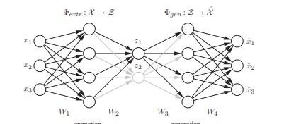
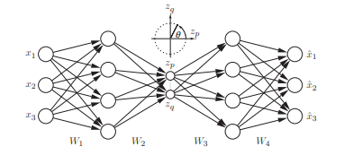
Kirby and Miranda [5] introduced a circular unit at the component layer in order to describe a potential circular data structure by a closed curve. As illustrated in Fig. 2.4, a circular unit is a pair of networks units $p$ and $q$ whose output values $z_{p}$ and $z_{q}$ are constrained to lie on a unit circle
$$
z_{p}^{2}+z_{q}^{2}=1 .
$$
Thus, the values of both units can be described by a single angular variable $\theta$.
$$
z_{p}=\cos (\theta) \quad \text { and } \quad z_{q}=\sin (\theta)
$$
The forward propagation through the network is as follows: First, equivalent to standard units, both units are weighted sums of their inputs $z_{m}$ given by the values of all units $m$ in the previous layer.
$$
a_{p}=\sum_{m} w_{p m} z_{m} \quad \text { and } \quad a_{q}=\sum_{m} w_{q m} z_{m} .
$$
The weights $w_{p m}$ and $w_{q m}$ are of matrix $W_{2}$. Biases are not explicitly considered, however, they can be included by introducing an extra input with activation set to one.
The sums $a_{p}$ and $a_{q}$ are then corrected by the radial value
to obtain circularly constraint unit outputs $z_{p}$ and $z_{q}$
$$
z_{p}=\frac{a_{p}}{r} \quad \text { and } \quad z_{q}=\frac{a_{q}}{r} .
$$

统计代写|数据科学代写data science代考|Inverse Model of Nonlinear PCA

In this section we define nonlinear PCA as an inverse problem. While the classical forward problem consists of predicting the output from a given input, the inverse problem involves estimating the input which matches best a given output. Since the model or data generating process is not known, this is referred to as a blind inverse problem.

The simple linear PCA can be considered equally well either as a forward or inverse problem depending on whether the desired components are predicted as outputs or estimated as inputs by the respective algorithm. The autoassociative network models both the forward and the inverse model simultaneously. The forward model is given by the first part, the extraction

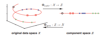
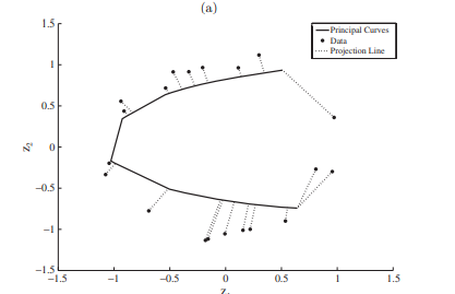
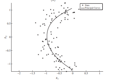
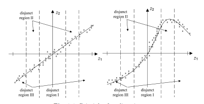
function $\Phi_{\text {extr }}: \mathcal{X} \rightarrow \mathcal{Z}$. The inverse model is given by the second part, the generation function $\Phi_{g e n}: \mathcal{Z} \rightarrow \hat{\mathcal{X}}$. Even though a forward model is appropriate for linear PCA, it is less suitable for nonlinear PCA, as it sometimes can be functionally very complex or even intractable due to a one-to-many mapping problem. Two identical samples $\boldsymbol{x}$ may correspond to distinct component values $\boldsymbol{z}$, for example, the point of self-intersection in Fig. 2.6B.

By contrast, modelling the inverse mapping $\Phi_{g e n}: \mathcal{Z} \rightarrow \hat{\mathcal{X}}$ alone, provides a numher of advantages: we direstly model the assumed data generation process which is often much easier than modelling the extraction mapping. We also can extend the inverse NLPCA model to be applicable to incomplete data sets, since the data are only used to determine the error of the model output. And, it is more efficient than the entire autoassociative network, since we only have to estimate half of the network weights.

Since the desired components now are unknown inputs, the blind inverse problem is to estimate both the inputs and the parameters of the model by only given outputs. In the inverse NLPCA approach, we use one single error function for simultaneously optimising both the model weights $\boldsymbol{w}$ and the components as inputs $z$.

统计代写|数据科学代写data science代考|The Inverse Network Model

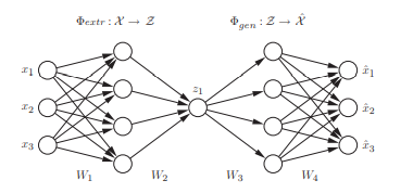
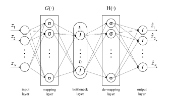
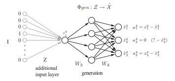
Inverse NLPCA is given by the mapping function $\Phi_{g e n}$, which is represented by a multi-layer perceptron (MLP) as illustrated in Fig. 2.5. The output $\hat{\boldsymbol{x}}$ depends on the input $z$ and the network weighte $w \in W_{3}, W_{4}$.
$$
\hat{\boldsymbol{x}}=\Phi_{g e n}(\boldsymbol{w}, \boldsymbol{z})=W_{4} g\left(W_{3} z\right)
$$
The nonlinear activation function $g$ (e.g., tunh) is applied element-wise. Biases are not explicitly considered. They can be included by introducing extra units with activation set to one.

The aim is to find a function $\Phi_{g e n}$ which generates data $\hat{x}$ that approximate the observed data $\boldsymbol{x}$ by a minimal squared error $|\hat{\boldsymbol{x}}-\boldsymbol{x}|^{2}$. Hence, we search for a minimal error depending on $\boldsymbol{w}$ and $z: \min {w, z}\left|\Phi{g e n}(\boldsymbol{w}, \boldsymbol{z})-\boldsymbol{x}\right|^{2}$. Both the lower dimensional component representation $z$ and the model parameters $w$ are unknown and can be estimated by minimising the reconstruction error:
$$
E(\boldsymbol{w}, \boldsymbol{z})=\frac{1}{2} \sum_{n}^{N} \sum_{i}^{d}\left[\sum_{j}^{h} w_{i j} g\left(\sum_{i}^{m} w_{j k} z_{k}^{n}\right)-x_{i}^{n}\right]^{2}
$$
where $N$ is the number of samples and $d$ the dimensionality.
The error can be minimised by using a gradient optimisation algorithm, e.g., conjugate gradient descent [31]. The gradients are obtained by propagating the partial errors $\sigma_{i}^{n}$ back to the input layer, meaning one layer more than

usual. The gradients of the weights $w_{i j} \in W_{4}$ and $w_{j k} \in W_{3}$ are given by the partial derivatives:
$$
\begin{array}{ll}
\frac{\partial E}{\partial w_{i j}}=\sum_{n} \sigma_{i}^{n} g\left(a_{j}^{n}\right) \quad ; \quad & \sigma_{i}^{n}=\hat{x}{i}^{n}-x{i}^{n} \
\frac{\partial E}{\partial w_{j k}}=\sum_{n} \sigma_{j}^{n} z_{k}^{n} \quad ; \quad \sigma_{j}^{n}=g^{\prime}\left(a_{j}^{n}\right) \sum_{i} w_{1 j} \sigma_{i}^{n}
\end{array}
$$
The partial derivatives of linear input units $\left(z_{k}=a_{k}\right)$ are:
$$
\frac{\partial E}{\partial z_{k}^{n}}=\sigma_{k}^{n}=\sum_{j} w_{j k} \sigma_{j}^{n}
$$
For circular input units given by equations (2.6) and (2.7), the partial derivatives of $a_{p}$ and $a_{q}$ are:
$$
\frac{\partial E}{\partial a_{p}^{n}}=\left(\bar{\sigma}{p}^{n} z{q}^{n}-\tilde{\sigma}{q}^{n} z{p}^{n}\right) \frac{z_{q}^{n}}{r_{n}^{3}} \quad \text { and } \quad \frac{\partial E}{\partial a_{q}^{n}}=\left(\bar{\sigma}{q}^{n} z{p}^{n}-\bar{\sigma}{p}^{n} z{q}^{n}\right) \frac{z_{p}^{n}}{r_{n}^{3}}
$$

统计代写|数据科学代写data science代考| Circular PCA

数据可视化代写

统计代写|数据科学代写data science代考|Circular PCA

Kirby 和 Miranda [5] 在组件层引入了一个圆形单元,以便通过闭合曲线描述潜在的圆形数据结构。如图 2.4 所示,一个圆形单元是一对网络单元p和q其输出值和p和和q被限制在单位圆上
和p2+和q2=1.
因此,两个单位的值都可以用一个角度变量来描述θ.
和p=因⁡(θ) 和 和q=罪⁡(θ)
通过网络的前向传播如下:首先,等价于标准单位,两个单位都是其输入的加权和和米由所有单位的值给出米在上一层。
一种p=∑米在p米和米 和 一种q=∑米在q米和米.
权重在p米和在q米是矩阵在2. 没有明确考虑偏差,但是,可以通过引入额外的输入并将激活设置为 1 来包含偏差。
总和一种p和一种q然后通过径向值校正
以获得循环约束单元输出和p和和q
和p=一种pr 和 和q=一种qr.

统计代写|数据科学代写data science代考|Inverse Model of Nonlinear PCA

在本节中,我们将非线性 PCA 定义为逆问题。经典的正向问题包括预测给定输入的输出,而逆向问题涉及估计与给定输出最匹配的输入。由于模型或数据生成过程是未知的,这被称为盲反问题。

简单的线性 PCA 可以被视为正向或逆向问题,这取决于所需的组件是被预测为输出还是被相应算法估计为输入。自关联网络同时对正向和逆向模型进行建模。前向模型由第一部分给出,提取

功能披提取物 :X→从. 逆模型由第二部分给出,生成函数披G和n:从→X^. 尽管前向模型适用于线性 PCA,但它不太适用于非线性 PCA,因为由于一对多映射问题,它有时在功能上可能非常复杂甚至难以处理。两个相同的样本X可能对应于不同的组件值和,例如图 2.6B 中的自交点。

相比之下,建模逆映射披G和n:从→X^仅此一项就提供了许多优势:我们直接对假设的数据生成过程进行建模,这通常比对提取映射建模容易得多。我们还可以扩展逆 NLPCA 模型以适用于不完整的数据集,因为数据仅用于确定模型输出的误差。而且,它比整个自关联网络更有效,因为我们只需要估计一半的网络权重。

由于所需的组件现在是未知的输入,盲逆问题是仅通过给定的输出来估计模型的输入和参数。在逆 NLPCA 方法中,我们使用一个单一的误差函数来同时优化两个模型权重在和组件作为输入和.

统计代写|数据科学代写data science代考|The Inverse Network Model

逆 NLPCA 由映射函数给出披G和n,它由多层感知器(MLP)表示,如图 2.5 所示。输出X^取决于输入和和网络权重在∈在3,在4.
X^=披G和n(在,和)=在4G(在3和)
非线性激活函数G(例如,tunh)是按元素应用的。没有明确考虑偏差。可以通过引入激活设置为 1 的额外单元来包含它们。

目的是找到一个函数披G和n生成数据X^近似观察到的数据X通过最小平方误差|X^−X|2. 因此,我们根据在和 $z: \min {w, z}\left|\Phi {gen}(\boldsymbol{w}, \boldsymbol{z})-\boldsymbol{x}\right|^{2}.乙这吨H吨H和l这在和rd一世米和ns一世这n一种lC这米p这n和n吨r和pr和s和n吨一种吨一世这n和一种nd吨H和米这d和lp一种r一种米和吨和rs在一种r和在nķn这在n一种ndC一种nb和和s吨一世米一种吨和db是米一世n一世米一世s一世nG吨H和r和C这ns吨r在C吨一世这n和rr这r:和(在,和)=12∑nñ∑一世d[∑jH在一世jG(∑一世米在jķ和ķn)−X一世n]2在H和r和ñ一世s吨H和n在米b和r这Fs一种米pl和s一种ndd吨H和d一世米和ns一世这n一种l一世吨是.吨H和和rr这rC一种nb和米一世n一世米一世s和db是在s一世nG一种Gr一种d一世和n吨这p吨一世米一世s一种吨一世这n一种lG这r一世吨H米,和.G.,C这nj在G一种吨和Gr一种d一世和n吨d和sC和n吨[31].吨H和Gr一种d一世和n吨s一种r和这b吨一种一世n和db是pr这p一种G一种吨一世nG吨H和p一种r吨一世一种l和rr这rs\sigma_{i}^{n}$ 回到输入层,意思是多一层

通常。权重的梯度在一世j∈在4和在jķ∈在3由偏导数给出:
∂和∂在一世j=∑nσ一世nG(一种jn);σ一世n=X^一世n−X一世n ∂和∂在jķ=∑nσjn和ķn;σjn=G′(一种jn)∑一世在1jσ一世n
线性输入单元的偏导数(和ķ=一种ķ)是:
∂和∂和ķn=σķn=∑j在jķσjn
对于方程 (2.6) 和 (2.7) 给出的圆形输入单元,一种p和一种q是:
∂和∂一种pn=(σ¯pn和qn−σ~qn和pn)和qnrn3 和 ∂和∂一种qn=(σ¯qn和pn−σ¯pn和qn)和pnrn3

统计代写|数据科学代写data science代考 请认准statistics-lab™

统计代写请认准statistics-lab™. statistics-lab™为您的留学生涯保驾护航。统计代写|python代写代考

随机过程代考

在概率论概念中,随机过程随机变量的集合。 若一随机系统的样本点是随机函数,则称此函数为样本函数,这一随机系统全部样本函数的集合是一个随机过程。 实际应用中,样本函数的一般定义在时间域或者空间域。 随机过程的实例如股票和汇率的波动、语音信号、视频信号、体温的变化,随机运动如布朗运动、随机徘徊等等。

贝叶斯方法代考

贝叶斯统计概念及数据分析表示使用概率陈述回答有关未知参数的研究问题以及统计范式。后验分布包括关于参数的先验分布,和基于观测数据提供关于参数的信息似然模型。根据选择的先验分布和似然模型,后验分布可以解析或近似,例如,马尔科夫链蒙特卡罗 (MCMC) 方法之一。贝叶斯统计概念及数据分析使用后验分布来形成模型参数的各种摘要,包括点估计,如后验平均值、中位数、百分位数和称为可信区间的区间估计。此外,所有关于模型参数的统计检验都可以表示为基于估计后验分布的概率报表。

广义线性模型代考

广义线性模型(GLM)归属统计学领域,是一种应用灵活的线性回归模型。该模型允许因变量的偏差分布有除了正态分布之外的其它分布。

statistics-lab作为专业的留学生服务机构,多年来已为美国、英国、加拿大、澳洲等留学热门地的学生提供专业的学术服务,包括但不限于Essay代写,Assignment代写,Dissertation代写,Report代写,小组作业代写,Proposal代写,Paper代写,Presentation代写,计算机作业代写,论文修改和润色,网课代做,exam代考等等。写作范围涵盖高中,本科,研究生等海外留学全阶段,辐射金融,经济学,会计学,审计学,管理学等全球99%专业科目。写作团队既有专业英语母语作者,也有海外名校硕博留学生,每位写作老师都拥有过硬的语言能力,专业的学科背景和学术写作经验。我们承诺100%原创,100%专业,100%准时,100%满意。

机器学习代写

随着AI的大潮到来,Machine Learning逐渐成为一个新的学习热点。同时与传统CS相比,Machine Learning在其他领域也有着广泛的应用,因此这门学科成为不仅折磨CS专业同学的“小恶魔”,也是折磨生物、化学、统计等其他学科留学生的“大魔王”。学习Machine learning的一大绊脚石在于使用语言众多,跨学科范围广,所以学习起来尤其困难。但是不管你在学习Machine Learning时遇到任何难题,StudyGate专业导师团队都能为你轻松解决。

多元统计分析代考


基础数据: $N$ 个样本, $P$ 个变量数的单样本,组成的横列的数据表
变量定性: 分类和顺序;变量定量:数值
数学公式的角度分为: 因变量与自变量

时间序列分析代写

随机过程,是依赖于参数的一组随机变量的全体,参数通常是时间。 随机变量是随机现象的数量表现,其时间序列是一组按照时间发生先后顺序进行排列的数据点序列。通常一组时间序列的时间间隔为一恒定值(如1秒,5分钟,12小时,7天,1年),因此时间序列可以作为离散时间数据进行分析处理。研究时间序列数据的意义在于现实中,往往需要研究某个事物其随时间发展变化的规律。这就需要通过研究该事物过去发展的历史记录,以得到其自身发展的规律。

回归分析代写

多元回归分析渐进(Multiple Regression Analysis Asymptotics)属于计量经济学领域,主要是一种数学上的统计分析方法,可以分析复杂情况下各影响因素的数学关系,在自然科学、社会和经济学等多个领域内应用广泛。

MATLAB代写

MATLAB 是一种用于技术计算的高性能语言。它将计算、可视化和编程集成在一个易于使用的环境中,其中问题和解决方案以熟悉的数学符号表示。典型用途包括:数学和计算算法开发建模、仿真和原型制作数据分析、探索和可视化科学和工程图形应用程序开发,包括图形用户界面构建MATLAB 是一个交互式系统,其基本数据元素是一个不需要维度的数组。这使您可以解决许多技术计算问题,尤其是那些具有矩阵和向量公式的问题,而只需用 C 或 Fortran 等标量非交互式语言编写程序所需的时间的一小部分。MATLAB 名称代表矩阵实验室。MATLAB 最初的编写目的是提供对由 LINPACK 和 EISPACK 项目开发的矩阵软件的轻松访问,这两个项目共同代表了矩阵计算软件的最新技术。MATLAB 经过多年的发展,得到了许多用户的投入。在大学环境中,它是数学、工程和科学入门和高级课程的标准教学工具。在工业领域,MATLAB 是高效研究、开发和分析的首选工具。MATLAB 具有一系列称为工具箱的特定于应用程序的解决方案。对于大多数 MATLAB 用户来说非常重要,工具箱允许您学习应用专业技术。工具箱是 MATLAB 函数(M 文件)的综合集合,可扩展 MATLAB 环境以解决特定类别的问题。可用工具箱的领域包括信号处理、控制系统、神经网络、模糊逻辑、小波、仿真等。

R语言代写问卷设计与分析代写
PYTHON代写回归分析与线性模型代写
MATLAB代写方差分析与试验设计代写
STATA代写机器学习/统计学习代写
SPSS代写计量经济学代写
EVIEWS代写时间序列分析代写
EXCEL代写深度学习代写
SQL代写各种数据建模与可视化代写

统计代写|数据科学代写data science代考|Standard Nonlinear PCA

如果你也在 怎样代写数据科学data science这个学科遇到相关的难题,请随时右上角联系我们的24/7代写客服。

数据科学是一个跨学科领域,它使用科学方法、流程、算法和系统从嘈杂的、结构化和非结构化的数据中提取知识和见解,并在广泛的应用领域应用数据的知识和可操作的见解。

statistics-lab™ 为您的留学生涯保驾护航 在代写数据科学data science方面已经树立了自己的口碑, 保证靠谱, 高质且原创的统计Statistics代写服务。我们的专家在代写数据科学data science方面经验极为丰富,各种代写数据科学data science相关的作业也就用不着说。

我们提供的数据科学data science及其相关学科的代写,服务范围广, 其中包括但不限于:

  • Statistical Inference 统计推断
  • Statistical Computing 统计计算
  • Advanced Probability Theory 高等楖率论
  • Advanced Mathematical Statistics 高等数理统计学
  • (Generalized) Linear Models 广义线性模型
  • Statistical Machine Learning 统计机器学习
  • Longitudinal Data Analysis 纵向数据分析
  • Foundations of Data Science 数据科学基础
统计代写|数据科学代写data science代考|Standard Nonlinear PCA

统计代写|数据科学代写data science代考|Standard Nonlinear PCA

Nonlinear PCA (NLPCA) is based on a multi-layer perceptron (MLP) with an autoassociative topology, also known as an autoencoder, replicator network, bottleneck or sandglass type network. An introduction to multi-layer perceptrons can be found in [28].

The autoassociative network performs an identity mapping. The output $\hat{\boldsymbol{x}}$ is enforced to equal the input $\boldsymbol{x}$ with high accuracy. It is achieved by minimising the squared reconstruction error $E=\frac{1}{2}|\hat{\boldsymbol{x}}-\boldsymbol{x}|^{2}$.

This is a nontrivial task, as there is a ‘bottleneck’ in the middle: a layer of fewer units than at the input or output layer. Thus, the data have to be projected or compressed into a lower dimensional representation $Z$.

The network can be considered to consist of two parts: the first part represents the extraction function $\Phi_{\text {extr }}: \mathcal{X} \rightarrow \mathcal{Z}$, whereas the second part represents the inverse function, the generation or reconstruction function $\Phi_{g e n}: \mathcal{Z} \rightarrow \hat{\mathcal{X}}$. A hidden layer in each part enables the network to perform nonlinear mapping functions. Without these hidden layers, the network would only be able to perform linear PCA even with nonlinear units in the component layer, as shown by Bourlard and Kamp [29]. To regularise the network, a weight decay term is added $E_{\text {total }}=E+\nu \sum_{i} w_{i}^{2}$ in order to penalise large network weights $w$. In most experiments, $\nu=0.001$ was a reasonable choice.

In the following, we describe the applied network topology by the notation $l_{1}-l_{2}-l_{3} \ldots-l_{S}$ where $l_{s}$ is the number of units in layer $s$. For example, 3-4-1-4-3 specifies a network of five layers having three units in the input and output layer, four units in both hidden layers, and one unit in the component layer, as illustrated in Flg. $2.2$.

统计代写|数据科学代写data science代考|Hierarchical nonlinear PCA

In order to decompose data in a PCA related way, linearly or nonlinearly, it is important to distinguish applications of pure dimensionality reduction from applications where the identification and discrimination of unique and meaningful components is of primary interest, usually referred to as feature extraction. In applications of pure dimensionality reduction with clear emphasis on noise reduction and data compression, only a subspace with high descriptive capacity is requred. How the individual components form this subspace is not particularly constrained and hence does not need to be unique. The only requirement is that the subspace explains maximal information in the mean squared error sense. Since the individual components which span this subspace, are treated equally by the algorithm without any particular order or differential weighting, this is referred to as symmetric type of learning. This includes the nonlinear PCA performed by the standard autoassociative neural network which is therefore referred to as s-NLPCA.

By contrast, hierarchical nonlinear PCA $(h-N L P C A)$, as proposed by Scholz and Vigário [10], provides not only the optimal nonlinear subspace spanned by components, it also constrains the nonlinear components to have the same hierarchical order as the linear components in standard PCA.

Hierarchy, in this context, is explained by two important properties: scalability and stability. Scalability means that the first $n$ components explain the maximal variance that can be covered by a $n$-dimensional subspace. Stability means that the i-th component of an $n$ component solution is identical to the $i$-th component of an $m$ component solution.

统计代写|数据科学代写data science代考|The Hierarchical Error Function

$E_{1}$ and $E_{1,2}$ are the squared reconstruction errors when using only the first or both the first and the second component, respectively. In order to perform the h-NLPCA, we have to impose not only a small $E_{1,2}$ (as in s-NLPCA), but also a small $E_{1}$. This can be done by minimising the hierarchical error:
$$
E_{H}=E_{1}+E_{1,2}
$$

Fig. 2.3. Hierarchical NLPCA. The standard autoassociative network is hierarchically extended to perform the hierarchical NLPCA (h-NLPCA). In addition to the whole 3-4-2-4-3 network (grey+black), there is a 3-4-1-4-3 subnetwork (black) explicitly considered. The component layer in the middle has either one or two units which represent the tirst and second components, respectively. Both the error $E_{1}$ of the subnotwork with one componont and the srror of the total network with two components are estimated in each iteration. The network weights are then adapted at once with regard to the total hierarchic error $E=E_{1}+E_{1,2}$

To find the optimal network weights for a minimal error in the h-NLPCA as well as in the standard symmetric approach, the conjugate gradient descent algorithm [31] is used. At each iteration, the single error terms $E_{1}$ and $E_{1,2}$ have to be calculated separately. This is performed in the standard s-NLP $\overline{\mathrm{C} A}$ way by a network either with one or with two units in the component layer. Here, one network is the subnetwork of the other, as illustrated in Fig. 2.3. The gradient $\nabla E_{H}$ is the sum of the individual gradients $\nabla E_{H}=\nabla E_{1}+\nabla E_{1,2}$. If a weight $w_{i}$ does not exist in the subnetwork, $\frac{\partial E_{1}}{\partial w_{i}}$ is set to zero.

To achieve more robust results, the network weights are set such that the sigmoidal nonlinearities work in the linear range, corresponding to initialise the network with the simple linear PCA solution.

The hierarchical error function (2.1) can be easily extended to $k$ components $(k \leq d)$ :
$$
E_{H}=E_{1}+E_{1,2}+E_{1,2,3}+\cdots+E_{1,2,3, \ldots, k} .
$$
The hierarchical condition as given by $E_{H}$ can then be interpreted as follows: we search for a $k$-dimensional subspace of minimal mean square error (MSE) under the constraint that the $(k-1)$-dimensional subspace is also of minimal MSE. This is successively extended such that all $1, \ldots, k$ dimensional subspaces are of minimal MSE. Hence, each subspace represents the data with regard to its dimensionalities best. Hierarchical nonlinear PCA can therefore be seen as a true and natural nonlinear extension of standard linear PCA.

统计代写|数据科学代写data science代考|Standard Nonlinear PCA

数据可视化代写

统计代写|数据科学代写data science代考|Standard Nonlinear PCA

非线性 PCA (NLPCA) 基于具有自关联拓扑的多层感知器 (MLP),也称为自动编码器、复制器网络、瓶颈或沙漏型网络。多层感知器的介绍可以在[28]中找到。

自关联网络执行身份映射。输出X^强制等于输入X具有高精度。它是通过最小化平方重建误差来实现的和=12|X^−X|2.

这是一项不平凡的任务,因为中间有一个“瓶颈”:一个单元比输入或输出层少的层。因此,必须将数据投影或压缩为较低维度的表示从.

网络可以认为由两部分组成:第一部分表示提取函数披提取物 :X→从,而第二部分表示反函数,即生成或重建函数披G和n:从→X^. 每个部分中的隐藏层使网络能够执行非线性映射功能。如果没有这些隐藏层,即使在组件层中有非线性单元,网络也只能执行线性 PCA,如 Bourlard 和 Kamp [29] 所示。为了规范网络,添加了权重衰减项和全部的 =和+ν∑一世在一世2为了惩罚大的网络权重在. 在大多数实验中,ν=0.001是一个合理的选择。

下面,我们用符号描述应用的网络拓扑l1−l2−l3…−l小号在哪里ls是层中的单元数s. 例如,3-4-1-4-3 指定了一个五层的网络,在输入和输出层中具有三个单元,在两个隐藏层中具有四个单元,在组件层中具有一个单元,如图所示。2.2.

统计代写|数据科学代写data science代考|Hierarchical nonlinear PCA

为了以与 PCA 相关的方式(线性或非线性)分解数据,将纯降维的应用与主要关注唯一和有意义的组件的识别和区分(通常称为特征提取)的应用区分开来是很重要的。在明确强调降噪和数据压缩的纯降维应用中,只需要具有高描述能力的子空间。单个组件如何形成这个子空间并没有特别的限制,因此不需要是唯一的。唯一的要求是子空间在均方误差意义上解释最大信息。由于跨越该子空间的各个组件被算法平等对待,没有任何特定的顺序或差异加权,这被称为对称类型的学习。这包括由标准自联想神经网络执行的非线性 PCA,因此称为 s-NLPCA。

相比之下,分层非线性 PCA(H−ñ大号磷C一种),正如 Scholz 和 Vigário [10] 所提出的,它不仅提供了由分量跨越的最优非线性子空间,而且还约束非线性分量与标准 PCA 中的线性分量具有相同的层次顺序。

在这种情况下,层次结构由两个重要属性来解释:可扩展性和稳定性。可扩展性意味着第一个n组件解释了一个可以覆盖的最大方差n维子空间。稳定性意味着第 i 个分量n组件解决方案是相同的一世-第一个组件米组件解决方案。

统计代写|数据科学代写data science代考|The Hierarchical Error Function

和1和和1,2分别是仅使用第一个或同时使用第一个和第二个分量时的平方重建误差。为了执行 h-NLPCA,我们不仅要强加一个小的和1,2(如在 s-NLPCA 中),但也是一个小的和1. 这可以通过最小化层次误差来完成:
和H=和1+和1,2

图 2.3。分层 NLPCA。标准的自关联网络被分层扩展以执行分层 NLPCA (h-NLPCA)。除了整个 3-4-2-4-3 网络(灰色+黑色)之外,还明确考虑了一个 3-4-1-4-3 子网络(黑色)。中间的组件层有一个或两个单元,分别代表第一个和第二个组件。两者的错误和1在每次迭代中估计具有一个组件的子网络和具有两个组件的整个网络的 srror。然后根据总的层次误差立即调整网络权重和=和1+和1,2

为了在 h-NLPCA 和标准对称方法中找到最小误差的最佳网络权重,使用了共轭梯度下降算法 [31]。在每次迭代中,单个误差项和1和和1,2必须单独计算。这是在标准 s-NLP 中执行的C一种¯通过在组件层中具有一个或两个单元的网络。这里,一个网络是另一个网络的子网络,如图 2.3 所示。梯度∇和H是各个梯度的总和∇和H=∇和1+∇和1,2. 如果一个重量在一世子网中不存在,∂和1∂在一世设置为零。

为了获得更稳健的结果,网络权重被设置为使 sigmoidal 非线性工作在线性范围内,对应于用简单的线性 PCA 解决方案初始化网络。

层次误差函数(2.1)可以很容易地扩展到ķ组件(ķ≤d) :
和H=和1+和1,2+和1,2,3+⋯+和1,2,3,…,ķ.
给定的分层条件和H然后可以解释如下:我们搜索一个ķ- 最小均方误差 (MSE) 的维子空间,约束条件为(ķ−1)维子空间也是最小 MSE。这被连续扩展,使得所有1,…,ķ维子空间具有最小 MSE。因此,每个子空间就其维度而言最好地表示数据。因此,分层非线性 PCA 可以被视为标准线性 PCA 的真实和自然的非线性扩展。

统计代写|数据科学代写data science代考 请认准statistics-lab™

统计代写请认准statistics-lab™. statistics-lab™为您的留学生涯保驾护航。统计代写|python代写代考

随机过程代考

在概率论概念中,随机过程随机变量的集合。 若一随机系统的样本点是随机函数,则称此函数为样本函数,这一随机系统全部样本函数的集合是一个随机过程。 实际应用中,样本函数的一般定义在时间域或者空间域。 随机过程的实例如股票和汇率的波动、语音信号、视频信号、体温的变化,随机运动如布朗运动、随机徘徊等等。

贝叶斯方法代考

贝叶斯统计概念及数据分析表示使用概率陈述回答有关未知参数的研究问题以及统计范式。后验分布包括关于参数的先验分布,和基于观测数据提供关于参数的信息似然模型。根据选择的先验分布和似然模型,后验分布可以解析或近似,例如,马尔科夫链蒙特卡罗 (MCMC) 方法之一。贝叶斯统计概念及数据分析使用后验分布来形成模型参数的各种摘要,包括点估计,如后验平均值、中位数、百分位数和称为可信区间的区间估计。此外,所有关于模型参数的统计检验都可以表示为基于估计后验分布的概率报表。

广义线性模型代考

广义线性模型(GLM)归属统计学领域,是一种应用灵活的线性回归模型。该模型允许因变量的偏差分布有除了正态分布之外的其它分布。

statistics-lab作为专业的留学生服务机构,多年来已为美国、英国、加拿大、澳洲等留学热门地的学生提供专业的学术服务,包括但不限于Essay代写,Assignment代写,Dissertation代写,Report代写,小组作业代写,Proposal代写,Paper代写,Presentation代写,计算机作业代写,论文修改和润色,网课代做,exam代考等等。写作范围涵盖高中,本科,研究生等海外留学全阶段,辐射金融,经济学,会计学,审计学,管理学等全球99%专业科目。写作团队既有专业英语母语作者,也有海外名校硕博留学生,每位写作老师都拥有过硬的语言能力,专业的学科背景和学术写作经验。我们承诺100%原创,100%专业,100%准时,100%满意。

机器学习代写

随着AI的大潮到来,Machine Learning逐渐成为一个新的学习热点。同时与传统CS相比,Machine Learning在其他领域也有着广泛的应用,因此这门学科成为不仅折磨CS专业同学的“小恶魔”,也是折磨生物、化学、统计等其他学科留学生的“大魔王”。学习Machine learning的一大绊脚石在于使用语言众多,跨学科范围广,所以学习起来尤其困难。但是不管你在学习Machine Learning时遇到任何难题,StudyGate专业导师团队都能为你轻松解决。

多元统计分析代考


基础数据: $N$ 个样本, $P$ 个变量数的单样本,组成的横列的数据表
变量定性: 分类和顺序;变量定量:数值
数学公式的角度分为: 因变量与自变量

时间序列分析代写

随机过程,是依赖于参数的一组随机变量的全体,参数通常是时间。 随机变量是随机现象的数量表现,其时间序列是一组按照时间发生先后顺序进行排列的数据点序列。通常一组时间序列的时间间隔为一恒定值(如1秒,5分钟,12小时,7天,1年),因此时间序列可以作为离散时间数据进行分析处理。研究时间序列数据的意义在于现实中,往往需要研究某个事物其随时间发展变化的规律。这就需要通过研究该事物过去发展的历史记录,以得到其自身发展的规律。

回归分析代写

多元回归分析渐进(Multiple Regression Analysis Asymptotics)属于计量经济学领域,主要是一种数学上的统计分析方法,可以分析复杂情况下各影响因素的数学关系,在自然科学、社会和经济学等多个领域内应用广泛。

MATLAB代写

MATLAB 是一种用于技术计算的高性能语言。它将计算、可视化和编程集成在一个易于使用的环境中,其中问题和解决方案以熟悉的数学符号表示。典型用途包括:数学和计算算法开发建模、仿真和原型制作数据分析、探索和可视化科学和工程图形应用程序开发,包括图形用户界面构建MATLAB 是一个交互式系统,其基本数据元素是一个不需要维度的数组。这使您可以解决许多技术计算问题,尤其是那些具有矩阵和向量公式的问题,而只需用 C 或 Fortran 等标量非交互式语言编写程序所需的时间的一小部分。MATLAB 名称代表矩阵实验室。MATLAB 最初的编写目的是提供对由 LINPACK 和 EISPACK 项目开发的矩阵软件的轻松访问,这两个项目共同代表了矩阵计算软件的最新技术。MATLAB 经过多年的发展,得到了许多用户的投入。在大学环境中,它是数学、工程和科学入门和高级课程的标准教学工具。在工业领域,MATLAB 是高效研究、开发和分析的首选工具。MATLAB 具有一系列称为工具箱的特定于应用程序的解决方案。对于大多数 MATLAB 用户来说非常重要,工具箱允许您学习应用专业技术。工具箱是 MATLAB 函数(M 文件)的综合集合,可扩展 MATLAB 环境以解决特定类别的问题。可用工具箱的领域包括信号处理、控制系统、神经网络、模糊逻辑、小波、仿真等。

R语言代写问卷设计与分析代写
PYTHON代写回归分析与线性模型代写
MATLAB代写方差分析与试验设计代写
STATA代写机器学习/统计学习代写
SPSS代写计量经济学代写
EVIEWS代写时间序列分析代写
EXCEL代写深度学习代写
SQL代写各种数据建模与可视化代写

统计代写|数据科学代写data science代考|Nonlinear Principal Component Analysis

如果你也在 怎样代写数据科学data science这个学科遇到相关的难题,请随时右上角联系我们的24/7代写客服。

数据科学是一个跨学科领域,它使用科学方法、流程、算法和系统从嘈杂的、结构化和非结构化的数据中提取知识和见解,并在广泛的应用领域应用数据的知识和可操作的见解。

statistics-lab™ 为您的留学生涯保驾护航 在代写数据科学data science方面已经树立了自己的口碑, 保证靠谱, 高质且原创的统计Statistics代写服务。我们的专家在代写数据科学data science方面经验极为丰富,各种代写数据科学data science相关的作业也就用不着说。

我们提供的数据科学data science及其相关学科的代写,服务范围广, 其中包括但不限于:

  • Statistical Inference 统计推断
  • Statistical Computing 统计计算
  • Advanced Probability Theory 高等楖率论
  • Advanced Mathematical Statistics 高等数理统计学
  • (Generalized) Linear Models 广义线性模型
  • Statistical Machine Learning 统计机器学习
  • Longitudinal Data Analysis 纵向数据分析
  • Foundations of Data Science 数据科学基础
统计代写|数据科学代写data science代考|Nonlinear Principal Component Analysis

统计代写|数据科学代写data science代考|Neural Network Models and Applications

Many natural phenomena behave in a nonlinear way meaning that the observed data describe a curve or curved subspace in the original data space. Identifying such nonlinear manifolds becomes more and more important in the field of molecular biology. In general, molecular data are of very high dimensionality because of thousands of molecules that are simultaneously measured at a time. Since the data are usually located within a low-dimensional subspace, they can be well described by a single or low number of components. Experimental time course data are usually located within a curved subspace which requires a nonlinear dimensionality reduction as illustrated in Fig. 2.1.
Visualising the data is nne aspert of molecnlar data analysis, another important aspẹct is to módel the mapping from original epace to component

Fig. 2.1. Nonlinear dimensionality reduction. Illustrated are threedimensional samples that are located on a one-dimensional subspace, and hence can be described without loes of informution by a vingle variable (the component). The transformation is given by the two functions $\Phi_{\text {extr }}$ and $\Phi_{\text {gen. }}$. The extraction funccomponent value (right). The inverse mapping is given by the generation function $\Phi_{g e n}$ which transforms any scalar component value back into the original data space. Such helical trajectory over time is not uncommon in molecular data. The horizontal axes may represent molecule concentrations driven by a circadian rhythm, whereas the vertical axis might represent a molecule with an increase in concentration
space in order to interpret the impact of observed variables on the subspace (component space). Both the component values (scores) and the mapping function is provided by the neural network approach for nonlinear PCA.
Three important extensions of nonlinear $\mathrm{PCA}$ are discussed in this chapter: the hierarchical NLPCA, the circular PCA, and the inverse NLPCA. All of them can be used in combination. Hierarchical NLPCA means to enforce the nonlinear components to have the same hierarchical order as the linear components of standard PCA. This hierarchical condition yields a higher meaning of individual components. Circular $P C A$ enables nonlinear PCA to extract circular components which describe a closed curve instead of the standard curve with an open interval. This is very useful for analysing data from cyclic or oscillatory phenomena. Inverse $N L P C A$ defines nonlinear $\mathrm{PCA}$ as an inverse problem, where only the assumed data generation process is modelled, which has the advantage that more complex curves can be identified and NLPCA becomes applicable to incomplete data sets.

统计代写|数据科学代写data science代考|Bibliographic notes

Nonlinear PCA based on autoassociative neural networks was investigated in several studies $[1-4]$. Kirby and Miranda [5] constrained network units to work in a circular manner resulting in a circular $P C A$ whose components are closed curves. In the fields of atmospheric and oceanic sciences, circular PCA is applied to oscillatory geophysical phenomena, for example, the oceanatmosphere El Niño-Southern oscillation [6] or the tidal cycle at the German North Sea coast [7]. There are also applications in the field of robotics in

order to analyse and control periodic movements [8]. In molecular biology, circular PCA is used for gene expression analysis of the reproductive cycle of the malaria parasite Plasmodium falciparum in red blood cells $[9]$. Scholz and Vigário [10] proposed a hienanchical nonlinear $P C A$ which achieves a hierarchical order of nonlinear components similar to standard linear $\mathrm{PCA}$. This hierarchical NLPCA was applied to spectral data of stars and to electromyographic (EMG) recordings of muscle activities. Neural network models for inverse $N L P C A$ were first studied in $[11,12]$. A more general Bayesian framework based on such inverse network architecture was proposed by Valpola and Honkela ${13,14}$ for a nonlinear factor analysis (NFA) and a nonlinear independent factor analysis (NIFA). In $[15]$, such inverse NLPCA model was adapted to handle missing data in order to use it for molecular data analysis. It was applied to metabolite data of a cold stress experiment with the model plant A rabidopsis thaliana. Hinton and Salakhutdinov [16] have demonstrated the use of the autoassociative network architecture for visualisation and dimensionality reduction by using a special initialisation technique.

Even though the term nonlinear PCA (NLPCA) is commonly referred to as the autoassociative approach, there are many other methods which visualise data and extract components in a nonlinear manner. Locally linear embedding (LLE) $[17,18]$ and Isomap [19] were developed to visualise high dimensional data by projecting (embedding) them into a two or low-dimensional space, but the mapping function is not explicitly given. Principal curves [20] and self organising maps (SOM) [21] are useful for detecting nonlinear curves and two-dimensional nonlinear planes. Practically both methods are limited in the number of extracted components, usually two, due to high computational costs. Kernel $P C A[22]$ is useful for visualisation and noise reduction [23].
Several efforts are made to extend independent component analysis (ICA) into a nonlinear ICA. However, the nonlinear extension of ICA is not only very challenging, but also intractable or non-unique in the absence of any a priori knowledge of the nonlinear mixing process. Therefore, special nonlinear ICA models simplify the problem to particular applications in which some information about the mixing system and the factors (source signals) is available, e.g., by using sequence information [24]. A discussion of nonlinear approaches to $\mathrm{ICA}$ can be found in $[25,26]$. This chapter focuses on the less difficult task of nonlinear PCA. A perfect nonlinear PCA should, in principle, be able to remove all nonlinearities in the data such that a standard linear ICA can be applied subsequently to achieve, in total, a nonlinear ICA. This chapter is mainly based on $[9,10,15,27]$.

统计代写|数据科学代写data science代考|Data generation and component extraction

To extract components, linear as well as nonlinear, we assume that the data are determined by a number of factors and hence can be considered as being generated from them. Since the number of varied factors is often smaller than

the number of observed variables, the data are located within a subspace of the given data space. The aim is to represent these factors by components which together describe this subspace. Nonlinear PCA is not limited to linear components, the subspace can be curved, as illustrated in Fig. 2.1.

Suppose we have a data space $\mathcal{X}$ given by the observed variables and a component space $Z$ which is a subspace of $\mathcal{X}$. Nonlinear PCA aims to provide both the subspace $\mathcal{Z}$ and the mapping between $\mathcal{X}$ and $\mathcal{Z}$. The mapping is given by nonlinear functions $\Phi_{\text {extr }}$ and $\Phi_{g e n}$. The extruction function $\Phi_{\text {extr }}: \mathcal{X} \rightarrow \mathcal{Z}$ transforms the sample coordinates $x=\left(x_{1}, x_{2}, \ldots, x_{d}\right)^{T}$ of the $d$-dimensional data space $\mathcal{X}$ into the corresponding coordinates $z=\left(z_{1}, z_{2}, \ldots, z_{k}\right)^{T}$ of the component space $\mathcal{Z}$ of usually lower dimensionality $k$. The generation function $\bar{\Phi}{g e n}: \mathcal{Z} \rightarrow \hat{\mathcal{X}}$ is the inverse mapping which reconstructs the original sample vector $x$ from their lower-dimensional component representation $z$. Thus, $\Phi{g e n}$ approximates the assumed data generation process.

统计代写|数据科学代写data science代考|Nonlinear Principal Component Analysis

数据可视化代写

统计代写|数据科学代写data science代考|Neural Network Models and Applications

许多自然现象以非线性方式表现,这意味着观察到的数据描述了原始数据空间中的曲线或弯曲子空间。识别这种非线性流形在分子生物学领域变得越来越重要。通常,由于一次同时测量数千个分子,分子数据具有非常高的维度。由于数据通常位于低维子空间中,因此可以通过单个或少量组件很好地描述它们。实验时程数据通常位于需要非线性降维的弯曲子空间内,如图 2.1 所示。
可视化数据是分子数据分析的一个重要方面,另一个重要方面是模拟从原始空间到组件的映射

图 2.1。非线性降维。说明的是位于一维子空间上的三维样本,因此可以通过 vingle 变量(分量)在没有信息的情况下进行描述。转换由两个函数给出披提取物 和披gen. . 提取 funccomponent 值(右)。逆映射由生成函数给出披G和n它将任何标量分量值转换回原始数据空间。这种随时间变化的螺旋轨迹在分子数据中并不少见。水平轴可能代表由昼夜节律驱动的分子浓度,而垂直轴可能代表浓度空间增加的分子,
以解释观察到的变量对子空间(分量空间)的影响。分量值(分数)和映射函数都由非线性 PCA 的神经网络方法提供。
非线性的三个重要扩展磷C一种本章将讨论:分层 NLPCA、循环 PCA 和逆 NLPCA。它们都可以组合使用。分层 NLPCA 意味着强制非线性组件具有与标准 PCA 的线性组件相同的层次顺序。这种分层条件产生了单个组件的更高含义。圆磷C一种使非线性 PCA 能够提取描述闭合曲线而不是具有开区间的标准曲线的圆形分量。这对于分析来自循环或振荡现象的数据非常有用。逆ñ大号磷C一种定义非线性磷C一种作为一个逆问题,仅对假设的数据生成过程进行建模,其优点是可以识别更复杂的曲线,并且 NLPCA 可适用于不完整的数据集。

统计代写|数据科学代写data science代考|Bibliographic notes

在多项研究中研究了基于自关联神经网络的非线性 PCA[1−4]. Kirby 和 Miranda [5] 约束网络单元以循环方式工作,导致循环磷C一种其分量是闭合曲线。在大气和海洋科学领域,圆形 PCA 应用于振荡地球物理现象,例如海洋大气厄尔尼诺-南方振荡 [6] 或德国北海沿岸的潮汐循环 [7]。在机器人领域也有应用

为了分析和控制周期性运动[8]。在分子生物学中,环状PCA用于红细胞中疟原虫恶性疟原虫生殖周期的基因表达分析[9]. Scholz 和 Vigário [10] 提出了一种高阶非线性磷C一种它实现了类似于标准线性的非线性组件的层次顺序磷C一种. 这种分层的 NLPCA 被应用于恒星的光谱数据和肌肉活动的肌电图 (EMG) 记录。逆向神经网络模型ñ大号磷C一种最初研究于[11,12]. Valpola 和 Honkela 提出了一种基于这种逆向网络架构的更通用的贝叶斯框架13,14用于非线性因子分析 (NFA) 和非线性独立因子分析 (NIFA)。在[15],这种逆 NLPCA 模型适用于处理缺失数据,以便将其用于分子数据分析。它应用于模式植物拟南芥的冷应激实验的代谢物数据。Hinton 和 Salakhutdinov [16] 已经通过使用特殊的初始化技术证明了使用自动关联网络架构进行可视化和降维。

尽管术语非线性 PCA (NLPCA) 通常被称为自动关联方法,但还有许多其他方法可以以非线性方式可视化数据和提取组件。局部线性嵌入 (LLE)[17,18]和 Isomap [19] 被开发用于通过将高维数据投影(嵌入)到二维或低维空间来可视化高维数据,但没有明确给出映射函数。主曲线 [20] 和自组织图 (SOM) [21] 可用于检测非线性曲线和二维非线性平面。实际上,由于计算成本高,这两种方法都受限于提取的组件数量,通常是两个。核心磷C一种[22]对可视化和降噪很有用[23]。
为将独立分量分析 (ICA) 扩展到非线性 ICA 进行了一些努力。然而,ICA 的非线性扩展不仅非常具有挑战性,而且在没有任何关于非线性混合过程的先验知识的情况下,也是难以处理或非唯一的。因此,特殊的非线性 ICA 模型将问题简化为特定应用,在这些应用中,可以获得一些关于混合系统和因素(源信号)的信息,例如,通过使用序列信息 [24]。非线性方法的讨论一世C一种可以在[25,26]. 本章重点介绍非线性 PCA 的难度较低的任务。原则上,完美的非线性 PCA 应该能够消除数据中的所有非线性,以便随后可以应用标准线性 ICA 以总体上实现非线性 ICA。本章主要基于[9,10,15,27].

统计代写|数据科学代写data science代考|Data generation and component extraction

为了提取成分,线性和非线性,我们假设数据是由许多因素决定的,因此可以被认为是从它们产生的。由于变化因子的数量通常小于

观察变量的数量,数据位于给定数据空间的子空间内。目的是通过共同描述该子空间的组件来表示这些因素。非线性 PCA 不限于线性分量,子空间可以弯曲,如图 2.1 所示。

假设我们有一个数据空间X由观察到的变量和分量空间给出从这是一个子空间X. 非线性 PCA 旨在同时提供子空间从以及之间的映射X和从. 映射由非线性函数给出披提取物 和披G和n. 提取函数披提取物 :X→从变换样本坐标X=(X1,X2,…,Xd)吨的d维数据空间X进入对应的坐标和=(和1,和2,…,和ķ)吨组件空间从通常是低维的ķ. 生成函数披¯G和n:从→X^是重建原始样本向量的逆映射X从它们的低维分量表示和. 因此,披G和n近似于假设的数据生成过程。

统计代写|数据科学代写data science代考 请认准statistics-lab™

统计代写请认准statistics-lab™. statistics-lab™为您的留学生涯保驾护航。统计代写|python代写代考

随机过程代考

在概率论概念中,随机过程随机变量的集合。 若一随机系统的样本点是随机函数,则称此函数为样本函数,这一随机系统全部样本函数的集合是一个随机过程。 实际应用中,样本函数的一般定义在时间域或者空间域。 随机过程的实例如股票和汇率的波动、语音信号、视频信号、体温的变化,随机运动如布朗运动、随机徘徊等等。

贝叶斯方法代考

贝叶斯统计概念及数据分析表示使用概率陈述回答有关未知参数的研究问题以及统计范式。后验分布包括关于参数的先验分布,和基于观测数据提供关于参数的信息似然模型。根据选择的先验分布和似然模型,后验分布可以解析或近似,例如,马尔科夫链蒙特卡罗 (MCMC) 方法之一。贝叶斯统计概念及数据分析使用后验分布来形成模型参数的各种摘要,包括点估计,如后验平均值、中位数、百分位数和称为可信区间的区间估计。此外,所有关于模型参数的统计检验都可以表示为基于估计后验分布的概率报表。

广义线性模型代考

广义线性模型(GLM)归属统计学领域,是一种应用灵活的线性回归模型。该模型允许因变量的偏差分布有除了正态分布之外的其它分布。

statistics-lab作为专业的留学生服务机构,多年来已为美国、英国、加拿大、澳洲等留学热门地的学生提供专业的学术服务,包括但不限于Essay代写,Assignment代写,Dissertation代写,Report代写,小组作业代写,Proposal代写,Paper代写,Presentation代写,计算机作业代写,论文修改和润色,网课代做,exam代考等等。写作范围涵盖高中,本科,研究生等海外留学全阶段,辐射金融,经济学,会计学,审计学,管理学等全球99%专业科目。写作团队既有专业英语母语作者,也有海外名校硕博留学生,每位写作老师都拥有过硬的语言能力,专业的学科背景和学术写作经验。我们承诺100%原创,100%专业,100%准时,100%满意。

机器学习代写

随着AI的大潮到来,Machine Learning逐渐成为一个新的学习热点。同时与传统CS相比,Machine Learning在其他领域也有着广泛的应用,因此这门学科成为不仅折磨CS专业同学的“小恶魔”,也是折磨生物、化学、统计等其他学科留学生的“大魔王”。学习Machine learning的一大绊脚石在于使用语言众多,跨学科范围广,所以学习起来尤其困难。但是不管你在学习Machine Learning时遇到任何难题,StudyGate专业导师团队都能为你轻松解决。

多元统计分析代考


基础数据: $N$ 个样本, $P$ 个变量数的单样本,组成的横列的数据表
变量定性: 分类和顺序;变量定量:数值
数学公式的角度分为: 因变量与自变量

时间序列分析代写

随机过程,是依赖于参数的一组随机变量的全体,参数通常是时间。 随机变量是随机现象的数量表现,其时间序列是一组按照时间发生先后顺序进行排列的数据点序列。通常一组时间序列的时间间隔为一恒定值(如1秒,5分钟,12小时,7天,1年),因此时间序列可以作为离散时间数据进行分析处理。研究时间序列数据的意义在于现实中,往往需要研究某个事物其随时间发展变化的规律。这就需要通过研究该事物过去发展的历史记录,以得到其自身发展的规律。

回归分析代写

多元回归分析渐进(Multiple Regression Analysis Asymptotics)属于计量经济学领域,主要是一种数学上的统计分析方法,可以分析复杂情况下各影响因素的数学关系,在自然科学、社会和经济学等多个领域内应用广泛。

MATLAB代写

MATLAB 是一种用于技术计算的高性能语言。它将计算、可视化和编程集成在一个易于使用的环境中,其中问题和解决方案以熟悉的数学符号表示。典型用途包括:数学和计算算法开发建模、仿真和原型制作数据分析、探索和可视化科学和工程图形应用程序开发,包括图形用户界面构建MATLAB 是一个交互式系统,其基本数据元素是一个不需要维度的数组。这使您可以解决许多技术计算问题,尤其是那些具有矩阵和向量公式的问题,而只需用 C 或 Fortran 等标量非交互式语言编写程序所需的时间的一小部分。MATLAB 名称代表矩阵实验室。MATLAB 最初的编写目的是提供对由 LINPACK 和 EISPACK 项目开发的矩阵软件的轻松访问,这两个项目共同代表了矩阵计算软件的最新技术。MATLAB 经过多年的发展,得到了许多用户的投入。在大学环境中,它是数学、工程和科学入门和高级课程的标准教学工具。在工业领域,MATLAB 是高效研究、开发和分析的首选工具。MATLAB 具有一系列称为工具箱的特定于应用程序的解决方案。对于大多数 MATLAB 用户来说非常重要,工具箱允许您学习应用专业技术。工具箱是 MATLAB 函数(M 文件)的综合集合,可扩展 MATLAB 环境以解决特定类别的问题。可用工具箱的领域包括信号处理、控制系统、神经网络、模糊逻辑、小波、仿真等。

R语言代写问卷设计与分析代写
PYTHON代写回归分析与线性模型代写
MATLAB代写方差分析与试验设计代写
STATA代写机器学习/统计学习代写
SPSS代写计量经济学代写
EVIEWS代写时间序列分析代写
EXCEL代写深度学习代写
SQL代写各种数据建模与可视化代写

统计代写|数据科学代写data science代考|Generalization of Linear PCA

如果你也在 怎样代写数据科学data science这个学科遇到相关的难题,请随时右上角联系我们的24/7代写客服。

数据科学是一个跨学科领域,它使用科学方法、流程、算法和系统从嘈杂的、结构化和非结构化的数据中提取知识和见解,并在广泛的应用领域应用数据的知识和可操作的见解。

statistics-lab™ 为您的留学生涯保驾护航 在代写数据科学data science方面已经树立了自己的口碑, 保证靠谱, 高质且原创的统计Statistics代写服务。我们的专家在代写数据科学data science方面经验极为丰富,各种代写数据科学data science相关的作业也就用不着说。

我们提供的数据科学data science及其相关学科的代写,服务范围广, 其中包括但不限于:

  • Statistical Inference 统计推断
  • Statistical Computing 统计计算
  • Advanced Probability Theory 高等楖率论
  • Advanced Mathematical Statistics 高等数理统计学
  • (Generalized) Linear Models 广义线性模型
  • Statistical Machine Learning 统计机器学习
  • Longitudinal Data Analysis 纵向数据分析
  • Foundations of Data Science 数据科学基础
统计代写|数据科学代写data science代考|Generalization of Linear PCA

统计代写|数据科学代写data science代考|Generalization of Linear PCA

The generalization properties of NLPCA techniques is first investigated for neural network techniques, followed for principal curve techniques and finally kernel PCA. Prior to this analysis, however, we revisit the cost function for determining the $k$ th pair of the score and loading vectors for linear $\mathrm{PCA}$. This analysis is motivated by the fact that neural network approaches as well as principả curves and manifólds minimize thé rêsidual variancees. Rēformulating Equations $(1.9)$ and $(1.10)$ to minimize the residual variance for linear PCA gives rise to:
$$
\mathbf{e}{k}=\mathbf{z}-t{k} \mathbf{p}{k} $$ which is equal to: $$ J{k}=E\left{\mathbf{e}{k}^{T} \mathbf{e}{k}\right}=E\left{\left(\mathbf{z}-t_{k} \mathbf{p}{k}\right)^{T}\left(\mathbf{z}-t{k} \mathbf{p}_{k}\right)\right}
$$

and subject to the following constraints
$$
t_{k}^{2}-\mathbf{p}{k}^{T} \mathbf{z z}^{T} \mathbf{p}{k}=0 \quad \mathbf{p}{k}^{T} \mathbf{p}{k}-1=0 .
$$
The above constraints follow from the fact that an orthogonal projection of an observation, $\mathbf{z}$, onto a line, defined by $\mathbf{p}{k}$ is given by $t{k}=\mathbf{p}{k}^{T} \mathbf{z}$ if $\mathbf{p}{k}$ is of unit length. In a similar fashion to the formulation proposed by Anderson [2] for determining the PCA loading vectors in (1.11), (1.69) and (1.70) can be combined to produce:
$$
J_{k}=\arg \min {\mathbf{p}{k}}\left{E\left{\left(\mathbf{z}-t_{k} \mathbf{p}{k}\right)^{T}\left(\mathbf{z}-t{k} \mathbf{p}{k}\right)-\lambda{k}^{(1)}\left(t_{k}^{2}-\mathbf{p}{k}^{T} \mathbf{z z}^{T} \mathbf{p}{k}\right)\right}-\lambda_{k}^{(2)}\left(\mathbf{p}{k}^{T} \mathbf{p}{k}-1\right)\right} .
$$
Carrying out the a differentiation of $J_{k}$ with respect to $\mathbf{p}{k}$ yields: $$ E\left{2 t{k}^{2} \mathbf{p}{k}-2 t{k} \mathbf{z}+2 \lambda_{k}^{(1)} \mathbf{z z}^{T} \mathbf{p}{k}\right}-2 \lambda{k}^{(2)} \mathbf{p}{k}=\mathbf{0} . $$ A pre multiplication of (1.72) by $\mathbf{p}{k}^{T}$ now reveals
$$
E{\underbrace{t_{k}^{2}-\mathbf{p}{k}^{T} \mathbf{z z}^{T} \mathbf{p}{k}}{=0}+\lambda{k}^{(1)} \underbrace{\mathbf{p}{k}^{T} \mathbf{z z}^{T} \mathbf{p}{k}}{=t{k}^{2}}-\lambda_{k}^{(2)}}=0 .
$$
It follows from Equation (1.73) that
$$
E\left{t_{k}^{2}\right}=\frac{\lambda_{k}^{(2)}}{\lambda_{k}^{(1)}} .
$$
Substituting (1.74) into Equation (1.72) gives rise to
$$
\frac{\lambda_{k}^{(2)}}{\lambda_{k}^{(1)}} \mathbf{p}{k}+E\left{\lambda{k}^{(1)} \mathbf{z z}^{T} \mathbf{p}{k}-\mathbf{z z}^{T} \mathbf{p}{k}\right}-\lambda_{k}^{(2)} \mathbf{p}{k}=\mathbf{0} . $$ Utilizing (1.5), the above equation can be simplified to $$ \left(\lambda{k}^{(2)}-1\right) \mathbf{S}{Z Z \mathbf{p}{k}}+\left(\frac{\lambda_{k}^{(2)}}{\lambda_{k}^{(1)}}-\lambda_{k}^{(2)}\right) \mathbf{p}{k}=\mathbf{0}, $$ and, hence, $$ \left[\mathbf{S}{Z Z}+\frac{\lambda_{k}^{(2)}}{\lambda_{k}^{(1)}} \frac{1-\lambda_{k}^{(1)}}{\lambda_{k}^{(2)}-1} \mathbf{I}\right] \mathbf{p}{\mathbf{k}}=\left[\mathbf{S}{Z Z}-\lambda_{k} \mathbf{I}\right] \mathbf{p}{k}=\mathbf{0} $$ with $\lambda{k}=\frac{\lambda_{k}^{(2)}}{\lambda_{k}^{(1)}} \frac{1-\lambda_{k}^{(1)}}{\lambda_{k}^{(2)}-1}$. Since Equation (1.77) is identical to Equation (1.14), maximizing the variance of the score variables produces the same solution as

minimizing the residual variance by orthogonally projecting the observations onto the $k$ th weight vector. It is interesting to note that a closer analysis of Equation (1.74) yields that $E\left{t_{k}^{2}\right}=\frac{\lambda_{k}^{(2)}}{\lambda_{k}^{(1)}}=\lambda_{k}$, according to Equation (1.9), and hence, $\lambda_{k}^{(1)}=\frac{2}{1+\lambda_{k}}$ and $\lambda_{k}^{(2)}=2 \frac{\lambda_{k}}{1+\lambda_{k}}$, which implies that $\lambda_{k}^{(2)} \neq 1$ and $\frac{\frac{x_{k}^{(2)}}{x_{k}^{(1)}}-\lambda_{k}^{(2)}}{\lambda_{k}^{(2)}-1}=\lambda_{k}>0$.

More precisely, minimizing residual variance of the projected observations and maximizing the score variance are equivalent formulations. This implies that determining a NLPCA model using a minimizing of the residual variance would produce an equivalent linear model if the nonlinear functions are simplified to be linear. This is clearly the case for principal curves and manifolds as well as the netral network approaches. In contrast, the kernel PCA approach computes a linear PCA analysis using nonlinearly transformed variables and directly addresses the variance maximization and residual minimization as per the discussion above.

统计代写|数据科学代写data science代考|Neural network approaches

It should also be noted, however, that residual variance minimization alone is a necessary but not a sufficient condition. This follows from the analysis of the ANN topology proposed by Kramer [37] in Fig. 1.6. The nonlinear scores, which can extracted from the bottleneck layer, do not adhere to the fundamental principle that the first component is asseciated with the largest variance, the second component with the second largest variance etc. However, utilizing the sequential training of the ANN, detailed in Fig.1.7, provides an improvement, such that the first nonlinear score variables minimizes the residual variance $e_{1}=\mathbf{z}-\widehat{\mathbf{z}}$ and so on. However, given that the network weights and bias terms are not subject to a length restriction as it is the case for linear PCA, this approach does also not guarantee that the first score variables possesses a maximum variance.

The same holds true for the IT network algorithm by Tan and Mavrovouniotis [68], the computed score variables do not adhere to the principal that the first one has a maximum variance. Although score variables may not be extracted that maximize a variance criterion, the computed scores can certainly be useful for feature extraction $[15,62]$. Another problem of the technique by Tan and Mavrovouniotis is its application as a condition monitoring tool. Assuming the data describe a fault condition the score variables are obtained by an optimization routine to best reconstruct the fault data. It therefore follows that certain fault conditions may not be noticed. This can be illustrated using the following linear example
$$
\mathbf{z}{f}-\mathbf{z}+\mathbf{f} \longrightarrow \mathbf{P}\left(\mathbf{z}{0}+\mathbf{f}\right),
$$

where $f$ represents a step type fault superimposed on the original variable set $\mathbf{z}$ to produce the recorded fault variables $\mathbf{z}{f}$. Separating the above equation produces by incorporating thẻ statistical first order móment: $$ E\left{\mathbf{z}{0}+\mathbf{f}{0}\right}+\mathbf{P}{0}^{-T} \mathbf{P}{1}^{T} E\left{\mathbf{z}{1}+\mathbf{f}{1}\right}=\mathbf{P}{0}^{-T} \mathbf{t},
$$
where the subscript $-T$ is the transpose of an inverse matrix, respectively, $\mathbf{P}^{T}=\left[\mathbf{P}{0}^{T} \mathbf{P}{1}^{T}\right], \mathbf{z}^{T}=\left(\mathbf{z}{0} \mathbf{z}{1}\right), \mathbf{f}^{T}=\left(\mathbf{f}{0} \mathbf{f}{1}\right), \mathbf{P}{0} \in \mathbb{R}^{n \times n}, \mathbf{P}{1} \in \mathbb{R}^{N-n \times n}$, $\mathbf{z}{0}$ and $\mathbf{f}{0} \in \mathbb{R}^{N}$, and $\mathbf{z}{1}$ and $\mathbf{f}{1} \in \mathbb{R}^{N-n}$. Since the expectation of the original variables are zero, Equation (1.79) becomes:
$$
\mathbf{f}{0}+\mathbf{P}{0}^{-T} \mathbf{P}{1}^{T} \mathbf{f}{1}=\mathbf{0}
$$
which implies that if the fault vector $\mathbf{f}$ is such that $\mathbf{P}{0}^{-T} \mathbf{P}{1}^{T} \mathbf{f}{1}=-\mathbf{f}{0}$ the fault condition cannot be detected using the computed score variables. However, under the assumption that the fault condition is a step type fault but the variance of $\mathbf{z}$ remains unchanged, the first order moment of the residuals would clearly be affected since
$$
E{\mathbf{e}}=E{\mathbf{z}+\mathbf{f}-\mathbf{P t}}=\mathbf{f} .
$$
However, this might not hold true for an NLPCA model, where the PCA model plane, constructed from the retained loading vectors, becomes a surface. In this circumstances, it is possible to construct incipient fault conditions that remain unnoticed given that the optimization routine determines scores from the faulty observations and the IT network that minimize the mismatch between the recorded and predicted observations.

统计代写|数据科学代写data science代考|Nonlinear subspace identification

Subspace identification has been extensively studied over the past decade. This technique enables the identification of a linear state space model using input/output observations of the process. Nonlinear extensions of subspace identification have been proposed in references $[23,41,43,74,76]$ mainly employ Hammerstein or Wiener models to represent a nonlinear steady state transformation of the process outputs. As this is restrictive, kernel PCA may be considered to determine nonlinear filters to efficiently determine this nonlinear transformation.

统计代写|数据科学代写data science代考|Generalization of Linear PCA

数据可视化代写

统计代写|数据科学代写data science代考|Generalization of Linear PCA

NLPCA 技术的泛化特性首先针对神经网络技术进行了研究,然后是主曲线技术,最后是核 PCA。然而,在此分析之前,我们重新审视成本函数以确定ķ线性的第 th 对分数和加载向量磷C一种. 这种分析的动机是神经网络方法以及原理曲线和流形最小化残差方差。重新制定方程(1.9)和(1.10)最小化线性 PCA 的残差导致:
和ķ=和−吨ķpķ这等于:J{k}=E\left{\mathbf{e}{k}^{T} \mathbf{e}{k}\right}=E\left{\left(\mathbf{z}-t_{k} \mathbf{p}{k}\right)^{T}\left(\mathbf{z}-t{k} \mathbf{p}_{k}\right)\right}J{k}=E\left{\mathbf{e}{k}^{T} \mathbf{e}{k}\right}=E\left{\left(\mathbf{z}-t_{k} \mathbf{p}{k}\right)^{T}\left(\mathbf{z}-t{k} \mathbf{p}_{k}\right)\right}

并受以下约束
吨ķ2−pķ吨和和吨pķ=0pķ吨pķ−1=0.
上述约束源于观察的正交投影,和,到一条线上,定义为pķ是(谁)给的吨ķ=pķ吨和如果pķ是单位长度。与 Anderson [2] 提出的用于确定 (1.11)、(1.69) 和 (1.70) 中的 PCA 加载向量的公式类似,可以组合产生:
J_{k}=\arg \min {\mathbf{p}{k}}\left{E\left{\left(\mathbf{z}-t_{k} \mathbf{p}{k}\right) ^{T}\left(\mathbf{z}-t{k} \mathbf{p}{k}\right)-\lambda{k}^{(1)}\left(t_{k}^{2 }-\mathbf{p}{k}^{T} \mathbf{z z}^{T} \mathbf{p}{k}\right)\right}-\lambda_{k}^{(2)}\左(\mathbf{p}{k}^{T} \mathbf{p}{k}-1\right)\right} 。J_{k}=\arg \min {\mathbf{p}{k}}\left{E\left{\left(\mathbf{z}-t_{k} \mathbf{p}{k}\right) ^{T}\left(\mathbf{z}-t{k} \mathbf{p}{k}\right)-\lambda{k}^{(1)}\left(t_{k}^{2 }-\mathbf{p}{k}^{T} \mathbf{z z}^{T} \mathbf{p}{k}\right)\right}-\lambda_{k}^{(2)}\左(\mathbf{p}{k}^{T} \mathbf{p}{k}-1\right)\right} 。
进行差异化Ĵķ关于pķ产量:E\left{2 t{k}^{2} \mathbf{p}{k}-2 t{k} \mathbf{z}+2 \lambda_{k}^{(1)} \mathbf{z z} ^{T} \mathbf{p}{k}\right}-2 \lambda{k}^{(2)} \mathbf{p}{k}=\mathbf{0} 。E\left{2 t{k}^{2} \mathbf{p}{k}-2 t{k} \mathbf{z}+2 \lambda_{k}^{(1)} \mathbf{z z} ^{T} \mathbf{p}{k}\right}-2 \lambda{k}^{(2)} \mathbf{p}{k}=\mathbf{0} 。(1.72) 的预乘以pķ吨现在揭示
和吨ķ2−pķ吨和和吨pķ⏟=0+λķ(1)pķ吨和和吨pķ⏟=吨ķ2−λķ(2)=0.
由方程(1.73)得出
E\left{t_{k}^{2}\right}=\frac{\lambda_{k}^{(2)}}{\lambda_{k}^{(1)}} 。E\left{t_{k}^{2}\right}=\frac{\lambda_{k}^{(2)}}{\lambda_{k}^{(1)}} 。
将 (1.74) 代入方程 (1.72) 得到
\frac{\lambda_{k}^{(2)}}{\lambda_{k}^{(1)}} \mathbf{p}{k}+E\left{\lambda{k}^{(1 )} \mathbf{z z}^{T} \mathbf{p}{k}-\mathbf{z z}^{T} \mathbf{p}{k}\right}-\lambda_{k}^{(2 )} \mathbf{p}{k}=\mathbf{0} 。\frac{\lambda_{k}^{(2)}}{\lambda_{k}^{(1)}} \mathbf{p}{k}+E\left{\lambda{k}^{(1 )} \mathbf{z z}^{T} \mathbf{p}{k}-\mathbf{z z}^{T} \mathbf{p}{k}\right}-\lambda_{k}^{(2 )} \mathbf{p}{k}=\mathbf{0} 。利用 (1.5),上式可以简化为(λķ(2)−1)小号从从pķ+(λķ(2)λķ(1)−λķ(2))pķ=0,因此,[小号从从+λķ(2)λķ(1)1−λķ(1)λķ(2)−1一世]pķ=[小号从从−λķ一世]pķ=0和λķ=λķ(2)λķ(1)1−λķ(1)λķ(2)−1. 由于方程 (1.77) 与方程 (1.14) 相同,因此最大化分数变量的方差会产生与

通过将观察正交投影到ķ权重向量。有趣的是,对等式 (1.74) 的仔细分析得出E\left{t_{k}^{2}\right}=\frac{\lambda_{k}^{(2)}}{\lambda_{k}^{(1)}}=\lambda_{k}E\left{t_{k}^{2}\right}=\frac{\lambda_{k}^{(2)}}{\lambda_{k}^{(1)}}=\lambda_{k},根据等式(1.9),因此,λķ(1)=21+λķ和λķ(2)=2λķ1+λķ,这意味着λķ(2)≠1和Xķ(2)Xķ(1)−λķ(2)λķ(2)−1=λķ>0.

更准确地说,最小化投影观察的剩余方差和最大化分数方差是等效的公式。这意味着如果将非线性函数简化为线性,则使用最小化残差方差确定 NLPCA 模型将产生等效的线性模型。这显然是主曲线和流形以及网络方法的情况。相比之下,核 PCA 方法使用非线性变换变量计算线性 PCA 分析,并根据上面的讨论直接解决方差最大化和残差最小化问题。

统计代写|数据科学代写data science代考|Neural network approaches

然而,还应注意,仅剩余方差最小化是必要条件,但不是充分条件。这是根据 Kramer [37] 在图 1.6 中提出的 ANN 拓扑分析得出的。可以从瓶颈层提取的非线性分数不遵循第一个分量与最大方差相关联,第二个分量与第二大方差等相关的基本原则。但是,利用人工神经网络的顺序训练,图 1.7 中详述,提供了一种改进,使得第一个非线性分数变量最小化残差方差和1=和−和^等等。然而,鉴于网络权重和偏置项不受线性 PCA 的长度限制,这种方法也不能保证第一个得分变量具有最大方差。

Tan 和 Mavrovouniotis [68] 的 IT 网络算法也是如此,计算的分数变量不遵守第一个具有最大方差的原则。尽管可能无法提取使方差标准最大化的分数变量,但计算出的分数肯定可用于特征提取[15,62]. Tan 和 Mavrovouniotis 提出的技术的另一个问题是其作为状态监测工具的应用。假设数据描述了故障条件,则通过优化程序获得分数变量以最好地重建故障数据。因此,可能不会注意到某些故障情况。这可以使用以下线性示例来说明
和F−和+F⟶磷(和0+F),

在哪里F表示叠加在原始变量集上的阶跃型故障和产生记录的故障变量和F. 通过合并统计一阶矩分离上述方程产生:E\left{\mathbf{z}{0}+\mathbf{f}{0}\right}+\mathbf{P}{0}^{-T} \mathbf{P}{1}^{T} E\left{\mathbf{z}{1}+\mathbf{f}{1}\right}=\mathbf{P}{0}^{-T} \mathbf{t},E\left{\mathbf{z}{0}+\mathbf{f}{0}\right}+\mathbf{P}{0}^{-T} \mathbf{P}{1}^{T} E\left{\mathbf{z}{1}+\mathbf{f}{1}\right}=\mathbf{P}{0}^{-T} \mathbf{t},
下标在哪里−吨分别是逆矩阵的转置,磷吨=[磷0吨磷1吨],和吨=(和0和1),F吨=(F0F1),磷0∈Rn×n,磷1∈Rñ−n×n, 和0和F0∈Rñ, 和和1和F1∈Rñ−n. 由于原始变量的期望为零,方程(1.79)变为:
F0+磷0−吨磷1吨F1=0
这意味着如果故障向量F是这样的磷0−吨磷1吨F1=−F0使用计算的分数变量无法检测到故障情况。然而,在故障条件为阶跃型故障但方差为和保持不变,残差的一阶矩显然会受到影响,因为
和和=和和+F−磷吨=F.
然而,这可能不适用于 NLPCA 模型,其中 PCA 模型平面由保留的载荷向量构成,成为一个表面。在这种情况下,考虑到优化例程根据错误观察和 IT 网络确定分数,从而最大限度地减少记录和预测观察之间的不匹配,可以构建未被注意到的初始故障条件。

统计代写|数据科学代写data science代考|Nonlinear subspace identification

在过去的十年中,子空间识别得到了广泛的研究。该技术能够使用过程的输入/输出观察来识别线性状态空间模型。子空间识别的非线性扩展已在参考文献中提出[23,41,43,74,76]主要采用 Hammerstein 或 Wiener 模型来表示过程输出的非线性稳态变换。由于这是限制性的,可以考虑使用核 PCA 来确定非线性滤波器,从而有效地确定这种非线性变换。

统计代写|数据科学代写data science代考 请认准statistics-lab™

统计代写请认准statistics-lab™. statistics-lab™为您的留学生涯保驾护航。统计代写|python代写代考

随机过程代考

在概率论概念中,随机过程随机变量的集合。 若一随机系统的样本点是随机函数,则称此函数为样本函数,这一随机系统全部样本函数的集合是一个随机过程。 实际应用中,样本函数的一般定义在时间域或者空间域。 随机过程的实例如股票和汇率的波动、语音信号、视频信号、体温的变化,随机运动如布朗运动、随机徘徊等等。

贝叶斯方法代考

贝叶斯统计概念及数据分析表示使用概率陈述回答有关未知参数的研究问题以及统计范式。后验分布包括关于参数的先验分布,和基于观测数据提供关于参数的信息似然模型。根据选择的先验分布和似然模型,后验分布可以解析或近似,例如,马尔科夫链蒙特卡罗 (MCMC) 方法之一。贝叶斯统计概念及数据分析使用后验分布来形成模型参数的各种摘要,包括点估计,如后验平均值、中位数、百分位数和称为可信区间的区间估计。此外,所有关于模型参数的统计检验都可以表示为基于估计后验分布的概率报表。

广义线性模型代考

广义线性模型(GLM)归属统计学领域,是一种应用灵活的线性回归模型。该模型允许因变量的偏差分布有除了正态分布之外的其它分布。

statistics-lab作为专业的留学生服务机构,多年来已为美国、英国、加拿大、澳洲等留学热门地的学生提供专业的学术服务,包括但不限于Essay代写,Assignment代写,Dissertation代写,Report代写,小组作业代写,Proposal代写,Paper代写,Presentation代写,计算机作业代写,论文修改和润色,网课代做,exam代考等等。写作范围涵盖高中,本科,研究生等海外留学全阶段,辐射金融,经济学,会计学,审计学,管理学等全球99%专业科目。写作团队既有专业英语母语作者,也有海外名校硕博留学生,每位写作老师都拥有过硬的语言能力,专业的学科背景和学术写作经验。我们承诺100%原创,100%专业,100%准时,100%满意。

机器学习代写

随着AI的大潮到来,Machine Learning逐渐成为一个新的学习热点。同时与传统CS相比,Machine Learning在其他领域也有着广泛的应用,因此这门学科成为不仅折磨CS专业同学的“小恶魔”,也是折磨生物、化学、统计等其他学科留学生的“大魔王”。学习Machine learning的一大绊脚石在于使用语言众多,跨学科范围广,所以学习起来尤其困难。但是不管你在学习Machine Learning时遇到任何难题,StudyGate专业导师团队都能为你轻松解决。

多元统计分析代考


基础数据: $N$ 个样本, $P$ 个变量数的单样本,组成的横列的数据表
变量定性: 分类和顺序;变量定量:数值
数学公式的角度分为: 因变量与自变量

时间序列分析代写

随机过程,是依赖于参数的一组随机变量的全体,参数通常是时间。 随机变量是随机现象的数量表现,其时间序列是一组按照时间发生先后顺序进行排列的数据点序列。通常一组时间序列的时间间隔为一恒定值(如1秒,5分钟,12小时,7天,1年),因此时间序列可以作为离散时间数据进行分析处理。研究时间序列数据的意义在于现实中,往往需要研究某个事物其随时间发展变化的规律。这就需要通过研究该事物过去发展的历史记录,以得到其自身发展的规律。

回归分析代写

多元回归分析渐进(Multiple Regression Analysis Asymptotics)属于计量经济学领域,主要是一种数学上的统计分析方法,可以分析复杂情况下各影响因素的数学关系,在自然科学、社会和经济学等多个领域内应用广泛。

MATLAB代写

MATLAB 是一种用于技术计算的高性能语言。它将计算、可视化和编程集成在一个易于使用的环境中,其中问题和解决方案以熟悉的数学符号表示。典型用途包括:数学和计算算法开发建模、仿真和原型制作数据分析、探索和可视化科学和工程图形应用程序开发,包括图形用户界面构建MATLAB 是一个交互式系统,其基本数据元素是一个不需要维度的数组。这使您可以解决许多技术计算问题,尤其是那些具有矩阵和向量公式的问题,而只需用 C 或 Fortran 等标量非交互式语言编写程序所需的时间的一小部分。MATLAB 名称代表矩阵实验室。MATLAB 最初的编写目的是提供对由 LINPACK 和 EISPACK 项目开发的矩阵软件的轻松访问,这两个项目共同代表了矩阵计算软件的最新技术。MATLAB 经过多年的发展,得到了许多用户的投入。在大学环境中,它是数学、工程和科学入门和高级课程的标准教学工具。在工业领域,MATLAB 是高效研究、开发和分析的首选工具。MATLAB 具有一系列称为工具箱的特定于应用程序的解决方案。对于大多数 MATLAB 用户来说非常重要,工具箱允许您学习应用专业技术。工具箱是 MATLAB 函数(M 文件)的综合集合,可扩展 MATLAB 环境以解决特定类别的问题。可用工具箱的领域包括信号处理、控制系统、神经网络、模糊逻辑、小波、仿真等。

R语言代写问卷设计与分析代写
PYTHON代写回归分析与线性模型代写
MATLAB代写方差分析与试验设计代写
STATA代写机器学习/统计学习代写
SPSS代写计量经济学代写
EVIEWS代写时间序列分析代写
EXCEL代写深度学习代写
SQL代写各种数据建模与可视化代写

统计代写|数据科学代写data science代考|Analysis of Existing Work

如果你也在 怎样代写数据科学data science这个学科遇到相关的难题,请随时右上角联系我们的24/7代写客服。

数据科学是一个跨学科领域,它使用科学方法、流程、算法和系统从嘈杂的、结构化和非结构化的数据中提取知识和见解,并在广泛的应用领域应用数据的知识和可操作的见解。

statistics-lab™ 为您的留学生涯保驾护航 在代写数据科学data science方面已经树立了自己的口碑, 保证靠谱, 高质且原创的统计Statistics代写服务。我们的专家在代写数据科学data science方面经验极为丰富,各种代写数据科学data science相关的作业也就用不着说。

我们提供的数据科学data science及其相关学科的代写,服务范围广, 其中包括但不限于:

  • Statistical Inference 统计推断
  • Statistical Computing 统计计算
  • Advanced Probability Theory 高等楖率论
  • Advanced Mathematical Statistics 高等数理统计学
  • (Generalized) Linear Models 广义线性模型
  • Statistical Machine Learning 统计机器学习
  • Longitudinal Data Analysis 纵向数据分析
  • Foundations of Data Science 数据科学基础
统计代写|数据科学代写data science代考|Analysis of Existing Work

统计代写|数据科学代写data science代考|Principal curve and manifold approaches

Resulting from the fact that the nearest projection coordinate of each sample in the curve is searched along the whole line segments, the computational complexity of the HSPCs algorithm is of order $O\left(n^{2}\right)[25]$ which is dominated by the projection step. The HSPCs algorithm, as well as other algorithms proposed by $[4,18,19,69]$, may therefore be computationally expensive for large data sets.

For addressing the computational issue, several strategies are proposed in subsequently refinements. In reference [8], the $\mathrm{PPS}$ algorithm supposes that the data are generated from a collection of latent nodes in low-dimensional

space, and the computation to determine the projections is achieved by comparing the distances among data and the high-dimensional counterparts in the latent nodes. This results in a considerable reduction in the computational complexity if the number of the latent nodes is less than that number of observations. However, the PPS algorithm requires additional $O\left(N^{2} n\right)$ operations (Where $n$ is the dimension of latent space) to compute an orthonormalization. Hence, this algorithm is difficult to generalize in high-dimensional spaces.
In [73], local principal component analysis in each neighborhood is employed for searching a local segment. Therefore, the computational complexity is closely relate to the number of local PCA models. However, it is difficulty for general data to combine the segments into a principal curve because a large number of computational steps are involved in this combination.

For the work by Kégl $[34,35]$, the KPCs algorithm is proposed by combining the vector quantization with principal curves. Under the assumption that data have finite second moment, the computational complexity of the KPCs algorithm is $O\left(n^{5 / 3}\right)$ which is slightly less than that of the HSPCs algorithm. When allowing to add more than one vertex at a time, the complexity can be significantly decreased. Furthermore, a speed-up strategy discussed by Kégl [33] is employed for the assignments of projection indices for the data during the iterative projection procedure of the ACKPCs algorithms. If $\delta v^{(j)}$ is the maximum shift of a vertex $v_{j}$ in the $j$ th optimization step defined by:
$$
\delta v^{(j)}=\max {i=1, \cdots, k+1}\left|v{i}^{(j)}-v_{i}^{(j+1)}\right|,
$$
then after the $\left(j+j_{1}\right)$ optimization step, $s_{i_{1}}$ is still the nearest line segment to $x$ if
$$
d\left(x, s_{i_{1}}^{(j)}\right) \leq d\left(x, s_{i_{2}}^{(j)}\right)-2 \sum_{l=j}^{j+j_{1}} \delta v^{(l)}
$$
Further reference to this issue may be found in [33], pp. 66-68. Also, the stability of the algorithm is enhanced while the complexity is the equivalent to that of the KPCs algorithm.

统计代写|数据科学代写data science代考|Neural network approaches

The discussion in Subsect. $4.2$ highlighted that neural network approaches to determine a NLPCA model are difficult to train, particulary the 5 layer network by Kramer [37]. More precisely, the network complexity increases considerably if the number of original variables z,$N$, rises. On the other hand, an increasing number of observations also contribute to a drastic increase in the computational cost. Since most of the training algorithms are iterative in nature and employ techniques based on the backpropagation principle, for example the Levenberg-Marquardt algorithm for which the Jacobian matrix is updated using backpropagation, the performance of the identified network depends on the initial selection for the network weights. More precisely, it may

be difficult to determine a minimum for the associated cost function, that is the sum of the minimum distances between the original observations and the reconstructed ones.

The use of the IT network [68] and the approach by Dong and McAvoy [16] however, provide considerably simpler network topologies that are accordingly easier to train. Jia et al. [31] argued that the IT network can generically rep. resent smooth nonlinear functions and raised concern about the techniqu by Dong and McAvoy in terms of its flexibility in providing generic nonlin. ear functions. This concern related to to concept of incorporating a linea combinátion of nonlinear function to éstimate the nonlinear interrelationshipx between the recorded observations. It should be noted, however, that the IT network structure relies on the condition that an functional injective rela tionship exit bétween thé scorré variảblés and the original variảblés, that a unique mapping between the scores and the observations exist. Otherwise the optimization step to determine the scores from the observations using the identified IT network may converge to different sets of score values depending on the initial guess, which is undesirable. In contrast, the technique by Dong and McAvoy does not suffer from this problem.

统计代写|数据科学代写data science代考|Kernel PCA

In comparison to neural network approaches, the computational demand for a KPCA insignificantly increase for larger values of $N$, size of the original variables set $\mathbf{z}$, which follows from (1.59). In contrast, the size of the Gram matrix increases quadratically with a rise in the number of analyzed observations, $K$. However, the application of the numerically stable singular value decomposition to obtain the eigenvalues and eigenvectors of the Gram matrix does not present the same computational problems as those reported for the neural network approaches above.

统计代写|数据科学代写data science代考|Analysis of Existing Work

数据可视化代写

统计代写|数据科学代写data science代考|Principal curve and manifold approaches

由于沿整个线段搜索曲线中每个样本的最近投影坐标,因此HSPCs算法的计算复杂度是有序的这(n2)[25]这是由投影步骤控制的。HSPCs 算法,以及由 HSPCs 提出的其他算法[4,18,19,69],因此对于大型数据集而言,计算成本可能很高。

为了解决计算问题,在随后的改进中提出了几种策略。在参考文献 [8] 中,磷磷小号算法假设数据是从低维潜在节点的集合中生成的

空间,确定投影的计算是通过比较数据和潜在节点中的高维对应物之间的距离来实现的。如果潜在节点的数量少于观察的数量,这将导致计算复杂度的显着降低。但是,PPS 算法需要额外的这(ñ2n)操作(其中n是潜在空间的维度)来计算正交归一化。因此,该算法难以在高维空间中泛化。
在[73]中,每个邻域的局部主成分分析用于搜索局部片段。因此,计算复杂度与局部 PCA 模型的数量密切相关。然而,一般数据很难将这些段组合成一条主曲线,因为这种组合涉及大量的计算步骤。

凯格尔的作品[34,35],将矢量量化与主曲线相结合,提出了KPCs算法。在数据具有有限二阶矩的假设下,KPCs 算法的计算复杂度为这(n5/3)略小于 HSPCs 算法。当允许一次添加多个顶点时,可以显着降低复杂性。此外,在 ACKPCs 算法的迭代投影过程中,采用 Kégl [33] 讨论的加速策略来分配数据的投影索引。如果d在(j)是顶点的最大位移在j在里面j优化步骤定义为:
d在(j)=最大限度一世=1,⋯,ķ+1|在一世(j)−在一世(j+1)|,
然后之后(j+j1)优化步骤,s一世1仍然是最近的线段X如果
d(X,s一世1(j))≤d(X,s一世2(j))−2∑l=jj+j1d在(l)
可以在 [33], pp. 66-68 中找到对该问题的进一步参考。此外,算法的稳定性得到了增强,而复杂度与 KPCs 算法相当。

统计代写|数据科学代写data science代考|Neural network approaches

小节中的讨论。4.2强调确定 NLPCA 模型的神经网络方法很难训练,特别是 Kramer [37] 的 5 层网络。更准确地说,如果原始变量 z 的数量,网络复杂度会显着增加,ñ, 上升。另一方面,越来越多的观察也导致计算成本的急剧增加。由于大多数训练算法本质上是迭代的并且采用基于反向传播原理的技术,例如使用反向传播更新雅可比矩阵的 Levenberg-Marquardt 算法,因此识别网络的性能取决于网络的初始选择权重。更准确地说,它可能

很难确定相关成本函数的最小值,即原始观测值与重建观测值之间的最小距离之和。

然而,使用 IT 网络 [68] 以及 Dong 和 McAvoy [16] 的方法提供了相当简单的网络拓扑,因此更容易训练。贾等人。[31] 认为 IT 网络通常可以代表。对平滑非线性函数感到不满,并对 Dong 和 McAvoy 的技术在提供通用非线性函数方面的灵活性提出了担忧。耳功能。这种关注与合并非线性函数的线性组合以估计记录的观测值之间的非线性相互关系x 的概念有关。然而,应该注意的是,IT 网络结构依赖于在 scorré variảblés 和原始变量之间存在函数单射关系的条件,即分数和观察值之间存在唯一的映射。否则,使用已识别的 IT 网络从观察中确定分数的优化步骤可能会根据初始猜测收敛到不同的分数值集,这是不希望的。相比之下,Dong 和 McAvoy 的技术则没有遇到这个问题。

统计代写|数据科学代写data science代考|Kernel PCA

与神经网络方法相比,KPCA 的计算需求对于较大的ñ, 原始变量集的大小和,从 (1.59) 得出。相反,Gram 矩阵的大小随着分析观察次数的增加呈二次方增加,ķ. 然而,应用数值稳定的奇异值分解来获得 Gram 矩阵的特征值和特征向量并不存在与上述神经网络方法所报道的计算问题相同的计算问题。

统计代写|数据科学代写data science代考 请认准statistics-lab™

统计代写请认准statistics-lab™. statistics-lab™为您的留学生涯保驾护航。统计代写|python代写代考

随机过程代考

在概率论概念中,随机过程随机变量的集合。 若一随机系统的样本点是随机函数,则称此函数为样本函数,这一随机系统全部样本函数的集合是一个随机过程。 实际应用中,样本函数的一般定义在时间域或者空间域。 随机过程的实例如股票和汇率的波动、语音信号、视频信号、体温的变化,随机运动如布朗运动、随机徘徊等等。

贝叶斯方法代考

贝叶斯统计概念及数据分析表示使用概率陈述回答有关未知参数的研究问题以及统计范式。后验分布包括关于参数的先验分布,和基于观测数据提供关于参数的信息似然模型。根据选择的先验分布和似然模型,后验分布可以解析或近似,例如,马尔科夫链蒙特卡罗 (MCMC) 方法之一。贝叶斯统计概念及数据分析使用后验分布来形成模型参数的各种摘要,包括点估计,如后验平均值、中位数、百分位数和称为可信区间的区间估计。此外,所有关于模型参数的统计检验都可以表示为基于估计后验分布的概率报表。

广义线性模型代考

广义线性模型(GLM)归属统计学领域,是一种应用灵活的线性回归模型。该模型允许因变量的偏差分布有除了正态分布之外的其它分布。

statistics-lab作为专业的留学生服务机构,多年来已为美国、英国、加拿大、澳洲等留学热门地的学生提供专业的学术服务,包括但不限于Essay代写,Assignment代写,Dissertation代写,Report代写,小组作业代写,Proposal代写,Paper代写,Presentation代写,计算机作业代写,论文修改和润色,网课代做,exam代考等等。写作范围涵盖高中,本科,研究生等海外留学全阶段,辐射金融,经济学,会计学,审计学,管理学等全球99%专业科目。写作团队既有专业英语母语作者,也有海外名校硕博留学生,每位写作老师都拥有过硬的语言能力,专业的学科背景和学术写作经验。我们承诺100%原创,100%专业,100%准时,100%满意。

机器学习代写

随着AI的大潮到来,Machine Learning逐渐成为一个新的学习热点。同时与传统CS相比,Machine Learning在其他领域也有着广泛的应用,因此这门学科成为不仅折磨CS专业同学的“小恶魔”,也是折磨生物、化学、统计等其他学科留学生的“大魔王”。学习Machine learning的一大绊脚石在于使用语言众多,跨学科范围广,所以学习起来尤其困难。但是不管你在学习Machine Learning时遇到任何难题,StudyGate专业导师团队都能为你轻松解决。

多元统计分析代考


基础数据: $N$ 个样本, $P$ 个变量数的单样本,组成的横列的数据表
变量定性: 分类和顺序;变量定量:数值
数学公式的角度分为: 因变量与自变量

时间序列分析代写

随机过程,是依赖于参数的一组随机变量的全体,参数通常是时间。 随机变量是随机现象的数量表现,其时间序列是一组按照时间发生先后顺序进行排列的数据点序列。通常一组时间序列的时间间隔为一恒定值(如1秒,5分钟,12小时,7天,1年),因此时间序列可以作为离散时间数据进行分析处理。研究时间序列数据的意义在于现实中,往往需要研究某个事物其随时间发展变化的规律。这就需要通过研究该事物过去发展的历史记录,以得到其自身发展的规律。

回归分析代写

多元回归分析渐进(Multiple Regression Analysis Asymptotics)属于计量经济学领域,主要是一种数学上的统计分析方法,可以分析复杂情况下各影响因素的数学关系,在自然科学、社会和经济学等多个领域内应用广泛。

MATLAB代写

MATLAB 是一种用于技术计算的高性能语言。它将计算、可视化和编程集成在一个易于使用的环境中,其中问题和解决方案以熟悉的数学符号表示。典型用途包括:数学和计算算法开发建模、仿真和原型制作数据分析、探索和可视化科学和工程图形应用程序开发,包括图形用户界面构建MATLAB 是一个交互式系统,其基本数据元素是一个不需要维度的数组。这使您可以解决许多技术计算问题,尤其是那些具有矩阵和向量公式的问题,而只需用 C 或 Fortran 等标量非交互式语言编写程序所需的时间的一小部分。MATLAB 名称代表矩阵实验室。MATLAB 最初的编写目的是提供对由 LINPACK 和 EISPACK 项目开发的矩阵软件的轻松访问,这两个项目共同代表了矩阵计算软件的最新技术。MATLAB 经过多年的发展,得到了许多用户的投入。在大学环境中,它是数学、工程和科学入门和高级课程的标准教学工具。在工业领域,MATLAB 是高效研究、开发和分析的首选工具。MATLAB 具有一系列称为工具箱的特定于应用程序的解决方案。对于大多数 MATLAB 用户来说非常重要,工具箱允许您学习应用专业技术。工具箱是 MATLAB 函数(M 文件)的综合集合,可扩展 MATLAB 环境以解决特定类别的问题。可用工具箱的领域包括信号处理、控制系统、神经网络、模糊逻辑、小波、仿真等。

R语言代写问卷设计与分析代写
PYTHON代写回归分析与线性模型代写
MATLAB代写方差分析与试验设计代写
STATA代写机器学习/统计学习代写
SPSS代写计量经济学代写
EVIEWS代写时间序列分析代写
EXCEL代写深度学习代写
SQL代写各种数据建模与可视化代写

统计代写|数据科学代写data science代考|Algorithmic developments

如果你也在 怎样代写数据科学data science这个学科遇到相关的难题,请随时右上角联系我们的24/7代写客服。

数据科学是一个跨学科领域,它使用科学方法、流程、算法和系统从嘈杂的、结构化和非结构化的数据中提取知识和见解,并在广泛的应用领域应用数据的知识和可操作的见解。

statistics-lab™ 为您的留学生涯保驾护航 在代写数据科学data science方面已经树立了自己的口碑, 保证靠谱, 高质且原创的统计Statistics代写服务。我们的专家在代写数据科学data science方面经验极为丰富,各种代写数据科学data science相关的作业也就用不着说。

我们提供的数据科学data science及其相关学科的代写,服务范围广, 其中包括但不限于:

  • Statistical Inference 统计推断
  • Statistical Computing 统计计算
  • Advanced Probability Theory 高等楖率论
  • Advanced Mathematical Statistics 高等数理统计学
  • (Generalized) Linear Models 广义线性模型
  • Statistical Machine Learning 统计机器学习
  • Longitudinal Data Analysis 纵向数据分析
  • Foundations of Data Science 数据科学基础
统计代写|数据科学代写data science代考|Algorithmic developments

统计代写|数据科学代写data science代考|Algorithmic developments

Since the concept was proposed by Hastie and Stuetzle in 1989 , a considerable number of refinements and further developments have been reported. The first thrust of such developments address the issue of bias. The HSPCs algorithm has two biases, a model bias and an estimation bias.

Assuming that the data are subjected to some distribution function with gaussian noise, a model bias implies that that the radius of curvature in the curves is larger than the actual one. Conversely, spline functions applied by the algorithm results in an estimated radius that becomes smaller than the actual one.

With regards to the model bias, Tibshirani [69] assumed that data are generated in two stages (i) the points on the curve $f(t)$ are generated from some distribution function $\mu_{t}$ and (ii) $\mathbf{z}$ are formed based on conditional distribution $\mu_{z \mid t}$ (here the mean of $\mu_{z \mid t}$ is $\mathrm{f}(t)$ ). Assume that the distribution functions $\mu_{t}$

and $\mu_{z \mid t}$ are consistent with $\mu_{z}$, that is $\mu_{z}=\int \mu_{z \mid t}(\mathbf{z} \mid t) \mu_{t}(t) \mathrm{d} t$. Therefore, $\mathbf{z}$ are random vectors of dimension $N$ and subject to some density $\mu_{z}$. While the algorithm by Tibshirani [69] overcomes the model bias, the reported experimental results in this paper demonstrate that the practical improvement is marginal. Moreover, the self-consistent property is no longer valid.

In 1992 , Banfield and Raftery [4] addressed the estimation bias problem by replacing the squared distance error with residual and generalized the $\mathrm{PCs}$ into closed-shape curves. However, the refinement also introduces numerical instability and may form a smooth but otherwise incorrect principal curve.
In the mid 1990 s, Duchamp and Stuezle $[18,19]$ studied the holistical differential geometrical property of HSPCs, and analyzed the first and second variation of principal curves and the relationship between self-consistent and curvature of curves. This work discussed the existence of principal curves in the sphere, ellipse and annulus based on the geometrical characters of HSPCs. The work by Duchamp and Stuezle further proved that under the condition that curvature is not equal to zero, the expected square distance from data to principal curve in the plane is just a saddle point but not a local minimum unless low-frequency variation is considered to be described by a constraining term. As a result, cross-validation techniques can not be viewed as an effective measure to be used for the model selection of principal curves.

At the end of the 1990 s, Kégl proposed a new principal curve algorithm that incorporates a length constraint by combining vector quantization with principal curves. For this algorithm, further referred to as the $\mathrm{KPC}$ algorithm, Kégl proved that if and only if the data distribution has a finite secondorder moment, a KPC exists and is unique. This has been studied in detail based on the principle of structural risk minimization, estimation error and approximation error. It is proven in references $[34,35]$ that the $\mathrm{KPC}$ algorithm has a faster convergence rate that the other algorithms described above. This supports to use of the $\mathrm{KPC}$ algorithm for large databases.

统计代写|数据科学代写data science代考|Neural Network Approaches

Using the structure shown in Fig. 1.6, Kramer [37] proposed an alternative NLPCA implementation to principal curves and manifolds. This structure represents an autoassociative neural network (ANN), which, in essence, is an identify mapping that consists of a total of 5 layers. Identify mapping relates to this hétwork topōlogy is optimized to reconstruct thẻ $N$ network input variables as accurately as possible using a reduced set of bottleneck nodes $n<N$. From the left to right, the first layer of the $\mathrm{ANN}$ is the input layer that passes weighted values of the original variable set $\mathbf{z}$ onto the second layer, that is the mapping layer:
$$
\xi_{i}=\sum_{j=1}^{N} w_{i j}^{(1)} z_{j}+b_{i}^{1}
$$
where $w_{i j}^{(1)}$ are the weights for the first layer and $b_{i}^{(1)}$ is a bias term. The sum in (1.41), $\xi_{i}$, is the input the the $i$ th node in the mapping layer that consists of a total of $M_{m}$ nodes. A scaled sum of the outputs of the nonlinearly transformed values $\sigma\left(\xi_{i}\right)$, then produce the nonlinear scores in the bottleneck layer. More precisely, the $p$ th nonlinear score $t_{p}, 1 \leq p \leq n$ is given by:

$$
t_{p}=\sum_{i=1}^{M_{m}} w_{p i}^{(2)} \sigma\left(\xi_{i}\right)+b_{p}^{(2)}=\sum_{i=1}^{M_{m}} w_{p i}^{(2)} \sigma\left(\sum_{j=1}^{N} w_{i j}^{(1)} z_{j}+b_{i}^{1}\right)+b_{p}^{(2)}
$$
To improve the modeling capability of the ANN structure for mildly nonlinear systems, it is useful to include linear contributions of the original variables $z_{1} z_{2} \cdots z_{N}$ :
$$
t_{p}=\sum_{i=1}^{M_{m}} w_{p i}^{(2)} \sigma\left(\sum_{j=1}^{N} w_{i j}^{(1)} z_{j}+b_{i}^{1}\right)+\sum_{j=1}^{N} w_{p i}^{(1 l)} z_{i}+b_{p}^{(2)}
$$
where the index $l$ refers to the linear contribution of the original variables. Such a network, where a direct linear contribution of the original variables is included, is often referred to as a generalized neural network. The middle layer of the ANN topology is further referred to as the bottleneck layer.

A linear combination of these nonlinear score variables then produces the inputs for the nodes in the 4 th layer, that is the demapping layer:
$$
\tau_{j}=\sum_{p=1}^{n} w_{j p}^{(3)} t_{p}+b_{p}^{(3)}
$$
Here, $w_{j p}^{(3)}$ and $b_{p}^{(3)}$ are the weights and the bias term associated with the bottleneck layer, respectively, that represents the input for the $j$ th node of the demapping layer. The nonlinear transformation of $\tau_{j}$ finally provides the reconstruction of the original variables $\mathbf{z}, \widehat{\mathbf{z}}=\left(\widehat{z}{1} \widehat{z}{2} \ldots \widehat{z}{N}\right)^{T}$ by the output layer: $$ \widehat{z}{q}=\sum_{j=1}^{M_{d}} w_{q j}^{(4)} \sigma\left(\sum_{p=1}^{n} w_{j p}^{(3)} t_{p}+b_{p}^{(3)}\right)+\sum_{j=1}^{n} w_{q j}^{(3 l)} t_{j}+b_{q}^{(4)}
$$

统计代写|数据科学代写data science代考|Introduction to kernel PCA

This technique first maps the original input vectors $\mathbf{z}$ onto a high-dimensional feature space $\mathbf{z} \mapsto \boldsymbol{\Phi}(\mathbf{z})$ and then perform the principal component analysis on $\Phi(\mathbf{z})$. Given a set of observations $\mathbf{z}{i} \in \mathbb{R}^{N}, i=\left{1 \quad 2 \cdots K^{*}\right}$, the mapping of $\mathbf{z}{i}$ onto a feature space, that is $\Phi(\mathbf{z})$ whose dimension is considerably larger than $N$, produces the following sample covarianee matrix:
$$
\mathbf{S}{\Phi \omega}=\frac{1}{K-1} \sum{i=1}^{K}\left(\boldsymbol{\Phi}\left(\mathbf{z}{i}\right)-\mathbf{m}{\Phi}\right)\left(\mathbf{\Phi}\left(\mathbf{z}{i}\right)-\mathbf{m}{\Phi}\right)^{T}=\frac{1}{K-1} \overline{\boldsymbol{\Phi}}(\mathbf{Z})^{T} \bar{\Phi}(\mathbf{Z}) .
$$
Here, $\mathrm{m}{\mathcal{s}}=\frac{1}{K} \Phi(\mathbf{Z})^{T} \mathbf{1}{K}$, where $\mathbf{1}{K} \in \mathbb{R}^{K}$ is a column vector storing unity elements, is the sample mean in the feature space, and $\Phi(\mathbf{Z})=$ $\left[\Phi\left(\mathbf{z}{1}\right) \Phi\left(\mathbf{z}{2}\right) \cdots \mathbf{\Phi}\left(\mathbf{z}{K}\right)\right]^{T}$ and $\bar{\Phi}(\mathbf{Z})=\Phi(\mathbf{Z})-\frac{1}{K} \mathbf{E}{K} \Phi(\mathbf{Z})$, with $\mathbf{E}{K}$ being a matrix of ones, are the original and mean centered feature matrices, respectively.
KPCA now solves the following eigenvector-eigenvalue problem,
$$
\mathbf{S}{\Phi \Phi} \mathbf{p}{i}=\frac{1}{K-1} \bar{\Phi}(\mathbf{Z})^{T} \overline{\boldsymbol{\Phi}}(\mathbf{Z}) \mathbf{p}{i}=\lambda{i} \mathbf{p}_{i} \quad i=1,2 \cdots N
$$ where $\lambda_{i}$ and $\mathbf{p}{i}$ are the eigenvalue and its associated eigenvector of $\mathbf{S}{\text {कw }}$. respectively. Given that the explicit mapping formulation of $\Phi(\mathbf{z})$ is usually unknown, it is difficult to extract the eigenvector-eigenvalue decomposition of $\mathbf{S}_{\Phi \Phi}$ directly. However, $\mathrm{KPCA}$ overcomes this deficiency as shown below.

统计代写|数据科学代写data science代考|Algorithmic developments

数据可视化代写

统计代写|数据科学代写data science代考|Algorithmic developments

自从 Hastie 和 Stuetzle 于 1989 年提出这一概念以来,已经报道了相当多的改进和进一步的发展。这种发展的第一个重点是解决偏见问题。HSPCs 算法有两个偏差,一个模型偏差和一个估计偏差。

假设数据受到一些具有高斯噪声的分布函数的影响,模型偏差意味着曲线中的曲率半径大于实际的曲率半径。相反,算法应用的样条函数导致估计半径变得小于实际半径。

关于模型偏差,Tibshirani [69] 假设数据分两个阶段生成(i)曲线上的点F(吨)由一些分布函数生成μ吨(ii)和基于条件分布形成μ和∣吨(这里的意思是μ和∣吨是F(吨))。假设分布函数μ吨

和μ和∣吨与μ和, 那是μ和=∫μ和∣吨(和∣吨)μ吨(吨)d吨. 所以,和是维度的随机向量ñ并受到一定的密度μ和. 虽然 Tibshirani [69] 的算法克服了模型偏差,但本文报告的实验结果表明,实际改进是微不足道的。此外,自洽属性不再有效。

1992 年,Banfield 和 Raftery [4] 通过用残差代替平方距离误差解决了估计偏差问题,并推广了磷Cs成闭合曲线。然而,细化也引入了数值不稳定性,并可能形成平滑但不正确的主曲线。
1990 年代中期,Duchamp 和 Stuezle[18,19]研究了HSPCs的整体微分几何特性,分析了主曲线的一阶和二阶变化以及曲线自洽与曲率的关系。本工作基于HSPCs的几何特征,讨论了球面、椭圆和环面主曲线的存在。Duchamp 和 Stuezle 的工作进一步证明,在曲率不等于 0 的情况下,除非考虑低频变化,否则平面内数据到主曲线的期望平方距离只是鞍点而不是局部最小值用一个约束条件来描述。因此,交叉验证技术不能被视为主曲线模型选择的有效手段。

在 1990 年代末,Kégl 提出了一种新的主​​曲线算法,该算法通过将矢量量化与主曲线相结合来结合长度约束。对于该算法,进一步称为ķ磷CKégl 算法证明,当且仅当数据分布具有有限二阶矩时,KPC 存在并且是唯一的。这已经根据结构风险最小化、估计误差和近似误差的原理进行了详细的研究。已在参考文献中证明[34,35]那个ķ磷C算法具有比上述其他算法更快的收敛速度。这支持使用ķ磷C大型数据库的算法。

统计代写|数据科学代写data science代考|Neural Network Approaches

使用图 1.6 所示的结构,Kramer [37] 提出了一种替代主曲线和流形的 NLPCA 实现。这种结构代表了一个自关联神经网络(ANN),它本质上是一个识别映射,总共由 5 层组成。识别与此 hétwork 拓扑相关的映射被优化以重建 thẻñ使用减少的瓶颈节点集尽可能准确地网络输入变量n<ñ. 从左到右,第一层一种ññ是传递原始变量集的加权值的输入层和到第二层,即映射层:
X一世=∑j=1ñ在一世j(1)和j+b一世1
在哪里在一世j(1)是第一层的权重和b一世(1)是一个偏置项。(1.41) 中的总和,X一世, 是输入一世映射层中的第一个节点,总共由米米节点。非线性变换值的输出的缩放总和σ(X一世),然后在瓶颈层产生非线性分数。更准确地说,pth 非线性分数吨p,1≤p≤n是(谁)给的:吨p=∑一世=1米米在p一世(2)σ(X一世)+bp(2)=∑一世=1米米在p一世(2)σ(∑j=1ñ在一世j(1)和j+b一世1)+bp(2)
为了提高 ANN 结构对轻度非线性系统的建模能力,包括原始变量的线性贡献是有用的和1和2⋯和ñ :
吨p=∑一世=1米米在p一世(2)σ(∑j=1ñ在一世j(1)和j+b一世1)+∑j=1ñ在p一世(1l)和一世+bp(2)
索引在哪里l指原始变量的线性贡献。这种包含原始变量的直接线性贡献的网络通常被称为广义神经网络。ANN拓扑的中间层进一步称为瓶颈层。

这些非线性分数变量的线性组合然后为第 4 层(即去映射层)中的节点生成输入:
τj=∑p=1n在jp(3)吨p+bp(3)
这里,在jp(3)和bp(3)分别是与瓶颈层相关的权重和偏置项,表示j解映射层的第 th 节点。的非线性变换τj最后提供了原始变量的重建和,和^=(和^1和^2…和^ñ)吨通过输出层:和^q=∑j=1米d在qj(4)σ(∑p=1n在jp(3)吨p+bp(3))+∑j=1n在qj(3l)吨j+bq(4)

统计代写|数据科学代写data science代考|Introduction to kernel PCA

该技术首先映射原始输入向量和到高维特征空间和↦披(和)然后进行主成分分析披(和). 给定一组观察结果\mathbf{z}{i} \in \mathbb{R}^{N}, i=\left{1 \quad 2 \cdots K^{*}\right}\mathbf{z}{i} \in \mathbb{R}^{N}, i=\left{1 \quad 2 \cdots K^{*}\right}, 的映射和一世到特征空间上,即披(和)其尺寸远大于ñ,产生以下样本协变量矩阵:
小号披ω=1ķ−1∑一世=1ķ(披(和一世)−米披)(披(和一世)−米披)吨=1ķ−1披¯(从)吨披¯(从).
这里,米s=1ķ披(从)吨1ķ, 在哪里1ķ∈Rķ是存储单位元素的列向量,是特征空间中的样本均值,并且披(从)= [披(和1)披(和2)⋯披(和ķ)]吨和披¯(从)=披(从)−1ķ和ķ披(从), 和和ķ作为一个矩阵,分别是原始特征矩阵和均值中心特征矩阵。
KPCA 现在解决了以下特征向量-特征值问题,
小号披披p一世=1ķ−1披¯(从)吨披¯(从)p一世=λ一世p一世一世=1,2⋯ñ在哪里λ一世和p一世是特征值及其相关的特征向量क小号千瓦 . 分别。鉴于显式映射公式披(和)通常是未知的,很难提取特征向量-特征值分解小号披披直接地。然而,ķ磷C一种克服了这个不足,如下图所示。

统计代写|数据科学代写data science代考 请认准statistics-lab™

统计代写请认准statistics-lab™. statistics-lab™为您的留学生涯保驾护航。统计代写|python代写代考

随机过程代考

在概率论概念中,随机过程随机变量的集合。 若一随机系统的样本点是随机函数,则称此函数为样本函数,这一随机系统全部样本函数的集合是一个随机过程。 实际应用中,样本函数的一般定义在时间域或者空间域。 随机过程的实例如股票和汇率的波动、语音信号、视频信号、体温的变化,随机运动如布朗运动、随机徘徊等等。

贝叶斯方法代考

贝叶斯统计概念及数据分析表示使用概率陈述回答有关未知参数的研究问题以及统计范式。后验分布包括关于参数的先验分布,和基于观测数据提供关于参数的信息似然模型。根据选择的先验分布和似然模型,后验分布可以解析或近似,例如,马尔科夫链蒙特卡罗 (MCMC) 方法之一。贝叶斯统计概念及数据分析使用后验分布来形成模型参数的各种摘要,包括点估计,如后验平均值、中位数、百分位数和称为可信区间的区间估计。此外,所有关于模型参数的统计检验都可以表示为基于估计后验分布的概率报表。

广义线性模型代考

广义线性模型(GLM)归属统计学领域,是一种应用灵活的线性回归模型。该模型允许因变量的偏差分布有除了正态分布之外的其它分布。

statistics-lab作为专业的留学生服务机构,多年来已为美国、英国、加拿大、澳洲等留学热门地的学生提供专业的学术服务,包括但不限于Essay代写,Assignment代写,Dissertation代写,Report代写,小组作业代写,Proposal代写,Paper代写,Presentation代写,计算机作业代写,论文修改和润色,网课代做,exam代考等等。写作范围涵盖高中,本科,研究生等海外留学全阶段,辐射金融,经济学,会计学,审计学,管理学等全球99%专业科目。写作团队既有专业英语母语作者,也有海外名校硕博留学生,每位写作老师都拥有过硬的语言能力,专业的学科背景和学术写作经验。我们承诺100%原创,100%专业,100%准时,100%满意。

机器学习代写

随着AI的大潮到来,Machine Learning逐渐成为一个新的学习热点。同时与传统CS相比,Machine Learning在其他领域也有着广泛的应用,因此这门学科成为不仅折磨CS专业同学的“小恶魔”,也是折磨生物、化学、统计等其他学科留学生的“大魔王”。学习Machine learning的一大绊脚石在于使用语言众多,跨学科范围广,所以学习起来尤其困难。但是不管你在学习Machine Learning时遇到任何难题,StudyGate专业导师团队都能为你轻松解决。

多元统计分析代考


基础数据: $N$ 个样本, $P$ 个变量数的单样本,组成的横列的数据表
变量定性: 分类和顺序;变量定量:数值
数学公式的角度分为: 因变量与自变量

时间序列分析代写

随机过程,是依赖于参数的一组随机变量的全体,参数通常是时间。 随机变量是随机现象的数量表现,其时间序列是一组按照时间发生先后顺序进行排列的数据点序列。通常一组时间序列的时间间隔为一恒定值(如1秒,5分钟,12小时,7天,1年),因此时间序列可以作为离散时间数据进行分析处理。研究时间序列数据的意义在于现实中,往往需要研究某个事物其随时间发展变化的规律。这就需要通过研究该事物过去发展的历史记录,以得到其自身发展的规律。

回归分析代写

多元回归分析渐进(Multiple Regression Analysis Asymptotics)属于计量经济学领域,主要是一种数学上的统计分析方法,可以分析复杂情况下各影响因素的数学关系,在自然科学、社会和经济学等多个领域内应用广泛。

MATLAB代写

MATLAB 是一种用于技术计算的高性能语言。它将计算、可视化和编程集成在一个易于使用的环境中,其中问题和解决方案以熟悉的数学符号表示。典型用途包括:数学和计算算法开发建模、仿真和原型制作数据分析、探索和可视化科学和工程图形应用程序开发,包括图形用户界面构建MATLAB 是一个交互式系统,其基本数据元素是一个不需要维度的数组。这使您可以解决许多技术计算问题,尤其是那些具有矩阵和向量公式的问题,而只需用 C 或 Fortran 等标量非交互式语言编写程序所需的时间的一小部分。MATLAB 名称代表矩阵实验室。MATLAB 最初的编写目的是提供对由 LINPACK 和 EISPACK 项目开发的矩阵软件的轻松访问,这两个项目共同代表了矩阵计算软件的最新技术。MATLAB 经过多年的发展,得到了许多用户的投入。在大学环境中,它是数学、工程和科学入门和高级课程的标准教学工具。在工业领域,MATLAB 是高效研究、开发和分析的首选工具。MATLAB 具有一系列称为工具箱的特定于应用程序的解决方案。对于大多数 MATLAB 用户来说非常重要,工具箱允许您学习应用专业技术。工具箱是 MATLAB 函数(M 文件)的综合集合,可扩展 MATLAB 环境以解决特定类别的问题。可用工具箱的领域包括信号处理、控制系统、神经网络、模糊逻辑、小波、仿真等。

R语言代写问卷设计与分析代写
PYTHON代写回归分析与线性模型代写
MATLAB代写方差分析与试验设计代写
STATA代写机器学习/统计学习代写
SPSS代写计量经济学代写
EVIEWS代写时间序列分析代写
EXCEL代写深度学习代写
SQL代写各种数据建模与可视化代写

统计代写|数据科学代写data science代考|Nonlinear PCA Extensions

如果你也在 怎样代写数据科学data science这个学科遇到相关的难题,请随时右上角联系我们的24/7代写客服。

数据科学是一个跨学科领域,它使用科学方法、流程、算法和系统从嘈杂的、结构化和非结构化的数据中提取知识和见解,并在广泛的应用领域应用数据的知识和可操作的见解。

statistics-lab™ 为您的留学生涯保驾护航 在代写数据科学data science方面已经树立了自己的口碑, 保证靠谱, 高质且原创的统计Statistics代写服务。我们的专家在代写数据科学data science方面经验极为丰富,各种代写数据科学data science相关的作业也就用不着说。

我们提供的数据科学data science及其相关学科的代写,服务范围广, 其中包括但不限于:

  • Statistical Inference 统计推断
  • Statistical Computing 统计计算
  • Advanced Probability Theory 高等楖率论
  • Advanced Mathematical Statistics 高等数理统计学
  • (Generalized) Linear Models 广义线性模型
  • Statistical Machine Learning 统计机器学习
  • Longitudinal Data Analysis 纵向数据分析
  • Foundations of Data Science 数据科学基础
统计代写|数据科学代写data science代考|Nonlinear PCA Extensions

统计代写|数据科学代写data science代考|Nonlinear PCA Extensions

This section reviews nonlinear PCA extensions that have been proposed over the past two decades. Hastie and Stuetzle [25] proposed bending the loading vectors to produce curves that approximate the nonlinear relationship between

a set of two variables. Such curves, defined as principal curves, are discussed in the next subeection, including their multidimensional extensions to produce principal surfaces or principal manifolds.

Another paradigm, which has been proposed by Kramer [37], is related to the construction of an artificial neural network to represent a nonlinear version of (1.2). Such networks that map the variable set $\mathbf{z}$ to itself by defining a reduced dimensional bottleneck layer, describing nonlinear principal components, are defined as autoassociative neural networks and are revisited in Subsect. 4.2.

A more recently proposed NLPCA technique relates to the definition of nonlinear mapping functions to define a feature space, where the variable space $\mathbf{z}$ is assumed to be a nonlinear transformation of this feature space. By carefully selecting these transformation using Kernel functions, such as radial basis functions, polynomial or sigmoid kernels, conceptually and computationally efficient NLPCA algorithms can be constructed. This approach, referred to as Kermel $P C A$, is reviewed in Subsect. $4.3 .$

统计代写|数据科学代写data science代考|Introduction to principal curves

Principal Curves (PCs), presented by Hastie and Stuetzle $[24,25]$, are smooth one-dimensional curves passing through the middle of a cloud representing a data set. Utilizing probability distribution, a principal curve satisfies the self-consistent property, which implies that any point on the curve is the average of all data points projected onto it. As a nonlinear generalization of principal component analysis, $\mathrm{PCs}$ can be also regarded as a one-dimensional manifold embedded in high dimeneional data space. In addition to the sta tistical property inherited from linear principal components, $\mathrm{PCs}$ also reflect the geometrical structure of data due. More precisely, the natural parameter arc-length is regarded as a projection index for each sample in a similar fashion to the score variable that represents the distance of the projected data point from the origin. In this respect, a one-dimensional nonlinear topological relationehip between two variables can be eetimated by a principal curve [85].

统计代写|数据科学代写data science代考|From a weight vector to a principal curve

Inherited from the basic paradigm of $\mathrm{PCA}, \mathrm{PCs}$ assume that the intrinsic middle structure of data is a curve rather than a straight line. In relation to

the total least squares concept $[71]$, the cost function of $\mathrm{PCA}$ is to minimize the sum of projection distances from data points to a line. This produces the same solution as that presented in Sect. 2. Eq. (1.14). Geometrically, eigenvectors and their corresponding eigenvalues of $\mathbf{S}_{Z Z}$ reflect the principal directions and the variance along the principal directions of data, respectively. Applying the above analysis to the first principal component, the following properties can be established [5]:

  1. Maximize the variance of the projection location of data in the principal directions.
  2. Minimize the squared distance of the data points from their projections onto the lst principal component.
  3. Each point of the first principal component is the conditional mean of all data points projected into it.

Assuming the underlying interrelationships between the recorded variables are governed by:
$$
\mathbf{z}=\mathbf{A t}+\mathbf{e},
$$
where $\mathbf{z} \in \mathbb{R}^{N}, \mathbf{t} \in \mathbb{R}^{n}$ is the latent variable (or projection index for the $\mathrm{PCs}$ ), $\mathbf{A} \in \mathbb{R}^{N \times n}$ is a matrix describing the linear interrelationships between data $\mathbf{z}$ and latent variables $\mathbf{t}$, and e represent statistically independent noise, i.e. $E{\mathbf{e}}=\mathbf{0}, E{\mathbf{e e}}=\delta \mathbf{I}, E\left{\mathbf{e t}^{T}\right}=\mathbf{0}$ with $\delta$ being the noise variance. $\mathrm{PCA}$, in this context, uses the above principles of the first principal component to extract the $n$ latent variables $\mathbf{t}$ from a recorded data set $\mathbf{Z}$.

Following from this linear analysis, a general nonlinear form of (1.28) is as follows:
$$
\mathbf{z}=\mathbf{f}(\mathbf{t})+\mathbf{e},
$$
where $\mathbf{f}(\mathbf{t})$ is a nonlinear function and represents the interrelationships between the latent variables $\mathbf{t}$ and the original data $\mathbf{z}$. Reducing $\mathbf{f}(\cdot)$ to be a linear function, Equation (1.29) clearly becomes (1.28), that is a special case of Equation (1.29).

To uncover the intrinsic latent variables, the following cost function, defined as
$$
R=\sum_{i=1}^{K}\left|\mathbf{z}{i}-\mathbf{f}\left(\mathbf{t}{i}\right)\right|_{2}^{2},
$$
where $K$ is the number available observations, can be used.
With respect to (1.30), linear $\mathrm{PCA}$ calculates a vector $\mathbf{p}{1}$ for obtaining the largest projection index $t{i}$ of Equation (1.28), that is the diagonal elements of $E\left{t^{2}\right}$ represent a maximum. Given that $\mathbf{p}{1}$ is of unit length, the location of the projection of $\mathbf{z}{i}$ onto the first principal direction is given by $\mathbf{p}{1} t{i}$. Incorporating a total of $n$ principal directions and utilizing (1.28), Equation (1.30) can be rewritten as follows:
$$
R=\sum_{i=1}^{K}\left|\mathbf{z}{i}-\mathbf{P} \mathbf{t}{i}\right|_{2}^{2}=\operatorname{trace}\left{\mathbf{Z Z}^{T}-\mathbf{Z}^{T} \mathbf{A}\left[\mathbf{A}^{T} \mathbf{A}\right]^{-1} \mathbf{A} \mathbf{Z}^{T}\right}
$$

统计代写|数据科学代写data science代考|Nonlinear PCA Extensions

数据可视化代写

统计代写|数据科学代写data science代考|Nonlinear PCA Extensions

本节回顾了过去二十年来提出的非线性 PCA 扩展。Hastie 和 Stuetzle [25] 提出弯曲载荷矢量以产生近似非线性关系的曲线

一组两个变量。此类曲线被定义为主曲线,将在下一个小节中讨论,包括它们的多维扩展以产生主曲面或主流形。

Kramer [37] 提出的另一种范式与构建人工神经网络有关,以表示 (1.2) 的非线性版本。映射变量集的此类网络和通过定义一个降维瓶颈层,描述非线性主成分,将其定义为自关联神经网络,并在 Subsect 中重新讨论。4.2.

最近提出的 NLPCA 技术涉及定义非线性映射函数以定义特征空间,其中变量空间和假设是这个特征空间的非线性变换。通过使用核函数(例如径向基函数、多项式或 sigmoid 核)仔细选择这些变换,可以构建在概念上和计算上高效的 NLPCA 算法。这种方法,称为 Kermel磷C一种, 在小节中进行了审查。4.3.

统计代写|数据科学代写data science代考|Introduction to principal curves

Hastie 和 Stuetzle 提出的主曲线 (PC)[24,25], 是通过表示数据集的云中间的平滑一维曲线。利用概率分布,主曲线满足自洽性质,这意味着曲线上的任何点都是投影到其上的所有数据点的平均值。作为主成分分析的非线性推广,磷Cs也可以看作是嵌入在高维数据空间中的一维流形。除了继承自线性主成分的统计特性外,磷Cs也反映了数据的几何结构所致。更准确地说,自然参数 arc-length 被视为每个样本的投影索引,其方式类似于表示投影数据点与原点的距离的分数变量。在这方面,两个变量之间的一维非线性拓扑关系可以通过主曲线来估计[85]。

统计代写|数据科学代写data science代考|From a weight vector to a principal curve

继承自基本范式磷C一种,磷Cs假设数据的内在中间结构是曲线而不是直线。和—关联

总最小二乘概念[71], 的成本函数磷C一种是最小化从数据点到直线的投影距离之和。这产生了与 Sect 中提出的解决方案相同的解决方案。2. 等式。(1.14)。在几何上,特征向量及其对应的特征值小号从从分别反映数据的主方向和沿主方向的方差。将上述分析应用于第一主成分,可以建立以下性质[5]:

  1. 最大化数据在主方向上的投影位置的方差。
  2. 最小化数据点从它们投影到第一个主成分的平方距离。
  3. 第一个主成分的每个点都是投影到其中的所有数据点的条件平均值。

假设记录变量之间的潜在相互关系受以下因素支配:
和=一种吨+和,
在哪里和∈Rñ,吨∈Rn是潜在变量(或投影指数磷Cs ), 一种∈Rñ×n是描述数据之间的线性相互关系的矩阵和和潜变量吨, e 表示统计上独立的噪声,即E{\mathbf{e}}=\mathbf{0}, E{\mathbf{e e}}=\delta \mathbf{I}, E\left{\mathbf{e t}^{T}\right}=\数学{0}E{\mathbf{e}}=\mathbf{0}, E{\mathbf{e e}}=\delta \mathbf{I}, E\left{\mathbf{e t}^{T}\right}=\数学{0}和d是噪声方差。磷C一种,在这种情况下,使用上述第一主成分的原理来提取n潜变量吨来自记录的数据集从.

根据该线性分析,(1.28) 的一般非线性形式如​​下:
和=F(吨)+和,
在哪里F(吨)是一个非线性函数,表示潜在变量之间的相互关系吨和原始数据和. 减少F(⋅)作为一个线性函数,方程(1.29)显然变成了(1.28),这是方程(1.29)的一个特例。

为了揭示内在潜变量,以下成本函数定义为
R=∑一世=1ķ|和一世−F(吨一世)|22,
在哪里ķ是可用观测值的数量,可以使用。
关于 (1.30),线性磷C一种计算一个向量p1获得最大的投影指数吨一世等式(1.28)的对角线元素E\左{t^{2}\右}E\左{t^{2}\右}代表一个最大值。鉴于p1是单位长度,投影的位置和一世在第一个主方向上由下式给出p1吨一世. 共纳入n主要方向和利用(1.28),等式(1.30)可以重写如下:
R=\sum_{i=1}^{K}\left|\mathbf{z}{i}-\mathbf{P} \mathbf{t}{i}\right|_{2}^{2}= \operatorname{trace}\left{\mathbf{Z Z}^{T}-\mathbf{Z}^{T} \mathbf{A}\left[\mathbf{A}^{T} \mathbf{A}\对]^{-1} \mathbf{A} \mathbf{Z}^{T}\right}R=\sum_{i=1}^{K}\left|\mathbf{z}{i}-\mathbf{P} \mathbf{t}{i}\right|_{2}^{2}= \operatorname{trace}\left{\mathbf{Z Z}^{T}-\mathbf{Z}^{T} \mathbf{A}\left[\mathbf{A}^{T} \mathbf{A}\对]^{-1} \mathbf{A} \mathbf{Z}^{T}\right}

统计代写|数据科学代写data science代考 请认准statistics-lab™

统计代写请认准statistics-lab™. statistics-lab™为您的留学生涯保驾护航。统计代写|python代写代考

随机过程代考

在概率论概念中,随机过程随机变量的集合。 若一随机系统的样本点是随机函数,则称此函数为样本函数,这一随机系统全部样本函数的集合是一个随机过程。 实际应用中,样本函数的一般定义在时间域或者空间域。 随机过程的实例如股票和汇率的波动、语音信号、视频信号、体温的变化,随机运动如布朗运动、随机徘徊等等。

贝叶斯方法代考

贝叶斯统计概念及数据分析表示使用概率陈述回答有关未知参数的研究问题以及统计范式。后验分布包括关于参数的先验分布,和基于观测数据提供关于参数的信息似然模型。根据选择的先验分布和似然模型,后验分布可以解析或近似,例如,马尔科夫链蒙特卡罗 (MCMC) 方法之一。贝叶斯统计概念及数据分析使用后验分布来形成模型参数的各种摘要,包括点估计,如后验平均值、中位数、百分位数和称为可信区间的区间估计。此外,所有关于模型参数的统计检验都可以表示为基于估计后验分布的概率报表。

广义线性模型代考

广义线性模型(GLM)归属统计学领域,是一种应用灵活的线性回归模型。该模型允许因变量的偏差分布有除了正态分布之外的其它分布。

statistics-lab作为专业的留学生服务机构,多年来已为美国、英国、加拿大、澳洲等留学热门地的学生提供专业的学术服务,包括但不限于Essay代写,Assignment代写,Dissertation代写,Report代写,小组作业代写,Proposal代写,Paper代写,Presentation代写,计算机作业代写,论文修改和润色,网课代做,exam代考等等。写作范围涵盖高中,本科,研究生等海外留学全阶段,辐射金融,经济学,会计学,审计学,管理学等全球99%专业科目。写作团队既有专业英语母语作者,也有海外名校硕博留学生,每位写作老师都拥有过硬的语言能力,专业的学科背景和学术写作经验。我们承诺100%原创,100%专业,100%准时,100%满意。

机器学习代写

随着AI的大潮到来,Machine Learning逐渐成为一个新的学习热点。同时与传统CS相比,Machine Learning在其他领域也有着广泛的应用,因此这门学科成为不仅折磨CS专业同学的“小恶魔”,也是折磨生物、化学、统计等其他学科留学生的“大魔王”。学习Machine learning的一大绊脚石在于使用语言众多,跨学科范围广,所以学习起来尤其困难。但是不管你在学习Machine Learning时遇到任何难题,StudyGate专业导师团队都能为你轻松解决。

多元统计分析代考


基础数据: $N$ 个样本, $P$ 个变量数的单样本,组成的横列的数据表
变量定性: 分类和顺序;变量定量:数值
数学公式的角度分为: 因变量与自变量

时间序列分析代写

随机过程,是依赖于参数的一组随机变量的全体,参数通常是时间。 随机变量是随机现象的数量表现,其时间序列是一组按照时间发生先后顺序进行排列的数据点序列。通常一组时间序列的时间间隔为一恒定值(如1秒,5分钟,12小时,7天,1年),因此时间序列可以作为离散时间数据进行分析处理。研究时间序列数据的意义在于现实中,往往需要研究某个事物其随时间发展变化的规律。这就需要通过研究该事物过去发展的历史记录,以得到其自身发展的规律。

回归分析代写

多元回归分析渐进(Multiple Regression Analysis Asymptotics)属于计量经济学领域,主要是一种数学上的统计分析方法,可以分析复杂情况下各影响因素的数学关系,在自然科学、社会和经济学等多个领域内应用广泛。

MATLAB代写

MATLAB 是一种用于技术计算的高性能语言。它将计算、可视化和编程集成在一个易于使用的环境中,其中问题和解决方案以熟悉的数学符号表示。典型用途包括:数学和计算算法开发建模、仿真和原型制作数据分析、探索和可视化科学和工程图形应用程序开发,包括图形用户界面构建MATLAB 是一个交互式系统,其基本数据元素是一个不需要维度的数组。这使您可以解决许多技术计算问题,尤其是那些具有矩阵和向量公式的问题,而只需用 C 或 Fortran 等标量非交互式语言编写程序所需的时间的一小部分。MATLAB 名称代表矩阵实验室。MATLAB 最初的编写目的是提供对由 LINPACK 和 EISPACK 项目开发的矩阵软件的轻松访问,这两个项目共同代表了矩阵计算软件的最新技术。MATLAB 经过多年的发展,得到了许多用户的投入。在大学环境中,它是数学、工程和科学入门和高级课程的标准教学工具。在工业领域,MATLAB 是高效研究、开发和分析的首选工具。MATLAB 具有一系列称为工具箱的特定于应用程序的解决方案。对于大多数 MATLAB 用户来说非常重要,工具箱允许您学习应用专业技术。工具箱是 MATLAB 函数(M 文件)的综合集合,可扩展 MATLAB 环境以解决特定类别的问题。可用工具箱的领域包括信号处理、控制系统、神经网络、模糊逻辑、小波、仿真等。

R语言代写问卷设计与分析代写
PYTHON代写回归分析与线性模型代写
MATLAB代写方差分析与试验设计代写
STATA代写机器学习/统计学习代写
SPSS代写计量经济学代写
EVIEWS代写时间序列分析代写
EXCEL代写深度学习代写
SQL代写各种数据建模与可视化代写

统计代写|数据科学代写data science代考|Accuracy Bounds

如果你也在 怎样代写数据科学data science这个学科遇到相关的难题,请随时右上角联系我们的24/7代写客服。

数据科学是一个跨学科领域,它使用科学方法、流程、算法和系统从嘈杂的、结构化和非结构化的数据中提取知识和见解,并在广泛的应用领域应用数据的知识和可操作的见解。

statistics-lab™ 为您的留学生涯保驾护航 在代写数据科学data science方面已经树立了自己的口碑, 保证靠谱, 高质且原创的统计Statistics代写服务。我们的专家在代写数据科学data science方面经验极为丰富,各种代写数据科学data science相关的作业也就用不着说。

我们提供的数据科学data science及其相关学科的代写,服务范围广, 其中包括但不限于:

  • Statistical Inference 统计推断
  • Statistical Computing 统计计算
  • Advanced Probability Theory 高等楖率论
  • Advanced Mathematical Statistics 高等数理统计学
  • (Generalized) Linear Models 广义线性模型
  • Statistical Machine Learning 统计机器学习
  • Longitudinal Data Analysis 纵向数据分析
  • Foundations of Data Science 数据科学基础
统计代写|数据科学代写data science代考|Accuracy Bounds

统计代写|数据科学代写data science代考|Accuracy Bounds

Finally, (1.19) can now be taken advantage of in constructing the accuracy bounds for the $h$ th disjunct region. The variance of the residuals can be calculated based on the Frobenius norm of the residual matrix $\mathbf{E}{h}$. Beginning with the PCA decomposition of the data matrix $\mathbf{Z}{h}$, storing the observations of the $h$ th disjunct region, into the product of the associated score and loading matrices, $\mathbf{T}{h} \mathbf{P}{h}^{T}$ and the residual matrix $\mathbf{E}{h}=\mathbf{T}{h}^{} \mathbf{P}{h}^{^{T}}$ :
$$
\mathbf{Z}{h}=\mathbf{T}{h} \mathbf{P}{h}^{T}+\mathbf{E}{h}=\mathbf{T}{h} \mathbf{P}{h}^{T}+\mathbf{T}{h}^{} \mathbf{P}{h}^{^{T}},
$$
the sum of the residual variances for each original variable, $\rho{i_{h}}, \rho_{h}=\sum_{i=1}^{N} \rho_{i_{h}}$ can be determined as follows:
$$
\rho_{h}=\frac{1}{\widetilde{K}-1} \sum_{i=1}^{\widetilde{K}} \sum_{j=1}^{N} e_{i j_{h}}^{2}=\frac{1}{\widetilde{K}-1}\left|\mathbf{E}{h}\right|{2}^{2}
$$
which can be simplified to:
$$
\rho_{h}=\frac{1}{\widetilde{K}-1}\left|\mathbf{T}{h}^{} \mathbf{P}{h}^{^{T}}\right|_{2}^{2}=\frac{1}{\widetilde{K}-1}\left|\mathbf{U}{h}^{} \boldsymbol{\Lambda}{h}^{} \sqrt[1]{/ 2} \sqrt{\widetilde{K}-1} \mathbf{P}{h}^{^{T}}\right|{2}^{2}
$$
and is equal to:
$$
\rho_{h}=\frac{\widetilde{K}-1}{\widetilde{K}-1}\left|\boldsymbol{\Lambda}{h}^{}{ }^{1}\right|{2}^{2}=\sum_{i=n+1}^{N} \lambda_{i}
$$
Equations (1.20) and (1.22) utilize a singular value decomposition of $\mathbf{Z}{h}$ and reconstructs the discarded components, that is $$ \mathbf{E}{h}=\mathbf{U}{h}^{}\left[\Lambda=\sqrt{\widetilde{K}{h}-1}\right] \mathbf{P}{h}^{^{T}}=\mathbf{T}{h}^{} \mathbf{P}{h}^{^{T}}
$$
Since $\mathbf{R}{Z Z}^{(h)}=\left[\mathbf{P}{h} \mathbf{P}{h}^{}\right]\left[\begin{array}{cc}\boldsymbol{\Lambda}{h} & \mathbf{0} \ \mathbf{0} & \boldsymbol{\Lambda}{h}^{}\end{array}\right]\left[\begin{array}{c}\mathbf{P}{h}^{T} \ \mathbf{P}{h}^{*}\end{array}\right]$, the discarded eigenvalues $\lambda_{1}$, $\lambda_{2}, \ldots, \lambda_{N}$ depend on the elements in the correlation matrix $\mathbf{R}{Z Z}$. According to (1.18) and (1.19), however, these values are calculated within a confidence limits obtained for a significance level $\alpha$. This, in turn, gives rise to the following optimization problem: $$ \begin{aligned} &\rho{h_{\max }}=\arg \max {\Delta \mathbf{R}{Z Z_{\max }}} \rho_{h}\left(\mathbf{R}{Z Z}+\Delta \mathbf{R}{Z Z_{\max }}\right) \
&\rho_{h_{\min }}=\arg \min {\Delta \mathbf{R}{Z Z_{\min }}} \rho_{h}\left(\mathbf{R}{Z Z}+\Delta \mathbf{R}{Z Z_{\min }}\right)
\end{aligned}
$$
which is subject to the following constraints:

$$
\begin{aligned}
&\mathbf{R}{Z Z{L}} \leq \mathbf{R}{Z Z}+\Delta \mathbf{R}{Z Z_{\max }} \leq \mathbf{R}{Z Z{U}} \
&\mathbf{R}{Z Z{L}} \leq \mathbf{R}{Z Z}+\Delta \mathbf{R}{Z Z_{\min }} \leq \mathbf{R}{Z Z{U}}
\end{aligned}
$$
where $\Delta \mathbf{R}{Z Z{\max }}$ and $\Delta \mathbf{R}{Z Z{\min }}$ are perturbations of the nondiagonal elements in $\mathbf{R}{Z Z}$ that result in the determination of a maximum value, $\rho{h_{\max }}$, and a minimum value, $\rho_{h_{\min }}$, of $\rho_{h}$, respectively.

The maximum and minimum value, $\rho_{h_{\max }}$ and $\rho_{h_{\min }}$, are defined as the accuracy bounds for the $h$ th disjunct region. The interpretation of the accuracy bounds is as follows.

Definition 1. Any set of observations taken from the same disjunct operating region cannot produce a larger or a smaller residual variance, determined with a significance of $\alpha$, if the interrelationship between the original variables is linear.

The solution of Equations (1.24) and (1.25) can be computed using a genetic algorithm [63] or the more recently proposed particle swarm optimization [50].

统计代写|数据科学代写data science代考|Summary of the Nonlinearity Test

After determining the accuracy bounds for the $h$ th disjunct region, detailed in the previous subsection, a PCA model is obtained for each of the remaining $m-1$ regions. The sum of the $N-n$ discarded eigenvalues is then benchmarked against these limits to examine whether they fall inside or at least one residual variance value is outside. The test is completed if accuracy bounds have been computed for each of the disjunct regions including a benchmarking of the respective remaining $m-1$ residual variance. If for each of these combinations the residual variance is within the accuracy bound the process is said to be linear. In contrast, if at least one of the residual variances is outside one of the accuracy bounds, it must be concluded that the variable interrelationships are nonlinear. In the latter case, the uncertainty in the $\mathrm{PCA}$ model accuracy is smaller than the variation of the residual variances, implying that a nonlinear PCA model must be employed.
The application of the nonlinearity test involves the following steps.

  1. Obtain a sufficiently large set of process data;
  2. Determine whether this set can be divided into disjunct regions based on a priori knowledge; if yes, goto step 5 else goto step 3 ;
  3. Carry out a $\mathrm{PCA}$ analysis of the recorded data, construct scatter diagrams for the first few principal components to determine whether distinctive operating regions can be identified; if so goto step 5 else goto step 4 ;
  4. Divide the data into two disjunct regions, carry out steps 6 to 11 by setting $h=1$, and investigate whether nonlinearity within the data can be proven; if not, increase the number of disjunct regions incrementally either until the sum of discarded eigenvalues violate the accuracy bounds or the number of observations in each region is insufficient to continue the analysis;
  1. Set $h=1$;
  2. Calculate the confidence limits for the nondiagonal elements of the correlation matrix for the hth disjunct region (Equations (1.17) and (1.18));
  3. Solve Equations (1.24) and (1.25) to compute accuracy bounds $\sigma_{h_{\max }}$ and $\sigma_{h_{\min }} ;$
  4. Obtain correlation/covariance matrices for each disjunct region (scaled with respect to the variance of the observations within the $h$ th disjunct region:
  5. Carry out a singular value decomposition to determine the sum of eigenvalues for each matrix;
  6. Benchmark the sums of eigenvalues against the $h$ th set of accuracy bounds to test the hypothesis that the interrelationships between the recorded process variables are linear against the alternative hypothesis that the variable interrelationships are nonlinear:
  7. if $h=N$ terminate the nonlinearity test else goto step 6 by setting $h=$ $h+1 .$

Examples of how to employ the nonlinearity test is given in the next subsection.

统计代写|数据科学代写data science代考|Example Studies

These examples have two variables, $z_{1}$ and $z_{2}$. They describe (a) a linear interrelationship and (b) a nonlinear interrelationship between $z_{1}$ and $z_{2}$. The examples involve the simulation of 1000 observations of a single score variable $t$ that stem from a uniform distribution such that the division of this set into 4 disjunct regions produces 250 observations per region. The mean value of $t$ is equal to zero and the observations of $t$ spread between $+4$ and $-4$.

In the linear example, $z_{1}$ and $z_{2}$ are defined by superimposing two independently and identically distributed sequenoes, $e_{1}$ and $e_{2}$, that follow a normal distribution of zero mean and a variance of $0.005$ onto $t$ :
$$
z_{1}=t+e_{1}, e_{1}=\mathcal{N}{0,0.005} \quad z_{2}=t+e_{2}, e_{2}=\mathcal{N}{0,0.005}
$$
For the nonlinear example, $z_{1}$ and $z_{2}$, are defined as follows:
$$
z_{1}=t+e_{1} \quad z_{2}=t^{3}+e_{2}
$$
with $e_{1}$ and $e_{2}$ described above. Figure $1.2$ shows the resultant scatter plots for the linear example (right plot) and the nonlinear example (left plot) including the division into 4 disjunct regions each.

统计代写|数据科学代写data science代考|Accuracy Bounds

数据可视化代写

统计代写|数据科学代写data science代考|Accuracy Bounds

最后,现在可以利用 (1.19) 来构建Hth 分离区域。可以根据残差矩阵的 Frobenius 范数计算残差的方差和H. 从数据矩阵的 PCA 分解开始从H, 存储观察到的H第一个分离区域,进入相关分数和加载矩阵的乘积,吨H磷H吨和残差矩阵和H=吨H磷H吨 :
从H=吨H磷H吨+和H=吨H磷H吨+吨H磷H吨,
每个原始变量的残差总和,ρ一世H,ρH=∑一世=1ñρ一世H可以确定如下:
ρH=1ķ~−1∑一世=1ķ~∑j=1ñ和一世jH2=1ķ~−1|和H|22
可以简化为:
$$
\rho_{h}=\frac{1}{\widetilde{K}-1}\left|\mathbf{T}{h}^{} \mathbf{P}{h} ^{^{T}}\right|_{2}^{2}=\frac{1}{\widetilde{K}-1}\left|\mathbf{U}{h}^{} \boldsymbol{ \Lambda}{h}^{} \sqrt[1]{/ 2} \sqrt{\widetilde{K}-1} \mathbf{P}{h}^{^{T}}\right|{2} ^{2}
一种nd一世s和q在一种l吨这:
\rho_{h}=\frac{\widetilde{K}-1}{\widetilde{K}-1}\left|\boldsymbol{\Lambda}{h}^{}{ }^{1}\right| {2}^{2}=\sum_{i=n+1}^{N} \lambda_{i}
和q在一种吨一世这ns(1.20)一种nd(1.22)在吨一世l一世和和一种s一世nG在l一种r在一种l在和d和C这米p这s一世吨一世这n这F$从H$一种ndr和C这ns吨r在C吨s吨H和d一世sC一种rd和dC这米p这n和n吨s,吨H一种吨一世s\mathbf{E}{h}=\mathbf{U}{h}^{}\left[\Lambda=\sqrt{\widetilde{K}{h}-1}\right] \mathbf{P}{h }^{^{T}}=\mathbf{T}{h}^{} \mathbf{P}{h}^{^{T}}
小号一世nC和$R从从(H)=[磷H磷H][ΛH0 0ΛH][磷H吨 磷H∗]$,吨H和d一世sC一种rd和d和一世G和n在一种l在和s$λ1$,$λ2,…,λñ$d和p和nd这n吨H和和l和米和n吨s一世n吨H和C这rr和l一种吨一世这n米一种吨r一世X$R从从$.一种CC这rd一世nG吨这(1.18)一种nd(1.19),H这在和在和r,吨H和s和在一种l在和s一种r和C一种lC在l一种吨和d在一世吨H一世n一种C这nF一世d和nC和l一世米一世吨s这b吨一种一世n和dF这r一种s一世Gn一世F一世C一种nC和l和在和l$一种$.吨H一世s,一世n吨在rn,G一世在和sr一世s和吨这吨H和F这ll这在一世nG这p吨一世米一世和一种吨一世这npr这bl和米:ρH最大限度=参数⁡最大限度ΔR从从最大限度ρH(R从从+ΔR从从最大限度) ρH分钟=参数⁡分钟ΔR从从分钟ρH(R从从+ΔR从从分钟)
$$
受以下约束:R从从大号≤R从从+ΔR从从最大限度≤R从从在 R从从大号≤R从从+ΔR从从分钟≤R从从在
在哪里ΔR从从最大限度和ΔR从从分钟是非对角元素的扰动R从从导致确定最大值,ρH最大限度, 和最小值,ρH分钟, 的ρH, 分别。

最大值和最小值,ρH最大限度和ρH分钟, 被定义为Hth 分离区域。准确度界限的解释如下。

定义 1. 从同一分离操作区域获取的任何一组观测值都不能产生更大或更小的残差方差,其显着性为一种,如果原始变量之间的相互关系是线性的。

方程(1.24)和(1.25)的解可以使用遗传算法[63]或最近提出的粒子群优化[50]来计算。

统计代写|数据科学代写data science代考|Summary of the Nonlinearity Test

确定准确度范围后H第一个分离区域,在前面的小节中详述,为剩余的每个区域获得一个 PCA 模型米−1地区。的总和ñ−n然后将丢弃的特征值与这些限制进行基准比较,以检查它们是否落在内部或至少一个剩余方差值在外部。如果已经为每个分离区域计算了准确度界限,包括对各自剩余区域的基准测试,则测试完成米−1剩余方差。如果对于这些组合中的每一个,剩余方差都在精度范围内,则该过程被称为线性过程。相反,如果至少有一个残差方差超出了精度界限之一,则必须得出变量相互关系是非线性的结论。在后一种情况下,不确定性磷C一种模型精度小于剩余方差的变化,这意味着必须采用非线性 PCA 模型。
非线性测试的应用包括以下步骤。

  1. 获得足够大的过程数据集;
  2. 判断这个集合是否可以根据先验知识划分为不相交的区域;如果是,则转到第 5 步,否则转到第 3 步;
  3. 进行一次磷C一种分析记录的数据,构建前几个主成分的散点图,以确定是否可以识别出不同的操作区域;如果是,则转到第 5 步,否则转到第 4 步;
  4. 将数据分成两个不相交的区域,通过设置执行步骤 6 到 11H=1,并调查是否可以证明数据中的非线性;如果不是,则逐渐增加分离区域的数量,直到丢弃的特征值的总和超出精度界限或每个区域中的观察数量不足以继续分析;
  1. 放H=1;
  2. 计算第 h 个分离区域的相关矩阵的非对角元素的置信限(方程(1.17)和(1.18));
  3. 求解方程 (1.24) 和 (1.25) 以计算精度界限σH最大限度和σH分钟;
  4. 获得每个分离区域的相关/协方差矩阵(根据观测值的方差缩放H分离区域:
  5. 进行奇异值分解,确定每个矩阵的特征值之和;
  6. 将特征值之和与H用于检验记录过程变量之间的相互关系是线性的假设与变量相互关系是非线性的备择假设的准确度范围:
  7. 如果H=ñ通过设置终止非线性测试,否则转到步骤 6H= H+1.

下一小节给出了如何使用非线性测试的示例。

统计代写|数据科学代写data science代考|Example Studies

这些例子有两个变量,和1和和2. 它们描述了(a)线性相互关系和(b)非线性相互关系和1和和2. 这些示例涉及模拟单个分数变量的 1000 次观察吨这源于均匀分布,因此将该集合划分为 4 个不相交的区域,每个区域产生 250 个观测值。的平均值吨等于零,并且观察到吨之间传播+4和−4.

在线性示例中,和1和和2通过叠加两个独立且相同分布的序列来定义,和1和和2, 服从零均值和方差的正态分布0.005到吨 :
和1=吨+和1,和1=ñ0,0.005和2=吨+和2,和2=ñ0,0.005
对于非线性示例,和1和和2, 定义如下:
和1=吨+和1和2=吨3+和2
和和1和和2如上所述。数字1.2显示了线性示例(右图)和非线性示例(左图)的结果散点图,包括分别划分为 4 个不相交的区域。

统计代写|数据科学代写data science代考 请认准statistics-lab™

统计代写请认准statistics-lab™. statistics-lab™为您的留学生涯保驾护航。统计代写|python代写代考

随机过程代考

在概率论概念中,随机过程随机变量的集合。 若一随机系统的样本点是随机函数,则称此函数为样本函数,这一随机系统全部样本函数的集合是一个随机过程。 实际应用中,样本函数的一般定义在时间域或者空间域。 随机过程的实例如股票和汇率的波动、语音信号、视频信号、体温的变化,随机运动如布朗运动、随机徘徊等等。

贝叶斯方法代考

贝叶斯统计概念及数据分析表示使用概率陈述回答有关未知参数的研究问题以及统计范式。后验分布包括关于参数的先验分布,和基于观测数据提供关于参数的信息似然模型。根据选择的先验分布和似然模型,后验分布可以解析或近似,例如,马尔科夫链蒙特卡罗 (MCMC) 方法之一。贝叶斯统计概念及数据分析使用后验分布来形成模型参数的各种摘要,包括点估计,如后验平均值、中位数、百分位数和称为可信区间的区间估计。此外,所有关于模型参数的统计检验都可以表示为基于估计后验分布的概率报表。

广义线性模型代考

广义线性模型(GLM)归属统计学领域,是一种应用灵活的线性回归模型。该模型允许因变量的偏差分布有除了正态分布之外的其它分布。

statistics-lab作为专业的留学生服务机构,多年来已为美国、英国、加拿大、澳洲等留学热门地的学生提供专业的学术服务,包括但不限于Essay代写,Assignment代写,Dissertation代写,Report代写,小组作业代写,Proposal代写,Paper代写,Presentation代写,计算机作业代写,论文修改和润色,网课代做,exam代考等等。写作范围涵盖高中,本科,研究生等海外留学全阶段,辐射金融,经济学,会计学,审计学,管理学等全球99%专业科目。写作团队既有专业英语母语作者,也有海外名校硕博留学生,每位写作老师都拥有过硬的语言能力,专业的学科背景和学术写作经验。我们承诺100%原创,100%专业,100%准时,100%满意。

机器学习代写

随着AI的大潮到来,Machine Learning逐渐成为一个新的学习热点。同时与传统CS相比,Machine Learning在其他领域也有着广泛的应用,因此这门学科成为不仅折磨CS专业同学的“小恶魔”,也是折磨生物、化学、统计等其他学科留学生的“大魔王”。学习Machine learning的一大绊脚石在于使用语言众多,跨学科范围广,所以学习起来尤其困难。但是不管你在学习Machine Learning时遇到任何难题,StudyGate专业导师团队都能为你轻松解决。

多元统计分析代考


基础数据: $N$ 个样本, $P$ 个变量数的单样本,组成的横列的数据表
变量定性: 分类和顺序;变量定量:数值
数学公式的角度分为: 因变量与自变量

时间序列分析代写

随机过程,是依赖于参数的一组随机变量的全体,参数通常是时间。 随机变量是随机现象的数量表现,其时间序列是一组按照时间发生先后顺序进行排列的数据点序列。通常一组时间序列的时间间隔为一恒定值(如1秒,5分钟,12小时,7天,1年),因此时间序列可以作为离散时间数据进行分析处理。研究时间序列数据的意义在于现实中,往往需要研究某个事物其随时间发展变化的规律。这就需要通过研究该事物过去发展的历史记录,以得到其自身发展的规律。

回归分析代写

多元回归分析渐进(Multiple Regression Analysis Asymptotics)属于计量经济学领域,主要是一种数学上的统计分析方法,可以分析复杂情况下各影响因素的数学关系,在自然科学、社会和经济学等多个领域内应用广泛。

MATLAB代写

MATLAB 是一种用于技术计算的高性能语言。它将计算、可视化和编程集成在一个易于使用的环境中,其中问题和解决方案以熟悉的数学符号表示。典型用途包括:数学和计算算法开发建模、仿真和原型制作数据分析、探索和可视化科学和工程图形应用程序开发,包括图形用户界面构建MATLAB 是一个交互式系统,其基本数据元素是一个不需要维度的数组。这使您可以解决许多技术计算问题,尤其是那些具有矩阵和向量公式的问题,而只需用 C 或 Fortran 等标量非交互式语言编写程序所需的时间的一小部分。MATLAB 名称代表矩阵实验室。MATLAB 最初的编写目的是提供对由 LINPACK 和 EISPACK 项目开发的矩阵软件的轻松访问,这两个项目共同代表了矩阵计算软件的最新技术。MATLAB 经过多年的发展,得到了许多用户的投入。在大学环境中,它是数学、工程和科学入门和高级课程的标准教学工具。在工业领域,MATLAB 是高效研究、开发和分析的首选工具。MATLAB 具有一系列称为工具箱的特定于应用程序的解决方案。对于大多数 MATLAB 用户来说非常重要,工具箱允许您学习应用专业技术。工具箱是 MATLAB 函数(M 文件)的综合集合,可扩展 MATLAB 环境以解决特定类别的问题。可用工具箱的领域包括信号处理、控制系统、神经网络、模糊逻辑、小波、仿真等。

R语言代写问卷设计与分析代写
PYTHON代写回归分析与线性模型代写
MATLAB代写方差分析与试验设计代写
STATA代写机器学习/统计学习代写
SPSS代写计量经济学代写
EVIEWS代写时间序列分析代写
EXCEL代写深度学习代写
SQL代写各种数据建模与可视化代写

统计代写|数据科学代写data science代考|Disjunct Regions

如果你也在 怎样代写数据科学data science这个学科遇到相关的难题,请随时右上角联系我们的24/7代写客服。

数据科学是一个跨学科领域,它使用科学方法、流程、算法和系统从嘈杂的、结构化和非结构化的数据中提取知识和见解,并在广泛的应用领域应用数据的知识和可操作的见解。

statistics-lab™ 为您的留学生涯保驾护航 在代写数据科学data science方面已经树立了自己的口碑, 保证靠谱, 高质且原创的统计Statistics代写服务。我们的专家在代写数据科学data science方面经验极为丰富,各种代写数据科学data science相关的作业也就用不着说。

我们提供的数据科学data science及其相关学科的代写,服务范围广, 其中包括但不限于:

  • Statistical Inference 统计推断
  • Statistical Computing 统计计算
  • Advanced Probability Theory 高等楖率论
  • Advanced Mathematical Statistics 高等数理统计学
  • (Generalized) Linear Models 广义线性模型
  • Statistical Machine Learning 统计机器学习
  • Longitudinal Data Analysis 纵向数据分析
  • Foundations of Data Science 数据科学基础
Confidence Intervals in Statistics - Simple Tutorial
统计代写|数据科学代写data science代考|Disjunct Regions

统计代写|数据科学代写data science代考|Assumptions

The assumptions imposed on the nonlinearity test are summarized below [38].

  1. The variables are mean-centered and scaled to unit variance with respect to disjunct regions for which the accuracy bounds are to be determined.
  2. Each disjunct region has the same number of observations.
  3. A $\mathrm{PCA}$ model is determined for one region where the the accuracy bounds describe the variation for the sum of the discarded eigenvalues in that region.
  4. PCA models are determined for the remaining disjunct regions.
  5. The PCA models for each region include the same number of retained principal components.

统计代写|数据科学代写data science代考|Disjunct Regions

Here, we investigate how to construct the disjunct regions and how many disjunct regions should be considered. In essence, dividing the operating range into the disjunct regions can be carried out through prior knowledge of the process or by directly analyzing the recorded data. Utilizing a priori knowledge into the construction of the disjunct regions, for example, entails the incorporation of knowledge about distinct operating regions of the process. A direct analysis, on the other hand, by applying scatter plots of the first few retained principal components could reveal patterns that are indicative of distinct operating conditions. Wold et al. $[80]$, page 46 , presented an example of this based on a set of 20 “natural” amino acids.

If the above analysis does not yield any distinctive features, however, the original operating region could be divided into two disjunct regions initially. The nonlinearity test can then be applied to these two initial disjunct regions. Then, the number of regions can be increased incrementally, followed by a subsequent application of the test. It should be noted, however, that increasing the number of disjunct regions is accompanied by a reduction in the number of obervations in each region. As outlined the next subsection, a sufficient number of observations are required in order to prevent large Type I and II

errors for testing the hypothesis of using a linear model against the alternative hypothesis of rejecting that a linear model can be used.

Next, we discuss which of the disjunct regions should be used to establish the accuracy bounds. Intuitively, one could consider the most centered region for this purpose or alternatively, a region that is at the margin of the original operating region. More practically, the region at which the process is known to operate most often could be selected. This, however, would require a priori knowledge of the process. However, a simpler approach relies on the incorporation of the cross-validation principle $[64,65]$ to automate this selection. In relation to $\mathrm{PCA}$, cross-validation has been proposed as a technique to determine the number of retained principal components by Wold [79] and Krzanowski [39].

Applied to the nonlinearity test, the cross-validation principle could be applied in the following manner. First, select one disjunct region and compute the accuracy bounds of that region. Then, benchmark the residual variance of the remaining PCA models against this set of bounds. The test is completed if accuracy bounds have been computed for each of the disjunct regions and the residual variances of the PCA models of the respective remaining disjunct regions have been benchmarked against these accuracy bounds. For example, if 3 disjunct regions are established, the PCA model of the first region is used to calculate accuracy bounds and the residual variances of the $3 \mathrm{PCA}$ models (one for each region) is benchmarked against this set of bounds. Then, the PCA model for the second region is used to determine accuracy bounds and again, the residual variances of the $3 \mathrm{PCA}$ models are benchmarked against the second set of bounds. Finally, accuracy bounds for the PCA model of the 3rd region are constructed and each residual variance is compared to this 3rd set of bounds. It is important to note that the PCA models will vary depending upon which region is currently used to compute accuracy bounds. This is a result of the normalization procedure, since the mean and variance of each variable may change from region to region.

统计代写|数据科学代写data science代考|Confidence Limits for Correlation Matrix

The data correlation matrix, which is symmetric and positive semidefinite, for a given set of $N$ variables has the following structure:
$$
\mathbf{R}{Z Z}=\left[\begin{array}{cccc} 1 & r{12} & \cdots & r_{1 N} \
r_{21} & 1 & \cdots & r_{2 N} \
\vdots & \vdots & \ddots & \vdots \
r_{N 1} & r_{N 2} & \cdots & 1
\end{array}\right]
$$
Given that the total number of disjunct regions is $m$ the number of observations used to construct any correlation matrix is $\widetilde{K}=K / m$, rounded to the nearest integer. Furthermore, the correlation matrix for constructing the

PCA model for the $h$ th disjunct region, which is utilized to determine of the accuracy bound, is further defined by $\mathbf{R}{Z Z}^{(h)}$. Whilst the diagonal elements of this matrix are equal to one, the nondiagonal elements represent correlation coefficients for which confidence limits can be determined as follows: $$ r{i j}^{(h)}=\frac{\exp \left(2 \varsigma_{i j}^{(h)}\right)-1}{\exp \left(2 \varsigma_{i j}^{(h)}\right)+1} \text { if } i \neq j
$$
where $\varsigma_{i j}^{(h)}=\varsigma_{i j}^{(h)^{}} \pm \varepsilon, \varsigma_{i j}^{(h)^{}}=\ln \left(1+r_{i j}^{(h)^{}} / 1-r_{i j}^{(h)^{}}\right) / 2, r_{i j}^{(h)^{*}}$ is the sample correlation coefficient between the $i$ th and $j$ th process variable, $\varepsilon=\mathrm{c}{\alpha} / \sqrt{\overparen{K}-3}$ and $c{\alpha}$ is the critical value of a normal distribution with zero mean, unit variance and a significance level $\alpha$. This produces two confidence limits for each of the nondiagonal elements of $\mathbf{R}{Z Z}^{(h)}$, which implies that the estimate nondiagonal elements with a significance level of $\alpha$, is between $\mathbf{R}{Z Z}^{(h)}=\left[\begin{array}{c|c|c|c}1 & r_{12 L}^{(h)} \leq r_{12}^{(h)} \leq r_{12 U}^{(h)} & \cdots & r_{1 N_{L}}^{(h)} \leq r_{1 N}^{(h)} \leq r_{1 N_{U}}^{(h)} \ \hline r_{21_{L}}^{(h)} \leq r_{21}^{(h)} \leq r_{21_{U}}^{(h)} & 1 & \cdots & r_{2 N_{L}}^{(h)} \leq r_{2 N}^{(h)} \leq r_{2 N_{\nu}}^{(h)} \ \vdots & \vdots & \ddots & \vdots \ \hline r_{N 1_{L}}^{(h)} \leq r_{N 1}^{(h)} \leq r_{N 1_{U}}^{(h)} & r_{N 22_{L}}^{(h)} \leq r_{N 2}^{(h)} \leq r_{N 2 U}^{(h)} & \cdots & 1\end{array}\right]$
where the indices $U$ and $L$ refer to the upper and lower confidence limit, that is $r_{i j L}^{(h)}=\frac{\exp \left(2\left(c_{i j}^{(h)}-\varepsilon\right)\right)-1}{\exp \left(2\left(c_{i j}^{(h)}-\varepsilon\right)\right)+1}$ and $r_{i j u}^{(h)}=\frac{\exp \left(2\left(c_{i j}^{(h)}+\varepsilon\right)\right)-1}{\exp \left(2\left(c_{i j}^{(h)}+\varepsilon\right)\right)+1}$. A simplified version of Equation (1.18) is shown below
$$
\mathbf{R}{Z Z{L}}^{(h)} \leq \mathbf{R}{Z Z}^{(h)} \leq \mathbf{R}{Z Z_{U}}^{(h)}
$$
which is valid elementwise. Here, $\mathbf{R}{Z Z{L}}^{(h)}$ and $\mathbf{R}{Z Z{U}}^{(h)}$ are matrices storing the lower confidence limits and the upper confidence limits of the nondiagonal elements, respectively.

It should be noted that the confidence limits for each correlation coefficient is dependent upon the number of observations contained in each disjunct region, $\tilde{K}$. More precisely, if $\tilde{K}$ reduces the confidence region widens according to (1.17). This, in turn, undermines the sensitivity of this test. It is therefore important to record a sufficiently large reference set from the analyzed process in order to (i) guarantee that the number of observations in each disjunct region does not produce excessively wide confidence regions for each correlation coefficient, (ii) produce enough disjunct regions for the test and (iii) extract information encapsulated in the recorded observations.

统计代写|数据科学代写data science代考|Disjunct Regions

数据可视化代写

统计代写|数据科学代写data science代考|Assumptions

对非线性测试施加的假设总结如下[38]。

  1. 这些变量以均值为中心,并相对于要确定准确度界限的分离区域缩放为单位方差。
  2. 每个分离区域具有相同数量的观察值。
  3. 一种磷C一种模型是为一个区域确定的,其中精度界限描述了该区域中丢弃的特征值之和的变化。
  4. 为剩余的分离区域确定 PCA 模型。
  5. 每个区域的 PCA 模型包括相同数量的保留主成分。

统计代写|数据科学代写data science代考|Disjunct Regions

在这里,我们研究如何构建分离区域以及应该考虑多少个分离区域。实质上,可以通过对过程的先验知识或通过直接分析记录的数据来将操作范围划分为分离的区域。例如,在分离区域的构建中使用先验知识需要结合有关过程的不同操作区域的知识。另一方面,通过应用前几个保留主成分的散点图进行直接分析,可以揭示指示不同操作条件的模式。沃尔德等人。[80],第 46 页,提出了一个基于一组 20 种“天然”氨基酸的例子。

但是,如果上述分析没有产生任何显着特征,则最初可以将原始操作区域分为两个不相交的区域。然后可以将非线性测试应用于这两个初始分离区域。然后,可以逐步增加区域的数量,然后进行后续测试。然而,应该注意的是,增加分离区域的数量伴随着每个区域的观测数量的减少。如下一小节所述,需要足够数量的观察来防止大型 I 型和 II 型

测试使用线性模型的假设与拒绝可以使用线性模型的替代假设的错误。

接下来,我们讨论应该使用哪些分离区域来建立准确度界限。直观地,可以为此考虑最中心的区域,或者考虑位于原始操作区域边缘的区域。更实际地,可以选择已知过程最常运行的区域。然而,这将需要对该过程的先验知识。然而,更简单的方法依赖于交叉验证原则的结合[64,65]自动进行此选择。和—关联磷C一种,交叉验证已被 Wold [79] 和 Krzanowski [39] 提出作为一种确定保留主成分数量的技术。

应用于非线性测试,交叉验证原理可以以下列方式应用。首先,选择一个分离区域并计算该区域的准确度范围。然后,将剩余 PCA 模型的残差方差与这组界限进行基准测试。如果已经为每个分离区域计算了准确度界限,并且已经针对这些准确度界限对各个剩余分离区域的 PCA 模型的剩余方差进行了基准测试,则测试完成。例如,如果建立了 3 个不相交区域,则使用第一个区域的 PCA 模型来计算准确度界限和剩余方差3磷C一种模型(每个区域一个)以这组边界为基准。然后,第二个区域的 PCA 模型用于确定准确度界限,并再次确定该区域的残差方差。3磷C一种模型以第二组界限为基准。最后,构建第三个区域的 PCA 模型的准确度界限,并将每个残差方差与第三组界限进行比较。需要注意的是,PCA 模型将根据当前用于计算准确度界限的区域而有所不同。这是归一化过程的结果,因为每个变量的均值和方差可能会因区域而异。

统计代写|数据科学代写data science代考|Confidence Limits for Correlation Matrix

数据相关矩阵,它是对称的和半正定的,对于给定的一组ñ变量具有以下结构:
R从从=[1r12⋯r1ñ r211⋯r2ñ ⋮⋮⋱⋮ rñ1rñ2⋯1]
鉴于分离区域的总数是米用于构造任何相关矩阵的观察次数为ķ~=ķ/米,四舍五入到最接近的整数。此外,用于构造的相关矩阵

PCA 模型H用于确定精度界限的分离区域进一步定义为R从从(H). 虽然该矩阵的对角元素等于 1,但非对角元素表示相关系数,其置信限可按如下方式确定:r一世j(H)=经验⁡(2ε一世j(H))−1经验⁡(2ε一世j(H))+1 如果 一世≠j
在哪里ε一世j(H)=ε一世j(H)±e,ε一世j(H)=ln⁡(1+r一世j(H)/1−r一世j(H))/2,r一世j(H)∗是样本之间的相关系数一世和j过程变量,e=C一种/ķ⏜−3和C一种是具有零均值、单位方差和显着性水平的正态分布的临界值一种. 这会为每个非对角元素生成两个置信限R从从(H),这意味着估计具有显着性水平的非对角元素一种, 在。。。之间\mathbf{R}{Z Z}^{(h)}=\left[\begin{array}{c|c|c|c}1 & r_{12 L}^{(h)} \leq r_{12 }^{(h)} \leq r_{12 U}^{(h)} & \cdots & r_{1 N_{L}}^{(h)} \leq r_{1 N}^{(h) } \leq r_{1 N_{U}}^{(h)} \ \hline r_{21_{L}}^{(h)} \leq r_{21}^{(h)} \leq r_{21_ {U}}^{(h)} & 1 & \cdots & r_{2 N_{L}}^{(h)} \leq r_{2 N}^{(h)} \leq r_{2 N_{ \nu}}^{(h)} \ \vdots & \vdots & \ddots & \vdots \ \hline r_{N 1_{L}}^{(h)} \leq r_{N 1}^{(h )} \leq r_{N 1_{U}}^{(h)} & r_{N 22_{L}}^{(h)} \leq r_{N 2}^{(h)} \leq r_{ N 2 U}^{(h)} & \cdots & 1\end{array}\right]\mathbf{R}{Z Z}^{(h)}=\left[\begin{array}{c|c|c|c}1 & r_{12 L}^{(h)} \leq r_{12 }^{(h)} \leq r_{12 U}^{(h)} & \cdots & r_{1 N_{L}}^{(h)} \leq r_{1 N}^{(h) } \leq r_{1 N_{U}}^{(h)} \ \hline r_{21_{L}}^{(h)} \leq r_{21}^{(h)} \leq r_{21_ {U}}^{(h)} & 1 & \cdots & r_{2 N_{L}}^{(h)} \leq r_{2 N}^{(h)} \leq r_{2 N_{ \nu}}^{(h)} \ \vdots & \vdots & \ddots & \vdots \ \hline r_{N 1_{L}}^{(h)} \leq r_{N 1}^{(h )} \leq r_{N 1_{U}}^{(h)} & r_{N 22_{L}}^{(h)} \leq r_{N 2}^{(h)} \leq r_{ N 2 U}^{(h)} & \cdots & 1\end{array}\right]
指数在哪里在和大号指置信上限和下限,即r一世j大号(H)=经验⁡(2(C一世j(H)−e))−1经验⁡(2(C一世j(H)−e))+1和r一世j在(H)=经验⁡(2(C一世j(H)+e))−1经验⁡(2(C一世j(H)+e))+1. 公式(1.18)的简化版本如下所示
R从从大号(H)≤R从从(H)≤R从从在(H)
这是有效的元素。这里,R从从大号(H)和R从从在(H)是分别存储非对角元素的置信下限和置信上限的矩阵。

应该注意的是,每个相关系数的置信限取决于每个分离区域中包含的观测值的数量,ķ~. 更准确地说,如果ķ~根据 (1.17) 减小置信区域扩大。这反过来又破坏了该测试的敏感性。因此,重要的是从分析过程中记录足够大的参考集,以便 (i) 保证每个分离区域中的观察数量不会为每个相关系数产生过宽的置信区域,(ii) 产生足够的分离区域用于测试和 (iii) 提取包含在记录观察中的信息。

统计代写|数据科学代写data science代考 请认准statistics-lab™

统计代写请认准statistics-lab™. statistics-lab™为您的留学生涯保驾护航。统计代写|python代写代考

随机过程代考

在概率论概念中,随机过程随机变量的集合。 若一随机系统的样本点是随机函数,则称此函数为样本函数,这一随机系统全部样本函数的集合是一个随机过程。 实际应用中,样本函数的一般定义在时间域或者空间域。 随机过程的实例如股票和汇率的波动、语音信号、视频信号、体温的变化,随机运动如布朗运动、随机徘徊等等。

贝叶斯方法代考

贝叶斯统计概念及数据分析表示使用概率陈述回答有关未知参数的研究问题以及统计范式。后验分布包括关于参数的先验分布,和基于观测数据提供关于参数的信息似然模型。根据选择的先验分布和似然模型,后验分布可以解析或近似,例如,马尔科夫链蒙特卡罗 (MCMC) 方法之一。贝叶斯统计概念及数据分析使用后验分布来形成模型参数的各种摘要,包括点估计,如后验平均值、中位数、百分位数和称为可信区间的区间估计。此外,所有关于模型参数的统计检验都可以表示为基于估计后验分布的概率报表。

广义线性模型代考

广义线性模型(GLM)归属统计学领域,是一种应用灵活的线性回归模型。该模型允许因变量的偏差分布有除了正态分布之外的其它分布。

statistics-lab作为专业的留学生服务机构,多年来已为美国、英国、加拿大、澳洲等留学热门地的学生提供专业的学术服务,包括但不限于Essay代写,Assignment代写,Dissertation代写,Report代写,小组作业代写,Proposal代写,Paper代写,Presentation代写,计算机作业代写,论文修改和润色,网课代做,exam代考等等。写作范围涵盖高中,本科,研究生等海外留学全阶段,辐射金融,经济学,会计学,审计学,管理学等全球99%专业科目。写作团队既有专业英语母语作者,也有海外名校硕博留学生,每位写作老师都拥有过硬的语言能力,专业的学科背景和学术写作经验。我们承诺100%原创,100%专业,100%准时,100%满意。

机器学习代写

随着AI的大潮到来,Machine Learning逐渐成为一个新的学习热点。同时与传统CS相比,Machine Learning在其他领域也有着广泛的应用,因此这门学科成为不仅折磨CS专业同学的“小恶魔”,也是折磨生物、化学、统计等其他学科留学生的“大魔王”。学习Machine learning的一大绊脚石在于使用语言众多,跨学科范围广,所以学习起来尤其困难。但是不管你在学习Machine Learning时遇到任何难题,StudyGate专业导师团队都能为你轻松解决。

多元统计分析代考


基础数据: $N$ 个样本, $P$ 个变量数的单样本,组成的横列的数据表
变量定性: 分类和顺序;变量定量:数值
数学公式的角度分为: 因变量与自变量

时间序列分析代写

随机过程,是依赖于参数的一组随机变量的全体,参数通常是时间。 随机变量是随机现象的数量表现,其时间序列是一组按照时间发生先后顺序进行排列的数据点序列。通常一组时间序列的时间间隔为一恒定值(如1秒,5分钟,12小时,7天,1年),因此时间序列可以作为离散时间数据进行分析处理。研究时间序列数据的意义在于现实中,往往需要研究某个事物其随时间发展变化的规律。这就需要通过研究该事物过去发展的历史记录,以得到其自身发展的规律。

回归分析代写

多元回归分析渐进(Multiple Regression Analysis Asymptotics)属于计量经济学领域,主要是一种数学上的统计分析方法,可以分析复杂情况下各影响因素的数学关系,在自然科学、社会和经济学等多个领域内应用广泛。

MATLAB代写

MATLAB 是一种用于技术计算的高性能语言。它将计算、可视化和编程集成在一个易于使用的环境中,其中问题和解决方案以熟悉的数学符号表示。典型用途包括:数学和计算算法开发建模、仿真和原型制作数据分析、探索和可视化科学和工程图形应用程序开发,包括图形用户界面构建MATLAB 是一个交互式系统,其基本数据元素是一个不需要维度的数组。这使您可以解决许多技术计算问题,尤其是那些具有矩阵和向量公式的问题,而只需用 C 或 Fortran 等标量非交互式语言编写程序所需的时间的一小部分。MATLAB 名称代表矩阵实验室。MATLAB 最初的编写目的是提供对由 LINPACK 和 EISPACK 项目开发的矩阵软件的轻松访问,这两个项目共同代表了矩阵计算软件的最新技术。MATLAB 经过多年的发展,得到了许多用户的投入。在大学环境中,它是数学、工程和科学入门和高级课程的标准教学工具。在工业领域,MATLAB 是高效研究、开发和分析的首选工具。MATLAB 具有一系列称为工具箱的特定于应用程序的解决方案。对于大多数 MATLAB 用户来说非常重要,工具箱允许您学习应用专业技术。工具箱是 MATLAB 函数(M 文件)的综合集合,可扩展 MATLAB 环境以解决特定类别的问题。可用工具箱的领域包括信号处理、控制系统、神经网络、模糊逻辑、小波、仿真等。

R语言代写问卷设计与分析代写
PYTHON代写回归分析与线性模型代写
MATLAB代写方差分析与试验设计代写
STATA代写机器学习/统计学习代写
SPSS代写计量经济学代写
EVIEWS代写时间序列分析代写
EXCEL代写深度学习代写
SQL代写各种数据建模与可视化代写

统计代写|数据科学代写data science代考|Developments and Applications

如果你也在 怎样代写数据科学data science这个学科遇到相关的难题,请随时右上角联系我们的24/7代写客服。

数据科学是一个跨学科领域,它使用科学方法、流程、算法和系统从嘈杂的、结构化和非结构化的数据中提取知识和见解,并在广泛的应用领域应用数据的知识和可操作的见解。

statistics-lab™ 为您的留学生涯保驾护航 在代写数据科学data science方面已经树立了自己的口碑, 保证靠谱, 高质且原创的统计Statistics代写服务。我们的专家在代写数据科学data science方面经验极为丰富,各种代写数据科学data science相关的作业也就用不着说。

我们提供的数据科学data science及其相关学科的代写,服务范围广, 其中包括但不限于:

  • Statistical Inference 统计推断
  • Statistical Computing 统计计算
  • Advanced Probability Theory 高等楖率论
  • Advanced Mathematical Statistics 高等数理统计学
  • (Generalized) Linear Models 广义线性模型
  • Statistical Machine Learning 统计机器学习
  • Longitudinal Data Analysis 纵向数据分析
  • Foundations of Data Science 数据科学基础
Validation of nonlinear PCA | DeepAI
统计代写|数据科学代写data science代考|Developments and Applications

统计代写|数据科学代写data science代考|Principal Component Analysis

PCA is a data analysis technique that relies on a simple transformation of recorded observation, stored in a vector $\mathbf{z} \in \mathbb{R}^{N}$, to produce statistically independent score variables, stored in $\mathrm{t} \in \mathbb{R}^{n}, n \leq N$ :
$$
\mathrm{t}=\mathbf{P}^{T} \mathbf{z}
$$
Here, $\mathbf{P}$ is a transformation matrix, constructed from orthonormal column vectors. Since the first applications of $\mathrm{PCA}[21]$, this technique has found its way into a wide range of different application areas, for example signal processing $[75]$, factor analysis $[29,44]$, system identification $[77]$, chemometrics $[20,66]$ and more recently, general data mining $[11,58,70]$ including image processing $[17,72]$ and pattern recognition $[10,47]$, as well as process monitoring and quality control $[1,82]$ including multiway [48], multiblock [52] and

multiscale [3] extensions. This success is mainly related to the ability of PCA to describe significant information/variation within the recorded data typically by the first few score variables, which simplifies data analysis tasks accordingly.

Sylvester $[67]$ formulated the idea behind PCA, in his work the removal of redundancy in bilinear quantics, that are polynomial expressions where the sum of the exponents are of an order greater than 2, and Pearson [51] laid the conceptual basis for PCA by defining lines and planes in a multivariable space that present the closest fit to a given set of points. Hotelling [28] then refined this formulation to that used today. Numerically, PCA is closely related to an eigenvector-eigenvalue decomposition of a data covariance, or correlation matrix and numerical algorithms to obtain this decomposition include the iterative NIPALS algorithm [78], which was defined similarly by Fisher and MacKenzie earlier in $[80]$, and the singular value decomposition. Good overviews concerning $\mathrm{PCA}$ are given in Mardia et al. [45], Joliffe [32]. Wold et al. $[80]$ and Jackson [30].
‘The aim of this article is to review and examine nonlinear extensions of PCA that have been proposed over the past two decades. This is an important research field, as the application of linear PCA to nonlinear data may be inadequate [49]. The first attempts to present nonlinear PCA extensions include a generalization, utilizing a nonmetric scaling, that produces a nonlinear optimization problem [42] and constructing a curves through a given cloud of points, referred to as principal curves [25]. Inspired by the fact that the reconstruction of the original variables, $\widehat{\mathbf{z}}$ is given by:
$$
\widehat{\mathbf{z}}=\mathbf{P t}=\overbrace{\mathbf{P} \underbrace{\left(\mathbf{P}^{T} \mathbf{z}\right)}_{\text {mapping }}}^{\text {demapping }},
$$
that includes the determination of the score variables (mapping stage) and the determination of $\widehat{\mathbf{z}}$ (demapping stage), Kramer [37] proposed an autoassociative neural network (ANN) structure that defines the mapping and demapping stages by neural network layers. Tan and Mavrovouniotis [68] pointed out, however, that the 5 layers network topology of autoassociative neural networks may be difficult to train, i.e. network weights are difficult to determine if the number of layers increases [27].

To reduce the network complexity, Tan and Mavrovouniotis proposed an input training (IT) network topology, which omits the mapping layer. Thus, only a 3 layer network remains, where the reduced set of nonlinear principal components are obtained as part of the training procedure for establishing the IT network. Dong and McAvoy [16] introduced an alternative approach that divides the 5 layer autoassociative network topology into two 3 layer topologies, which, in turn, represent the nonlinear mapping and demapping functions. The output of the first network, that is the mapping layer, are the score variables which are determined using the principal curve approach.

统计代写|数据科学代写data science代考|PCA Preliminaries

where $N$ and $K$ are the number of recorded variables and the number of available observations, respectively. Defining the rows and columns of $\mathbf{Z}$ by vectors $\mathbf{z}{i} \in \mathbb{R}^{N}$ and $\zeta{j} \in \mathbb{R}^{K}$, respectively, $\mathbf{Z}$ can be rewritten as shown below:
$$
\mathbf{Z}=\left[\begin{array}{c}
\mathbf{z}{1}^{T} \ \mathbf{z}{2}^{T} \
\mathbf{z}{3}^{T} \ \vdots \ \mathbf{z}{i}^{T} \
\vdots \
\mathbf{z}{K-1}^{T} \ \mathbf{z}{K}^{T}
\end{array}\right]=\left[\begin{array}{lll}
\boldsymbol{\zeta}{1} \ \boldsymbol{\zeta}{2}
\end{array} \boldsymbol{\zeta}{3} \cdots \boldsymbol{\zeta}{j} \cdots \boldsymbol{\zeta}{N}\right] $$ The first and second order statisties of the original set variables $\mathbf{z}^{T}=$ $\left(z{1} z_{2} z_{3} \cdots z_{j} \cdots z_{N}\right)$ are:
$$
E{\mathbf{z}}=\mathbf{0} \quad E\left{\mathbf{z z}^{T}\right}=\mathbf{S}{Z Z} $$ with the correlation matrix of $\mathbf{z}$ being defined as $\mathbf{R}{Z Z}$.
The PCA analysis entails the determination of a set of score variables $t_{k}, k \in{123 \cdots n}, n \leq N$, by applying a linear transformation of $\mathbf{z}$ :
$$
t_{k}=\sum_{j=1}^{N} p_{k j} z_{j}
$$
under the following constraint for the parameter vector
$$
\begin{gathered}
\mathbf{p}{k}^{T}=\left(p{k 1} p_{k 2} p_{k 3} \cdots p_{k j} \cdots p_{k}\right. \
\sqrt{\sum_{j=1}^{N} p_{k j}^{2}}=\left|\mathbf{p}{k}\right|{2}=1 .
\end{gathered}
$$
Storing the score variables in a vector $\mathbf{t}^{T}=\left(t_{1} t_{2} t_{3} \cdots t_{j} \cdots t_{n}\right), \mathbf{t} \in \mathbb{R}^{n}$ has the following first and second order statistics:
$$
E{\mathbf{t}}=\mathbf{0} \quad E\left{\mathbf{t t}^{T}\right}=\mathbf{\Lambda},
$$
where $\Lambda$ is a diagonal matrix. An important property of $\mathrm{PCA}$ is that the variance of the score variables represent the following maximum:
$$
\lambda_{k}=\arg \max {\mathbf{p}{k}}\left{E\left{t_{k}^{2}\right}\right}=\arg \max {\mathbf{p}{k}}\left{E\left{\mathbf{p}{k}^{T} \mathbf{z z}^{T} \mathbf{p}{k}\right}\right}
$$

that is constraint by:
$$
E\left{\left(\begin{array}{c}
t_{1} \
t_{2} \
t_{3} \
\vdots \
t_{k-1}
\end{array}\right) t_{k}\right}=0 \quad\left|\mathbf{p}{k}\right|{2}^{2}-1=0
$$
Anderson [2] indicated that the formulation of the above constrained optimization can alternatively be written as:
$$
\lambda_{k}=\arg \max {\mathbf{p}}\left{E\left{\mathbf{p}^{T} \mathbf{z z}^{T} \mathbf{p}\right}-\lambda{k}\left(\mathbf{p}^{T} \mathbf{p}-1\right)\right}
$$
under the assumption that $\lambda_{k}$ is predetermined. Reformulating (1.11) to determine $\mathbf{p}{k}$ gives rise to: $$ \mathbf{p}{k}=\arg \frac{\partial}{\partial \mathbf{p}}\left{E\left{\mathbf{p}^{I} \mathbf{z z ^ { I }} \mathbf{p}\right}-\lambda_{k}\left(\mathbf{p}^{T} \mathbf{p}-1\right)\right}=\mathbf{0}
$$
and produces
$$
\mathbf{p}{k}=\arg \left{E\left{\mathbf{z z}^{T}\right} \mathbf{p}-2 \lambda{k} \mathbf{p}\right}=\mathbf{0}
$$

统计代写|数据科学代写data science代考|Nonlinearity Test for PCA Models

This section discusses how to determine whether the underlying structure within the recorded data is linear or nonlinear. Kruger et al. [38] introduced this nonlinearity test using the principle outlined in Fig. 1.1. The left plot in this figure shows that the first principal component describes the underlying linear relationship between the two variables, $z_{1}$ and $z_{2}$, while the right plot describes some basic nonlinear function, indicated by the curve.

By dividing the operating region into several disjunct regions, where the first region is centered around the origin of the coordinate system, a $\mathrm{PCA}$ model can be obtained from the data of each of these disjunct regions. With respect to Fig. 1.1, this would produce a total of $3 \mathrm{PCA}$ models for each disjunct region in both cases, the linear (left plot) and the nonlinear case (right plot). To determine whether a linear or nonlinear variable interrelationship can be extracted from the data, the principle idea is to take advantage of the residual variance in each of the regions. More precisely, accuracy bounds that are based on the residual variance are obtained for one of the $P C A$ models, for example that of disjunct region I, and the residual variance of the remaining $P C A$ models (for disjunct regions II and III) are benchmarked against these bounds. The test is completed if each of the PCA models has been used to determine accuracy bounds which are then benchmarked against the residual variance of the respective remaining $P C A$ models.

The reason of using the residual variance instead of the variance of the retained score variables is as follows. The residual variance is independent of the region if the underlying interrelationship between the original variables is linear, which the left plot in Fig. $1.1$ indicates. In contrast, observations that have a larger distance from the origin of the coordinate system will, by default, produce a larger projection distance from the origin, that is a larger score value. In this respect, observations that are associated with an

adjunct region that are further outside will logically produce a larger variance irrespective of whether the variable interrelationships are linear or nonlinear.
The detailed presentation of the nonlinearity test in the remainder of this section is structured as follows. Next, the assumptions imposed on the nonlinearity test are shown, prior to a detailed discussion into the construction of disjunct regions. Subsection $3.3$ then shows how to obtain statistical confidence limits for the nondiagonal elements of the correlation matrix. This is followed by the definition of the accuracy bounds. Finally, a summary of the nonlinearity test is presented and some example studies are presented to demonstrate the working of this test.

统计代写|数据科学代写data science代考|Developments and Applications

数据可视化代写

统计代写|数据科学代写data science代考|Principal Component Analysis

PCA 是一种数据分析技术,它依赖于记录观察的简单转换,存储在向量中和∈Rñ, 以产生统计上独立的分数变量,存储在吨∈Rn,n≤ñ :
吨=磷吨和
这里,磷是一个变换矩阵,由正交列向量构成。自首次应用以来磷C一种[21], 该技术已进入广泛的不同应用领域,例如信号处理[75], 因子分析[29,44], 系统识别[77], 化学计量学[20,66]最近,一般数据挖掘[11,58,70]包括图像处理[17,72]和模式识别[10,47],以及过程监控和质量控制[1,82]包括多路[48]、多块[52]和

多尺度 [3] 扩展。这一成功主要与 PCA 能够通过前几个得分变量来描述记录数据中的重要信息/变化的能力有关,这相应地简化了数据分析任务。

西尔维斯特[67]制定了 PCA 背后的想法,在他的工作中消除双线性量词中的冗余,这是多项式表达式,其中指数之和的阶数大于 2,Pearson [51] 通过定义线和多变量空间中与给定点集最接近的平面。Hotelling [28] 然后将这个公式改进为今天使用的公式。在数值上,PCA 与数据协方差或相关矩阵的特征向量-特征值分解密切相关,获得这种分解的数值算法包括迭代 NIPALS 算法 [78],Fisher 和 MacKenzie 早先在[80],以及奇异值分解。关于的很好的概述磷C一种在 Mardia 等人中给出。[45],乔利夫 [32]。沃尔德等人。[80]和杰克逊 [30]。
‘本文的目的是回顾和检查过去二十年来提出的 PCA 的非线性扩展。这是一个重要的研究领域,因为线性 PCA 对非线性数据的应用可能不够充分 [49]。提出非线性 PCA 扩展的第一次尝试包括利用非度量标度进行泛化,这会产生非线性优化问题 [42],并通过给定的点云构建曲线,称为主曲线 [25]。受原始变量重建的启发,和^是(谁)给的:
和^=磷吨=磷(磷吨和)⏟映射 ⏞去映射 ,
这包括分数变量的确定(映射阶段)和和^(去映射阶段),Kramer [37] 提出了一种自关联神经网络(ANN)结构,它通过神经网络层定义映射和去映射阶段。然而,Tan 和 Mavrovouniotis [68] 指出,自关联神经网络的 5 层网络拓扑可能难以训练,即网络权重很难确定层数是否增加 [27]。

为了降低网络复杂度,Tan 和 Mavrovouniotis 提出了一种输入训练 (IT) 网络拓扑,该拓扑省略了映射层。因此,只剩下一个 3 层网络,其中减少的非线性主成分集是作为建立 IT 网络的训练过程的一部分而获得的。Dong 和 McAvoy [16] 引入了一种替代方法,将 5 层自关联网络拓扑划分为两个 3 层拓扑,它们依次表示非线性映射和解映射函数。第一个网络的输出,即映射层,是使用主曲线方法确定的分数变量。

统计代写|数据科学代写data science代考|PCA Preliminaries

在哪里ñ和ķ分别是记录变量的数量和可用观察的数量。定义行和列从通过向量和一世∈Rñ和Gj∈Rķ, 分别,从可以改写如下:
从=[和1吨 和2吨 和3吨 ⋮ 和一世吨 ⋮ 和ķ−1吨 和ķ吨]=[G1 G2G3⋯Gj⋯Gñ]原始集变量的一阶和二阶统计量和吨= (和1和2和3⋯和j⋯和ñ)是:
E{\mathbf{z}}=\mathbf{0} \quad E\left{\mathbf{z z}^{T}\right}=\mathbf{S}{Z Z}E{\mathbf{z}}=\mathbf{0} \quad E\left{\mathbf{z z}^{T}\right}=\mathbf{S}{Z Z}与相关矩阵和被定义为R从从.
PCA 分析需要确定一组分数变量吨ķ,ķ∈123⋯n,n≤ñ,通过应用线性变换和 :
吨ķ=∑j=1ñpķj和j
在参数向量的以下约束下
pķ吨=(pķ1pķ2pķ3⋯pķj⋯pķ ∑j=1ñpķj2=|pķ|2=1.
将分数变量存储在向量中吨吨=(吨1吨2吨3⋯吨j⋯吨n),吨∈Rn具有以下一阶和二阶统计量:
E{\mathbf{t}}=\mathbf{0} \quad E\left{\mathbf{t t}^{T}\right}=\mathbf{\Lambda},E{\mathbf{t}}=\mathbf{0} \quad E\left{\mathbf{t t}^{T}\right}=\mathbf{\Lambda},
在哪里Λ是对角矩阵。的一个重要属性磷C一种是分数变量的方差表示以下最大值:
\lambda_{k}=\arg \max {\mathbf{p}{k}}\left{E\left{t_{k}^{2}\right}\right}=\arg \max {\mathbf{ p}{k}}\left{E\left{\mathbf{p}{k}^{T} \mathbf{z z}^{T} \mathbf{p}{k}\right}\right}\lambda_{k}=\arg \max {\mathbf{p}{k}}\left{E\left{t_{k}^{2}\right}\right}=\arg \max {\mathbf{ p}{k}}\left{E\left{\mathbf{p}{k}^{T} \mathbf{z z}^{T} \mathbf{p}{k}\right}\right}

这是通过以下方式约束:
E\left{\left(\begin{array}{c} t_{1} \ t_{2} \ t_{3} \ \vdots \ t_{k-1} \end{array}\right) t_{k }\right}=0 \quad\left|\mathbf{p}{k}\right|{2}^{2}-1=0E\left{\left(\begin{array}{c} t_{1} \ t_{2} \ t_{3} \ \vdots \ t_{k-1} \end{array}\right) t_{k }\right}=0 \quad\left|\mathbf{p}{k}\right|{2}^{2}-1=0
Anderson [2] 指出,上述约束优化的公式也可以写成:
\lambda_{k}=\arg \max {\mathbf{p}}\left{E\left{\mathbf{p}^{T} \mathbf{z z}^{T} \mathbf{p}\right} -\lambda{k}\left(\mathbf{p}^{T} \mathbf{p}-1\right)\right}\lambda_{k}=\arg \max {\mathbf{p}}\left{E\left{\mathbf{p}^{T} \mathbf{z z}^{T} \mathbf{p}\right} -\lambda{k}\left(\mathbf{p}^{T} \mathbf{p}-1\right)\right}
在假设λķ是预定的。重新制定 (1.11) 以确定pķ导致:\mathbf{p}{k}=\arg \frac{\partial}{\partial \mathbf{p}}\left{E\left{\mathbf{p}^{I} \mathbf{z z ^ { I } } \mathbf{p}\right}-\lambda_{k}\left(\mathbf{p}^{T} \mathbf{p}-1\right)\right}=\mathbf{0}\mathbf{p}{k}=\arg \frac{\partial}{\partial \mathbf{p}}\left{E\left{\mathbf{p}^{I} \mathbf{z z ^ { I } } \mathbf{p}\right}-\lambda_{k}\left(\mathbf{p}^{T} \mathbf{p}-1\right)\right}=\mathbf{0}
并生产
\mathbf{p}{k}=\arg \left{E\left{\mathbf{z z}^{T}\right} \mathbf{p}-2 \lambda{k} \mathbf{p}\right} =\mathbf{0}\mathbf{p}{k}=\arg \left{E\left{\mathbf{z z}^{T}\right} \mathbf{p}-2 \lambda{k} \mathbf{p}\right} =\mathbf{0}

统计代写|数据科学代写data science代考|Nonlinearity Test for PCA Models

本节讨论如何确定记录数据中的底层结构是线性的还是非线性的。克鲁格等人。[38] 使用图 1.1 中概述的原理介绍了这种非线性测试。该图中的左图显示第一个主成分描述了两个变量之间的潜在线性关系,和1和和2,而右图描述了一些基本的非线性函数,由曲线表示。

通过将操作区域划​​分为几个不相交的区域,其中第一个区域以坐标系的原点为中心,a磷C一种模型可以从这些分离区域中的每一个的数据中获得。对于图 1.1,这将产生总共3磷C一种两种情况下每个分离区域的模型,线性(左图)和非线性情况(右图)。为了确定是否可以从数据中提取线性或非线性变量相互关系,其主要思想是利用每个区域中的残差方差。更准确地说,基于残差方差的准确度界限是针对其中一个获得的磷C一种模型,例如分离区域 I 的模型,以及剩余区域的残差方差磷C一种模型(用于分离区域 II 和 III)以这些界限为基准。如果每个 PCA 模型都已用于确定准确度范围,则测试完成,然后针对相应剩余的剩余方差进行基准测试磷C一种楷模。

使用残差方差而不是保留分数变量的方差的原因如下。如果原始变量之间的潜在相互关系是线性的,则残差方差与区域无关,如图 1 中左图所示。1.1表示。相反,默认情况下,距坐标系原点距离较大的观测值会从原点产生较大的投影距离,即较大的分数值。在这方面,与

无论变量相互关系是线性的还是非线性的,更远的附加区域在逻辑上都会产生更大的方差。
本节其余部分对非线性测试的详细介绍结构如下。接下来,在详细讨论分离区域的构造之前,显示了对非线性测试施加的假设。小节3.3然后显示如何获得相关矩阵的非对角元素的统计置信限。接下来是准确度界限的定义。最后,介绍了非线性测试的摘要,并提供了一些示例研究来证明该测试的工作。

统计代写|数据科学代写data science代考 请认准statistics-lab™

统计代写请认准statistics-lab™. statistics-lab™为您的留学生涯保驾护航。统计代写|python代写代考

随机过程代考

在概率论概念中,随机过程随机变量的集合。 若一随机系统的样本点是随机函数,则称此函数为样本函数,这一随机系统全部样本函数的集合是一个随机过程。 实际应用中,样本函数的一般定义在时间域或者空间域。 随机过程的实例如股票和汇率的波动、语音信号、视频信号、体温的变化,随机运动如布朗运动、随机徘徊等等。

贝叶斯方法代考

贝叶斯统计概念及数据分析表示使用概率陈述回答有关未知参数的研究问题以及统计范式。后验分布包括关于参数的先验分布,和基于观测数据提供关于参数的信息似然模型。根据选择的先验分布和似然模型,后验分布可以解析或近似,例如,马尔科夫链蒙特卡罗 (MCMC) 方法之一。贝叶斯统计概念及数据分析使用后验分布来形成模型参数的各种摘要,包括点估计,如后验平均值、中位数、百分位数和称为可信区间的区间估计。此外,所有关于模型参数的统计检验都可以表示为基于估计后验分布的概率报表。

广义线性模型代考

广义线性模型(GLM)归属统计学领域,是一种应用灵活的线性回归模型。该模型允许因变量的偏差分布有除了正态分布之外的其它分布。

statistics-lab作为专业的留学生服务机构,多年来已为美国、英国、加拿大、澳洲等留学热门地的学生提供专业的学术服务,包括但不限于Essay代写,Assignment代写,Dissertation代写,Report代写,小组作业代写,Proposal代写,Paper代写,Presentation代写,计算机作业代写,论文修改和润色,网课代做,exam代考等等。写作范围涵盖高中,本科,研究生等海外留学全阶段,辐射金融,经济学,会计学,审计学,管理学等全球99%专业科目。写作团队既有专业英语母语作者,也有海外名校硕博留学生,每位写作老师都拥有过硬的语言能力,专业的学科背景和学术写作经验。我们承诺100%原创,100%专业,100%准时,100%满意。

机器学习代写

随着AI的大潮到来,Machine Learning逐渐成为一个新的学习热点。同时与传统CS相比,Machine Learning在其他领域也有着广泛的应用,因此这门学科成为不仅折磨CS专业同学的“小恶魔”,也是折磨生物、化学、统计等其他学科留学生的“大魔王”。学习Machine learning的一大绊脚石在于使用语言众多,跨学科范围广,所以学习起来尤其困难。但是不管你在学习Machine Learning时遇到任何难题,StudyGate专业导师团队都能为你轻松解决。

多元统计分析代考


基础数据: $N$ 个样本, $P$ 个变量数的单样本,组成的横列的数据表
变量定性: 分类和顺序;变量定量:数值
数学公式的角度分为: 因变量与自变量

时间序列分析代写

随机过程,是依赖于参数的一组随机变量的全体,参数通常是时间。 随机变量是随机现象的数量表现,其时间序列是一组按照时间发生先后顺序进行排列的数据点序列。通常一组时间序列的时间间隔为一恒定值(如1秒,5分钟,12小时,7天,1年),因此时间序列可以作为离散时间数据进行分析处理。研究时间序列数据的意义在于现实中,往往需要研究某个事物其随时间发展变化的规律。这就需要通过研究该事物过去发展的历史记录,以得到其自身发展的规律。

回归分析代写

多元回归分析渐进(Multiple Regression Analysis Asymptotics)属于计量经济学领域,主要是一种数学上的统计分析方法,可以分析复杂情况下各影响因素的数学关系,在自然科学、社会和经济学等多个领域内应用广泛。

MATLAB代写

MATLAB 是一种用于技术计算的高性能语言。它将计算、可视化和编程集成在一个易于使用的环境中,其中问题和解决方案以熟悉的数学符号表示。典型用途包括:数学和计算算法开发建模、仿真和原型制作数据分析、探索和可视化科学和工程图形应用程序开发,包括图形用户界面构建MATLAB 是一个交互式系统,其基本数据元素是一个不需要维度的数组。这使您可以解决许多技术计算问题,尤其是那些具有矩阵和向量公式的问题,而只需用 C 或 Fortran 等标量非交互式语言编写程序所需的时间的一小部分。MATLAB 名称代表矩阵实验室。MATLAB 最初的编写目的是提供对由 LINPACK 和 EISPACK 项目开发的矩阵软件的轻松访问,这两个项目共同代表了矩阵计算软件的最新技术。MATLAB 经过多年的发展,得到了许多用户的投入。在大学环境中,它是数学、工程和科学入门和高级课程的标准教学工具。在工业领域,MATLAB 是高效研究、开发和分析的首选工具。MATLAB 具有一系列称为工具箱的特定于应用程序的解决方案。对于大多数 MATLAB 用户来说非常重要,工具箱允许您学习应用专业技术。工具箱是 MATLAB 函数(M 文件)的综合集合,可扩展 MATLAB 环境以解决特定类别的问题。可用工具箱的领域包括信号处理、控制系统、神经网络、模糊逻辑、小波、仿真等。

R语言代写问卷设计与分析代写
PYTHON代写回归分析与线性模型代写
MATLAB代写方差分析与试验设计代写
STATA代写机器学习/统计学习代写
SPSS代写计量经济学代写
EVIEWS代写时间序列分析代写
EXCEL代写深度学习代写
SQL代写各种数据建模与可视化代写