如果你也在 怎样代写数据科学data science这个学科遇到相关的难题,请随时右上角联系我们的24/7代写客服。
数据科学是一个跨学科领域,它使用科学方法、流程、算法和系统从嘈杂的、结构化和非结构化的数据中提取知识和见解,并在广泛的应用领域应用数据的知识和可操作的见解。
statistics-lab™ 为您的留学生涯保驾护航 在代写数据科学data science方面已经树立了自己的口碑, 保证靠谱, 高质且原创的统计Statistics代写服务。我们的专家在代写数据科学data science方面经验极为丰富,各种代写数据科学data science相关的作业也就用不着说。
我们提供的数据科学data science及其相关学科的代写,服务范围广, 其中包括但不限于:
- Statistical Inference 统计推断
- Statistical Computing 统计计算
- Advanced Probability Theory 高等楖率论
- Advanced Mathematical Statistics 高等数理统计学
- (Generalized) Linear Models 广义线性模型
- Statistical Machine Learning 统计机器学习
- Longitudinal Data Analysis 纵向数据分析
- Foundations of Data Science 数据科学基础
统计代写|数据科学代写data science代考|Nonlinear PCA Extensions
This section reviews nonlinear PCA extensions that have been proposed over the past two decades. Hastie and Stuetzle [25] proposed bending the loading vectors to produce curves that approximate the nonlinear relationship between
a set of two variables. Such curves, defined as principal curves, are discussed in the next subeection, including their multidimensional extensions to produce principal surfaces or principal manifolds.
Another paradigm, which has been proposed by Kramer [37], is related to the construction of an artificial neural network to represent a nonlinear version of (1.2). Such networks that map the variable set $\mathbf{z}$ to itself by defining a reduced dimensional bottleneck layer, describing nonlinear principal components, are defined as autoassociative neural networks and are revisited in Subsect. 4.2.
A more recently proposed NLPCA technique relates to the definition of nonlinear mapping functions to define a feature space, where the variable space $\mathbf{z}$ is assumed to be a nonlinear transformation of this feature space. By carefully selecting these transformation using Kernel functions, such as radial basis functions, polynomial or sigmoid kernels, conceptually and computationally efficient NLPCA algorithms can be constructed. This approach, referred to as Kermel $P C A$, is reviewed in Subsect. $4.3 .$
统计代写|数据科学代写data science代考|Introduction to principal curves
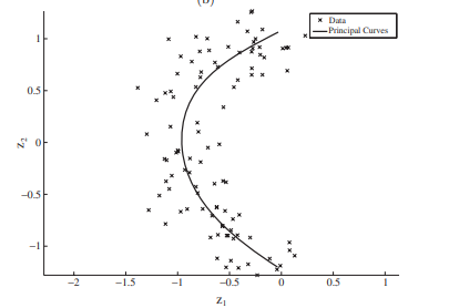
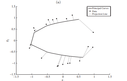
Principal Curves (PCs), presented by Hastie and Stuetzle $[24,25]$, are smooth one-dimensional curves passing through the middle of a cloud representing a data set. Utilizing probability distribution, a principal curve satisfies the self-consistent property, which implies that any point on the curve is the average of all data points projected onto it. As a nonlinear generalization of principal component analysis, $\mathrm{PCs}$ can be also regarded as a one-dimensional manifold embedded in high dimeneional data space. In addition to the sta tistical property inherited from linear principal components, $\mathrm{PCs}$ also reflect the geometrical structure of data due. More precisely, the natural parameter arc-length is regarded as a projection index for each sample in a similar fashion to the score variable that represents the distance of the projected data point from the origin. In this respect, a one-dimensional nonlinear topological relationehip between two variables can be eetimated by a principal curve [85].
统计代写|数据科学代写data science代考|From a weight vector to a principal curve
Inherited from the basic paradigm of $\mathrm{PCA}, \mathrm{PCs}$ assume that the intrinsic middle structure of data is a curve rather than a straight line. In relation to
the total least squares concept $[71]$, the cost function of $\mathrm{PCA}$ is to minimize the sum of projection distances from data points to a line. This produces the same solution as that presented in Sect. 2. Eq. (1.14). Geometrically, eigenvectors and their corresponding eigenvalues of $\mathbf{S}_{Z Z}$ reflect the principal directions and the variance along the principal directions of data, respectively. Applying the above analysis to the first principal component, the following properties can be established [5]:
- Maximize the variance of the projection location of data in the principal directions.
- Minimize the squared distance of the data points from their projections onto the lst principal component.
- Each point of the first principal component is the conditional mean of all data points projected into it.
Assuming the underlying interrelationships between the recorded variables are governed by:
$$
\mathbf{z}=\mathbf{A t}+\mathbf{e},
$$
where $\mathbf{z} \in \mathbb{R}^{N}, \mathbf{t} \in \mathbb{R}^{n}$ is the latent variable (or projection index for the $\mathrm{PCs}$ ), $\mathbf{A} \in \mathbb{R}^{N \times n}$ is a matrix describing the linear interrelationships between data $\mathbf{z}$ and latent variables $\mathbf{t}$, and e represent statistically independent noise, i.e. $E{\mathbf{e}}=\mathbf{0}, E{\mathbf{e e}}=\delta \mathbf{I}, E\left{\mathbf{e t}^{T}\right}=\mathbf{0}$ with $\delta$ being the noise variance. $\mathrm{PCA}$, in this context, uses the above principles of the first principal component to extract the $n$ latent variables $\mathbf{t}$ from a recorded data set $\mathbf{Z}$.
Following from this linear analysis, a general nonlinear form of (1.28) is as follows:
$$
\mathbf{z}=\mathbf{f}(\mathbf{t})+\mathbf{e},
$$
where $\mathbf{f}(\mathbf{t})$ is a nonlinear function and represents the interrelationships between the latent variables $\mathbf{t}$ and the original data $\mathbf{z}$. Reducing $\mathbf{f}(\cdot)$ to be a linear function, Equation (1.29) clearly becomes (1.28), that is a special case of Equation (1.29).
To uncover the intrinsic latent variables, the following cost function, defined as
$$
R=\sum_{i=1}^{K}\left|\mathbf{z}{i}-\mathbf{f}\left(\mathbf{t}{i}\right)\right|_{2}^{2},
$$
where $K$ is the number available observations, can be used.
With respect to (1.30), linear $\mathrm{PCA}$ calculates a vector $\mathbf{p}{1}$ for obtaining the largest projection index $t{i}$ of Equation (1.28), that is the diagonal elements of $E\left{t^{2}\right}$ represent a maximum. Given that $\mathbf{p}{1}$ is of unit length, the location of the projection of $\mathbf{z}{i}$ onto the first principal direction is given by $\mathbf{p}{1} t{i}$. Incorporating a total of $n$ principal directions and utilizing (1.28), Equation (1.30) can be rewritten as follows:
$$
R=\sum_{i=1}^{K}\left|\mathbf{z}{i}-\mathbf{P} \mathbf{t}{i}\right|_{2}^{2}=\operatorname{trace}\left{\mathbf{Z Z}^{T}-\mathbf{Z}^{T} \mathbf{A}\left[\mathbf{A}^{T} \mathbf{A}\right]^{-1} \mathbf{A} \mathbf{Z}^{T}\right}
$$
数据可视化代写
统计代写|数据科学代写data science代考|Nonlinear PCA Extensions
本节回顾了过去二十年来提出的非线性 PCA 扩展。Hastie 和 Stuetzle [25] 提出弯曲载荷矢量以产生近似非线性关系的曲线
一组两个变量。此类曲线被定义为主曲线,将在下一个小节中讨论,包括它们的多维扩展以产生主曲面或主流形。
Kramer [37] 提出的另一种范式与构建人工神经网络有关,以表示 (1.2) 的非线性版本。映射变量集的此类网络和通过定义一个降维瓶颈层,描述非线性主成分,将其定义为自关联神经网络,并在 Subsect 中重新讨论。4.2.
最近提出的 NLPCA 技术涉及定义非线性映射函数以定义特征空间,其中变量空间和假设是这个特征空间的非线性变换。通过使用核函数(例如径向基函数、多项式或 sigmoid 核)仔细选择这些变换,可以构建在概念上和计算上高效的 NLPCA 算法。这种方法,称为 Kermel磷C一种, 在小节中进行了审查。4.3.
统计代写|数据科学代写data science代考|Introduction to principal curves
Hastie 和 Stuetzle 提出的主曲线 (PC)[24,25], 是通过表示数据集的云中间的平滑一维曲线。利用概率分布,主曲线满足自洽性质,这意味着曲线上的任何点都是投影到其上的所有数据点的平均值。作为主成分分析的非线性推广,磷Cs也可以看作是嵌入在高维数据空间中的一维流形。除了继承自线性主成分的统计特性外,磷Cs也反映了数据的几何结构所致。更准确地说,自然参数 arc-length 被视为每个样本的投影索引,其方式类似于表示投影数据点与原点的距离的分数变量。在这方面,两个变量之间的一维非线性拓扑关系可以通过主曲线来估计[85]。
统计代写|数据科学代写data science代考|From a weight vector to a principal curve
继承自基本范式磷C一种,磷Cs假设数据的内在中间结构是曲线而不是直线。和—关联
总最小二乘概念[71], 的成本函数磷C一种是最小化从数据点到直线的投影距离之和。这产生了与 Sect 中提出的解决方案相同的解决方案。2. 等式。(1.14)。在几何上,特征向量及其对应的特征值小号从从分别反映数据的主方向和沿主方向的方差。将上述分析应用于第一主成分,可以建立以下性质[5]:
- 最大化数据在主方向上的投影位置的方差。
- 最小化数据点从它们投影到第一个主成分的平方距离。
- 第一个主成分的每个点都是投影到其中的所有数据点的条件平均值。
假设记录变量之间的潜在相互关系受以下因素支配:
和=一种吨+和,
在哪里和∈Rñ,吨∈Rn是潜在变量(或投影指数磷Cs ), 一种∈Rñ×n是描述数据之间的线性相互关系的矩阵和和潜变量吨, e 表示统计上独立的噪声,即E{\mathbf{e}}=\mathbf{0}, E{\mathbf{e e}}=\delta \mathbf{I}, E\left{\mathbf{e t}^{T}\right}=\数学{0}E{\mathbf{e}}=\mathbf{0}, E{\mathbf{e e}}=\delta \mathbf{I}, E\left{\mathbf{e t}^{T}\right}=\数学{0}和d是噪声方差。磷C一种,在这种情况下,使用上述第一主成分的原理来提取n潜变量吨来自记录的数据集从.
根据该线性分析,(1.28) 的一般非线性形式如下:
和=F(吨)+和,
在哪里F(吨)是一个非线性函数,表示潜在变量之间的相互关系吨和原始数据和. 减少F(⋅)作为一个线性函数,方程(1.29)显然变成了(1.28),这是方程(1.29)的一个特例。
为了揭示内在潜变量,以下成本函数定义为
R=∑一世=1ķ|和一世−F(吨一世)|22,
在哪里ķ是可用观测值的数量,可以使用。
关于 (1.30),线性磷C一种计算一个向量p1获得最大的投影指数吨一世等式(1.28)的对角线元素E\左{t^{2}\右}E\左{t^{2}\右}代表一个最大值。鉴于p1是单位长度,投影的位置和一世在第一个主方向上由下式给出p1吨一世. 共纳入n主要方向和利用(1.28),等式(1.30)可以重写如下:
R=\sum_{i=1}^{K}\left|\mathbf{z}{i}-\mathbf{P} \mathbf{t}{i}\right|_{2}^{2}= \operatorname{trace}\left{\mathbf{Z Z}^{T}-\mathbf{Z}^{T} \mathbf{A}\left[\mathbf{A}^{T} \mathbf{A}\对]^{-1} \mathbf{A} \mathbf{Z}^{T}\right}R=\sum_{i=1}^{K}\left|\mathbf{z}{i}-\mathbf{P} \mathbf{t}{i}\right|_{2}^{2}= \operatorname{trace}\left{\mathbf{Z Z}^{T}-\mathbf{Z}^{T} \mathbf{A}\left[\mathbf{A}^{T} \mathbf{A}\对]^{-1} \mathbf{A} \mathbf{Z}^{T}\right}

统计代写请认准statistics-lab™. statistics-lab™为您的留学生涯保驾护航。统计代写|python代写代考
随机过程代考
在概率论概念中,随机过程是随机变量的集合。 若一随机系统的样本点是随机函数,则称此函数为样本函数,这一随机系统全部样本函数的集合是一个随机过程。 实际应用中,样本函数的一般定义在时间域或者空间域。 随机过程的实例如股票和汇率的波动、语音信号、视频信号、体温的变化,随机运动如布朗运动、随机徘徊等等。
贝叶斯方法代考
贝叶斯统计概念及数据分析表示使用概率陈述回答有关未知参数的研究问题以及统计范式。后验分布包括关于参数的先验分布,和基于观测数据提供关于参数的信息似然模型。根据选择的先验分布和似然模型,后验分布可以解析或近似,例如,马尔科夫链蒙特卡罗 (MCMC) 方法之一。贝叶斯统计概念及数据分析使用后验分布来形成模型参数的各种摘要,包括点估计,如后验平均值、中位数、百分位数和称为可信区间的区间估计。此外,所有关于模型参数的统计检验都可以表示为基于估计后验分布的概率报表。
广义线性模型代考
广义线性模型(GLM)归属统计学领域,是一种应用灵活的线性回归模型。该模型允许因变量的偏差分布有除了正态分布之外的其它分布。
statistics-lab作为专业的留学生服务机构,多年来已为美国、英国、加拿大、澳洲等留学热门地的学生提供专业的学术服务,包括但不限于Essay代写,Assignment代写,Dissertation代写,Report代写,小组作业代写,Proposal代写,Paper代写,Presentation代写,计算机作业代写,论文修改和润色,网课代做,exam代考等等。写作范围涵盖高中,本科,研究生等海外留学全阶段,辐射金融,经济学,会计学,审计学,管理学等全球99%专业科目。写作团队既有专业英语母语作者,也有海外名校硕博留学生,每位写作老师都拥有过硬的语言能力,专业的学科背景和学术写作经验。我们承诺100%原创,100%专业,100%准时,100%满意。
机器学习代写
随着AI的大潮到来,Machine Learning逐渐成为一个新的学习热点。同时与传统CS相比,Machine Learning在其他领域也有着广泛的应用,因此这门学科成为不仅折磨CS专业同学的“小恶魔”,也是折磨生物、化学、统计等其他学科留学生的“大魔王”。学习Machine learning的一大绊脚石在于使用语言众多,跨学科范围广,所以学习起来尤其困难。但是不管你在学习Machine Learning时遇到任何难题,StudyGate专业导师团队都能为你轻松解决。
多元统计分析代考
基础数据: $N$ 个样本, $P$ 个变量数的单样本,组成的横列的数据表
变量定性: 分类和顺序;变量定量:数值
数学公式的角度分为: 因变量与自变量
时间序列分析代写
随机过程,是依赖于参数的一组随机变量的全体,参数通常是时间。 随机变量是随机现象的数量表现,其时间序列是一组按照时间发生先后顺序进行排列的数据点序列。通常一组时间序列的时间间隔为一恒定值(如1秒,5分钟,12小时,7天,1年),因此时间序列可以作为离散时间数据进行分析处理。研究时间序列数据的意义在于现实中,往往需要研究某个事物其随时间发展变化的规律。这就需要通过研究该事物过去发展的历史记录,以得到其自身发展的规律。
回归分析代写
多元回归分析渐进(Multiple Regression Analysis Asymptotics)属于计量经济学领域,主要是一种数学上的统计分析方法,可以分析复杂情况下各影响因素的数学关系,在自然科学、社会和经济学等多个领域内应用广泛。
MATLAB代写
MATLAB 是一种用于技术计算的高性能语言。它将计算、可视化和编程集成在一个易于使用的环境中,其中问题和解决方案以熟悉的数学符号表示。典型用途包括:数学和计算算法开发建模、仿真和原型制作数据分析、探索和可视化科学和工程图形应用程序开发,包括图形用户界面构建MATLAB 是一个交互式系统,其基本数据元素是一个不需要维度的数组。这使您可以解决许多技术计算问题,尤其是那些具有矩阵和向量公式的问题,而只需用 C 或 Fortran 等标量非交互式语言编写程序所需的时间的一小部分。MATLAB 名称代表矩阵实验室。MATLAB 最初的编写目的是提供对由 LINPACK 和 EISPACK 项目开发的矩阵软件的轻松访问,这两个项目共同代表了矩阵计算软件的最新技术。MATLAB 经过多年的发展,得到了许多用户的投入。在大学环境中,它是数学、工程和科学入门和高级课程的标准教学工具。在工业领域,MATLAB 是高效研究、开发和分析的首选工具。MATLAB 具有一系列称为工具箱的特定于应用程序的解决方案。对于大多数 MATLAB 用户来说非常重要,工具箱允许您学习和应用专业技术。工具箱是 MATLAB 函数(M 文件)的综合集合,可扩展 MATLAB 环境以解决特定类别的问题。可用工具箱的领域包括信号处理、控制系统、神经网络、模糊逻辑、小波、仿真等。