如果你也在 怎样代写SLAM这个学科遇到相关的难题，请随时右上角联系我们的24/7代写客服。

同步定位和测绘（SLAM）是构建或更新一个未知环境的地图，同时跟踪一个代理人在其中的位置的计算问题。虽然这最初似乎是一个鸡生蛋蛋生鸡的问题，但有几种已知的算法可以解决这个问题，至少是近似解决，在某些环境下是可行的。流行的近似解决方法包括粒子过滤器、扩展卡尔曼过滤器、协方差交叉和GraphSLAM。SLAM算法是基于计算几何和计算机视觉的概念，并被用于机器人导航、机器人测绘和虚拟现实或增强现实的里程测量。

statistics-lab™ 为您的留学生涯保驾护航 在代写SLAM方面已经树立了自己的口碑, 保证靠谱, 高质且原创的统计Statistics代写服务。我们的专家在代写SLAM代写方面经验极为丰富，各种代写SLAM相关的作业也就用不着说。

我们提供的SLAM及其相关学科的代写，服务范围广, 其中包括但不限于:

• Statistical Inference 统计推断
• Statistical Computing 统计计算
• Advanced Probability Theory 高等概率论
• Advanced Mathematical Statistics 高等数理统计学
• (Generalized) Linear Models 广义线性模型
• Statistical Machine Learning 统计机器学习
• Longitudinal Data Analysis 纵向数据分析
• Foundations of Data Science 数据科学基础

机器人代写|SLAM代写机器人导航代考|Log FastSLAM

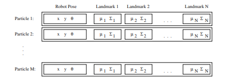
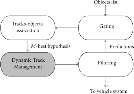
The computational complexity of the FastSLAM algorithm presented up to this point requires time $O(M, N)$ where $M$ is the number of particles, and $N$ is the number of landmarks in the map. The linear complexity in $M$ is unavoidable, given that we have to process $M$ particles for every update. This linear complexity in $N$ is due to the importance resampling step in Section 3.3.4. Since the sampling is done with replacement, a single particle in the weighted particle set may be duplicated several times in $S_{t}$. The simplest way to implement this is to repeatedly copy the entire particle into the new particle set. Since the length of the particles depends linearly on $N$, this copying operation is also linear in the size of the map.

The wholesale copying of particles from the old set into the new set is an overly conservative approach. The majority of the landmark filters remain unchanged at every time step. Indeed, since the sampling is done with replacement, many of the landmark filters will be completely identical.

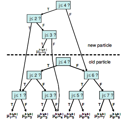
These observations suggest that with proper bookkeeping, a more efficient particle representation might allow duplicate landmark filters to be shared between particles, resulting in a more efficient implementation of FastSLAM. This can be done by changing the particle representation from an array of landmark filters to a binary tree. An example landmark tree is shown in Figure $3.11$ for a map with eight landmarks. In the figure, the landmarks are organized by an arbitrary landmark number $K$. In situations in which data association is unknown, the tree could be organized spatially as in a k-d tree.
Note that the landmark parameters $\mu_{n}, \Sigma_{n}$ are located at the leaves of the tree. Each non-leaf node in the tree contains pointers to up to two subtrees. Any subtree can be shared between multiple particles’ landmark trees. Sharing subtrees makes the update procedure more complicated to implement, but results in a tremendous savings in both memory and computation. Assuming that the tree is balanced, accessing a leaf requires a binary search, which will take $\log (N)$ time, on average.

The $\log (N)$ FastSLAM algorithm can be illustrated by tracing the effect of a control and an observation on the landmark trees. Each new particle in $S_{t}$ will differ from its generating particle in $S_{t-1}$ in two ways. First, each will posses a different pose estimate from (3.17), and second, the observed feature’s Gaussian will be updated as specified in (3.29)-(3.34). All other Gaussians will be equivalent to the generating particle. Thus, when copying the particle to $S_{t}$, only a single path from the root of the tree to the updated Gaussian needs to be duplicated. The length of this path is logarithmic in $N$, on average.
An example is shown in Figure $3.12$. Here we assume that $n_{t}=3$, that is, only the landmark Gaussian parameters $\mu_{3}^{[m]}, \Sigma_{3}^{[m]}$ are updated. Instead of duplicating the entire tree, a single path is duplicated, from the root to the third Gaussian. This path is an incomplete tree. The tree is completed by copying the missing pointers from the tree of the generating particle. Thus, branches that leave the modified path will point to the unmodified subtrees of the generating particle. Clearly, generating this modified tree takes time logarithmic in $N$. Moreover, accessing a Gaussian also takes time logarithmic in $N$, since the number of steps required to navigate to a leaf of the tree is equivalent to the length of the path. Thus, both generating and accessing a partial tree can be done in time $O(\log N)$. $M$ new particles are generated at every update step, so the resulting FastSLAM algorithm requires time $O(M \log N)$.

机器人代写|SLAM代写机器人导航代考|Garbage Collection

Organizing particles as binary trees naturally raises the question of garbage collection. Subtrees are constantly being shared and split between particles. When a subtree is no longer referenced as a part of any particle description,

the memory allocated to this subtree must be freed. Otherwise, the memory required by FastSLAM will grow without bound.

Whenever landmarks are shared between particles, the shared landmarks always form complete subtrees. In other words, if a particular node of the landmark tree is shared between multiple particles, all of the nodes descendants will also be shared. This greatly simplifies garbage collection in FastSLAM, because the landmark trees can be freed recursively.

Garbage collection in FastSLAM can be implemented using reference counts attached to each node in the landmark tree. Each counter counts the number of times the given node is pointed to by other nodes. A newly created node, for example, receives a reference count of 1 . When a new reference is made to a node, the reference count is incremented. When a link is removed, the reference count is decremented. If the reference count reaches zero, the reference counts of the node’s children are decreased, and the node’s memory is freed. This process is then applied recursively to all children of the node with a zero reference count. This process will require $O(M \log N)$ time on average. Furthermore, it is an optimal deallocation algorithm, in that all unneeded memory is freed immediately when it is no longer referenced.

机器人代写|SLAM代写机器人导航代考|Victoria Park

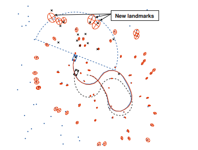
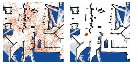
The FastSLAM algorithm was tested on a benchmark SLAM data set from the University of Sydney [37]. An instrumented vehicle, shown in Figure 3.13, equipped with a laser range finder was repeatedly driven through Victoria Park, in Sydney, Australia. Victoria Park is an ideal setting for testing SLAM algorithms because the park’s trees are distinctive features in the robot’s laser scans. Encoders measured the vehicle’s velocity and steering angle. Range and bearing measurements to nearby trees were extracted from the laser data using a local minima detector. The vehicle was driven around for approximately 30 minutes, covering a distance of over $4 \mathrm{~km}$. The vehicle is also equipped with GPS in order to capture ground truth data. Due to occlusion by foliage and buildings, ground truth data is only available for part of the overall traverse. While ground truth is available for the robot’s path, no ground truth data is available for the locations of the landmarks.

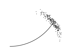
Since the robot is driving over uneven terrain, the measured controls are fairly noisy. Figure $3.14$ (a) shows the path of the robot obtained by integrating the estimated controls. After 30 minutes of driving, the estimated position of the robot is well over 100 meters away from its true position measured by GPS. The laser data, on the other hand, is a very accurate measure of range and bearing. However, not all objects in the robot’s field of view are trees, or even static objects. As a result, the feature detector produced relatively accurate observations of trees, but also generated frequent outliers.

Data association for this experiment was done using per-particle ML data association. Since the accuracy of the observations is high relative to the average density of landmarks, data association in the Victoria Park data set is a relatively straightforward problem. In a later experiment, more difficult data association problems will be simulated by adding extra control noise.
The output of FastSLAM is shown in Figure $3.14(\mathrm{~b})$ and (c). The GPS path is shown as a dashed line, and the output of FastSLAM is shown as a solid line. The RMS error of the resulting path is just over 4 meters over the $4 \mathrm{~km}$ traverse. This experiment was run with 100 particles.

SLAM代写

机器人代写|SLAM代写机器人导航代考|Log FastSLAM

至此提出的 FastSLAM 算法的计算复杂度需要时间这(米,ñ)在哪里米是粒子数，和ñ是地图中地标的数量。线性复杂度米是不可避免的，因为我们必须处理米每次更新的粒子。这种线性复杂度在ñ是由于第 3.3.4 节中的重要性重采样步骤。由于采样是通过替换完成的，因此加权粒子集中的单个粒子可能会在小号吨. 实现这一点的最简单方法是将整个粒子重复复制到新粒子集中。由于粒子的长度线性地取决于ñ，这个复制操作在地图大小上也是线性的。

将旧集合中的粒子批量复制到新集合中是一种过于保守的方法。大多数地标过滤器在每个时间步都保持不变。实际上，由于采样是通过替换完成的，因此许多地标过滤器将完全相同。

这些观察表明，通过适当的簿记，更有效的粒子表示可能允许在粒子之间共享重复的界标过滤器，从而更有效地实现 FastSLAM。这可以通过将粒子表示从地标过滤器数组更改为二叉树来完成。一个示例地标树如图所示3.11一张有八个地标的地图。在图中，地标由任意地标编号组织ķ. 在数据关联未知的情况下，可以像在 kd 树中一样在空间上组织树。
注意地标参数μn,Σn位于树的叶子上。树中的每个非叶节点都包含指向最多两个子树的指针。任何子树都可以在多个粒子的界标树之间共享。共享子树使更新过程的实现更加复杂，但会极大地节省内存和计算量。假设树是平衡的，访问叶子需要二分查找，这将花费日志⁡(ñ)时间，平均而言。

这日志⁡(ñ)FastSLAM 算法可以通过跟踪控制和观察对地标树的影响来说明。每个新粒子小号吨将不同于它的生成粒子小号吨−1有两种方式。首先，每个都将拥有与（3.17）不同的姿态估计，其次，观察到的特征的高斯将按照（3.29）-（3.34）中的规定进行更新。所有其他高斯将等价于生成粒子。因此，当将粒子复制到小号吨，只需要复制从树根到更新的高斯的单个路径。这条路径的长度是对数的ñ， 一般。
一个例子如图所示3.12. 这里我们假设n吨=3，即只有地标高斯参数μ3[米],Σ3[米]被更新。不是复制整个树，而是复制一条路径，从根到第三个高斯。这条路径是一棵不完整的树。通过从生成粒子的树中复制丢失的指针来完成树。因此，离开修改路径的分支将指向生成粒子的未修改子树。显然，生成这个修改过的树需要对数时间ñ. 此外，访问高斯也需要时间对数ñ，因为导航到树的叶子所需的步数等于路径的长度。因此，生成和访问部分树都可以及时完成这(日志⁡ñ). 米每个更新步骤都会生成新粒子，因此生成的 FastSLAM 算法需要时间这(米日志⁡ñ).

机器人代写|SLAM代写机器人导航代考|Garbage Collection

将粒子组织为二叉树自然会引发垃圾收集的问题。子树在粒子之间不断地被共享和分裂。当一个子树不再作为任何粒子描述的一部分被引用时，

必须释放分配给该子树的内存。否则，FastSLAM 所需的内存将无限增长。

每当粒子之间共享界标时，共享界标总是形成完整的子树。换句话说，如果地标树的特定节点在多个粒子之间共享，则所有节点的后代也将被共享。这极大地简化了 FastSLAM 中的垃圾收集，因为可以递归地释放地标树。

FastSLAM 中的垃圾收集可以使用附加到地标树中每个节点的引用计数来实现。每个计数器计算给定节点被其他节点指向的次数。例如，一个新创建的节点接收到的引用计数为 1 。当对节点进行新引用时，引用计数会增加。删除链接时，引用计数会减少。如果引用计数达到零，则该节点的子节点的引用计数减少，并且该节点的内存被释放。然后将此过程递归地应用于具有零引用计数的节点的所有子节点。这个过程将需要这(米日志⁡ñ)平均时间。此外，它是一种最佳的释放算法，因为所有不需要的内存在不再被引用时都会立即释放。

机器人代写|SLAM代写机器人导航代考|Victoria Park

FastSLAM 算法在悉尼大学的基准 SLAM 数据集上进行了测试 [37]。如图 3.13 所示，配备激光测距仪的仪表车辆反复驶过澳大利亚悉尼的维多利亚公园。维多利亚公园是测试 SLAM 算法的理想场所，因为公园的树木是机器人激光扫描的独特特征。编码器测量车辆的速度和转向角。使用局部最小值检测器从激光数据中提取到附近树木的距离和方位测量值。车辆行驶了大约 30 分钟，行驶距离超过4 ķ米. 该车辆还配备了 GPS 以捕获地面实况数据。由于树叶和建筑物的遮挡，地面实况数据仅可用于整个遍历的一部分。虽然地面实况可用于机器人的路径，但没有地面实况数据可用于地标的位置。

由于机器人在不平坦的地形上行驶，因此测量的控制噪声很大。数字3.14(a) 显示了通过集成估计控制获得的机器人路径。行驶 30 分钟后，机器人的估计位置与 GPS 测得的真实位置相差 100 多米。另一方面，激光数据是对距离和方位的非常准确的测量。然而，并非机器人视野中的所有物体都是树木，甚至是静态物体。结果，特征检测器产生了相对准确的树木观察结果，但也产生了频繁的异常值。

该实验的数据关联是使用每粒子 ML 数据关联完成的。由于观测的准确性相对于地标的平均密度较高，因此维多利亚公园数据集中的数据关联是一个相对简单的问题。在以后的实验中，将通过添加额外的控制噪声来模拟更困难的数据关联问题。
FastSLAM的输出如图3.14( b)(c)。GPS路径显示为虚线，FastSLAM的输出显示为实线。所得路径的 RMS 误差仅超过 4 米。4 ķ米遍历。该实验使用 100 个粒子进行。

统计代写请认准statistics-lab™. statistics-lab™为您的留学生涯保驾护航。

金融工程代写

金融工程是使用数学技术来解决金融问题。金融工程使用计算机科学、统计学、经济学和应用数学领域的工具和知识来解决当前的金融问题，以及设计新的和创新的金融产品。

非参数统计代写

非参数统计指的是一种统计方法，其中不假设数据来自于由少数参数决定的规定模型；这种模型的例子包括正态分布模型和线性回归模型。

广义线性模型代考

广义线性模型（GLM）归属统计学领域，是一种应用灵活的线性回归模型。该模型允许因变量的偏差分布有除了正态分布之外的其它分布。

术语 广义线性模型（GLM）通常是指给定连续和/或分类预测因素的连续响应变量的常规线性回归模型。它包括多元线性回归，以及方差分析和方差分析（仅含固定效应）。

有限元方法代写

有限元方法（FEM）是一种流行的方法，用于数值解决工程和数学建模中出现的微分方程。典型的问题领域包括结构分析、传热、流体流动、质量运输和电磁势等传统领域。

有限元是一种通用的数值方法，用于解决两个或三个空间变量的偏微分方程（即一些边界值问题）。为了解决一个问题，有限元将一个大系统细分为更小、更简单的部分，称为有限元。这是通过在空间维度上的特定空间离散化来实现的，它是通过构建对象的网格来实现的：用于求解的数值域，它有有限数量的点。边界值问题的有限元方法表述最终导致一个代数方程组。该方法在域上对未知函数进行逼近。[1] 然后将模拟这些有限元的简单方程组合成一个更大的方程系统，以模拟整个问题。然后，有限元通过变化微积分使相关的误差函数最小化来逼近一个解决方案。

tatistics-lab作为专业的留学生服务机构，多年来已为美国、英国、加拿大、澳洲等留学热门地的学生提供专业的学术服务，包括但不限于Essay代写，Assignment代写，Dissertation代写，Report代写，小组作业代写，Proposal代写，Paper代写，Presentation代写，计算机作业代写，论文修改和润色，网课代做，exam代考等等。写作范围涵盖高中，本科，研究生等海外留学全阶段，辐射金融，经济学，会计学，审计学，管理学等全球99%专业科目。写作团队既有专业英语母语作者，也有海外名校硕博留学生，每位写作老师都拥有过硬的语言能力，专业的学科背景和学术写作经验。我们承诺100%原创，100%专业，100%准时，100%满意。

随机分析代写

随机微积分是数学的一个分支，对随机过程进行操作。它允许为随机过程的积分定义一个关于随机过程的一致的积分理论。这个领域是由日本数学家伊藤清在第二次世界大战期间创建并开始的。

时间序列分析代写

随机过程，是依赖于参数的一组随机变量的全体，参数通常是时间。 随机变量是随机现象的数量表现，其时间序列是一组按照时间发生先后顺序进行排列的数据点序列。通常一组时间序列的时间间隔为一恒定值（如1秒，5分钟，12小时，7天，1年），因此时间序列可以作为离散时间数据进行分析处理。研究时间序列数据的意义在于现实中，往往需要研究某个事物其随时间发展变化的规律。这就需要通过研究该事物过去发展的历史记录，以得到其自身发展的规律。

回归分析代写

多元回归分析渐进（Multiple Regression Analysis Asymptotics）属于计量经济学领域，主要是一种数学上的统计分析方法，可以分析复杂情况下各影响因素的数学关系，在自然科学、社会和经济学等多个领域内应用广泛。

MATLAB代写

MATLAB 是一种用于技术计算的高性能语言。它将计算、可视化和编程集成在一个易于使用的环境中，其中问题和解决方案以熟悉的数学符号表示。典型用途包括：数学和计算算法开发建模、仿真和原型制作数据分析、探索和可视化科学和工程图形应用程序开发，包括图形用户界面构建MATLAB 是一个交互式系统，其基本数据元素是一个不需要维度的数组。这使您可以解决许多技术计算问题，尤其是那些具有矩阵和向量公式的问题，而只需用 C 或 Fortran 等标量非交互式语言编写程序所需的时间的一小部分。MATLAB 名称代表矩阵实验室。MATLAB 最初的编写目的是提供对由 LINPACK 和 EISPACK 项目开发的矩阵软件的轻松访问，这两个项目共同代表了矩阵计算软件的最新技术。MATLAB 经过多年的发展，得到了许多用户的投入。在大学环境中，它是数学、工程和科学入门和高级课程的标准教学工具。在工业领域，MATLAB 是高效研究、开发和分析的首选工具。MATLAB 具有一系列称为工具箱的特定于应用程序的解决方案。对于大多数 MATLAB 用户来说非常重要，工具箱允许您学习和应用专业技术。工具箱是 MATLAB 函数（M 文件）的综合集合，可扩展 MATLAB 环境以解决特定类别的问题。可用工具箱的领域包括信号处理、控制系统、神经网络、模糊逻辑、小波、仿真等。

R语言代写	问卷设计与分析代写
PYTHON代写	回归分析与线性模型代写
MATLAB代写	方差分析与试验设计代写
STATA代写	机器学习/统计学习代写
SPSS代写	计量经济学代写
EVIEWS代写	时间序列分析代写
EXCEL代写	深度学习代写
SQL代写	各种数据建模与可视化代写

如果你也在 怎样代写SLAM这个学科遇到相关的难题，请随时右上角联系我们的24/7代写客服。

同步定位和测绘（SLAM）是构建或更新一个未知环境的地图，同时跟踪一个代理人在其中的位置的计算问题。虽然这最初似乎是一个鸡生蛋蛋生鸡的问题，但有几种已知的算法可以解决这个问题，至少是近似解决，在某些环境下是可行的。流行的近似解决方法包括粒子过滤器、扩展卡尔曼过滤器、协方差交叉和GraphSLAM。SLAM算法是基于计算几何和计算机视觉的概念，并被用于机器人导航、机器人测绘和虚拟现实或增强现实的里程测量。

statistics-lab™ 为您的留学生涯保驾护航 在代写SLAM方面已经树立了自己的口碑, 保证靠谱, 高质且原创的统计Statistics代写服务。我们的专家在代写SLAM代写方面经验极为丰富，各种代写SLAM相关的作业也就用不着说。

我们提供的SLAM及其相关学科的代写，服务范围广, 其中包括但不限于:

• Statistical Inference 统计推断
• Statistical Computing 统计计算
• Advanced Probability Theory 高等概率论
• Advanced Mathematical Statistics 高等数理统计学
• (Generalized) Linear Models 广义线性模型
• Statistical Machine Learning 统计机器学习
• Longitudinal Data Analysis 纵向数据分析
• Foundations of Data Science 数据科学基础

机器人代写|SLAM代写机器人导航代考|Adding New Landmarks

Adding a new landmark to FastSLAM can be difficult decision to make, just as with EKF-based algorithms. This is especially true when an individual measurement is insufficient to constrain the new landmark in all dimensions [13]. If the measurement function $g\left(\theta_{n_{t}}, s_{t}\right)$ is invertible, however, a single measurement is sufficient to initialize a new landmark. Each observation defines a Gaussian:
$$
\mathcal{N}\left(z_{t} ; \hat{z}{t}+G{\theta_{n_{t}}}\left(\theta_{n_{t}}-\mu_{n_{t}, t}^{[m]}\right), R_{t}\right)
$$
This Gaussian can be written explicitly as:
$$
\begin{aligned}
\frac{1}{\sqrt{\left|2 \pi R_{t}\right|}} \exp {&-\frac{1}{2}\left(z_{t}-\hat{z}{t}-G{\theta_{n_{t}}}\left(\theta_{n_{t}}-\mu_{n_{t}, t-1}^{[m]}\right)\right)^{T} \
&\left.R_{t}^{-1}\left(z_{t}-\hat{z}{t}-G{\theta_{n_{t}}}\left(\theta_{n_{t}}-\mu_{n_{t}, t-1}^{[m]}\right)\right)\right}
\end{aligned}
$$
We define a function J to be equal to the negative of the exponent of this Gaussian:
$$
J=\frac{1}{2}\left(z_{t}-\hat{z}{t}-G{\theta_{n_{t}}}\left(\theta_{n_{t}}-\mu_{n_{t}, t-1}^{[m]}\right)\right)^{T} R_{t}^{-1}\left(z_{t}-\hat{z}{t}-G{\theta_{n_{t}}}\left(\theta_{n_{t}}-\mu_{n_{t}, t-1}^{[m]}\right)\right)
$$

The second derivative of $J$ with respect to $\theta_{n_{t}}$ will be the inverse of the covariance matrix of the Gaussian in landmark coordinates.
$$
\begin{aligned}
\frac{\partial J}{\partial \theta_{n_{t}}} &=-\left(z_{t}-\hat{z}{t}-G{\theta_{n_{t}}}\left(\theta_{n_{t}}-\mu_{n_{t}, t-1}^{[m]}\right)\right)^{T} R_{t}^{-1} G_{\theta_{n_{t}}} \
\frac{\partial^{2} J}{\partial \theta_{n_{t}}^{2}} &=G_{\theta_{n_{t}}}^{T} R_{t}^{-1} G_{\theta_{n_{t}}}
\end{aligned}
$$
Consequently, an invertible observation can be used to create a new landmark as follows.
$$
\begin{aligned}
\mu_{n_{t}, t}^{[m]} &=g^{-1}\left(s_{t}^{[m]}, z_{t}\right) \
\Sigma_{n_{t}, t}^{[m]} &=\left(G_{\theta_{n_{t}}, t}^{T} R^{-1} G_{\theta_{n_{t}}, t}\right)^{-1} \
w_{t}^{[m]} &=p_{0}
\end{aligned}
$$
In practice, a simpler initialization procedure also works well. Instead of computing the correct initial covariance, the covariance can be computed by setting the variance of each landmark parameter to a large initial value $K$ and incorporating the first observation. Higher values of $K$ lead to closer approximations of the true covariance, but can also lead to numerical instability.
$$
\begin{aligned}
\mu_{n_{t}, t}^{[m]} &=g^{-1}\left(s_{t}^{[m]}, z_{t}\right) \
\Sigma_{n_{t}, t}^{[m]} &=K \cdot I
\end{aligned}
$$
Initialization techniques for situations in which $g$ is not invertible (e.g. bearings-only SLAM) are discussed in $[12,13]$. These situations require the accumulation of multiple observations in order to estimate the location of a landmark. FastSLAM is currently being applied to the problem of bearingsonly SLAM [83].

机器人代写|SLAM代写机器人导航代考|Summary of the FastSLAM Algorithm

Table $3.2$ summarizes the FastSLAM algorithm with unknown data association. Particles in the complete FastSLAM algorithm have the form:
$$
S_{t}^{[m]}=\left\langle s_{t}^{[m]} \mid N_{t}^{[m]}, \mu_{1, t}^{[m]}, \Sigma_{1, t}^{[m]}, \ldots, \mu_{N_{t}^{[m]}, t}^{[m]}, \Sigma_{N_{t}^{[m]}, t}^{[m]}\right\rangle
$$
In addition to the latest robot pose $s_{t}^{[m]}$ and the feature estimates $\mu_{n, t}^{[m]}$ and $\Sigma_{n, t}^{[m]}$, each particle maintains the number of features $N_{t}^{[m]}$ in its local map. It is interesting to note that each particle may have a different number of landmarks. This is an expressive representation, but it can lead to difficulties in determining the most probable map.

机器人代写|SLAM代写机器人导航代考|Greedy Mutual Exclusion

If multiple observations are incorporated simultaneously, the simplest approach to data association is to consider the identity of each observation independently. However, the data associations of each observation are clearly correlated, as was shown in Section 3.4. The data associations are correlated

through error in the robot pose, and they also must all obey a mutual exclusion constraint; more than one observation cannot be associated with the same landmark at the same time. Considering the data associations jointly does address these problems $[1,14,68]$, but these techniques are computationally expensive for large numbers of simultaneous observations.

FastSLAM addresses the first problem, motion ambiguity, by sampling over robot poses and data associations. Each set of data association decisions is conditioned on a particular robot path. Thus, the data associations can be chosen independently without fear that pose error will corrupt all of the decisions. Some of the particles will chose the correct data associations, while others draw inconsistent robot poses, pick incorrect data associations, and receive low weights. Picking associations independently per particle still ignores the issue of mutual exclusion, however. Mutual exclusion is particularly useful for deciding when to add new landmarks in noisy environments. Instead of assigning an observation of an unseen landmark to an existing landmark, mutual exclusion will force the creation of a new landmark if both features are observed.

Proper handling of mutual exclusion requires that the data associations of all observations be considered simultaneously. However, mutual exclusion can also be enforced in a greedy fashion. Each observation is processed sequentially and ignores the landmarks associated with previously assigned observations. With a single data association hypothesis, applying mutual exclusion greedily can lead to failures in noisy environments. It can work well in FastSLAM, though, because the motion ambiguity that commonly causes greedy mutual exclusion failures is largely factored out by sampling over the the robot’s path. Furthermore, errors due to the greedy nature of the algorithm can also be minimized by processing the observations in different orders for each particle.

SLAM代写

机器人代写|SLAM代写机器人导航代考|Adding New Landmarks

与基于 EKF 的算法一样，向 FastSLAM 添加新的地标可能是一个艰难的决定。当单个测量不足以在所有维度上约束新地标时尤其如此 [13]。如果测量功能G(θn吨,s吨)是可逆的，然而，一次测量就足以初始化一个新的地标。每个观察定义一个高斯：
ñ(和吨;和^吨+Gθn吨(θn吨−μn吨,吨[米]),R吨)
这个高斯分布可以明确地写成：
\begin{aligned} \frac{1}{\sqrt{\left|2 \pi R_{t}\right|}} \exp {&-\frac{1}{2}\left(z_{t}- \hat{z}{t}-G{\theta_{n_{t}}}\left(\theta_{n_{t}}-\mu_{n_{t}, t-1}^{[m]} \right)\right)^{T} \ &\left.R_{t}^{-1}\left(z_{t}-\hat{z}{t}-G{\theta_{n_{t} }}\left(\theta_{n_{t}}-\mu_{n_{t}, t-1}^{[m]}\right)\right)\right} \end{aligned}\begin{aligned} \frac{1}{\sqrt{\left|2 \pi R_{t}\right|}} \exp {&-\frac{1}{2}\left(z_{t}- \hat{z}{t}-G{\theta_{n_{t}}}\left(\theta_{n_{t}}-\mu_{n_{t}, t-1}^{[m]} \right)\right)^{T} \ &\left.R_{t}^{-1}\left(z_{t}-\hat{z}{t}-G{\theta_{n_{t} }}\left(\theta_{n_{t}}-\mu_{n_{t}, t-1}^{[m]}\right)\right)\right} \end{aligned}
我们定义一个函数 J 等于这个高斯指数的负数：
Ĵ=12(和吨−和^吨−Gθn吨(θn吨−μn吨,吨−1[米]))吨R吨−1(和吨−和^吨−Gθn吨(θn吨−μn吨,吨−1[米]))

的二阶导数Ĵ关于θn吨将是高斯在地标坐标中的协方差矩阵的逆。
∂Ĵ∂θn吨=−(和吨−和^吨−Gθn吨(θn吨−μn吨,吨−1[米]))吨R吨−1Gθn吨 ∂2Ĵ∂θn吨2=Gθn吨吨R吨−1Gθn吨
因此，可以使用可逆观察来创建新的地标，如下所示。
μn吨,吨[米]=G−1(s吨[米],和吨) Σn吨,吨[米]=(Gθn吨,吨吨R−1Gθn吨,吨)−1 在吨[米]=p0
在实践中，更简单的初始化过程也可以很好地工作。可以通过将每个地标参数的方差设置为较大的初始值来计算协方差，而不是计算正确的初始协方差ķ并结合第一个观察结果。较高的值ķ导致更接近真实协方差，但也可能导致数值不稳定。
μn吨,吨[米]=G−1(s吨[米],和吨) Σn吨,吨[米]=ķ⋅一世
针对以下情况的初始化技术G是不可逆的（例如仅轴承 SLAM）在[12,13]. 这些情况需要累积多个观测值以估计地标的位置。FastSLAM 目前正在应用于仅轴承问题的 SLAM [83]。

机器人代写|SLAM代写机器人导航代考|Summary of the FastSLAM Algorithm

桌子3.2总结了未知数据关联的FastSLAM算法。完整的 FastSLAM 算法中的粒子具有以下形式：
小号吨[米]=⟨s吨[米]∣ñ吨[米],μ1,吨[米],Σ1,吨[米],…,μñ吨[米],吨[米],Σñ吨[米],吨[米]⟩
除了最新的机器人姿势s吨[米]和特征估计μn,吨[米]和Σn,吨[米]，每个粒子保持特征的数量ñ吨[米]在其本地地图中。有趣的是，每个粒子可能有不同数量的界标。这是一种富有表现力的表示，但它可能会导致难以确定最可能的地图。

机器人代写|SLAM代写机器人导航代考|Greedy Mutual Exclusion

如果同时合并多个观察，最简单的数据关联方法是独立考虑每个观察的身份。然而，每个观察的数据关联显然是相关的，如第 3.4 节所示。数据关联是相关的

由于机器人姿态的错误，它们也必须都服从互斥约束；一个以上的观察不能同时与同一个地标相关联。联合考虑数据关联确实解决了这些问题[1,14,68]，但这些技术对于大量同时观察的计算成本很高。

FastSLAM 通过对机器人姿势和数据关联进行采样来解决第一个问题，即运动模糊性。每组数据关联决策都以特定的机器人路径为条件。因此，可以独立选择数据关联，而不必担心姿势错误会破坏所有决策。一些粒子会选择正确的数据关联，而其他粒子会绘制不一致的机器人姿势，选择不正确的数据关联，并获得低权重。然而，每个粒子独立地选择关联仍然忽略了互斥问题。互斥对于决定何时在嘈杂环境中添加新地标特别有用。如果两个特征都被观察到，互斥将强制创建新的地标，而不是将未见地标的观察分配给现有地标。

正确处理互斥需要同时考虑所有观察值的数据关联。但是，互斥也可以以贪婪的方式强制执行。每个观察都按顺序处理，并忽略与先前分配的观察相关的界标。对于单一的数据关联假设，贪婪地应用互斥可能会导致在嘈杂环境中失败。不过，它可以在 FastSLAM 中很好地工作，因为通常会导致贪婪互斥失败的运动模糊性在很大程度上是通过对机器人路径的采样来排除的。此外，由于算法的贪心性质导致的错误也可以通过以不同顺序处理每个粒子的观察结果来最小化。

统计代写请认准statistics-lab™. statistics-lab™为您的留学生涯保驾护航。

金融工程代写

金融工程是使用数学技术来解决金融问题。金融工程使用计算机科学、统计学、经济学和应用数学领域的工具和知识来解决当前的金融问题，以及设计新的和创新的金融产品。

非参数统计代写

非参数统计指的是一种统计方法，其中不假设数据来自于由少数参数决定的规定模型；这种模型的例子包括正态分布模型和线性回归模型。

广义线性模型代考

广义线性模型（GLM）归属统计学领域，是一种应用灵活的线性回归模型。该模型允许因变量的偏差分布有除了正态分布之外的其它分布。

术语 广义线性模型（GLM）通常是指给定连续和/或分类预测因素的连续响应变量的常规线性回归模型。它包括多元线性回归，以及方差分析和方差分析（仅含固定效应）。

有限元方法代写

有限元方法（FEM）是一种流行的方法，用于数值解决工程和数学建模中出现的微分方程。典型的问题领域包括结构分析、传热、流体流动、质量运输和电磁势等传统领域。

有限元是一种通用的数值方法，用于解决两个或三个空间变量的偏微分方程（即一些边界值问题）。为了解决一个问题，有限元将一个大系统细分为更小、更简单的部分，称为有限元。这是通过在空间维度上的特定空间离散化来实现的，它是通过构建对象的网格来实现的：用于求解的数值域，它有有限数量的点。边界值问题的有限元方法表述最终导致一个代数方程组。该方法在域上对未知函数进行逼近。[1] 然后将模拟这些有限元的简单方程组合成一个更大的方程系统，以模拟整个问题。然后，有限元通过变化微积分使相关的误差函数最小化来逼近一个解决方案。

tatistics-lab作为专业的留学生服务机构，多年来已为美国、英国、加拿大、澳洲等留学热门地的学生提供专业的学术服务，包括但不限于Essay代写，Assignment代写，Dissertation代写，Report代写，小组作业代写，Proposal代写，Paper代写，Presentation代写，计算机作业代写，论文修改和润色，网课代做，exam代考等等。写作范围涵盖高中，本科，研究生等海外留学全阶段，辐射金融，经济学，会计学，审计学，管理学等全球99%专业科目。写作团队既有专业英语母语作者，也有海外名校硕博留学生，每位写作老师都拥有过硬的语言能力，专业的学科背景和学术写作经验。我们承诺100%原创，100%专业，100%准时，100%满意。

随机分析代写

随机微积分是数学的一个分支，对随机过程进行操作。它允许为随机过程的积分定义一个关于随机过程的一致的积分理论。这个领域是由日本数学家伊藤清在第二次世界大战期间创建并开始的。

时间序列分析代写

随机过程，是依赖于参数的一组随机变量的全体，参数通常是时间。 随机变量是随机现象的数量表现，其时间序列是一组按照时间发生先后顺序进行排列的数据点序列。通常一组时间序列的时间间隔为一恒定值（如1秒，5分钟，12小时，7天，1年），因此时间序列可以作为离散时间数据进行分析处理。研究时间序列数据的意义在于现实中，往往需要研究某个事物其随时间发展变化的规律。这就需要通过研究该事物过去发展的历史记录，以得到其自身发展的规律。

回归分析代写

多元回归分析渐进（Multiple Regression Analysis Asymptotics）属于计量经济学领域，主要是一种数学上的统计分析方法，可以分析复杂情况下各影响因素的数学关系，在自然科学、社会和经济学等多个领域内应用广泛。

MATLAB代写

MATLAB 是一种用于技术计算的高性能语言。它将计算、可视化和编程集成在一个易于使用的环境中，其中问题和解决方案以熟悉的数学符号表示。典型用途包括：数学和计算算法开发建模、仿真和原型制作数据分析、探索和可视化科学和工程图形应用程序开发，包括图形用户界面构建MATLAB 是一个交互式系统，其基本数据元素是一个不需要维度的数组。这使您可以解决许多技术计算问题，尤其是那些具有矩阵和向量公式的问题，而只需用 C 或 Fortran 等标量非交互式语言编写程序所需的时间的一小部分。MATLAB 名称代表矩阵实验室。MATLAB 最初的编写目的是提供对由 LINPACK 和 EISPACK 项目开发的矩阵软件的轻松访问，这两个项目共同代表了矩阵计算软件的最新技术。MATLAB 经过多年的发展，得到了许多用户的投入。在大学环境中，它是数学、工程和科学入门和高级课程的标准教学工具。在工业领域，MATLAB 是高效研究、开发和分析的首选工具。MATLAB 具有一系列称为工具箱的特定于应用程序的解决方案。对于大多数 MATLAB 用户来说非常重要，工具箱允许您学习和应用专业技术。工具箱是 MATLAB 函数（M 文件）的综合集合，可扩展 MATLAB 环境以解决特定类别的问题。可用工具箱的领域包括信号处理、控制系统、神经网络、模糊逻辑、小波、仿真等。

R语言代写	问卷设计与分析代写
PYTHON代写	回归分析与线性模型代写
MATLAB代写	方差分析与试验设计代写
STATA代写	机器学习/统计学习代写
SPSS代写	计量经济学代写
EVIEWS代写	时间序列分析代写
EXCEL代写	深度学习代写
SQL代写	各种数据建模与可视化代写

如果你也在 怎样代写SLAM这个学科遇到相关的难题，请随时右上角联系我们的24/7代写客服。

同步定位和测绘（SLAM）是构建或更新一个未知环境的地图，同时跟踪一个代理人在其中的位置的计算问题。虽然这最初似乎是一个鸡生蛋蛋生鸡的问题，但有几种已知的算法可以解决这个问题，至少是近似解决，在某些环境下是可行的。流行的近似解决方法包括粒子过滤器、扩展卡尔曼过滤器、协方差交叉和GraphSLAM。SLAM算法是基于计算几何和计算机视觉的概念，并被用于机器人导航、机器人测绘和虚拟现实或增强现实的里程测量。

statistics-lab™ 为您的留学生涯保驾护航 在代写SLAM方面已经树立了自己的口碑, 保证靠谱, 高质且原创的统计Statistics代写服务。我们的专家在代写SLAM代写方面经验极为丰富，各种代写SLAM相关的作业也就用不着说。

我们提供的SLAM及其相关学科的代写，服务范围广, 其中包括但不限于:

• Statistical Inference 统计推断
• Statistical Computing 统计计算
• Advanced Probability Theory 高等概率论
• Advanced Mathematical Statistics 高等数理统计学
• (Generalized) Linear Models 广义线性模型
• Statistical Machine Learning 统计机器学习
• Longitudinal Data Analysis 纵向数据分析
• Foundations of Data Science 数据科学基础

机器人代写|SLAM代写机器人导航代考|FastSLAM with Unknown Data Association

The biggest limitation of the FastSLAM algorithm described thus far is the assumption that the data associations $n^{t}$ are known. In practice, this is rarely the case. This section extends the FastSLAM algorithm to domains in which the mapping between observations and landmarks is not known [57]. The classical solution to the data association problem in SLAM is to chose $n_{t}$ such that it maximizes the likelihood of the sensor measurement $z_{t}$ given all available data [18].
$$
\hat{n}{t}=\underset{n{t}}{\operatorname{argmax}} p\left(z_{t} \mid n_{t}, \hat{n}^{t-1}, s^{t}, z^{t-1}, u^{t}\right)
$$
The term $p\left(z_{t} \mid n_{t}, \hat{n}^{t-1}, s^{t}, z^{t-1}, u^{t}\right)$ is referred to as a likelihood, and this approach is an example of a maximum likelihood (ML) estimator. ML data association is also called “nearest neighbor” data association, interpreting the negative log likelihood as a distance function. For Gaussians, the negative log likelihood is Mahalanobis distance, and the estimator selects data associations by minimizing this Mahalanobis distance.

In the EKF-based SLAM approaches described in Chapter 2, a single data association is chosen for the entire filter. As a result, these algorithms tend to be brittle to failures in data association. A single data association error can induce significant errors in the map, which in turn cause new data association errors, often with fatal consequences. A better understanding of how uncertainty in the SLAM posterior generates data association ambiguity will demonstrate how simple data association heuristics often fail.

机器人代写|SLAM代写机器人导航代考|Data Association Uncertainty

Two factors contribute to uncertainty in the SLAM posterior: measurement noise and motion noise. As measurement noise increases, the distributions of possible observations of every landmark become more uncertain. If measurement noise is sufficiently high, the distributions of observations from nearby landmarks will begin to overlap substantially. This overlap leads to ambiguity

in the identity of the landmarks. We will refer to data association ambiguity caused by measurement noise as measurement ambiguity. An example of measurement ambiguity is shown in Figure 3.7. The two ellipses depict the range of probable observations from two different landmarks. The observation, shown as an black circle, plausibly could have come from either landmark.
Attributing an observation to the wrong landmark due to measurement ambiguity will increase the error of the map and robot pose, but its impact will be relatively minor. Since the observation could have been generated by either landmark with high probability, the effect of the observation on the landmark positions and the robot pose will be small. The covariance of one landmark will be slightly overestimated, while the covariance of the second will be slightly underestimated. If multiple observations are incorporated per control, a data association mistake due to measurement ambiguity of one observation will have relatively little impact on the data association decisions for the other observations.

Ambiguity in data association caused by motion noise can have much more severe consequences on estimation accuracy. Higher motion noise will lead to higher pose uncertainty after incorporating a control. If this pose uncertainty is high enough, assuming different robot poses in this distribution will imply drastically different ML data association hypotheses for the subsequent observations. This motion ambiguity, shown in Figure $3.8$, is easily induced if there is significant rotational error in the robot’s motion. Moreover, if multiple observations are incorporated per control, the pose of the robot will correlate the data association decisions of all of the observations. If the SLAM algorithm chooses the wrong data association for a single observation due to motion ambiguity, the rest of the data associations also will be wrong with high probability.

机器人代写|SLAM代写机器人导航代考|Per-Particle Data Association

Unlike most EKF-based SLAM algorithms, FastSLAM takes a multi-hypothesis approach to the data association problem. Each particle represents a different hypothesized path of the robot, so data association decisions can be made on a per-particle basis. Particles that pick the correct data association will receive high weights because they explain the observations well. Particles that pick wrong associations will receive low weights and be removed in a future resampling step.

Per-particle data association has several important advantages over standard ML data association. First, it factors robot pose uncertainty out of the data association problem. Since motion ambiguity is the more severe form of data association ambiguity, conditioning the data association decisions on hypothesized robot paths seems like a logical choice. Given the scenario in Figure 3.8, some of the particles would draw new robot poses consistent with data association hypothesis on the left, while others would draw poses consistent with the data association hypothesis on the right.

Doing data association on a per-particle basis also makes the data association problem easier. In the EKF, the uncertainty of a landmark position is due to both uncertainty in the pose of the robot and measurement error. In FastSLAM, uncertainty of the robot pose is represented by the entire particle set. The landmark filters in a single particle are not affected by motion noise because they are conditioned on a specific robot path. This is especially useful if the robot has noisy motion and an accurate sensor.

Another consequence of per-particle data association is implicit, delayeddecision making. At any given time, some fraction of the particles will receive plausible, yet wrong, data associations. In the future, the robot may receive a new observation that clearly refutes these previous assignments. At this point, the particles with wrong data associations will receive low weight and likely be removed from the filter. As a result of this process, the effect of a wrong data association decision made in the past can be removed from the filter. Moreover, no heuristics are needed in order to remove incorrect old associations from the filter. This is done in a statistically valid manner, simply as a consequence of the resampling step.

SLAM代写

机器人代写|SLAM代写机器人导航代考|FastSLAM with Unknown Data Association

迄今为止描述的 FastSLAM 算法的最大限制是假设数据关联n吨是已知的。在实践中，这种情况很少见。本节将 FastSLAM 算法扩展到观察值和地标之间的映射未知的领域 [57]。SLAM中数据关联问题的经典解决方案是选择n吨使其最大化传感器测量的可能性和吨给定所有可用数据[18]。
n^吨=最大参数n吨p(和吨∣n吨,n^吨−1,s吨,和吨−1,在吨)
术语p(和吨∣n吨,n^吨−1,s吨,和吨−1,在吨)被称为似然性，这种方法是最大似然（ML）估计器的一个例子。ML 数据关联也称为“最近邻”数据关联，将负对数似然解释为距离函数。对于高斯，负对数似然是马氏距离，估计器通过最小化这个马氏距离来选择数据关联。

在第 2 章描述的基于 EKF 的 SLAM 方法中，为整个过滤器选择单个数据关联。因此，这些算法往往会因数据关联失败而变得脆弱。单个数据关联错误可能会在地图中引发重大错误，进而导致新的数据关联错误，通常会带来致命的后果。更好地理解 SLAM 后验中的不确定性如何产生数据关联模糊性将证明简单的数据关联启发式方法经常失败。

机器人代写|SLAM代写机器人导航代考|Data Association Uncertainty

有两个因素会导致 SLAM 后验的不确定性：测量噪声和运动噪声。随着测量噪声的增加，每个地标的可能观测值的分布变得更加不确定。如果测量噪声足够高，来自附近地标的观测分布将开始大量重叠。这种重叠导致歧义

在地标的身份中。我们将由测量噪声引起的数据关联模糊度称为测量模糊度。图 3.7 显示了测量模糊度的一个示例。这两个椭圆描绘了来自两个不同地标的可能观测值的范围。显示为黑色圆圈的观察结果很可能来自任一地标。
由于测量模糊而将观察归因于错误的地标会增加地图和机器人位姿的误差，但其影响相对较小。由于观测可能是由任一界标产生的概率很高，因此观测对界标位置和机器人姿态的影响将很小。一个地标的协方差会被略微高估，而第二个地标的协方差会被略微低估。如果每个控制包含多个观察，则由于一个观察的测量模糊性导致的数据关联错误对其他观察的数据关联决策的影响相对较小。

由运动噪声引起的数据关联模糊会对估计精度产生更严重的影响。结合控制后，更高的运动噪声将导致更高的姿势不确定性。如果此姿势不确定性足够高，则假设此分布中的不同机器人姿势将意味着后续观察的 ML 数据关联假设大不相同。这种运动模糊，如图3.8, 如果机器人运动中存在明显的旋转误差，则很容易引起。此外，如果每个控件包含多个观测值，机器人的姿势将关联所有观测值的数据关联决策。如果 SLAM 算法由于运动模糊而为单个观察选择了错误的数据关联，那么其余数据关联也很有可能是错误的。

机器人代写|SLAM代写机器人导航代考|Per-Particle Data Association

与大多数基于 EKF 的 SLAM 算法不同，FastSLAM 对数据关联问题采用多假设方法。每个粒子代表机器人的不同假设路径，因此可以在每个粒子的基础上做出数据关联决策。选择正确数据关联的粒子将获得高权重，因为它们很好地解释了观察结果。选择错误关联的粒子将获得较低的权重，并在未来的重采样步骤中被移除。

与标准 ML 数据关联相比，每粒子数据关联具有几个重要优势。首先，它将机器人姿态不确定性排除在数据关联问题之外。由于运动模糊是数据关联模糊的更严重形式，因此根据假设的机器人路径调整数据关联决策似乎是一个合乎逻辑的选择。给定图 3.8 中的场景，一些粒子将绘制与左侧数据关联假设一致的新机器人姿态，而其他粒子将绘制与右侧数据关联假设一致的姿态。

在每个粒子的基础上进行数据关联也使数据关联问题更容易。在 EKF 中，地标位置的不确定性是由于机器人位姿的不确定性和测量误差造成的。在 FastSLAM 中，机器人姿态的不确定性由整个粒子集表示。单个粒子中的界标滤波器不受运动噪声的影响，因为它们以特定的机器人路径为条件。如果机器人有嘈杂的运动和准确的传感器，这将特别有用。

每粒子数据关联的另一个结果是隐含的、延迟的决策制定。在任何给定时间，一部分粒子都会收到似是而非的数据关联。将来，机器人可能会收到一个新的观察结果，该观察结果清楚地反驳了这些先前的任务。此时，具有错误数据关联的粒子将获得较低的权重，并可能从过滤器中移除。作为这个过程的结果，过去做出的错误数据关联决策的影响可以从过滤器中移除。此外，不需要启发式方法来从过滤器中删除不正确的旧关联。这是以统计上有效的方式完成的，只是作为重采样步骤的结果。

统计代写请认准statistics-lab™. statistics-lab™为您的留学生涯保驾护航。

金融工程代写

金融工程是使用数学技术来解决金融问题。金融工程使用计算机科学、统计学、经济学和应用数学领域的工具和知识来解决当前的金融问题，以及设计新的和创新的金融产品。

非参数统计代写

非参数统计指的是一种统计方法，其中不假设数据来自于由少数参数决定的规定模型；这种模型的例子包括正态分布模型和线性回归模型。

广义线性模型代考

广义线性模型（GLM）归属统计学领域，是一种应用灵活的线性回归模型。该模型允许因变量的偏差分布有除了正态分布之外的其它分布。

术语 广义线性模型（GLM）通常是指给定连续和/或分类预测因素的连续响应变量的常规线性回归模型。它包括多元线性回归，以及方差分析和方差分析（仅含固定效应）。

有限元方法代写

有限元方法（FEM）是一种流行的方法，用于数值解决工程和数学建模中出现的微分方程。典型的问题领域包括结构分析、传热、流体流动、质量运输和电磁势等传统领域。

有限元是一种通用的数值方法，用于解决两个或三个空间变量的偏微分方程（即一些边界值问题）。为了解决一个问题，有限元将一个大系统细分为更小、更简单的部分，称为有限元。这是通过在空间维度上的特定空间离散化来实现的，它是通过构建对象的网格来实现的：用于求解的数值域，它有有限数量的点。边界值问题的有限元方法表述最终导致一个代数方程组。该方法在域上对未知函数进行逼近。[1] 然后将模拟这些有限元的简单方程组合成一个更大的方程系统，以模拟整个问题。然后，有限元通过变化微积分使相关的误差函数最小化来逼近一个解决方案。

tatistics-lab作为专业的留学生服务机构，多年来已为美国、英国、加拿大、澳洲等留学热门地的学生提供专业的学术服务，包括但不限于Essay代写，Assignment代写，Dissertation代写，Report代写，小组作业代写，Proposal代写，Paper代写，Presentation代写，计算机作业代写，论文修改和润色，网课代做，exam代考等等。写作范围涵盖高中，本科，研究生等海外留学全阶段，辐射金融，经济学，会计学，审计学，管理学等全球99%专业科目。写作团队既有专业英语母语作者，也有海外名校硕博留学生，每位写作老师都拥有过硬的语言能力，专业的学科背景和学术写作经验。我们承诺100%原创，100%专业，100%准时，100%满意。

随机分析代写

随机微积分是数学的一个分支，对随机过程进行操作。它允许为随机过程的积分定义一个关于随机过程的一致的积分理论。这个领域是由日本数学家伊藤清在第二次世界大战期间创建并开始的。

时间序列分析代写

随机过程，是依赖于参数的一组随机变量的全体，参数通常是时间。 随机变量是随机现象的数量表现，其时间序列是一组按照时间发生先后顺序进行排列的数据点序列。通常一组时间序列的时间间隔为一恒定值（如1秒，5分钟，12小时，7天，1年），因此时间序列可以作为离散时间数据进行分析处理。研究时间序列数据的意义在于现实中，往往需要研究某个事物其随时间发展变化的规律。这就需要通过研究该事物过去发展的历史记录，以得到其自身发展的规律。

回归分析代写

多元回归分析渐进（Multiple Regression Analysis Asymptotics）属于计量经济学领域，主要是一种数学上的统计分析方法，可以分析复杂情况下各影响因素的数学关系，在自然科学、社会和经济学等多个领域内应用广泛。

MATLAB代写

MATLAB 是一种用于技术计算的高性能语言。它将计算、可视化和编程集成在一个易于使用的环境中，其中问题和解决方案以熟悉的数学符号表示。典型用途包括：数学和计算算法开发建模、仿真和原型制作数据分析、探索和可视化科学和工程图形应用程序开发，包括图形用户界面构建MATLAB 是一个交互式系统，其基本数据元素是一个不需要维度的数组。这使您可以解决许多技术计算问题，尤其是那些具有矩阵和向量公式的问题，而只需用 C 或 Fortran 等标量非交互式语言编写程序所需的时间的一小部分。MATLAB 名称代表矩阵实验室。MATLAB 最初的编写目的是提供对由 LINPACK 和 EISPACK 项目开发的矩阵软件的轻松访问，这两个项目共同代表了矩阵计算软件的最新技术。MATLAB 经过多年的发展，得到了许多用户的投入。在大学环境中，它是数学、工程和科学入门和高级课程的标准教学工具。在工业领域，MATLAB 是高效研究、开发和分析的首选工具。MATLAB 具有一系列称为工具箱的特定于应用程序的解决方案。对于大多数 MATLAB 用户来说非常重要，工具箱允许您学习和应用专业技术。工具箱是 MATLAB 函数（M 文件）的综合集合，可扩展 MATLAB 环境以解决特定类别的问题。可用工具箱的领域包括信号处理、控制系统、神经网络、模糊逻辑、小波、仿真等。

R语言代写	问卷设计与分析代写
PYTHON代写	回归分析与线性模型代写
MATLAB代写	方差分析与试验设计代写
STATA代写	机器学习/统计学习代写
SPSS代写	计量经济学代写
EVIEWS代写	时间序列分析代写
EXCEL代写	深度学习代写
SQL代写	各种数据建模与可视化代写

如果你也在 怎样代写SLAM这个学科遇到相关的难题，请随时右上角联系我们的24/7代写客服。

同步定位和测绘（SLAM）是构建或更新一个未知环境的地图，同时跟踪一个代理人在其中的位置的计算问题。虽然这最初似乎是一个鸡生蛋蛋生鸡的问题，但有几种已知的算法可以解决这个问题，至少是近似解决，在某些环境下是可行的。流行的近似解决方法包括粒子过滤器、扩展卡尔曼过滤器、协方差交叉和GraphSLAM。SLAM算法是基于计算几何和计算机视觉的概念，并被用于机器人导航、机器人测绘和虚拟现实或增强现实的里程测量。

statistics-lab™ 为您的留学生涯保驾护航 在代写SLAM方面已经树立了自己的口碑, 保证靠谱, 高质且原创的统计Statistics代写服务。我们的专家在代写SLAM代写方面经验极为丰富，各种代写SLAM相关的作业也就用不着说。

我们提供的SLAM及其相关学科的代写，服务范围广, 其中包括但不限于:

• Statistical Inference 统计推断
• Statistical Computing 统计计算
• Advanced Probability Theory 高等概率论
• Advanced Mathematical Statistics 高等数理统计学
• (Generalized) Linear Models 广义线性模型
• Statistical Machine Learning 统计机器学习
• Longitudinal Data Analysis 纵向数据分析
• Foundations of Data Science 数据科学基础

机器人代写|SLAM代写机器人导航代考|Updating the Landmark Estimates

FastSLAM represents the conditional landmark estimates $p\left(\theta_{n} \mid s^{t}, z^{t}, u^{t}, n^{t}\right)$ in (3.3) using low-dimensional EKFs. For now, I will assume that the data associations $n^{t}$ are known. In section 3.4, this restriction will be removed.
Since the landmark estimates are conditioned on the robot’s path, $N$ EKFs are attached to each particle in $S_{t}$. The posterior over the $n$-th landmark position $\theta_{n}$ is easily obtained. Its computation depends on whether $n=n_{t}$, that is, whether or not landmark $\theta_{n}$ was observed at time $t$. For the observed landmark $\theta_{n_{t}}$, we follow the usual procedure of expanding the posterior using Bayes Rule.
$$
p\left(\theta_{n_{t}} \mid s^{t}, z^{t}, u^{t}, n^{t}\right) \stackrel{\text { Bayes }}{=} \eta p\left(z_{t} \mid \theta_{n_{t}}, s^{t}, z^{t-1}, u^{t}, n^{t}\right) p\left(\theta_{n_{t}} \mid s^{t}, z^{t-1}, u^{t}, n^{t}\right)
$$
Next, the Markov property is used to simplify both terms of the equation. The observation $z_{t}$ only depends on $\theta_{n_{t}}, s_{t}$, and $n_{t}$. Similarly, $\theta_{n_{t}}$ is not affected by $s_{t}, u_{t}$, or $n_{t}$ without the observation $z_{t}$.
$$
p\left(\theta_{n_{t}} \mid s^{t}, z^{t}, u^{t}, n^{t}\right) \stackrel{\text { Markov }}{=} \eta p\left(z_{t} \mid \theta_{n_{t}}, s_{t}, n_{t}\right) p\left(\theta_{n_{t}} \mid s^{t-1}, z^{t-1}, u^{t-1}, n^{t-1}\right)
$$
For $n \neq n_{t}$, we leave the landmark posterior unchanged.
$$
p\left(\theta_{n \neq n_{t}} \mid s^{t}, z^{t}, u^{t}, n^{t}\right)=p\left(\theta_{n \neq n_{t}} \mid s^{t-1}, z^{t-1}, u^{t-1}, n^{t-1}\right)
$$
FastSLAM implements the update equation (3.22) using an EKF. As in EKF solutions to SLAM, this filter uses a linear Gaussian approximation for the perceptual model. We note that, with an actual linear Gaussian observation model, the resulting distribution $p\left(\theta_{n} \mid s^{t}, z^{t}, u^{t}, n^{t}\right)$ is exactly Gaussian, even if the motion model is non-linear. This is a consequence of sampling over the robot’s pose.

The non-linear measurement model $g\left(s_{t}, \theta_{n_{t}}\right)$ will be approximated using a first-order Taylor expansion. The landmark estimator is conditioned on a fixed robot path, so this expansion is only over $\theta_{n_{t}}$. We will assume that measurement noise is Gaussian with covariance $R_{t}$.
$$
\begin{aligned}
\hat{z}{t} &=g\left(s{t}^{[m]}, \mu_{n_{t}, t-1}\right) \
G_{\theta_{n_{t}}} &=\left.\nabla_{\theta_{n_{t}}} g\left(s_{t}, \theta_{n_{t}}\right)\right|{s{t}=s_{t}^{[m]} ; \theta_{n_{t}}=\mu_{n_{t}, t-1}^{[m]}} \
g\left(s_{t}, \theta_{n_{t}}\right) & \approx \hat{z}{t}+G{\theta}\left(\theta_{n_{t}}-\mu_{n_{t}, t-1}^{[m]}\right)
\end{aligned}
$$
Under this approximation, the first term of the product (3.22) is distributed as follows:
$$
p\left(z_{t} \mid \theta_{i}, s_{t}, n_{t}\right) \sim \mathcal{N}\left(z_{t} ; \hat{z}{t}+G{\theta}\left(\theta_{n_{t}}-\mu_{n_{t}, t-1}^{[m]}\right), R_{t}\right)
$$

机器人代写|SLAM代写机器人导航代考|Calculating Importance Weights

Samples from the proposal distribution are distributed according to $p\left(s^{t}\right.$ $\left.z^{t-1}, u^{t}, n^{t-1}\right)$, and therefore do not match the desired posterior $p\left(s^{t}\right.$ | $\left.z^{t}, u^{t}, n^{t}\right)$. This difference is corrected through importance sampling. An example of importance sampling is shown in Figure 3.6. Instead of sampling directly from the target distribution (shown as a solid line), samples are drawn from a simpler proposal distribution, a Gaussian (shown as a dashed line). In regions where the target distribution is larger than the proposal distribution, the samples receive higher weights. As a result, samples in this region will be picked more often. In regions where the target distribution is smaller than the proposal distribution, the samples will be given lower weights. In the limit of infinite samples, this procedure will produce samples distributed according to the target distribution.

For FastSLAM, the importance weight of each particle $w_{t}^{[i]}$ is equal to the ratio of the SLAM posterior and the proposal distribution described previously.

$$
w_{t}^{[m]}=\frac{\text { target distribution }}{\text { proposal distribution }}=\frac{p\left(s^{t,[m]} \mid z^{t}, u^{t}, n^{t}\right)}{p\left(s^{t,[m]} \mid z^{t-1}, u^{t}, n^{t-1}\right)}
$$
The numerator of (3.37) can be expanded using Bayes Rule. The normalizing constant in Bayes Rule can be safely ignored because the particle weights will be normalized before resampling.
$$
w_{t}^{[m]} \stackrel{\text { Bayes }}{\propto} \frac{p\left(z_{t} \mid s^{t,[m]}, z^{t-1}, u^{t}, n^{t}\right) p\left(s^{t,[m]} \mid z^{t-1}, u^{t}, n^{t}\right)}{p\left(s^{t,[m]} \mid z^{t-1}, u^{t}, n^{t-1}\right)}
$$
The second term of the numerator is not conditioned on the latest observation $z_{t}$, so the data association $n_{t}$ cannot provide any information about the robot’s path. Therefore it can be dropped.
$$
\begin{gathered}
w_{t}^{[m]} \stackrel{\text { Markov }}{=} \frac{p\left(z_{t} \mid s^{t,[m]}, z^{t-1}, u^{t}, n^{t}\right) p\left(s^{t,[m]} \mid z^{t-1}, u^{t}, n^{t-1}\right)}{p\left(s^{t,[m]} \mid z^{t-1}, u^{t}, n^{t-1}\right)} \
=p\left(z_{t} \mid s^{t,[m]}, z^{t-1}, u^{t}, n^{t}\right)
\end{gathered}
$$
The landmark estimator is an EKF, so this observation likelihood can be computed in closed form. This probability is commonly computed in terms of “innovation,” or the difference between the actual observation $z_{t}$ and the predicted observation $\hat{z}{t}$. The sequence of innovations in the EKF is Gaussian with zero mean and covariance $Z{n_{t}, t}$, where $Z_{n_{t}, t}$ is the innovation covariance matrix defined in (3.31) [3]. The probability of the observation $z_{t}$ is equal to the probability of the innovation $z_{t}-\hat{z}{t}$ being generated by this Gaussian, which can be written as: $$ w{t}^{[m]}=\frac{1}{\sqrt{\mid 2 \pi Z_{n_{t}, t}} \mid} \exp \left{-\frac{1}{2}\left(z_{t}-\hat{z}{n{t}, t}\right)^{T}\left[Z_{n_{t}, t}\right]^{-1}\left(z_{t}-\hat{z}{n{t}, t}\right)\right}
$$
Calculating the importance weight is a constant-time operation per particle. This calculation depends only on the dimensionality of the observation, which is constant for a given application.

机器人代写|SLAM代写机器人导航代考|Importance Resampling

Once the temporary particles have been assigned weights, a new set of samples $S_{t}$ is drawn from this set with replacement, with probabilities in proportion to the weights. A variety of sampling techniques for drawing $S_{t}$ can be found in [9]. In particular, Madow’s systematic sampling algorithm [56] is simple to implement and produces accurate results.

Implemented naively, resampling requires time linear in the number of landmarks $N$. This is due to the fact that each particle must be copied to the new particle set, and the length of each particle is proportional to $N$. In general, only a small fraction of the total landmarks will be observed at any one time, so copying the entire particle can be quite inefficient. In Section 3.7, we will show how a more sophisticated particle representation can eliminate unnecessary copying and reduce the computational requirement of FastSLAM to $O(M \log N)$.

At first glace, factoring the SLAM problem using the path of the robot may seem like a bad idea, because the length of the FastSLAM particles will grow over time. However, none of the the FastSLAM update equations depend on the total path length $t$. In fact, only the most recent pose $s_{t-1}^{[m]}$ is used to update the particle set. Consequently, we can silently “forget” all but the most recent robot pose in the parameterization of each particle. This avoids the obvious computational problem that would result if the dimensionality of the particle filter grows over time.

SLAM代写

机器人代写|SLAM代写机器人导航代考|Updating the Landmark Estimates

FastSLAM 表示条件地标估计p(θn∣s吨,和吨,在吨,n吨)在 (3.3) 中使用低维 EKF。现在，我将假设数据关联n吨是已知的。在第 3.4 节中，此限制将被删除。
由于地标估计以机器人的路径为条件，ñEKF 附着在每个粒子上小号吨. 后面超过n-th 地标位置θn很容易获得。它的计算取决于是否n=n吨，即是否有地标θn当时被观察到吨. 对于观察到的地标θn吨，我们遵循使用贝叶斯规则扩展后验的通常程序。
p(θn吨∣s吨,和吨,在吨,n吨)= 贝叶斯 这p(和吨∣θn吨,s吨,和吨−1,在吨,n吨)p(θn吨∣s吨,和吨−1,在吨,n吨)
接下来，马尔可夫属性用于简化方程的两项。观察和吨只取决于θn吨,s吨， 和n吨. 相似地，θn吨不受影响s吨,在吨， 或者n吨没有观察和吨.
p(θn吨∣s吨,和吨,在吨,n吨)= 马尔科夫 这p(和吨∣θn吨,s吨,n吨)p(θn吨∣s吨−1,和吨−1,在吨−1,n吨−1)
为了n≠n吨，我们保持地标后验不变。
p(θn≠n吨∣s吨,和吨,在吨,n吨)=p(θn≠n吨∣s吨−1,和吨−1,在吨−1,n吨−1)
FastSLAM 使用 EKF 实现更新方程（3.22）。与 SLAM 的 EKF 解决方案一样，该滤波器对感知模型使用线性高斯近似。我们注意到，使用实际的线性高斯观测模型，得到的分布p(θn∣s吨,和吨,在吨,n吨)是高斯的，即使运动模型是非线性的。这是对机器人姿势进行采样的结果。

非线性测量模型G(s吨,θn吨)将使用一阶泰勒展开来近似。地标估计器以固定的机器人路径为条件，因此此扩展仅结束θn吨. 我们将假设测量噪声是具有协方差的高斯噪声R吨.
和^吨=G(s吨[米],μn吨,吨−1) Gθn吨=∇θn吨G(s吨,θn吨)|s吨=s吨[米];θn吨=μn吨,吨−1[米] G(s吨,θn吨)≈和^吨+Gθ(θn吨−μn吨,吨−1[米])
在这种近似下，乘积 (3.22) 的第一项分布如下：
p(和吨∣θ一世,s吨,n吨)∼ñ(和吨;和^吨+Gθ(θn吨−μn吨,吨−1[米]),R吨)

机器人代写|SLAM代写机器人导航代考|Calculating Importance Weights

来自提案分布的样本根据p(s吨 和吨−1,在吨,n吨−1)，因此不匹配所需的后验p(s吨 | 和吨,在吨,n吨). 这种差异通过重要性抽样得到纠正。图 3.6 显示了一个重要性抽样的例子。样本不是直接从目标分布（显示为实线）中采样，而是从更简单的提议分布中抽取，即高斯分布（显示为虚线）。在目标分布大于提议分布的区域中，样本获得更高的权重。因此，该区域的样本将被更频繁地挑选。在目标分布小于提议分布的区域，样本将被赋予较低的权重。在无限样本的限制下，这个过程会产生按照目标分布分布的样本。

对于 FastSLAM，每个粒子的重要性权重在吨[一世]等于 SLAM 后验与前面描述的提议分布的比率。在吨[米]= 目标分布  提案分发 =p(s吨,[米]∣和吨,在吨,n吨)p(s吨,[米]∣和吨−1,在吨,n吨−1)
(3.37) 的分子可以用贝叶斯法则展开。可以安全地忽略贝叶斯规则中的归一化常数，因为粒子权重将在重采样之前进行归一化。
在吨[米]∝ 贝叶斯 p(和吨∣s吨,[米],和吨−1,在吨,n吨)p(s吨,[米]∣和吨−1,在吨,n吨)p(s吨,[米]∣和吨−1,在吨,n吨−1)
分子的第二项不以最新观察为条件和吨，所以数据关联n吨无法提供有关机器人路径的任何信息。因此它可以被丢弃。
在吨[米]= 马尔科夫 p(和吨∣s吨,[米],和吨−1,在吨,n吨)p(s吨,[米]∣和吨−1,在吨,n吨−1)p(s吨,[米]∣和吨−1,在吨,n吨−1) =p(和吨∣s吨,[米],和吨−1,在吨,n吨)
地标估计器是 EKF，因此可以以封闭形式计算这种观察可能性。该概率通常根据“创新”或实际观察结果之间的差异来计算和吨和预测的观察和^吨. EKF 中的创新序列是具有零均值和协方差的高斯序列从n吨,吨， 在哪里从n吨,吨是 (3.31) [3] 中定义的创新协方差矩阵。观察的概率和吨等于创新的概率和吨−和^吨由这个高斯生成，可以写成：w{t}^{[m]}=\frac{1}{\sqrt{\mid 2 \pi Z_{n_{t}, t}} \mid} \exp \left{-\frac{1}{ 2}\left(z_{t}-\hat{z}{n{t}, t}\right)^{T}\left[Z_{n_{t}, t}\right]^{-1} \left(z_{t}-\hat{z}{n{t}, t}\right)\right}w{t}^{[m]}=\frac{1}{\sqrt{\mid 2 \pi Z_{n_{t}, t}} \mid} \exp \left{-\frac{1}{ 2}\left(z_{t}-\hat{z}{n{t}, t}\right)^{T}\left[Z_{n_{t}, t}\right]^{-1} \left(z_{t}-\hat{z}{n{t}, t}\right)\right}
计算重要性权重是每个粒子的恒定时间操作。此计算仅取决于观察的维度，对于给定的应用程序而言，该维度是恒定的。

机器人代写|SLAM代写机器人导航代考|Importance Resampling

一旦临时粒子被分配了权重，一组新的样本小号吨是从这个集合中抽取的，有放回，概率与权重成正比。绘图的多种采样技术小号吨可以在[9]中找到。特别是，Madow 的系统采样算法 [56] 易于实现并产生准确的结果。

天真地实施，重采样需要与地标数量成线性关系的时间ñ. 这是因为每个粒子都必须复制到新的粒子集，并且每个粒子的长度与ñ. 通常，在任何时候都只会观察到总界标的一小部分，因此复制整个粒子的效率可能非常低。在第 3.7 节中，我们将展示更复杂的粒子表示如何消除不必要的复制并将 FastSLAM 的计算要求降低到这(米日志⁡ñ).

乍一看，使用机器人的路径来分解 SLAM 问题似乎是个坏主意，因为 FastSLAM 粒子的长度会随着时间的推移而增长。然而，FastSLAM 更新方程都不依赖于总路径长度吨. 事实上，只有最近的姿势s吨−1[米]用于更新粒子集。因此，我们可以在每个粒子的参数化中默默地“忘记”除了最近的机器人姿势之外的所有姿势。这避免了如果粒子滤波器的维数随时间增长而导致的明显计算问题。

统计代写请认准statistics-lab™. statistics-lab™为您的留学生涯保驾护航。

金融工程代写

金融工程是使用数学技术来解决金融问题。金融工程使用计算机科学、统计学、经济学和应用数学领域的工具和知识来解决当前的金融问题，以及设计新的和创新的金融产品。

非参数统计代写

非参数统计指的是一种统计方法，其中不假设数据来自于由少数参数决定的规定模型；这种模型的例子包括正态分布模型和线性回归模型。

广义线性模型代考

广义线性模型（GLM）归属统计学领域，是一种应用灵活的线性回归模型。该模型允许因变量的偏差分布有除了正态分布之外的其它分布。

术语 广义线性模型（GLM）通常是指给定连续和/或分类预测因素的连续响应变量的常规线性回归模型。它包括多元线性回归，以及方差分析和方差分析（仅含固定效应）。

有限元方法代写

有限元方法（FEM）是一种流行的方法，用于数值解决工程和数学建模中出现的微分方程。典型的问题领域包括结构分析、传热、流体流动、质量运输和电磁势等传统领域。

有限元是一种通用的数值方法，用于解决两个或三个空间变量的偏微分方程（即一些边界值问题）。为了解决一个问题，有限元将一个大系统细分为更小、更简单的部分，称为有限元。这是通过在空间维度上的特定空间离散化来实现的，它是通过构建对象的网格来实现的：用于求解的数值域，它有有限数量的点。边界值问题的有限元方法表述最终导致一个代数方程组。该方法在域上对未知函数进行逼近。[1] 然后将模拟这些有限元的简单方程组合成一个更大的方程系统，以模拟整个问题。然后，有限元通过变化微积分使相关的误差函数最小化来逼近一个解决方案。

tatistics-lab作为专业的留学生服务机构，多年来已为美国、英国、加拿大、澳洲等留学热门地的学生提供专业的学术服务，包括但不限于Essay代写，Assignment代写，Dissertation代写，Report代写，小组作业代写，Proposal代写，Paper代写，Presentation代写，计算机作业代写，论文修改和润色，网课代做，exam代考等等。写作范围涵盖高中，本科，研究生等海外留学全阶段，辐射金融，经济学，会计学，审计学，管理学等全球99%专业科目。写作团队既有专业英语母语作者，也有海外名校硕博留学生，每位写作老师都拥有过硬的语言能力，专业的学科背景和学术写作经验。我们承诺100%原创，100%专业，100%准时，100%满意。

随机分析代写

随机微积分是数学的一个分支，对随机过程进行操作。它允许为随机过程的积分定义一个关于随机过程的一致的积分理论。这个领域是由日本数学家伊藤清在第二次世界大战期间创建并开始的。

时间序列分析代写

随机过程，是依赖于参数的一组随机变量的全体，参数通常是时间。 随机变量是随机现象的数量表现，其时间序列是一组按照时间发生先后顺序进行排列的数据点序列。通常一组时间序列的时间间隔为一恒定值（如1秒，5分钟，12小时，7天，1年），因此时间序列可以作为离散时间数据进行分析处理。研究时间序列数据的意义在于现实中，往往需要研究某个事物其随时间发展变化的规律。这就需要通过研究该事物过去发展的历史记录，以得到其自身发展的规律。

回归分析代写

多元回归分析渐进（Multiple Regression Analysis Asymptotics）属于计量经济学领域，主要是一种数学上的统计分析方法，可以分析复杂情况下各影响因素的数学关系，在自然科学、社会和经济学等多个领域内应用广泛。

MATLAB代写

MATLAB 是一种用于技术计算的高性能语言。它将计算、可视化和编程集成在一个易于使用的环境中，其中问题和解决方案以熟悉的数学符号表示。典型用途包括：数学和计算算法开发建模、仿真和原型制作数据分析、探索和可视化科学和工程图形应用程序开发，包括图形用户界面构建MATLAB 是一个交互式系统，其基本数据元素是一个不需要维度的数组。这使您可以解决许多技术计算问题，尤其是那些具有矩阵和向量公式的问题，而只需用 C 或 Fortran 等标量非交互式语言编写程序所需的时间的一小部分。MATLAB 名称代表矩阵实验室。MATLAB 最初的编写目的是提供对由 LINPACK 和 EISPACK 项目开发的矩阵软件的轻松访问，这两个项目共同代表了矩阵计算软件的最新技术。MATLAB 经过多年的发展，得到了许多用户的投入。在大学环境中，它是数学、工程和科学入门和高级课程的标准教学工具。在工业领域，MATLAB 是高效研究、开发和分析的首选工具。MATLAB 具有一系列称为工具箱的特定于应用程序的解决方案。对于大多数 MATLAB 用户来说非常重要，工具箱允许您学习和应用专业技术。工具箱是 MATLAB 函数（M 文件）的综合集合，可扩展 MATLAB 环境以解决特定类别的问题。可用工具箱的领域包括信号处理、控制系统、神经网络、模糊逻辑、小波、仿真等。

R语言代写	问卷设计与分析代写
PYTHON代写	回归分析与线性模型代写
MATLAB代写	方差分析与试验设计代写
STATA代写	机器学习/统计学习代写
SPSS代写	计量经济学代写
EVIEWS代写	时间序列分析代写
EXCEL代写	深度学习代写
SQL代写	各种数据建模与可视化代写

如果你也在 怎样代写SLAM这个学科遇到相关的难题，请随时右上角联系我们的24/7代写客服。

同步定位和测绘（SLAM）是构建或更新一个未知环境的地图，同时跟踪一个代理人在其中的位置的计算问题。虽然这最初似乎是一个鸡生蛋蛋生鸡的问题，但有几种已知的算法可以解决这个问题，至少是近似解决，在某些环境下是可行的。流行的近似解决方法包括粒子过滤器、扩展卡尔曼过滤器、协方差交叉和GraphSLAM。SLAM算法是基于计算几何和计算机视觉的概念，并被用于机器人导航、机器人测绘和虚拟现实或增强现实的里程测量。

statistics-lab™ 为您的留学生涯保驾护航 在代写SLAM方面已经树立了自己的口碑, 保证靠谱, 高质且原创的统计Statistics代写服务。我们的专家在代写SLAM代写方面经验极为丰富，各种代写SLAM相关的作业也就用不着说。

我们提供的SLAM及其相关学科的代写，服务范围广, 其中包括但不限于:

• Statistical Inference 统计推断
• Statistical Computing 统计计算
• Advanced Probability Theory 高等概率论
• Advanced Mathematical Statistics 高等数理统计学
• (Generalized) Linear Models 广义线性模型
• Statistical Machine Learning 统计机器学习
• Longitudinal Data Analysis 纵向数据分析
• Foundations of Data Science 数据科学基础

机器人代写|SLAM代写机器人导航代考|Proof of the FastSLAM Factorization

The FastSLAM factorization can be derived directly from the SLAM path posterior (3.2). Using the definition of conditional probability, the SLAM posterior can be rewritten as:
$$
p\left(s^{t}, \Theta \mid z^{t}, u^{t}, n^{t}\right)=p\left(s^{t} \mid z^{t}, u^{t}, n^{t}\right) p\left(\Theta \mid s^{t}, z^{t}, u^{t}, n^{t}\right)
$$
Thus, to derive the factored posterior (3.3), it suffices to show the following for all non-negative values of $t$ :
$$
p\left(\Theta \mid s^{t}, z^{t}, u^{t}, n^{t}\right)=\prod_{n=1}^{N} p\left(\theta_{n} \mid s^{t}, z^{t}, u^{t}, n^{t}\right)
$$
Proof of this statement can be demonstrated through induction. Two intermediate results must be derived in order to achieve this result. The first quantity to be derived is the probability of the observed landmark $\theta_{n_{t}}$ conditioned on the data. This quantity can be rewritten using Bayes Rule.
$$
p\left(\theta_{n_{t}} \mid s^{t}, z^{t}, u^{t}, n^{t}\right) \stackrel{\text { Bayes }}{=} \frac{p\left(z_{t} \mid \theta_{n_{t}}, s^{t}, z^{t-1}, u^{t}, n^{t}\right)}{p\left(z_{t} \mid s^{t}, z^{t-1}, u^{t}, n^{t}\right)} p\left(\theta_{n_{t}} \mid s^{t}, z^{t-1}, u^{t}, n^{t}\right)
$$
Note that the current observation $z_{t}$ depends solely on the current state of the robot and the landmark being observed. In the rightmost term of (3.6), we similarly notice that the current pose $s_{t}$, the current action $u_{t}$, and the current data association $n_{t}$ have no effect on $\theta_{n_{t}}$ without the current observation $z_{t}$. Thus, all of these variables can be dropped.
$$
p\left(\theta_{n_{t}} \mid s^{t}, z^{t}, u^{t}, n^{t}\right) \stackrel{M a r k o v}{=} \frac{p\left(z_{t} \mid \theta_{n_{t}}, s_{t}, n_{t}\right)}{p\left(z_{t} \mid s^{t}, z^{t-1}, u^{t}, n^{t}\right)} p\left(\theta_{n_{t}} \mid s^{t-1}, z^{t-1}, u^{t-1}, n^{t-1}\right)
$$
Next, we solve for the rightmost term of (3.7) to get:
$$
p\left(\theta_{n_{t}} \mid s^{t-1}, z^{t-1}, u^{t-1}, n^{t-1}\right)=\frac{p\left(z_{t} \mid s^{t}, z^{t-1}, u^{t}, n^{t}\right)}{p\left(z_{t} \mid \theta_{n_{t}}, s_{t}, n_{t}\right)} p\left(\theta_{n_{t}} \mid s^{t}, z^{t}, u^{t}, n^{t}\right)
$$

机器人代写|SLAM代写机器人导航代考|The FastSLAM 1.0 Algorithm

The factorization of the posterior (3.3) highlights important structure in the SLAM problem that is ignored by SLAM algorithms that estimate an unstructured posterior. This structure suggests that under the appropriate conditioning, no cross-correlations between landmarks have to be maintained explicitly. FastSLAM exploits the factored representation by maintaining $N+1$ filters, one for each term in (3.3). By doing so, all $N+1$ filters are low-dimensional.
FastSLAM estimates the first term in (3.3), the robot path posterior, using a particle filter. The remaining $N$ conditional landmark posteriors $p\left(\theta_{n} \mid s^{t}, z^{t}, u^{t}, n^{t}\right)$ are estimated using EKFs. Each EKF tracks a single landmark position, and therefore is low-dimensional and fixed in size. The landmark EKFs are all conditioned on robot paths, with each particle in the particle filter possessing its own set of EKFs. In total, there are $N \cdot M$ EKFs, where $M$ is the total number of particles in the particle filter. The particle filter is depicted graphically in Figure 3.3. Each FastSLAM particle is of the form:
$$
S_{t}^{[m]}=\left\langle s^{t,[m]}, \mu_{1, t}^{[m]}, \Sigma_{1, t}^{[m]}, \ldots, \mu_{N, t}^{[m]}, \Sigma_{N, t}^{[m]}\right\rangle
$$
The bracketed notation $[m]$ indicates the index of the particle; $s^{t,[m]}$ is the $m$-th particle’s path estimate, and $\mu_{n, t}^{[m]}$ and $\Sigma_{n, t}^{[m]}$ are the mean and covariance of the Gaussian representing the $n$-th feature location conditioned on the path $s^{t,[m]}$. Together all of these quantities form the $m$-th particle $S_{t}^{[m]}$, of which there are a total of $M$ in the FastSLAM posterior. Filtering, that is, calculating the posterior at time $t$ from the one at time $t-1$, involves generating a new particle set $S_{t}$ from $S_{t-1}$, the particle set one time step earlier. The new particle set incorporates the latest control $u_{t}$ and measurement $z_{t}$ (with corresponding data association $n_{t}$ ). This update is performed in four steps.
First, a new robot pose is drawn for each particle that incorporates the latest control. Each pose is added to the appropriate robot path estimate $s^{t-1,[m]}$. Next, the landmark EKFs corresponding to the observed landmark are updated with the new observation. Since the robot path particles are not drawn from the true path posterior, each particle is given an importance weight to reflect this difference. A new set of particles $S_{t}$ is drawn from the weighted particle set using importance resampling. This importance resampling step is necessary to insure that the particles are distributed according to the true posterior (in the limit of infinite particles). The four basic steps of the FastSLAM algorithm $[59]$, shown in Table 3.1, will be explained in detail in the following four sections.

机器人代写|SLAM代写机器人导航代考|Sampling a New Pose

The particle set $S_{t}$ is calculated incrementally, from the set $S_{t-1}$ at time $t-1$, the observation $z_{t}$, and the control $u_{t}$. Since we cannot draw samples directly from the SLAM posterior at time $t$, we will instead draw samples from a simpler distribution called the proposal distribution, and correct for the difference using a technique called importance sampling.

In general, importance sampling is an algorithm for drawing samples from functions for which no direct sampling procedure exists [55]. Each sample drawn from the proposal distribution is given a weight equal to the ratio of the posterior distribution to the proposal distribution at that point in the sample space. A new set of unweighted samples is drawn from the weighted set with probabilities in proportion to the weights. This process is an instantiation of Rubin’s Sampling Importance Resampling (SIR) algorithm [79].

The proposal distribution of FastSLAM generate guesses of the robot’s pose at time $t$ given each particle $S_{t-1}^{[m]}$. This guess is obtained by sampling from the probabilistic motion model.
$$
s_{t}^{[m]} \sim p\left(s_{t} \mid u_{t}, s_{t-1}^{[m]}\right)
$$
This estimate is added to a temporary set of particles, along with the path $s^{t-1,[m]}$. Under the assumption that the set of particles $S_{t-1}$ is distributed according to $p\left(s^{t-1} \mid z^{t-1}, u^{t-1}, n^{t-1}\right)$, which is asymptotically correct, the new particles drawn from the proposal distribution are distributed according to:
$$
p\left(s^{t} \mid z^{t-1}, u^{t}, n^{t-1}\right)
$$
It is important to note that the motion model can be any non-linear function. This is in contrast to the EKF, which requires the motion model to be

linearized. The only practical limitation on the measurement model is that samples can be drawn from it conveniently. Regardless of the proposal distribution, drawing a new pose is a constant-time operation for every particle. It does not depend on the size of the map.

A simple four parameter motion model was used for all of the planar robot experiments in this book. This model assumes that the velocity of the robot is constant over the time interval covered by each control. Each control $u_{t}$ is two-dimensional and can be written as a translational velocity $v_{t}$ and a rotational velocity $\omega_{t}$. The model further assumes that the error in the controls is Gaussian. Note that this does not imply that error in the robot’s motion will also be Gaussian; the robot’s motion is a non-linear function of the controls and the control noise.

The errors in translational and rotational velocity have an additive and a multiplicative component. Throughout this book, the notation $\mathcal{N}(x ; \mu, \Sigma)$ will be used to denote a normal distribution over the variable $x$ with mean $\mu$ and covariance $\Sigma$.
$$
\begin{aligned}
v_{t}^{\prime} & \sim \mathcal{N}\left(v_{t}, \alpha_{1} v_{t}+\alpha_{2}\right) \
\omega_{t}^{\prime} & \sim \mathcal{N}\left(\omega_{t}, \alpha_{3} \omega_{t}+\alpha_{4}\right)
\end{aligned}
$$
This motion model is able to represent the slip and skid errors errors that occur in typical ground vehicles [8]. The first step to drawing a new robot pose from this model is to draw a new translational and rotational velocity according to the observed control. The new pose $s_{t}$ can be calculated by simulating the new control forward from the previous pose $s_{t-1}^{[m]}$. Figure $3.4$ shows 250 samples drawn from this motion model given a curved trajectory. In this simulated example, the translational error of the robot is low, while the rotational error is high.

SLAM代写

机器人代写|SLAM代写机器人导航代考|Proof of the FastSLAM Factorization

FastSLAM 分解可以直接从 SLAM 路径后验 (3.2) 推导出来。使用条件概率的定义，SLAM 后验可以重写为：
p(s吨,θ∣和吨,在吨,n吨)=p(s吨∣和吨,在吨,n吨)p(θ∣s吨,和吨,在吨,n吨)
因此，要导出分解后的后验（3.3），对于所有非负值显示以下内容就足够了吨 :
p(θ∣s吨,和吨,在吨,n吨)=∏n=1ñp(θn∣s吨,和吨,在吨,n吨)
这个陈述的证明可以通过归纳来证明。为了达到这个结果，必须导出两个中间结果。要导出的第一个量是观察到的地标的概率θn吨以数据为条件。这个数量可以使用贝叶斯规则重写。
p(θn吨∣s吨,和吨,在吨,n吨)= 贝叶斯 p(和吨∣θn吨,s吨,和吨−1,在吨,n吨)p(和吨∣s吨,和吨−1,在吨,n吨)p(θn吨∣s吨,和吨−1,在吨,n吨)
注意当前观察和吨仅取决于机器人的当前状态和正在观察的地标。在 (3.6) 的最右边，我们同样注意到当前姿势s吨, 当前动作在吨，以及当前的数据关联n吨对没有影响θn吨没有当前的观察和吨. 因此，可以删除所有这些变量。
p(θn吨∣s吨,和吨,在吨,n吨)=米一种rķ这在p(和吨∣θn吨,s吨,n吨)p(和吨∣s吨,和吨−1,在吨,n吨)p(θn吨∣s吨−1,和吨−1,在吨−1,n吨−1)
接下来，我们求解 (3.7) 的最右边的项，得到：
p(θn吨∣s吨−1,和吨−1,在吨−1,n吨−1)=p(和吨∣s吨,和吨−1,在吨,n吨)p(和吨∣θn吨,s吨,n吨)p(θn吨∣s吨,和吨,在吨,n吨)

机器人代写|SLAM代写机器人导航代考|The FastSLAM 1.0 Algorithm

后验 (3.3) 的分解突出了 SLAM 问题中的重要结构，而估计非结构化后验的 SLAM 算法忽略了该结构。这种结构表明，在适当的条件下，地标之间的互相关性不必明确保持。FastSLAM 通过维护ñ+1过滤器，（3.3）中的每个术语一个。通过这样做，所有ñ+1过滤器是低维的。
FastSLAM 使用粒子滤波器估计 (3.3) 中的第一项，机器人路径后验。其余ñ条件地标后验p(θn∣s吨,和吨,在吨,n吨)使用 EKF 估计。每个 EKF 跟踪单个地标位置，因此是低维且大小固定的。地标 EKF 都以机器人路径为条件，粒子过滤器中的每个粒子都拥有自己的一组 EKF。总共有ñ⋅米EKF，其中米是粒子过滤器中的粒子总数。图 3.3 以图形方式描述了粒子过滤器。每个 FastSLAM 粒子的形式为：
小号吨[米]=⟨s吨,[米],μ1,吨[米],Σ1,吨[米],…,μñ,吨[米],Σñ,吨[米]⟩
括号内的符号[米]表示粒子的索引；s吨,[米]是个米-th 粒子的路径估计，和μn,吨[米]和Σn,吨[米]是表示高斯的均值和协方差n-th 以路径为条件的特征位置s吨,[米]. 所有这些量共同构成米-th 粒子小号吨[米], 其中一共有米在 FastSLAM 后验中。过滤，即计算时间的后验吨从那时起吨−1, 涉及生成一个新的粒子集小号吨从小号吨−1，粒子集提前了一个时间步。新的粒子集包含了最新的控制在吨和测量和吨（有相应的数据关联n吨）。此更新分四个步骤执行。
首先，为每个包含最新控制的粒子绘制一个新的机器人姿势。每个姿势都被添加到适当的机器人路径估计中s吨−1,[米]. 接下来，与观察到的界标相对应的界标 EKF 将使用新的观测值进行更新。由于机器人路径粒子不是从真实路径后验中提取的，因此每个粒子都被赋予了重要性权重以反映这种差异。一组新粒子小号吨是使用重要性重采样从加权粒子集中提取的。这个重要性重采样步骤对于确保粒子根据真实后验分布（在无限粒子的限制下）是必要的。FastSLAM算法的四个基本步骤[59]，如表 3.1 所示，将在以下四节中详细说明。

机器人代写|SLAM代写机器人导航代考|Sampling a New Pose

粒子集小号吨增量计算，从集合小号吨−1有时吨−1, 观察和吨, 和控制在吨. 由于我们不能直接从 SLAM 后验中抽取样本吨，我们将改为从称为提议分布的更简单分布中抽取样本，并使用称为重要性采样的技术纠正差异。

一般来说，重要性抽样是一种从不存在直接抽样程序的函数中抽取样本的算法[55]。从提案分布中抽取的每个样本都被赋予一个权重，该权重等于样本空间中该点的后验分布与提案分布的比率。从加权集合中抽取一组新的未加权样本，概率与权重成正比。这个过程是鲁宾的采样重要性重采样（SIR）算法[79]的一个实例。

FastSLAM 的proposal distribution 对机器人的位姿进行猜测吨给定每个粒子小号吨−1[米]. 这个猜测是通过从概率运动模型中采样获得的。
s吨[米]∼p(s吨∣在吨,s吨−1[米])
该估计值与路径一起添加到一组临时粒子中s吨−1,[米]. 假设粒子集合小号吨−1根据分布p(s吨−1∣和吨−1,在吨−1,n吨−1)，这是渐近正确的，从提议分布中抽取的新粒子的分布如下：
p(s吨∣和吨−1,在吨,n吨−1)
重要的是要注意运动模型可以是任何非线性函数。这与 EKF 形成对比，EKF 要求运动模型

线性化。测量模型的唯一实际限制是可以方便地从中抽取样本。无论提案分布如何，绘制一个新姿势对于每个粒子都是一个恒定时间的操作。它不依赖于地图的大小。

本书中的所有平面机器人实验都使用了一个简单的四参数运动模型。该模型假设机器人的速度在每个控制所覆盖的时间间隔内是恒定的。每个控件在吨是二维的，可以写成平移速度在吨和一个旋转速度ω吨. 该模型进一步假设控制中的误差是高斯的。请注意，这并不意味着机器人运动中的误差也会是高斯误差；机器人的运动是控制和控制噪声的非线性函数。

平移和旋转速度的误差具有加法和乘法分量。在本书中，符号ñ(X;μ,Σ)将用于表示变量的正态分布X平均μ和协方差Σ.
在吨′∼ñ(在吨,一种1在吨+一种2) ω吨′∼ñ(ω吨,一种3ω吨+一种4)
该运动模型能够表示典型地面车辆中发生的打滑和打滑误差[8]。从该模型中绘制新机器人姿态的第一步是根据观察到的控制绘制新的平移和旋转速度。新姿势s吨可以通过模拟从前一个姿势向前的新控制来计算s吨−1[米]. 数字3.4显示了从给定弯曲轨迹的运动模型中抽取的 250 个样本。在这个模拟示例中，机器人的平移误差较低，而旋转误差较高。

统计代写请认准statistics-lab™. statistics-lab™为您的留学生涯保驾护航。

金融工程代写

金融工程是使用数学技术来解决金融问题。金融工程使用计算机科学、统计学、经济学和应用数学领域的工具和知识来解决当前的金融问题，以及设计新的和创新的金融产品。

非参数统计代写

非参数统计指的是一种统计方法，其中不假设数据来自于由少数参数决定的规定模型；这种模型的例子包括正态分布模型和线性回归模型。

广义线性模型代考

广义线性模型（GLM）归属统计学领域，是一种应用灵活的线性回归模型。该模型允许因变量的偏差分布有除了正态分布之外的其它分布。

术语 广义线性模型（GLM）通常是指给定连续和/或分类预测因素的连续响应变量的常规线性回归模型。它包括多元线性回归，以及方差分析和方差分析（仅含固定效应）。

有限元方法代写

有限元方法（FEM）是一种流行的方法，用于数值解决工程和数学建模中出现的微分方程。典型的问题领域包括结构分析、传热、流体流动、质量运输和电磁势等传统领域。

有限元是一种通用的数值方法，用于解决两个或三个空间变量的偏微分方程（即一些边界值问题）。为了解决一个问题，有限元将一个大系统细分为更小、更简单的部分，称为有限元。这是通过在空间维度上的特定空间离散化来实现的，它是通过构建对象的网格来实现的：用于求解的数值域，它有有限数量的点。边界值问题的有限元方法表述最终导致一个代数方程组。该方法在域上对未知函数进行逼近。[1] 然后将模拟这些有限元的简单方程组合成一个更大的方程系统，以模拟整个问题。然后，有限元通过变化微积分使相关的误差函数最小化来逼近一个解决方案。

tatistics-lab作为专业的留学生服务机构，多年来已为美国、英国、加拿大、澳洲等留学热门地的学生提供专业的学术服务，包括但不限于Essay代写，Assignment代写，Dissertation代写，Report代写，小组作业代写，Proposal代写，Paper代写，Presentation代写，计算机作业代写，论文修改和润色，网课代做，exam代考等等。写作范围涵盖高中，本科，研究生等海外留学全阶段，辐射金融，经济学，会计学，审计学，管理学等全球99%专业科目。写作团队既有专业英语母语作者，也有海外名校硕博留学生，每位写作老师都拥有过硬的语言能力，专业的学科背景和学术写作经验。我们承诺100%原创，100%专业，100%准时，100%满意。

随机分析代写

随机微积分是数学的一个分支，对随机过程进行操作。它允许为随机过程的积分定义一个关于随机过程的一致的积分理论。这个领域是由日本数学家伊藤清在第二次世界大战期间创建并开始的。

时间序列分析代写

随机过程，是依赖于参数的一组随机变量的全体，参数通常是时间。 随机变量是随机现象的数量表现，其时间序列是一组按照时间发生先后顺序进行排列的数据点序列。通常一组时间序列的时间间隔为一恒定值（如1秒，5分钟，12小时，7天，1年），因此时间序列可以作为离散时间数据进行分析处理。研究时间序列数据的意义在于现实中，往往需要研究某个事物其随时间发展变化的规律。这就需要通过研究该事物过去发展的历史记录，以得到其自身发展的规律。

回归分析代写

多元回归分析渐进（Multiple Regression Analysis Asymptotics）属于计量经济学领域，主要是一种数学上的统计分析方法，可以分析复杂情况下各影响因素的数学关系，在自然科学、社会和经济学等多个领域内应用广泛。

MATLAB代写

MATLAB 是一种用于技术计算的高性能语言。它将计算、可视化和编程集成在一个易于使用的环境中，其中问题和解决方案以熟悉的数学符号表示。典型用途包括：数学和计算算法开发建模、仿真和原型制作数据分析、探索和可视化科学和工程图形应用程序开发，包括图形用户界面构建MATLAB 是一个交互式系统，其基本数据元素是一个不需要维度的数组。这使您可以解决许多技术计算问题，尤其是那些具有矩阵和向量公式的问题，而只需用 C 或 Fortran 等标量非交互式语言编写程序所需的时间的一小部分。MATLAB 名称代表矩阵实验室。MATLAB 最初的编写目的是提供对由 LINPACK 和 EISPACK 项目开发的矩阵软件的轻松访问，这两个项目共同代表了矩阵计算软件的最新技术。MATLAB 经过多年的发展，得到了许多用户的投入。在大学环境中，它是数学、工程和科学入门和高级课程的标准教学工具。在工业领域，MATLAB 是高效研究、开发和分析的首选工具。MATLAB 具有一系列称为工具箱的特定于应用程序的解决方案。对于大多数 MATLAB 用户来说非常重要，工具箱允许您学习和应用专业技术。工具箱是 MATLAB 函数（M 文件）的综合集合，可扩展 MATLAB 环境以解决特定类别的问题。可用工具箱的领域包括信号处理、控制系统、神经网络、模糊逻辑、小波、仿真等。

R语言代写	问卷设计与分析代写
PYTHON代写	回归分析与线性模型代写
MATLAB代写	方差分析与试验设计代写
STATA代写	机器学习/统计学习代写
SPSS代写	计量经济学代写
EVIEWS代写	时间序列分析代写
EXCEL代写	深度学习代写
SQL代写	各种数据建模与可视化代写

如果你也在 怎样代写SLAM这个学科遇到相关的难题，请随时右上角联系我们的24/7代写客服。

同步定位和测绘（SLAM）是构建或更新一个未知环境的地图，同时跟踪一个代理人在其中的位置的计算问题。虽然这最初似乎是一个鸡生蛋蛋生鸡的问题，但有几种已知的算法可以解决这个问题，至少是近似解决，在某些环境下是可行的。流行的近似解决方法包括粒子过滤器、扩展卡尔曼过滤器、协方差交叉和GraphSLAM。SLAM算法是基于计算几何和计算机视觉的概念，并被用于机器人导航、机器人测绘和虚拟现实或增强现实的里程测量。

statistics-lab™ 为您的留学生涯保驾护航 在代写SLAM方面已经树立了自己的口碑, 保证靠谱, 高质且原创的统计Statistics代写服务。我们的专家在代写SLAM代写方面经验极为丰富，各种代写SLAM相关的作业也就用不着说。

我们提供的SLAM及其相关学科的代写，服务范围广, 其中包括但不限于:

• Statistical Inference 统计推断
• Statistical Computing 统计计算
• Advanced Probability Theory 高等概率论
• Advanced Mathematical Statistics 高等数理统计学
• (Generalized) Linear Models 广义线性模型
• Statistical Machine Learning 统计机器学习
• Longitudinal Data Analysis 纵向数据分析
• Foundations of Data Science 数据科学基础

机器人代写|SLAM代写机器人导航代考|FastSLAM

In this chapter we will describe the basic FastSLAM algorithm, an alternative approach to SLAM that is based on particle filtering.

The FastSLAM algorithm is based on a structural property of the SLAM problem that the EKF fails to exploit. Each control or observation collected by the robot only constrains a small number of state variables. Controls probabilistically constrain the pose of the robot relative to its previous pose, while observations constrain the positions of landmarks relative to the robot. It is only after a large number of these probabilistic constraints are incorporated that the map becomes fully correlated. The EKF, which makes no assumptions about structure in the state variables, fails to take advantage of this sparsity over time.

FastSLAM exploits conditional independences that are a consequence of the sparse structure of the SLAM problem to factor the posterior into a product of low dimensional estimation problems. The resulting algorithm scales efficiently to large maps and is robust to significant ambiguity in data association.

机器人代写|SLAM代写机器人导航代考|Particle Filtering

The Kalman Filter and the EKF represent probability distributions using a parameterized model (a multivariate Gaussian). Particle filters, on the other hand, represent distributions using a finite set of sample states, or “particles” $[20,51,75]$. Regions of high probability contain a high density of particles, whereas regions of low probability contain few or no particles. Given enough samples, this non-parametric representation can approximate arbitrarily complex, multi-modal distributions. In the limit of an infinite number of samples, the true distribution can be reconstructed exactly [21], under some very mild assumptions. Given this representation, the Bayes Filter update equation can be implemented using a simple sampling procedure.

Particle filters have been applied successfully to a variety of real world estimation problems $[21,44,81]$. One of the most common examples of particle filtering in robotics is Monte Carlo Localization, or MCL [89]. In MCL, a set of particles is used to represent the distribution of possible poses of a robot relative to a fixed map. An example is shown in Figure 3.1. In this example, the robot is given no prior information about its pose. This complete uncertainty is represented by scattering particles with uniform probability throughout the map, as shown in Figure 3.1(a). Figure 3.1(b) shows the particle filter after incorporating a number of controls and observations. At this point, the posterior has converged to an approximately unimodal distribution.

The capability to track multi-modal beliefs and include non-linear motion and measurement models makes the performance of particle filters particularly robust. However, the number of particles needed to track a given belief may, in the worst case, scale exponentially with the dimensionality of the state space. As such, standard particle filtering algorithms are restricted to problems of relatively low dimensionality. Particle filters are especially ill-suited to the SLAM problem, which may have millions of dimensions. However, the following sections will show how the SLAM problem can be factored into a set of independent landmark estimation problems conditioned on an estimate of the robot’s path. The robot path posterior is of low dimensionality and can be estimated efficiently using a particle filter. The resulting algorithm, called FastSLAM, is an example of a Rao-Blackwellized particle filter [21, 22, 23].

机器人代写|SLAM代写机器人导航代考|Factored Posterior Representation

The majority of SLAM approaches are based on estimating the posterior over maps and robot pose.
$$
p\left(s_{t}, \Theta \mid z^{t}, u^{t}, n^{t}\right)
$$
FastSLAM computes a slightly different quantity, the posterior over maps and robot path.s.
$$
p\left(s^{t}, \theta \mid z^{t}, u^{t}, n^{t}\right)
$$
This subtle difference will allow us to factor the SLAM posterior into a product of simpler terms. Figure $3.2$ revisits the interpretation of the SLAM problem as a Dynamic Bayes Network (DBN). In the scenario depicted by the DBN, the robot observes landmark $\theta_{1}$ at time $t=1, \theta_{2}$ at time $t=2$, and then re-observes landmark $\theta_{1}$ at time $t=3$. The gray shaded area represents the path of the robot from time $t=1$ to the present time. From this diagram, it is evident that there are important conditional independences in the SLAM problem. In particular, if the true path of the robot is known, the position of landmark $\theta_{1}$ is conditionally independent of landmark $\theta_{2}$. Using the terminology of DBNs, the robot’s path “d-separates” the two landmark nodes $\theta_{1}$ and $\theta_{2}$. For a complete description of d-separation see $[74,80]$.

This conditional independence has an important consequence. Given knowledge of the robot’s path, an observation of one landmark will not provide any information about the position of any other landmark. In other words, if an oracle told us the true path of the robot, we could estimate the position of every landmark as an independent quantity. This means that the SLAM posterior (3.2) can be factored into a product of simpler terms.

$$
p\left(s^{t}, \Theta \mid z^{t}, u^{t}, n^{t}\right)=\underbrace{p\left(s^{t} \mid z^{t}, u^{t}, n^{t}\right)}{\text {path posterior }} \underbrace{\prod{n=1}^{N} p\left(\theta_{n} \mid s^{t}, z^{t}, u^{t}, n^{t}\right)}_{\text {landmark estimators }}
$$
This factorization, first developed by Murphy [66], states that the SLAM posterior can be separated into a product of a robot path posterior $p\left(s^{t} \mid\right.$ $\left.z^{t}, u^{t}, n^{t}\right)$, and $N$ landmark posteriors conditioned on the robot’s path. It is important to note that this factorization is exact; it follows directly from the structure of the SLAM problem.

SLAM代写

机器人代写|SLAM代写机器人导航代考|FastSLAM

在本章中，我们将描述基本的 FastSLAM 算法，这是一种基于粒子过滤的 SLAM 替代方法。

FastSLAM 算法基于 EKF 未能利用的 SLAM 问题的结构特性。机器人收集的每个控制或观察只约束少量的状态变量。控制以概率方式约束机器人相对于其先前姿势的姿势，而观察约束相对于机器人的地标的位置。只有在合并了大量这些概率约束后，地图才会完全相关。EKF 对状态变量的结构不做任何假设，随着时间的推移无法利用这种稀疏性。

FastSLAM 利用 SLAM 问题的稀疏结构导致的条件独立性，将后验因素分解为低维估计问题的乘积。由此产生的算法可以有效地扩展到大型地图，并且对数据关联中的显着歧义具有鲁棒性。

机器人代写|SLAM代写机器人导航代考|Particle Filtering

卡尔曼滤波器和 EKF 使用参数化模型（多元高斯）表示概率分布。另一方面，粒子滤波器使用一组有限的样本状态或“粒子”来表示分布[20,51,75]. 高概率区域包含高密度的粒子，而低概率区域包含很少或没有粒子。给定足够的样本，这种非参数表示可以近似任意复杂的多模态分布。在无限样本的限制下，在一些非常温和的假设下，可以准确地重建真实分布[21]。给定这种表示，贝叶斯滤波器更新方程可以使用简单的采样过程来实现。

粒子滤波器已成功应用于各种现实世界的估计问题[21,44,81]. 机器人中最常见的粒子过滤示例之一是蒙特卡洛定位，或 MCL [89]。在 MCL 中，一组粒子用于表示机器人相对于固定地图的可能姿势的分布。图 3.1 显示了一个示例。在这个例子中，机器人没有得到关于其姿势的先验信息。这种完全的不确定性由在整个地图中具有均匀概率的散射粒子表示，如图 3.1(a) 所示。图 3.1(b) 显示了结合一些控制和观察后的粒子过滤器。此时，后验已经收敛到近似单峰分布。

跟踪多模态信念并包括非线性运动和测量模型的能力使粒子滤波器的性能特别强大。然而，在最坏的情况下，跟踪给定信念所需的粒子数量可能会随着状态空间的维度呈指数增长。因此，标准粒子滤波算法仅限于相对低维的问题。粒子过滤器特别不适合 SLAM 问题，它可能有数百万个维度。但是，以下部分将展示如何将 SLAM 问题分解为一组以机器人路径估计为条件的独立地标估计问题。机器人路径后验是低维的，可以使用粒子滤波器有效地估计。由此产生的算法，称为 FastSLAM，

机器人代写|SLAM代写机器人导航代考|Factored Posterior Representation

大多数 SLAM 方法都是基于估计地图和机器人姿态的后验。
p(s吨,θ∣和吨,在吨,n吨)
FastSLAM 计算略有不同的数量，即地图和机器人路径的后验。
p(s吨,θ∣和吨,在吨,n吨)
这种细微的差异将使我们能够将 SLAM 后验分解为更简单的乘积。数字3.2重新将 SLAM 问题解释为动态贝叶斯网络 (DBN)。在 DBN 描述的场景中，机器人观察到地标θ1有时吨=1,θ2有时吨=2，然后重新观察地标θ1有时吨=3. 灰色阴影区域代表机器人从时间开始的路径吨=1到现在。从这张图中可以看出，SLAM 问题中存在重要的条件独立性。特别是，如果机器人的真实路径已知，地标的位置θ1有条件地独立于地标θ2. 使用 DBN 的术语，机器人的路径“d 分离”两个地标节点θ1和θ2. 有关 d 分离的完整描述，请参见[74,80].

这种有条件的独立性具有重要的后果。鉴于机器人路径的知识，对一个地标的观察将不会提供有关任何其他地标位置的任何信息。换句话说，如果预言机告诉我们机器人的真实路径，我们可以将每个地标的位置估计为一个独立的量。这意味着 SLAM 后验 (3.2) 可以分解为更简单项的乘积。p(s吨,θ∣和吨,在吨,n吨)=p(s吨∣和吨,在吨,n吨)⏟后路 ∏n=1ñp(θn∣s吨,和吨,在吨,n吨)⏟地标估计器 
这种分解首先由 Murphy [66] 开发，表明 SLAM 后验可以分离为机器人路径后验的乘积p(s吨∣ 和吨,在吨,n吨)， 和ñ以机器人路径为条件的地标后验。重要的是要注意这种分解是精确的；它直接来自 SLAM 问题的结构。

统计代写请认准statistics-lab™. statistics-lab™为您的留学生涯保驾护航。

金融工程代写

金融工程是使用数学技术来解决金融问题。金融工程使用计算机科学、统计学、经济学和应用数学领域的工具和知识来解决当前的金融问题，以及设计新的和创新的金融产品。

非参数统计代写

非参数统计指的是一种统计方法，其中不假设数据来自于由少数参数决定的规定模型；这种模型的例子包括正态分布模型和线性回归模型。

广义线性模型代考

广义线性模型（GLM）归属统计学领域，是一种应用灵活的线性回归模型。该模型允许因变量的偏差分布有除了正态分布之外的其它分布。

术语 广义线性模型（GLM）通常是指给定连续和/或分类预测因素的连续响应变量的常规线性回归模型。它包括多元线性回归，以及方差分析和方差分析（仅含固定效应）。

有限元方法代写

有限元方法（FEM）是一种流行的方法，用于数值解决工程和数学建模中出现的微分方程。典型的问题领域包括结构分析、传热、流体流动、质量运输和电磁势等传统领域。

有限元是一种通用的数值方法，用于解决两个或三个空间变量的偏微分方程（即一些边界值问题）。为了解决一个问题，有限元将一个大系统细分为更小、更简单的部分，称为有限元。这是通过在空间维度上的特定空间离散化来实现的，它是通过构建对象的网格来实现的：用于求解的数值域，它有有限数量的点。边界值问题的有限元方法表述最终导致一个代数方程组。该方法在域上对未知函数进行逼近。[1] 然后将模拟这些有限元的简单方程组合成一个更大的方程系统，以模拟整个问题。然后，有限元通过变化微积分使相关的误差函数最小化来逼近一个解决方案。

tatistics-lab作为专业的留学生服务机构，多年来已为美国、英国、加拿大、澳洲等留学热门地的学生提供专业的学术服务，包括但不限于Essay代写，Assignment代写，Dissertation代写，Report代写，小组作业代写，Proposal代写，Paper代写，Presentation代写，计算机作业代写，论文修改和润色，网课代做，exam代考等等。写作范围涵盖高中，本科，研究生等海外留学全阶段，辐射金融，经济学，会计学，审计学，管理学等全球99%专业科目。写作团队既有专业英语母语作者，也有海外名校硕博留学生，每位写作老师都拥有过硬的语言能力，专业的学科背景和学术写作经验。我们承诺100%原创，100%专业，100%准时，100%满意。

随机分析代写

随机微积分是数学的一个分支，对随机过程进行操作。它允许为随机过程的积分定义一个关于随机过程的一致的积分理论。这个领域是由日本数学家伊藤清在第二次世界大战期间创建并开始的。

时间序列分析代写

随机过程，是依赖于参数的一组随机变量的全体，参数通常是时间。 随机变量是随机现象的数量表现，其时间序列是一组按照时间发生先后顺序进行排列的数据点序列。通常一组时间序列的时间间隔为一恒定值（如1秒，5分钟，12小时，7天，1年），因此时间序列可以作为离散时间数据进行分析处理。研究时间序列数据的意义在于现实中，往往需要研究某个事物其随时间发展变化的规律。这就需要通过研究该事物过去发展的历史记录，以得到其自身发展的规律。

回归分析代写

多元回归分析渐进（Multiple Regression Analysis Asymptotics）属于计量经济学领域，主要是一种数学上的统计分析方法，可以分析复杂情况下各影响因素的数学关系，在自然科学、社会和经济学等多个领域内应用广泛。

MATLAB代写

MATLAB 是一种用于技术计算的高性能语言。它将计算、可视化和编程集成在一个易于使用的环境中，其中问题和解决方案以熟悉的数学符号表示。典型用途包括：数学和计算算法开发建模、仿真和原型制作数据分析、探索和可视化科学和工程图形应用程序开发，包括图形用户界面构建MATLAB 是一个交互式系统，其基本数据元素是一个不需要维度的数组。这使您可以解决许多技术计算问题，尤其是那些具有矩阵和向量公式的问题，而只需用 C 或 Fortran 等标量非交互式语言编写程序所需的时间的一小部分。MATLAB 名称代表矩阵实验室。MATLAB 最初的编写目的是提供对由 LINPACK 和 EISPACK 项目开发的矩阵软件的轻松访问，这两个项目共同代表了矩阵计算软件的最新技术。MATLAB 经过多年的发展，得到了许多用户的投入。在大学环境中，它是数学、工程和科学入门和高级课程的标准教学工具。在工业领域，MATLAB 是高效研究、开发和分析的首选工具。MATLAB 具有一系列称为工具箱的特定于应用程序的解决方案。对于大多数 MATLAB 用户来说非常重要，工具箱允许您学习和应用专业技术。工具箱是 MATLAB 函数（M 文件）的综合集合，可扩展 MATLAB 环境以解决特定类别的问题。可用工具箱的领域包括信号处理、控制系统、神经网络、模糊逻辑、小波、仿真等。

R语言代写	问卷设计与分析代写
PYTHON代写	回归分析与线性模型代写
MATLAB代写	方差分析与试验设计代写
STATA代写	机器学习/统计学习代写
SPSS代写	计量经济学代写
EVIEWS代写	时间序列分析代写
EXCEL代写	深度学习代写
SQL代写	各种数据建模与可视化代写

如果你也在 怎样代写SLAM这个学科遇到相关的难题，请随时右上角联系我们的24/7代写客服。

同步定位和测绘（SLAM）是构建或更新一个未知环境的地图，同时跟踪一个代理人在其中的位置的计算问题。虽然这最初似乎是一个鸡生蛋蛋生鸡的问题，但有几种已知的算法可以解决这个问题，至少是近似解决，在某些环境下是可行的。流行的近似解决方法包括粒子过滤器、扩展卡尔曼过滤器、协方差交叉和GraphSLAM。SLAM算法是基于计算几何和计算机视觉的概念，并被用于机器人导航、机器人测绘和虚拟现实或增强现实的里程测量。

statistics-lab™ 为您的留学生涯保驾护航 在代写SLAM方面已经树立了自己的口碑, 保证靠谱, 高质且原创的统计Statistics代写服务。我们的专家在代写SLAM代写方面经验极为丰富，各种代写SLAM相关的作业也就用不着说。

我们提供的SLAM及其相关学科的代写，服务范围广, 其中包括但不限于:

• Statistical Inference 统计推断
• Statistical Computing 统计计算
• Advanced Probability Theory 高等概率论
• Advanced Mathematical Statistics 高等数理统计学
• (Generalized) Linear Models 广义线性模型
• Statistical Machine Learning 统计机器学习
• Longitudinal Data Analysis 纵向数据分析
• Foundations of Data Science 数据科学基础

机器人代写|SLAM代写机器人导航代考|Joint Compatibility Branch and Bound

If multiple observations are gathered per control, the maximum likelihood approach will treat each data association decision as a independent problem. However, because data association ambiguity is caused in part by robot pose uncertainty, the data associations of simultaneous observations are correlated. Considering the data association of each of the observations separately also ignores the issue of mutual exclusion. Multiple observations cannot be associated with the same landmark during a single time step.

Neira and Tardos [68] showed that both of these problems can be remedied by considering the data associations of all of the observations simultaneously, much like the Local Map Sequencing algorithm does. Their algorithm, called Joint Compatibility Branch and Bound (JCBB), traverses the Interpretation Tree [35], which is the tree of all possible joint correspondences. Different joint data association hypotheses are compared using joint compatibility, a measure of the probability of the set of observations occurring together. In the EKF framework, this can be computed by finding the probability of the joint innovations of the observations. Clearly, considering joint correspondences comes at some computational cost, because an exponential number of different hypotheses must be considered. However, Neira and Tardos showed that many of these hypotheses can be excluded without traversing the entire tree.

机器人代写|SLAM代写机器人导航代考|Combined Constraint Data Association

Bailey [1] presented a data association algorithm similar to JCBB called Combined Constraint Data Association (CCDA). Instead of building a tree of joint correspondences, CCDA constructs a undirected graph of data association constraints, called a “Correspondence Graph”. Each node in the graph. represents a candidate pairing of observed features and landmarks, possibly determined using a nearest neighbor test. Edges between the nodes represent joint compatibility between pairs of data associations. The algorithm picks the set of joint data associations that correspond to the largest clique in the correspondence graph. The results of JCBB and CCDA should be similar, however the CCDA algorithm is able to determine viable data associations when the pose of the robot relative to the map is completely unknown.

Scan matching $[54]$ is a data association method that based on a modified version of the Iterative Closest Point (ICP) algorithm [4]. This algorithm alternates between a step in which correspondences between data are identified, and a step in which a new robot path is recovered from the current correspondences. This iterative optimization is similar in spirit to Expectation Maximization (EM) [17] and RANSAC [27]. First, a locally consistent map is built using scan-matching $[39]$, a maximum likelihood mapping approach. Next, observations are matched between different sensor scans using a distance metric. Based on the putative correspondences, a new set of robot poses is derived. This alternating process is iterated several times until some convergence criterion is reached. This process has shown significant promise for the data association problems encountered in environments with very large loops.

机器人代写|SLAM代写机器人导航代考|Multiple Hypothesis Tracking

Thus far, all of the data association algorithms presented all choose a single data association hypothesis to be fed into an EKF, or approximate EKF algorithm. There are a few algorithms that maintain multiple data association hypotheses over time. This is especially useful if the correct data association of an observation cannot be inferred from a single measurement. One such approach in the target tracking literature is the Multiple Hypothesis Tracking or MHT algorithm [77]. MHT maintains a set of hypothesized tracks of multiple targets. If a particular observation has multiple, valid data association

interpretation s, new hypotheses are created according to each hypothesis. In order to keep the number of hypotheses from expanding without bound, heuristics are used to prune improbable hypotheses from the set over time.
Maintaining multiple EKF hypotheses for SLAM is unwieldy because each EKF maintains a belief over robot pose and the entire map. Nebot et al. [67] have developed a similar technique that “pauses”. map-building when data association becomes ambiguous, and performs multi-hypothesis localization using a particle filter until the ambiguity is resolved. Since map building is not performed when there is data association ambiguity, the multiple hypotheses are over robot pose, which is a low-dimensional quantity. However, this approach only works if data association ambiguity occurs sporadically. This can be useful for resolving occasional data association problems when closing loops, however the algorithm will never spend any time mapping if the ambiguity is persistent.

SLAM代写

机器人代写|SLAM代写机器人导航代考|Joint Compatibility Branch and Bound

如果每个控制收集多个观察值，最大似然方法会将每个数据关联决策视为一个独立问题。然而，由于数据关联模糊部分是由机器人姿态不确定性引起的，因此同时观察的数据关联是相关的。分别考虑每个观测值的数据关联也忽略了互斥问题。在单个时间步长内，多个观测值不能与同一个地标相关联。

Neira 和 Tardos [68] 表明，这两个问题都可以通过同时考虑所有观察结果的数据关联来解决，就像局部地图排序算法一样。他们的算法称为联合兼容性分支定界 (JCBB)，它遍历解释树 [35]，它是所有可能的联合对应的树。使用联合兼容性来比较不同的联合数据关联假设，联合兼容性是一组观测值一起发生的概率的度量。在 EKF 框架中，这可以通过找到观察的联合创新的概率来计算。显然，考虑联合对应需要一些计算成本，因为必须考虑指数数量的不同假设。然而，

机器人代写|SLAM代写机器人导航代考|Combined Constraint Data Association

Bailey [1] 提出了一种类似于 JCBB 的数据关联算法，称为组合约束数据关联 (CCDA)。CCDA 不是构建联合对应树，而是构建数据关联约束的无向图，称为“对应图”。图中的每个节点。表示观察到的特征和地标的候选配对，可能使用最近邻测试确定. 节点之间的边表示数据关联对之间的联合兼容性。该算法选择与对应图中最大集团相对应的联合数据关联集。JCBB 和 CCDA 的结果应该相似，但是当机器人相对于地图的位姿完全未知时，CCDA 算法能够确定可行的数据关联。

扫描匹配[54]是一种基于迭代最近点（ICP）算法[4]的修改版本的数据关联方法。该算法在识别数据之间的对应关系的步骤和从当前对应关系恢复新机器人路径的步骤之间交替进行。这种迭代优化在精神上类似于期望最大化 (EM) [17] 和 RANSAC [27]。首先，使用扫描匹配构建本地一致的地图[39]，最大似然映射方法。接下来，使用距离度量在不同的传感器扫描之间匹配观察结果。基于假定的对应关系，推导出一组新的机器人姿势。这种交替过程迭代多次，直到达到某个收敛标准。这个过程对于在具有非常大循环的环境中遇到的数据关联问题显示出显着的前景。

机器人代写|SLAM代写机器人导航代考|Multiple Hypothesis Tracking

到目前为止，所有提出的数据关联算法都选择一个单一的数据关联假设来输入 EKF 或近似 EKF 算法。随着时间的推移，有一些算法可以维持多个数据关联假设。如果不能从单个测量中推断出观察的正确数据关联，这将特别有用。目标跟踪文献中的一种方法是多假设跟踪或 MHT 算法 [77]。MHT 维护一组多个目标的假设轨迹。如果特定观察具有多个有效的数据关联

解释 s，根据每个假设创建新假设。为了防止假设的数量无限制地扩展，启发式算法用于随着时间的推移从集合中剪除不太可能的假设。
为 SLAM 维护多个 EKF 假设并不实用，因为每个 EKF 都对机器人姿态和整个地图保持信念。尼博特等人。[67] 开发了一种类似的“暂停”技术。当数据关联变得模棱两可时进行地图构建，并使用粒子滤波器执行多假设定位，直到模棱两可得到解决。由于存在数据关联模糊时不进行地图构建，因此多个假设超过了机器人姿态，这是一个低维量。但是，这种方法仅适用于偶尔出现数据关联歧义的情况。这对于解决关闭循环时偶尔出现的数据关联问题很有用，但是如果歧义持续存在，该算法将永远不会花费任何时间进行映射。

统计代写请认准statistics-lab™. statistics-lab™为您的留学生涯保驾护航。

金融工程代写

金融工程是使用数学技术来解决金融问题。金融工程使用计算机科学、统计学、经济学和应用数学领域的工具和知识来解决当前的金融问题，以及设计新的和创新的金融产品。

非参数统计代写

非参数统计指的是一种统计方法，其中不假设数据来自于由少数参数决定的规定模型；这种模型的例子包括正态分布模型和线性回归模型。

广义线性模型代考

广义线性模型（GLM）归属统计学领域，是一种应用灵活的线性回归模型。该模型允许因变量的偏差分布有除了正态分布之外的其它分布。

术语 广义线性模型（GLM）通常是指给定连续和/或分类预测因素的连续响应变量的常规线性回归模型。它包括多元线性回归，以及方差分析和方差分析（仅含固定效应）。

有限元方法代写

有限元方法（FEM）是一种流行的方法，用于数值解决工程和数学建模中出现的微分方程。典型的问题领域包括结构分析、传热、流体流动、质量运输和电磁势等传统领域。

有限元是一种通用的数值方法，用于解决两个或三个空间变量的偏微分方程（即一些边界值问题）。为了解决一个问题，有限元将一个大系统细分为更小、更简单的部分，称为有限元。这是通过在空间维度上的特定空间离散化来实现的，它是通过构建对象的网格来实现的：用于求解的数值域，它有有限数量的点。边界值问题的有限元方法表述最终导致一个代数方程组。该方法在域上对未知函数进行逼近。[1] 然后将模拟这些有限元的简单方程组合成一个更大的方程系统，以模拟整个问题。然后，有限元通过变化微积分使相关的误差函数最小化来逼近一个解决方案。

tatistics-lab作为专业的留学生服务机构，多年来已为美国、英国、加拿大、澳洲等留学热门地的学生提供专业的学术服务，包括但不限于Essay代写，Assignment代写，Dissertation代写，Report代写，小组作业代写，Proposal代写，Paper代写，Presentation代写，计算机作业代写，论文修改和润色，网课代做，exam代考等等。写作范围涵盖高中，本科，研究生等海外留学全阶段，辐射金融，经济学，会计学，审计学，管理学等全球99%专业科目。写作团队既有专业英语母语作者，也有海外名校硕博留学生，每位写作老师都拥有过硬的语言能力，专业的学科背景和学术写作经验。我们承诺100%原创，100%专业，100%准时，100%满意。

随机分析代写

随机微积分是数学的一个分支，对随机过程进行操作。它允许为随机过程的积分定义一个关于随机过程的一致的积分理论。这个领域是由日本数学家伊藤清在第二次世界大战期间创建并开始的。

时间序列分析代写

随机过程，是依赖于参数的一组随机变量的全体，参数通常是时间。 随机变量是随机现象的数量表现，其时间序列是一组按照时间发生先后顺序进行排列的数据点序列。通常一组时间序列的时间间隔为一恒定值（如1秒，5分钟，12小时，7天，1年），因此时间序列可以作为离散时间数据进行分析处理。研究时间序列数据的意义在于现实中，往往需要研究某个事物其随时间发展变化的规律。这就需要通过研究该事物过去发展的历史记录，以得到其自身发展的规律。

回归分析代写

多元回归分析渐进（Multiple Regression Analysis Asymptotics）属于计量经济学领域，主要是一种数学上的统计分析方法，可以分析复杂情况下各影响因素的数学关系，在自然科学、社会和经济学等多个领域内应用广泛。

MATLAB代写

MATLAB 是一种用于技术计算的高性能语言。它将计算、可视化和编程集成在一个易于使用的环境中，其中问题和解决方案以熟悉的数学符号表示。典型用途包括：数学和计算算法开发建模、仿真和原型制作数据分析、探索和可视化科学和工程图形应用程序开发，包括图形用户界面构建MATLAB 是一个交互式系统，其基本数据元素是一个不需要维度的数组。这使您可以解决许多技术计算问题，尤其是那些具有矩阵和向量公式的问题，而只需用 C 或 Fortran 等标量非交互式语言编写程序所需的时间的一小部分。MATLAB 名称代表矩阵实验室。MATLAB 最初的编写目的是提供对由 LINPACK 和 EISPACK 项目开发的矩阵软件的轻松访问，这两个项目共同代表了矩阵计算软件的最新技术。MATLAB 经过多年的发展，得到了许多用户的投入。在大学环境中，它是数学、工程和科学入门和高级课程的标准教学工具。在工业领域，MATLAB 是高效研究、开发和分析的首选工具。MATLAB 具有一系列称为工具箱的特定于应用程序的解决方案。对于大多数 MATLAB 用户来说非常重要，工具箱允许您学习和应用专业技术。工具箱是 MATLAB 函数（M 文件）的综合集合，可扩展 MATLAB 环境以解决特定类别的问题。可用工具箱的领域包括信号处理、控制系统、神经网络、模糊逻辑、小波、仿真等。

R语言代写	问卷设计与分析代写
PYTHON代写	回归分析与线性模型代写
MATLAB代写	方差分析与试验设计代写
STATA代写	机器学习/统计学习代写
SPSS代写	计量经济学代写
EVIEWS代写	时间序列分析代写
EXCEL代写	深度学习代写
SQL代写	各种数据建模与可视化代写