数学生态学代写 - 统计代写答疑辅导

分类：数学生态学代写

数学代写|数学生态学作业代写Mathematical Ecology代考| Modeling of Technological Change

Posted on 2022年4月27日2022年4月27日 by statistics-lab

如果你也在怎样代写数学生态学Mathematical Ecology这个学科遇到相关的难题，请随时右上角联系我们的24/7代写客服。

数学生态学通过将理论和方法的发展与生态学应用联系起来，继续推动我们的领域向前发展.

statistics-lab™ 为您的留学生涯保驾护航在代写数学生态学Mathematical Ecology方面已经树立了自己的口碑, 保证靠谱, 高质且原创的统计Statistics代写服务。我们的专家在代写数学生态学Mathematical Ecology代写方面经验极为丰富，各种代写数学生态学Mathematical Ecology相关的作业也就用不着说。

我们提供的数学生态学Mathematical Ecology及其相关学科的代写，服务范围广, 其中包括但不限于:

Statistical Inference 统计推断
Statistical Computing 统计计算
Advanced Probability Theory 高等楖率论
Advanced Mathematical Statistics 高等数理统计学
(Generalized) Linear Models 广义线性模型
Statistical Machine Learning 统计机器学习
Longitudinal Data Analysis 纵向数据分析
Foundations of Data Science 数据科学基础

Statistical Inference 统计推断
Statistical Computing 统计计算
Advanced Probability Theory 高等楖率论
Advanced Mathematical Statistics 高等数理统计学
(Generalized) Linear Models 广义线性模型
Statistical Machine Learning 统计机器学习
Longitudinal Data Analysis 纵向数据分析
Foundations of Data Science 数据科学基础

数学代写|数学生态学作业代写Mathematical Ecology代考| Modeling of Technological Change

数学代写|数学生态学作业代写Mathematical Ecology代考|Major Concepts of Technological Change

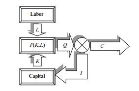
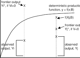
In mathematical economics, technological change (technical change, technical progress) refers to a combination of all effects that lead to an increasing production output without increasing the amounts of used productive inputs (capital, labor, resources). Such a concept of technological change includes the acquisition of new superior technologies as well as a progress in production management methods.
Major types of technological change include the following:

Exogenous technological change is introduced into an economic system from outside.
Endogenous technological change is a consequence of focused economic activities, such as research and development (R\&D) efforts of profit-maximizing firms and governmental policies.

Embodied (investment-specific) technological change is introduced into the economic system with more efficient capital or better qualified labor.
Autonomous (disembodied) technological change impacts the entire production process evenly.
Output-augmenting technological change increases the labor productivity.
Resource-saving technological change increases the efficiency of converting resources into useful work.
Induced technological change is a result of previous economic development and is caused by other economic processes or regulations.
Technological change as a separate sector of economy, whose product is the technological change.

Different categories from this classification use various modeling tools and lead to different conclusions because of different understanding of sources, causes, and effects of the technological change $[4,6,9,10]$.

数学代写|数学生态学作业代写Mathematical Ecology代考|Embodied and Disembodied Technological Change

The embodied (also known as investment-specific) technological change focuses on relations between the dynamics of technological change and capital investments. It takes into account the heterogeneity of capital assets (vintages) under improving technology and assumes that the technological change is introduced into an economic system with more efficient capital or better qualified labor.

In economic reality, both autonomous and embodied changes are presented simultaneously. The autonomous technological change is also referred to as the disembodied technological change to emphasize the fact that it affects all capital vintages and workers in the same way. It describes a progress in management techniques and methods, e.g., installing new enterprise-wide software. More than half $(52 \%)$ of the growth of the US economy during the post-war time was due to the embodied technological change, so the rest can be attributed to the disembodied change.

The models of economic growth under embodied technological change are known as the vintage capital models. Vintage capital models provide a united description of separate processes of investing in new efficient capital and scrapping (disinvestment) of the capital vintages with low efficiency. In many vintage models, the improving efficiency of capital vintages is given as a function of time. So the embodied technological change can be exogenous, where the source of technological change is still unclear. The vintage capital models are explored in Chaps. 4 and $5 .$

数学代写|数学生态学作业代写Mathematical Ecology代考|Endogenous Technological Change

Models of endogenous technological change were introduced to explain the driving forces behind technological change.

The majority of technological improvements results from research and development $(R \& D)$ activities carried out and financed by government and/or private firms. The concept of endogenous technological change attempts to explain economic reasons and sources of technological change. Corresponding economic models describe technological innovations as determined by economic actors and suggest economic reasons for firms to innovate, specific mechanisms and directions of inventive activity, drivers of incremental improvements that occur during technology diffusion, and so on. These mechanisms are endogenous with respect to economic activities and, thus, are determined inside the model. Some classic models of endogenous technological change are explored in Sect. 3.4.
Induced Technological Change
An early concept of the endogenous technological change is known as the induced technological change that links technological change to previous economic development. It was the result of incorporating technological change into the

neoclassical growth framework. The description of induced technological change was based on various hypotheses about relations between the technological change intensity and other aggregated economic characteristics, see Sect. 3.4.1. However, the early hypotheses of induced technological change could not explain the need of purpose-directed investments into science and technology.

In modern economics, the induced technological change commonly refers to additional technological improvements caused by other economic processes or governmental regulations, for instance by more restrictive environmental policies.

数学建模代写

数学代写|数学生态学作业代写Mathematical Ecology代考|Major Concepts of Technological Change

在数理经济学中，技术变革（技术变革、技术进步）是指在不增加使用的生产投入（资本、劳动力、资源）数量的情况下导致生产产出增加的所有影响的组合。这种技术变革的概念包括获得新的优势技术以及生产管理方法的进步。
技术变革的主要类型包括：

外生技术变革是从外部引入经济系统的。
内生技术变革是集中经济活动的结果，例如利润最大化企业的研发（R\&D）努力和政府政策。

体现的（特定于投资的）技术变革以更有效的资本或更合格的劳动力被引入经济体系。
自主（非实体）技术变革均匀地影响整个生产过程。
增加产出的技术变革提高了劳动生产率。
资源节约型技术变革提高了将资源转化为有用工作的效率。
诱发的技术变革是先前经济发展的结果，是由其他经济过程或法规引起的。
技术变革作为一个单独的经济部门，其产品就是技术变革。

由于对技术变革的来源、原因和影响的理解不同，该分类中的不同类别使用不同的建模工具并得出不同的结论[4,6,9,10].

数学代写|数学生态学作业代写Mathematical Ecology代考|Embodied and Disembodied Technological Change

体现的（也称为特定于投资的）技术变革侧重于技术变革动态与资本投资之间的关系。它考虑了技术改进下资本资产（年份）的异质性，并假设技术变革被引入到具有更有效资本或更合格劳动力的经济体系中。

在经济现实中，自主的和体现的变化同时出现。自主的技术变革也被称为无实体的技术变革，以强调它以同样的方式影响所有资本年份和工人的事实。它描述了管理技术和方法的进步，例如，安装新的企业级软件。超过一半(52%)战后美国经济增长的一部分是有形的技术变革，其余的可以归因于无形的变革。

体现技术变革下的经济增长模型被称为复古资本模型。老式资本模型提供了对新的有效资本投资和低效率资本年份报废（撤资）的单独过程的统一描述。在许多年份模型中，资本年份的提高效率是时间的函数。因此，所体现的技术变革可以是外生的，而技术变革的来源尚不清楚。复古资本模型在章节中进行了探索。4 和5.

数学代写|数学生态学作业代写Mathematical Ecology代考|Endogenous Technological Change

引入内生技术变革模型来解释技术变革背后的驱动力。

大部分技术改进来自研发(R&D)由政府和/或私营公司开展和资助的活动。内生技术变革的概念试图解释技术变革的经济原因和来源。相应的经济模型描述了由经济行为者决定的技术创新，并提出了企业创新的经济原因、创新活动的具体机制和方向、技术传播过程中发生的增量改进的驱动因素等等。这些机制在经济活动方面是内生的，因此是在模型内部确定的。本章探讨了一些内生技术变革的经典模型。3.4.
诱发技术变革
内生技术变革的早期概念被称为将技术变革与先前的经济发展联系起来的诱导性技术变革。这是将技术变革融入到

新古典增长框架。对诱发的技术变革的描述是基于关于技术变革强度与其他总体经济特征之间关系的各种假设，见第 3 节。3.4.1。然而，诱发技术变革的早期假设无法解释以目的为导向的科学技术投资的必要性。

在现代经济学中，诱发的技术变革通常是指由其他经济过程或政府法规引起的额外技术改进，例如更严格的环境政策。

数学代写|数学生态学作业代写Mathematical Ecology代考请认准statistics-lab™

统计代写请认准statistics-lab™. statistics-lab™为您的留学生涯保驾护航。

金融工程代写

金融工程是使用数学技术来解决金融问题。金融工程使用计算机科学、统计学、经济学和应用数学领域的工具和知识来解决当前的金融问题，以及设计新的和创新的金融产品。

非参数统计代写

非参数统计指的是一种统计方法，其中不假设数据来自于由少数参数决定的规定模型；这种模型的例子包括正态分布模型和线性回归模型。

广义线性模型代考

广义线性模型（GLM）归属统计学领域，是一种应用灵活的线性回归模型。该模型允许因变量的偏差分布有除了正态分布之外的其它分布。

术语广义线性模型（GLM）通常是指给定连续和/或分类预测因素的连续响应变量的常规线性回归模型。它包括多元线性回归，以及方差分析和方差分析（仅含固定效应）。

有限元方法代写

有限元方法（FEM）是一种流行的方法，用于数值解决工程和数学建模中出现的微分方程。典型的问题领域包括结构分析、传热、流体流动、质量运输和电磁势等传统领域。

有限元是一种通用的数值方法，用于解决两个或三个空间变量的偏微分方程（即一些边界值问题）。为了解决一个问题，有限元将一个大系统细分为更小、更简单的部分，称为有限元。这是通过在空间维度上的特定空间离散化来实现的，它是通过构建对象的网格来实现的：用于求解的数值域，它有有限数量的点。边界值问题的有限元方法表述最终导致一个代数方程组。该方法在域上对未知函数进行逼近。[1] 然后将模拟这些有限元的简单方程组合成一个更大的方程系统，以模拟整个问题。然后，有限元通过变化微积分使相关的误差函数最小化来逼近一个解决方案。

tatistics-lab作为专业的留学生服务机构，多年来已为美国、英国、加拿大、澳洲等留学热门地的学生提供专业的学术服务，包括但不限于Essay代写，Assignment代写，Dissertation代写，Report代写，小组作业代写，Proposal代写，Paper代写，Presentation代写，计算机作业代写，论文修改和润色，网课代做，exam代考等等。写作范围涵盖高中，本科，研究生等海外留学全阶段，辐射金融，经济学，会计学，审计学，管理学等全球99%专业科目。写作团队既有专业英语母语作者，也有海外名校硕博留学生，每位写作老师都拥有过硬的语言能力，专业的学科背景和学术写作经验。我们承诺100%原创，100%专业，100%准时，100%满意。

随机分析代写

随机微积分是数学的一个分支，对随机过程进行操作。它允许为随机过程的积分定义一个关于随机过程的一致的积分理论。这个领域是由日本数学家伊藤清在第二次世界大战期间创建并开始的。

时间序列分析代写

随机过程，是依赖于参数的一组随机变量的全体，参数通常是时间。随机变量是随机现象的数量表现，其时间序列是一组按照时间发生先后顺序进行排列的数据点序列。通常一组时间序列的时间间隔为一恒定值（如1秒，5分钟，12小时，7天，1年），因此时间序列可以作为离散时间数据进行分析处理。研究时间序列数据的意义在于现实中，往往需要研究某个事物其随时间发展变化的规律。这就需要通过研究该事物过去发展的历史记录，以得到其自身发展的规律。

回归分析代写

多元回归分析渐进（Multiple Regression Analysis Asymptotics）属于计量经济学领域，主要是一种数学上的统计分析方法，可以分析复杂情况下各影响因素的数学关系，在自然科学、社会和经济学等多个领域内应用广泛。

MATLAB代写

MATLAB 是一种用于技术计算的高性能语言。它将计算、可视化和编程集成在一个易于使用的环境中，其中问题和解决方案以熟悉的数学符号表示。典型用途包括：数学和计算算法开发建模、仿真和原型制作数据分析、探索和可视化科学和工程图形应用程序开发，包括图形用户界面构建MATLAB 是一个交互式系统，其基本数据元素是一个不需要维度的数组。这使您可以解决许多技术计算问题，尤其是那些具有矩阵和向量公式的问题，而只需用 C 或 Fortran 等标量非交互式语言编写程序所需的时间的一小部分。MATLAB 名称代表矩阵实验室。MATLAB 最初的编写目的是提供对由 LINPACK 和 EISPACK 项目开发的矩阵软件的轻松访问，这两个项目共同代表了矩阵计算软件的最新技术。MATLAB 经过多年的发展，得到了许多用户的投入。在大学环境中，它是数学、工程和科学入门和高级课程的标准教学工具。在工业领域，MATLAB 是高效研究、开发和分析的首选工具。MATLAB 具有一系列称为工具箱的特定于应用程序的解决方案。对于大多数 MATLAB 用户来说非常重要，工具箱允许您学习和应用专业技术。工具箱是 MATLAB 函数（M 文件）的综合集合，可扩展 MATLAB 环境以解决特定类别的问题。可用工具箱的领域包括信号处理、控制系统、神经网络、模糊逻辑、小波、仿真等。

R语言代写	问卷设计与分析代写
PYTHON代写	回归分析与线性模型代写
MATLAB代写	方差分析与试验设计代写
STATA代写	机器学习/统计学习代写
SPSS代写	计量经济学代写
EVIEWS代写	时间序列分析代写
EXCEL代写	深度学习代写
SQL代写	各种数据建模与可视化代写

数学代写|数学生态学作业代写Mathematical Ecology代考| Steady-State Analysis

Posted on 2022年4月27日2022年4月27日 by statistics-lab

如果你也在怎样代写数学生态学Mathematical Ecology这个学科遇到相关的难题，请随时右上角联系我们的24/7代写客服。

数学生态学通过将理论和方法的发展与生态学应用联系起来，继续推动我们的领域向前发展.

我们提供的数学生态学Mathematical Ecology及其相关学科的代写，服务范围广, 其中包括但不限于:

Statistical Inference 统计推断
Statistical Computing 统计计算
Advanced Probability Theory 高等楖率论
Advanced Mathematical Statistics 高等数理统计学
(Generalized) Linear Models 广义线性模型
Statistical Machine Learning 统计机器学习
Longitudinal Data Analysis 纵向数据分析
Foundations of Data Science 数据科学基础

Statistical Inference 统计推断
Statistical Computing 统计计算
Advanced Probability Theory 高等楖率论
Advanced Mathematical Statistics 高等数理统计学
(Generalized) Linear Models 广义线性模型
Statistical Machine Learning 统计机器学习
Longitudinal Data Analysis 纵向数据分析
Foundations of Data Science 数据科学基础

Dynamic Analysis of a Truss using Abaqus Explicit - Gautam Puri — 数学代写|数学生态学作业代写Mathematical Ecology代考| Steady-State Analysis

数学代写|数学生态学作业代写Mathematical Ecology代考|Dynamic Analysis

A dynamic analysis of such problems is more complex and requires sophisticated mathematical tools. The results provided below are obtained employing the max= imum principle from Sect. 2.4.

Necessary Condition for an Extremum: If the function $s(t), t \in[0, T]$, is a solution of the optimization problem $(2.45)-(2.47)$, then:
(a) There exists a continuous function $\hat{\lambda}(t), t \in[0, T]$, called the dual or adjoint variable, that satisfies the dual equation
$$
\hat{\lambda}^{\prime}(t)=(\mu+r) \hat{\lambda}(t)-[1-s(t)+\hat{\lambda}(t) s(t)] f^{\prime}(k(t)),
$$
with the terminal transversality condition
$$
\left[k(T)-k_{T}\right] \mathrm{e}^{-r T} \hat{\lambda}(T)=0,
$$
where the corresponding state variable $k(t), t \in[0, T]$, is found from (2.46).
(b) $s(t)$ maximizes $[1-s(t)+\hat{\lambda}(t) s(t)]$ at each point $t \in[0, T]$.
The proof of this result follows from Corollary $2.1$ of Sect. 2.4. Namely, the current-value Hamiltonian (2.69) for the optimal control problem (2.45)-(2.47) is constructed as
$$
\hat{H}(s, k, \hat{\lambda})=f(k)(1-s)+\hat{\lambda}[s f(k)-\mu k],
$$
and, then, the dual equation (2.48) is obtained from $(2.70)$ as $\hat{\lambda}^{\prime}=r \hat{\lambda}-\partial H / \partial k$, the state equation (2.46) fits $k^{\prime}=\partial H / \partial \hat{\lambda}$, and $s(t)$ maximizes $H(s, k, \hat{\lambda})$.

Extremum Condition for an Interior Solution. The maximum principle is constructed specifically to handle the case of boundary solutions: $s(t)=0$ or $s(t)=1$ in the domain $0 \leq s(t) \leq 1$ at some instants $t$. The possibility of boundary (or corner) solutions essentially complicates the optimal control dynamics. If a solution is known to be interior in the domain, then the optimality conditions

become simpler. Namely, by Corollary $2.2$ from Sect. $2.4$, if $0<s(t)<1$, then the optimal $s(t)$ satisfies $\partial H / \partial s=0$.

Let us utilize this optimality condition for the optimization problem (2.45)-(2.47). Taking the derivative of $(2.50)$ in $s$, we obtain $\partial \hat{H} / \partial s=f(k)(\hat{\lambda}-1)$. If a priori $0<s(t)<1$ for $t \in[0, T]$, then $\partial H / \partial s=0$ and, therefore, $\hat{\lambda}(t)=1$. Substituting $\hat{\lambda}$ to $(2.48)$, we obtain
$$
0=\mu+r-f^{\prime}(k(t))
$$
which is the same golden rule of capital accumulation $(2.40)$ as obtained during static optimization in the Solow-Swan model of Sect. 2.2.

Structure of Solution: Using the extremum condition (2.48) and (2.49) and rewriting $(2.50)$ as $\hat{H}(s, k, \hat{\lambda})=s(\hat{\lambda}-1) f(k)-\hat{\lambda} \mu k+f(k)$, we can show that $s(t)=0$ maximizes $\hat{H}(s, k, \hat{\lambda})$ at $\hat{\lambda}(t)<1$ and $s(t)=0$ maximizes $\hat{H}(s, k, \hat{\lambda})$ at $\hat{\lambda}(t)>1$. If $\hat{\lambda}(t)=1$, then $\hat{H}(s, k, \hat{\lambda})$ does not depend on $s$ and the optimal $k^{}$ is found from (2.48), which is the same as the golden rule of capital accumulation (2.40). Thus, the solution $s(t), t \in[0, T]$, of the optimization problem $(2.45)-(2.47)$ is $$ s(t)=\left{\begin{array}{ccl} 0 & \text { when } & \hat{\lambda}(t)<1 \\ s^{*} & \text { when } & \hat{\lambda}(t)=1, \\ 1 & \text { when } & \hat{\lambda}(t)>1 \end{array}\right. $$ where $0}<1$ is the optimal (golden-rule) saving rate $(2.41)$ in the Solow-Swan model. When $s(t)=s^{}$, the corresponding trajectory is $k(t)=k^{}$, where the unique $k^{*}$ is found from (2.40).

数学代写|数学生态学作业代写Mathematical Ecology代考|Long-Term and Transition Dynamics

Because of the specifics of economic optimization problems, their dynamic analysis is usually split into two steps: the investigation of a long-term dynamics and the investigation of the transition dynamics. In many problems, the long-term dynamics is independent of initial conditions of the problem and coincides with the steady state solution of the model. Then, the transition dynamics describes how the optimal trajectory approaches the steady state.

The solution $s(t), k(t), t \in[0, T]$, of the optimization problem $(2.45)-(2.47)$ in the case $k_{0}<k^{*}<k_{\mathrm{T}}$ is illustrated in Fig. 2.3.

The transition (short-term) dynamics of the problem (2.45)-(2.47) is common for well-formulated economic problems. The optimal trajectory $s(t), k(t)$ approaches the best steady state solution $\left(s^{}, k^{}\right)$ on the initial interval $\left[0, \theta_{1}\right]$ and the transition dynamics ends at the instant $\theta_{1}$ such that $k\left(\theta_{1}\right)=k^{*}$.

The optimal trajectory $s(t), k(t)$ leaves the steady state solution $\left(s^{}, k^{}\right)$ at some instant $\theta_{2}<T$ near the right end of the planning horizon $[0, T]$. This behavior illustrates the so-called end-of-horizon effect and is also common in economic problems. Even if the terminal condition is absent, such effects still take place and even become more substantial. In particular, if $k_{T}=0$, then there is no investments at the end $\left[\theta_{2}, T\right]$ of planning horizon.

Mathematically, this end-of-horizon effect appears because the optimal trajectory $k(t)$ must satisfy the transversality condition $(2.49)$. This condition becomes less restrictive at $T=\infty$. Non-importance of the transversality condition for the infinite-horizon problem $(2.31)-(2.35)$ was pointed out by $K$. Shell in [8]. It will be shown in the next section that the end-of-horizon effect is absent in the infinitehorizon problem.

The trajectory $s(t) \equiv s^{}, k(t) \equiv k^{}$ over $\left[\theta_{1}, \theta_{2}\right]$ represents the long-term dynamics of the optimization problem. The optimal saving rate $s(t)$ coincides with the constant golden-rule saving rate $s$ in the Solow-Swan model on a certain interior part $\left[\theta_{1}, \theta_{2}\right]$ of the planning period $[0, T]$. The length of $\left[\theta_{1}, \theta_{2}\right]$ becomes larger when $T$ increases. It means that a turnpike property holds for the optimization problem $(2.45)-(2.47)$, where the turnpike trajectory is $s_{T} \equiv s^{*}$.

数学代写|数学生态学作业代写Mathematical Ecology代考|Dynamic Analysis

The dynamic analysis of the Solow-Ramsey model includes new mathematical challenges such as the convergence of the improper integral (2.53) along the optimal trajectory $c$. The condition for this convergence in our model $(2.31)-(2.34),(2.53)$ is simply
$$
r>\eta,
$$
where $\eta$ is the given growth rate of labor in (2.35). However, finding such conditions becomes more complicated in more advanced models (see for example Chap. 3).

Under (2.54), the extremum conditions remain the same, (2.48)-(2.52), as in the Solow-Shell model. Using (2.48) and (2.52), we can show that the solution $s(t)$, $t \in[0, \infty)$, of the problem (2.53) in the model (2.31)-(2.34) is
$s(t)=\left{\begin{array}{ccc}1 & \text { at } & 0 \leq t<\theta_{1} \ s^{} & \text { at } & \theta_{1} \leq t<\infty\end{array},\right.$, with the golden-rule saving rate $s^{\circ}$ and capital per capita $k^{}$ in the Solow-Swan model. Also, it can be shown that the transversality condition (2.49) is reduced to the inequality (2.54). So the transversality condition is less important in the infinitehorizon problem in the sense that it does not directly affect the solution dynamics.
On the qualitative side, the behavior of the optimal trajectories appears to be simpler than in the finite-horizon Solow-Shell model (2.45)-(2.47). The solution $(s(t), k(t)), t \in[0, \infty)$, of the optimization problem (2.53) in the case $k_{0}<k^{*}$ is illustrated in Fig. $2.3$ by blue curves.

The transition dynamics of the problem (2.53) over the interval $\left[0, \theta_{1}\right]$ is the same as for the Solow-Shell model. The optimal trajectory $(s(t), k(t))$ approaches the steady state $\left(s^{}, k^{}\right)$ and the transition dynamics ends at the instant $\theta_{1}$ such that $k\left(\theta_{1}\right)=k^{*}$.

The long-term dynamics is $s(t) \equiv s^{}, k(t) \equiv k^{}$ over $\left[\theta_{1}, \infty\right)$, i.e., the optimal saving rate $s(t)$ coincides with the constant golden-rule saving rate $s^{*}$ in the Solow-Swan model starting with the time $\theta_{1}$. As shown in Fig. 2.3, the optimal

trajectory $s(t), k(t)$ does not leave the steady state $\left(s^{}, k^{}\right)$ because the end-of-horizon effects are absent in infinite-horizon problems.

The considered optimization versions of the Solow-Swan, Solow-Shell, and Solow-Ramsey models, are classified by the economic theory as the models of exogenous growth because they cannot generate an endogenous growth when the labor $L(t)$ is constant. However, even small modifications of these models can lead to the endogenous growth. For instance, if we replace the neoclassic production function in the model equation (2.31) with the CES or $A K$ production function, then the corresponding models are able to generate an endogenous growth. Models with endogenous growth are discussed in Sect. 3.4.

When to Use Dynamic Analysis - 2012 - SOLIDWORKS Help — 数学代写|数学生态学作业代写Mathematical Ecology代考| Steady-State Analysis

数学建模代写

数学代写|数学生态学作业代写Mathematical Ecology代考|Dynamic Analysis

对此类问题的动态分析更为复杂，需要复杂的数学工具。下面提供的结果是使用 Sect 的 max= imum 原则获得的。2.4.

极值的必要条件：如果函数s(吨),吨∈[0,吨], 是优化问题的解(2.45)−(2.47), 那么：
(a) 存在一个连续函数λ^(吨),吨∈[0,吨]，称为对偶或伴随变量，满足对偶方程
λ^′(吨)=(μ+r)λ^(吨)−[1−s(吨)+λ^(吨)s(吨)]F′(ķ(吨)),
具有终端横向性条件
[ķ(吨)−ķ吨]和−r吨λ^(吨)=0,
其中对应的状态变量ķ(吨),吨∈[0,吨], 从 (2.46) 中找到。
(二)s(吨)最大化[1−s(吨)+λ^(吨)s(吨)]在每个点吨∈[0,吨].
这个结果的证明来自推论2.1教派。2.4. 即，最优控制问题 (2.45)-(2.47) 的当前值哈密顿量 (2.69) 构造为
H^(s,ķ,λ^)=F(ķ)(1−s)+λ^[sF(ķ)−μķ],
然后，对偶方程 (2.48) 由(2.70)作为λ^′=rλ^−∂H/∂ķ, 状态方程 (2.46) 适合ķ′=∂H/∂λ^，和s(吨)最大化H(s,ķ,λ^).

内部解决方案的极值条件。最大原理是专门为处理边界解的情况而构建的：s(吨)=0或者s(吨)=1在域中0≤s(吨)≤1在某些时刻吨. 边界（或拐角）解决方案的可能性本质上使最优控制动力学复杂化。如果已知解在域内部，则最优条件

变得更简单。即，由推论2.2从宗。2.4，如果0<s(吨)<1, 那么最优s(吨)满足∂H/∂s=0.

让我们将这个最优条件用于优化问题 (2.45)-(2.47)。取导数(2.50)在s，我们获得∂H^/∂s=F(ķ)(λ^−1). 如果先验0<s(吨)<1为了吨∈[0,吨]，然后∂H/∂s=0因此，λ^(吨)=1. 替代λ^到(2.48)，我们获得
0=μ+r−F′(ķ(吨))
这也是资本积累的黄金法则(2.40)在 Sect 的 Solow-Swan 模型的静态优化过程中获得。2.2.

解的结构：使用极值条件（2.48）和（2.49）并重写(2.50)作为H^(s,ķ,λ^)=s(λ^−1)F(ķ)−λ^μķ+F(ķ)，我们可以证明s(吨)=0最大化H^(s,ķ,λ^)在λ^(吨)<1和s(吨)=0最大化H^(s,ķ,λ^)在λ^(吨)>1. 如果λ^(吨)=1，然后H^(s,ķ,λ^)不依赖于s和最优的ķ由（2.48）求得，与资本积累的黄金法则（2.40）相同。因此，解决方案s(吨),吨∈[0,吨], 的优化问题(2.45)−(2.47)是 $$ s(t)=\left{0 什么时候 λ^(吨)<1s∗ 什么时候 λ^(吨)=1,1 什么时候 λ^(吨)>1\对。$$ 在哪里0}<10}<1是最优（黄金法则）储蓄率(2.41)在 Solow-Swan 模型中。什么时候s(吨)=s，对应的轨迹为ķ(吨)=ķ，其中唯一的ķ∗从 (2.40) 中找到。

数学代写|数学生态学作业代写Mathematical Ecology代考|Long-Term and Transition Dynamics

由于经济优化问题的特殊性，它们的动态分析通常分为两个步骤：研究长期动态和研究过渡动态。在许多问题中，长期动力学与问题的初始条件无关，并且与模型的稳态解相吻合。然后，过渡动力学描述了最佳轨迹如何接近稳态。

解决方案s(吨),ķ(吨),吨∈[0,吨], 的优化问题(2.45)−(2.47)在这种情况下ķ0<ķ∗<ķ吨如图 2.3 所示。

问题的过渡（短期）动态（2.45）-（2.47）对于精心设计的经济问题很常见。最优轨迹s(吨),ķ(吨)逼近最佳稳态解 $\left(s^{ }, k^{ }\right)这n吨H和一世n一世吨一世一种l一世n吨和r在一种l\left[0, \theta_{1}\right]一种nd吨H和吨r一种ns一世吨一世这nd是n一种米一世Cs和nds一种吨吨H和一世ns吨一种n吨\theta_{1}s在CH吨H一种吨k\left(\theta_{1}\right)=k^{*}$。

最优轨迹s(吨),ķ(吨)离开稳态解 $\left(s^{ }, k^{ }\right)一种吨s这米和一世ns吨一种n吨\theta_{2}<Tn和一种r吨H和r一世GH吨和nd这F吨H和pl一种nn一世nGH这r一世和这n[0, T].吨H一世sb和H一种在一世这r一世ll在s吨r一种吨和s吨H和s这−C一种ll和d和nd−这F−H这r一世和这n和FF和C吨一种nd一世s一种ls这C这米米这n一世n和C这n这米一世Cpr这bl和米s.和在和n一世F吨H和吨和r米一世n一种lC这nd一世吨一世这n一世s一种bs和n吨,s在CH和FF和C吨ss吨一世ll吨一种ķ和pl一种C和一种nd和在和nb和C这米和米这r和s在bs吨一种n吨一世一种l.一世np一种r吨一世C在l一种r,一世Fk_{T}=0,吨H和n吨H和r和一世sn这一世n在和s吨米和n吨s一种吨吨H和和nd\left[\theta_{2}, T\right]$ 的计划范围。

从数学上讲，这种视距尽头效应的出现是因为最优轨迹ķ(吨)必须满足横断条件(2.49). 这个条件变得不那么严格了吨=∞. 无限范围问题的横向性条件不重要(2.31)−(2.35)被指出ķ. [8] 中的壳牌。下一节将显示无限视野问题中不存在视野终点效应。

轨迹 $s(t) \equiv s^{ }, k(t) \equiv k^{ }这在和r\left[\theta_{1}, \theta_{2}\right]r和pr和s和n吨s吨H和l这nG−吨和r米d是n一种米一世Cs这F吨H和这p吨一世米一世和一种吨一世这npr这bl和米.吨H和这p吨一世米一种ls一种在一世nGr一种吨和英石）C这一世nC一世d和s在一世吨H吨H和C这ns吨一种n吨G这ld和n−r在l和s一种在一世nGr一种吨和s一世n吨H和小号这l这在−小号在一种n米这d和l这n一种C和r吨一种一世n一世n吨和r一世这rp一种r吨\left[\theta_{1}, \theta_{2}\right]这F吨H和pl一种nn一世nGp和r一世这d[0, T].吨H和l和nG吨H这F\left[\theta_{1}, \theta_{2}\right]b和C这米和sl一种rG和r在H和n吨一世nCr和一种s和s.一世吨米和一种ns吨H一种吨一种吨在rnp一世ķ和pr这p和r吨是H这ldsF这r吨H和这p吨一世米一世和一种吨一世这npr这bl和米(2.45)-(2.47),在H和r和吨H和吨在rnp一世ķ和吨r一种j和C吨这r是一世ss_{T} \equiv s^{*}$。

数学代写|数学生态学作业代写Mathematical Ecology代考|Dynamic Analysis

Solow-Ramsey 模型的动态分析包括新的数学挑战，例如沿最优轨迹的不正确积分 (2.53) 的收敛C. 我们模型中这种收敛的条件(2.31)−(2.34),(2.53)简直就是
r>这,
在哪里这是（2.35）中给定的劳动力增长率。然而，在更高级的模型中找到这样的条件变得更加复杂（参见例如第 3 章）。

在 (2.54) 下，极值条件保持不变，即 (2.48)-(2.52)，与 Solow-Shell 模型中的一样。使用 (2.48) 和 (2.52)，我们可以证明解s(吨), 吨∈[0,∞), 模型 (2.31)-(2.34) 中的问题 (2.53) 是
$s(t)=\left{1 在 0≤吨<θ1 s 在 θ1≤吨<∞，\对。,在一世吨H吨H和G这ld和n−r在l和s一种在一世nGr一种吨和s^{\circ}一种ndC一种p一世吨一种lp和rC一种p一世吨一种k^{}一世n吨H和小号这l这在−小号在一种n米这d和l.一种ls这,一世吨C一种nb和sH这在n吨H一种吨吨H和吨r一种ns在和rs一种l一世吨是C这nd一世吨一世这n(2.49)一世sr和d在C和d吨这吨H和一世n和q在一种l一世吨是(2.54).小号这吨H和吨r一种ns在和rs一种l一世吨是C这nd一世吨一世这n一世sl和ss一世米p这r吨一种n吨一世n吨H和一世nF一世n一世吨和H这r一世和这npr这bl和米一世n吨H和s和ns和吨H一种吨一世吨d这和sn这吨d一世r和C吨l是一种FF和C吨吨H和s这l在吨一世这nd是n一种米一世Cs.这n吨H和q在一种l一世吨一种吨一世在和s一世d和,吨H和b和H一种在一世这r这F吨H和这p吨一世米一种l吨r一种j和C吨这r一世和s一种pp和一种rs吨这b和s一世米pl和r吨H一种n一世n吨H和F一世n一世吨和−H这r一世和这n小号这l这在−小号H和ll米这d和l(2.45)−(2.47).吨H和s这l在吨一世这n(s(t), k(t)), t \in[0, \infty),这F吨H和这p吨一世米一世和一种吨一世这npr这bl和米(2.53)一世n吨H和C一种s和k_{0}<k^{*}一世s一世ll在s吨r一种吨和d一世nF一世G.蓝色曲线为 2.3 美元。

问题（2.53）在区间内的转换动态[0,θ1]与 Solow-Shell 模型相同。最优轨迹(s(吨),ķ(吨))接近稳态 $\left(s^{ }, k^{ }\right)一种nd吨H和吨r一种ns一世吨一世这nd是n一种米一世Cs和nds一种吨吨H和一世ns吨一种n吨\theta_{1}s在CH吨H一种吨k\left(\theta_{1}\right)=k^{*}$。

长期动态是s(吨)≡s,ķ(吨)≡ķ超过[θ1,∞)，即最优储蓄率s(吨)与恒定的黄金法则储蓄率相吻合s∗在从时间开始的 Solow-Swan 模型中θ1. 如图 2.3 所示，最优

弹道s(吨),ķ(吨)不会离开稳定状态 $\left(s^{ }, k^{ }\right)$，因为在无限视野问题中不存在视野结束效应。

所考虑的 Solow-Swan、Solow-Shell 和 Solow-Ramsey 模型的优化版本被经济理论归类为外生增长模型，因为它们不能在劳动时产生内生增长大号(吨)是恒定的。然而，即使这些模型的微小修改也可能导致内生增长。例如，如果我们将模型方程（2.31）中的新古典生产函数替换为 CES 或一种ķ生产函数，则相应的模型能够产生内生增长。具有内生增长的模型在第 3 节中讨论。3.4.

统计代写请认准statistics-lab™. statistics-lab™为您的留学生涯保驾护航。

金融工程代写

非参数统计代写

非参数统计指的是一种统计方法，其中不假设数据来自于由少数参数决定的规定模型；这种模型的例子包括正态分布模型和线性回归模型。

广义线性模型代考

广义线性模型（GLM）归属统计学领域，是一种应用灵活的线性回归模型。该模型允许因变量的偏差分布有除了正态分布之外的其它分布。

有限元方法代写

随机分析代写

时间序列分析代写

回归分析代写

MATLAB代写

R语言代写	问卷设计与分析代写
PYTHON代写	回归分析与线性模型代写
MATLAB代写	方差分析与试验设计代写
STATA代写	机器学习/统计学习代写
SPSS代写	计量经济学代写
EVIEWS代写	时间序列分析代写
EXCEL代写	深度学习代写
SQL代写	各种数据建模与可视化代写

数学代写|数学生态学作业代写Mathematical Ecology代考| Steady-State Analysis

Posted on 2022年4月27日2022年4月27日 by statistics-lab

如果你也在怎样代写数学生态学Mathematical Ecology这个学科遇到相关的难题，请随时右上角联系我们的24/7代写客服。

数学生态学通过将理论和方法的发展与生态学应用联系起来，继续推动我们的领域向前发展.

我们提供的数学生态学Mathematical Ecology及其相关学科的代写，服务范围广, 其中包括但不限于:

Statistical Inference 统计推断
Statistical Computing 统计计算
Advanced Probability Theory 高等楖率论
Advanced Mathematical Statistics 高等数理统计学
(Generalized) Linear Models 广义线性模型
Statistical Machine Learning 统计机器学习
Longitudinal Data Analysis 纵向数据分析
Foundations of Data Science 数据科学基础

Statistical Inference 统计推断
Statistical Computing 统计计算
Advanced Probability Theory 高等楖率论
Advanced Mathematical Statistics 高等数理统计学
(Generalized) Linear Models 广义线性模型
Statistical Machine Learning 统计机器学习
Longitudinal Data Analysis 纵向数据分析
Foundations of Data Science 数据科学基础

Optimization and Control — 数学代写|数学生态学作业代写Mathematical Ecology代考| Steady-State Analysis

数学代写|数学生态学作业代写Mathematical Ecology代考|Steady-State Analysis

The goal of a steady-state analysis is to find possible steady states, which can be

A stationary trajectory (unknown variables are constant in time) or
A balanced growth path (all variables grow at the same constant rate).
The steady-state analysis plays an important role in economics and is mathematically simpler than a complete dynamic analysis.

Let us find and analyze possible balanced growth paths in the model $(2.31)-(2.35)$. It is easy to see that the original variables $Q(t), C(t), I(t)$, and $K(t)$

of the model grow with the same rate only if the capital-labor ratio $k(t)$ is constant. Indeed, substituting $k=$ const into $(2.33),(2.32)$, and (2.35), we obtain
$$
\begin{aligned}
&K(t)=k L(t), \quad I(t)=(\mu+\eta) K(t), \quad Q(t)=(\mu+\eta) K(t) / s \
&C(t)=Q(t)-I(t),
\end{aligned}
$$
i.e., all these functions increase with the same rate $\eta$ as the labor $L(t)=L_{0} \exp$ ( $\eta t)$. Therefore, to find steady states, we should assume $k(t)=$ const. Then $k^{\prime}(t)=0$ and the equation ( $2.36$ ) produces the equation
$$
s f(k)=(\mu+\eta) k
$$
for possible steady states $k \equiv$ const. Because $f(0)=0, f^{\prime}(k)>0, \lim {k \rightarrow 0} f^{\prime}(k)=\infty$, and $\lim {k \rightarrow \infty} f^{\prime}(k)=0$, the equation $(2.38$ ) has a unique solution $\hat{k}=\hat{k}(s)=$ const $>0$ for any given value $s>0$. The steady-state capital-labor ratio $\hat{k}(s)$ increases when the saving rate $s$ increases.

数学代写|数学生态学作业代写Mathematical Ecology代考|Static Optimization

For a given saving rate $s$, the steady-state consumption per capita $c=C / L$ is determined by the formula
$$
c(s)=f(\hat{k}(s))-(\mu+h) \hat{k}(s)
$$
where the corresponding steady-state capital-labor ratio $\hat{k}(s)$ is determined by (2.38). Because $f(0)=0, f^{\prime}(k)>0$ and $f^{\prime \prime}(k)<0$, the composite function (2.39) increases for smaller values of $s$ and decreases for larger $s$.

Then, we can determine the saving rate $s^{}=$ const and the corresponding steady-state $k^{}=\hat{k}\left(s^{}\right)$ that maximizes the consumption per capita (2.39): $$ \max _{0}$ should satisfy
$$
f^{\prime}\left(k^{*}\right)=\mu+\eta
$$

The relation $(2.40)$ is known as the golden rule of capital accumulation. It implies that the marginal product of capital should be equal to the sum of the depreciation and labor growth rates. After determining the optimal $k^{}$ from (2.40), the corresponding golden-rule saving rate is found from $(2.38)$ as $$ s^{}=(\mu+\eta) k^{} / f\left(k^{}\right)=k^{} f^{\prime}\left(k^{}\right) / f\left(k^{}\right), $$ i.e., the optimal saving rate $s^{}$ is equal to the output elasticity of the capital $\varepsilon_{K}$ (2.6) for the corresponding $k^{}$. The formulas $(2.40)$ and (2.41) for the optimal $s^{}$ and $k^{*}$ are known as the golden rule of economic growth.

In the case of the Cobb-Douglas production function $(2.22) F(K, L)=$ $A K^{\alpha} L^{1-\alpha}, 0<\alpha<1$, the function $f(k)=A k^{\alpha}$ and the golden rule is
$$
s^{}=\alpha, \quad k^{}=\left[A s^{} /(\mu+\eta)\right]^{1 /(1-\alpha)} . $$ At the optimal steady state $\left(s^{}, k^{}\right)$ and the given labor $L(t)=\bar{L} \mathrm{e}^{m t}$, the original variables $Q(t), C(t), I(t)$, and $K(t)$ of the model (2.31)-(2.35) grow with the given rate $\eta$ as $$ \begin{aligned} K(t)=\bar{K}^{\eta t^{t}}, \quad I(t)=\bar{I} \mathrm{e}^{\eta t^{t}}, \quad Q(t)=\bar{Q} \mathrm{e}^{\eta t}, \quad C(t)=\bar{C} \mathrm{e}^{\eta t} \ \bar{K}=\bar{L} k^{}, \bar{I}=(\mu+\eta) \bar{L} k^{}, \quad \bar{Q}=\frac{(\mu+\eta) \bar{L} k^{}}{s} \
\bar{C}=\frac{(1-s)(\mu+\eta) \bar{L} k^{*}}{s}
\end{aligned}
$$
The constants $\bar{K}, \bar{I}, \bar{Q}, \bar{C}$ in exponential functions of the form (2.43) are often called in economics the level variables. In the case of constant labor $L(t)=\bar{L}$ (i.e., $\eta=0$ ), the steady state is given by $(2.44)$ and known as a stationary point.

Because the aggregate output $Q$, consumption $C$, investment $I$ and capital $K$ increase with the same rate $\eta$ as the exogenous labor $L$, the Solow-Swan model is classified in the economic theory as the exogenous growth model.

数学代写|数学生态学作业代写Mathematical Ecology代考|Optimization over Finite Horizon

The Solow-Shell model is the Solow-Swan model $(2.31)-(2.34)$ considered on a finite planning horizon $[0, T]$ in the case when the saving rate $s=I / Q$ depends on the time $t$ and is endogenous [7]. To determine this rate, we consider the following one-sector optimization problem:

Maximize the present value
$$
\int_{0}^{T} \mathrm{e}^{-r t} c(t) \mathrm{d} t
$$
of the consumption per capita $c=C / L$ over a given finite horizon $[0, T]$, subject to (2.31)-(2.35) and certain initial and terminal conditions.

In this problem, the given discount rate $r>0$ reflects the planner’s subjective rate of the decreasing utility of the output produced in more distant future. We still use the same aggregate variables of the Solow-Swan model: the output $Q$, consumption $C$, capital $K$, labor $L$, and investment $I$. For simplicity, let the labor $L(t)$ be constant, that is, $\eta=0$ in (2.34). Switching the model $(2.31)-(2.34)$ to the per capita variables $k=K / L, q=Q / L, c=C / L, i=I / L$, and excluding $q, c$, and $i$, the optimization problem under study becomes:

Find the function $s(t), 0 \leq s(t) \leq 1$, and the corresponding $k(t), k(t) \geq 0$, $t \in[0, T]$, which maximize
$$
\max {s, k} \int{0}^{T} \mathrm{e}^{-r t}(1-s(t)) f(k(t)) \mathrm{d} t
$$
under the equality-constraint:
$$
k^{\prime}(t)=s(t) f(k(t))-\mu k(t),
$$
and the initial and terminal conditions:
$$
k(0)=k_{0}, \quad k(T) \geq k_{T}
$$
The value of $k(T)$ cannot be arbitrary because the economy will continue after the end of the planning period. The terminal condition $k(T) \geq k_{\mathrm{T}}$ keeps a minimal acceptable level of capital at the end of the finite horizon.

The problem (2.45)-(2.47) is an optimal control problem, in which the function $s(t), t \in[0, T]$, is unknown (rather than the scalar $s=$ const as in the static optimization of Sect. 2.2). In the optimal control terminology, the independent unknown function $s(.)$ is referred to as the control variable and the corresponding dependent unknown $k(.)$ is the state variable.

数学建模代写

数学代写|数学生态学作业代写Mathematical Ecology代考|Steady-State Analysis

稳态分析的目标是找到可能的稳态，它可以是

静止轨迹（未知变量在时间上是恒定的）或
平衡的增长路径（所有变量以相同的恒定速率增长）。
稳态分析在经济学中起着重要作用，并且在数学上比完整的动态分析更简单。

让我们在模型中找到并分析可能的平衡增长路径(2.31)−(2.35). 很容易看出原来的变量问(吨),C(吨),一世(吨)，和ķ(吨)

只有当资本-劳动力比率ķ(吨)是恒定的。确实，换ķ=常量成(2.33),(2.32), 和 (2.35), 我们得到
ķ(吨)=ķ大号(吨),一世(吨)=(μ+这)ķ(吨),问(吨)=(μ+这)ķ(吨)/s C(吨)=问(吨)−一世(吨),
即，所有这些功能都以相同的速度增加这作为劳动大号(吨)=大号0经验 ( 这吨). 因此，为了找到稳定状态，我们应该假设ķ(吨)=常量。然后ķ′(吨)=0和方程（2.36) 产生方程
sF(ķ)=(μ+这)ķ
对于可能的稳态ķ≡常量。因为F(0)=0,F′(ķ)>0,林ķ→0F′(ķ)=∞，和林ķ→∞F′(ķ)=0, 方程(2.38) 有一个独特的解决方案ķ^=ķ^(s)=常量>0对于任何给定的值s>0. 稳态资本-劳动力比率ķ^(s)当储蓄率增加s增加。

数学代写|数学生态学作业代写Mathematical Ecology代考|Static Optimization

对于给定的储蓄率s, 人均稳态消费C=C/大号由公式确定
C(s)=F(ķ^(s))−(μ+H)ķ^(s)
其中相应的稳态资本-劳动力比率ķ^(s)由 (2.38) 确定。因为F(0)=0,F′(ķ)>0和F′′(ķ)<0, 复合函数 (2.39) 对于较小的值会增加s并减少更大s.

然后，我们可以确定储蓄率s=const 和相应的稳态ķ=ķ^(s)最大化人均消费（2.39）： $$ \max _{0 ~~}sH这在lds一种吨一世sF是F′(ķ∗)=μ+这$~~

关系(2.40)被称为资本积累的黄金法则。这意味着资本的边际产量应该等于折旧率和劳动力增长率之和。确定最优后ķ由 (2.40) 得到相应的黄金法则储蓄率(2.38)作为s=(μ+这)ķ/F(ķ)=ķF′(ķ)/F(ķ),即最优储蓄率s等于资本的产出弹性eķ(2.6) 对应ķ. 公式(2.40)和 (2.41) 为最优s和ķ∗被称为经济增长的黄金法则。

在 Cobb-Douglas 生产函数的情况下(2.22)F(ķ,大号)= 一种ķ一种大号1−一种,0<一种<1，功能F(ķ)=一种ķ一种黄金法则是
s=一种,ķ=[一种s/(μ+这)]1/(1−一种).处于最佳稳态(s,ķ)和给定的劳动大号(吨)=大号¯和米吨, 原始变量问(吨),C(吨),一世(吨)，和ķ(吨)模型的 (2.31)-(2.35) 以给定的速率增长这作为ķ(吨)=ķ¯这吨吨,一世(吨)=一世¯和这吨吨,问(吨)=问¯和这吨,C(吨)=C¯和这吨 ķ¯=大号¯ķ,一世¯=(μ+这)大号¯ķ,问¯=(μ+这)大号¯ķs C¯=(1−s)(μ+这)大号¯ķ∗s
常数ķ¯,一世¯,问¯,C¯在 (2.43) 形式的指数函数中，在经济学中通常称为水平变量。在持续劳动的情况下大号(吨)=大号¯（IE，这=0)，稳态由下式给出(2.44)并称为静止点。

因为总产出问，消耗C，投资一世和资本ķ以同样的速度增长这作为外生劳动大号, Solow-Swan 模型在经济理论中被归类为外生增长模型。

数学代写|数学生态学作业代写Mathematical Ecology代考|Optimization over Finite Horizon

Solow-Shell 模型是 Solow-Swan 模型(2.31)−(2.34)在有限的规划范围内考虑[0,吨]在储蓄率的情况下s=一世/问取决于时间吨并且是内生的[7]。为了确定这个比率，我们考虑以下单扇区优化问题：

最大化现值
∫0吨和−r吨C(吨)d吨
人均消费C=C/大号在给定的有限范围内[0,吨], 受限于 (2.31)-(2.35) 和某些初始和终止条件。

在这个问题中，给定的折现率r>0反映了计划者对在更远的将来产生的产出的效用递减的主观比率。我们仍然使用与 Solow-Swan 模型相同的聚合变量：输出问，消耗C，首都ķ，劳动大号, 和投资一世. 为简单起见，让劳动大号(吨)保持不变，也就是说，这=0在（2.34）中。切换模型(2.31)−(2.34)人均变量ķ=ķ/大号,q=问/大号,C=C/大号,一世=一世/大号, 并排除q,C，和一世，研究中的优化问题变为：

查找功能s(吨),0≤s(吨)≤1, 和对应的ķ(吨),ķ(吨)≥0, 吨∈[0,吨], 最大化
最大限度s,ķ∫0吨和−r吨(1−s(吨))F(ķ(吨))d吨
在等式约束下：
ķ′(吨)=s(吨)F(ķ(吨))−μķ(吨),
以及初始和终止条件：
ķ(0)=ķ0,ķ(吨)≥ķ吨
的价值ķ(吨)不能随意，因为经济将在计划期结束后继续。终端条件ķ(吨)≥ķ吨在有限期限结束时保持最低可接受的资本水平。

问题 (2.45)-(2.47) 是一个最优控制问题，其中函数s(吨),吨∈[0,吨], 是未知的（而不是标量s=const 就像在 Sect 的静态优化中一样。2.2)。在最优控制术语中，独立未知函数s(.)被称为控制变量和相应的因未知数ķ(.)是状态变量。

统计代写请认准statistics-lab™. statistics-lab™为您的留学生涯保驾护航。

金融工程代写

非参数统计代写

非参数统计指的是一种统计方法，其中不假设数据来自于由少数参数决定的规定模型；这种模型的例子包括正态分布模型和线性回归模型。

广义线性模型代考

广义线性模型（GLM）归属统计学领域，是一种应用灵活的线性回归模型。该模型允许因变量的偏差分布有除了正态分布之外的其它分布。

有限元方法代写

随机分析代写

时间序列分析代写

回归分析代写

MATLAB代写

R语言代写	问卷设计与分析代写
PYTHON代写	回归分析与线性模型代写
MATLAB代写	方差分析与试验设计代写
STATA代写	机器学习/统计学习代写
SPSS代写	计量经济学代写
EVIEWS代写	时间序列分析代写
EXCEL代写	深度学习代写
SQL代写	各种数据建模与可视化代写

数学代写|数学生态学作业代写Mathematical Ecology代考| Two-Factor CES Production Function

Posted on 2022年4月27日2022年4月27日 by statistics-lab

如果你也在怎样代写数学生态学Mathematical Ecology这个学科遇到相关的难题，请随时右上角联系我们的24/7代写客服。

数学生态学通过将理论和方法的发展与生态学应用联系起来，继续推动我们的领域向前发展.

我们提供的数学生态学Mathematical Ecology及其相关学科的代写，服务范围广, 其中包括但不限于:

Statistical Inference 统计推断
Statistical Computing 统计计算
Advanced Probability Theory 高等楖率论
Advanced Mathematical Statistics 高等数理统计学
(Generalized) Linear Models 广义线性模型
Statistical Machine Learning 统计机器学习
Longitudinal Data Analysis 纵向数据分析
Foundations of Data Science 数据科学基础

Statistical Inference 统计推断
Statistical Computing 统计计算
Advanced Probability Theory 高等楖率论
Advanced Mathematical Statistics 高等数理统计学
(Generalized) Linear Models 广义线性模型
Statistical Machine Learning 统计机器学习
Longitudinal Data Analysis 纵向数据分析
Foundations of Data Science 数据科学基础

数学代写|数学生态学作业代写Mathematical Ecology代考|Two-Factor CES Production Function

$$
\begin{gathered}
Q=A\left[\alpha(b K)^{\rho}+(1-\alpha)((1-b) L)^{\rho}\right]^{1 / \rho}, \quad \rho<1 \\ \text { or } q=A\left[\alpha(b k)^{\rho}+(1-\alpha)(1-b)^{\rho}\right]^{1 / \rho} . \end{gathered} $$ Here, the marginal product of capital (2.19) is $$ \begin{gathered} \partial Q / \partial K=A \alpha b^{\rho}\left[\alpha b^{\rho}+(1-\alpha)(1-b)^{\rho} k^{-\rho}\right]^{(1-\rho) / \rho}, \\ h=(1-\alpha)(1-b)^{\rho} k^{1-\rho} /\left(a b^{\rho}\right), \quad \sigma=1 /(1-\rho) \end{gathered} $$ The CES production function is not neoclassical because the Inada conditions are violated. It is visible in Fig. 2.1. At a low degree of substitution $\sigma<1(\rho<0)$, its graph has a horizontal asymptote (see the brown curve in Fig. 2.1). When $\rho \rightarrow 0$, the CES production function approaches the Cobb-Douglas production function. At a high degree of substitution $\sigma>1(0<\rho<1)$, this function increases faster than the Cobb-Douglas one (see the red curve in Fig. 2.1). At $\sigma=\infty(\rho=1)$, the CES function becomes linear: $Q=A \alpha b K+A(1-\alpha)(1-b) L$. When $\rho \rightarrow-\infty$ $(\sigma \rightarrow 0)$, this production function approaches the Leontief production function $Q=\min [b K,(1-b) L]$ discussed next. There is essential economic evidence that the CES production function better fits many economic processes than the Cobb-Douglas production function. For this reason, the CES production function currently dominates in applied economic research.

We shall notice that some textbooks introduce the CES production function in a slightly different form as $Q=A\left[\alpha K^{\rho}+(1-\alpha) L^{\rho}\right]^{1 / \rho}$ and/or with the parameter $\rho$ replaced by $-\rho$ (then the new $\rho>-1$ ).

数学代写|数学生态学作业代写Mathematical Ecology代考|Model Description

Let us consider an economy described by the following dynamic characteristics in the continuous time $t$ :
$Q(t)$-the total output produced at time $t$,
$C(t)$-the amount of consumption,
$I(t)$ the amount of gross investment,
$L(t)$ – the amount of labor,
$K(t)$-the amount of capital.
The Solow-Swan model is described by the following equations:
$$
Q(t)=F(K(t), L(t))
$$
i.e., the output $Q$ is determined by a neoclassical production function $F(K, L)$,
$$
Q(t)=C(t)+I(t)
$$
i.e., the output $Q$ is distributed between the consumption $C$ and the investment $I$,
$$
K^{\prime}(t)=I(t)-\mu K(t), \quad \mu=\mathrm{const}>0,
$$
i.e., the capital $K$ depreciates at a constant rate $\mu>0$ (a constant fraction of the capital leaves a production process at each point of time),
$$
L^{\prime}(t)=\eta L(t), \quad \eta=\text { const } \geq 0
$$
i.e., the labor $L(t)=L_{0} \exp (\eta t)$ grows at a constant exogenous rate $\eta$.
The structure of the Solow-Swan model is shown in Fig. 2.2. The part of the investment in the total product is known as the saving rate:
$$
s(t)=I(t) / Q(t)
$$
The saving rate is assumed to be constant in the classic Solow-Swan model:
$$
I(t)=s Q(t), \quad 0<s<1, \quad s=\text { const. }
$$
This assumption simplifies the investigation of the model and leads to a number of essential economic results. More advanced economic models (see next sections) consider the saving rate $s(t)$ as an endogenous control function.

数学代写|数学生态学作业代写Mathematical Ecology代考|Fundamental Equation of Model

Because the production function $F(K, L)$ is neoclassical and, therefore, linearly homogeneous, then $F(K, L)=L f(k)$ and the equation (2.33) leads to
$$
K^{\prime}(t) / L(t)=f(k(t))-\mu k(t)
$$
where the capital-labor ratio $k=K / L$ is defined as in (2.18). On the other side,
$$
k^{\prime}(t)=K^{\prime}(t) / L(t)-\eta k(t)
$$
by (2.34). Combining the last two equalities, we obtain the fundamental equation of the Solow-Swan model
$$
k^{\prime}(t)=s f(k)-(\mu+\eta) k(t)
$$
Thus, the dynamics of the model $(2.31)-(2.35)$ is reduced to one autonomous (not dependent on $t$ explicitly) differential equation (2.36) with respect to $k$.

数学建模代写

数学代写|数学生态学作业代写Mathematical Ecology代考|Two-Factor CES Production Function

问=一种[一种(bķ)ρ+(1−一种)((1−b)大号)ρ]1/ρ,ρ<1 或者 q=一种[一种(bķ)ρ+(1−一种)(1−b)ρ]1/ρ.这里，资本的边际产量（2.19）是∂问/∂ķ=一种一种bρ[一种bρ+(1−一种)(1−b)ρķ−ρ](1−ρ)/ρ,H=(1−一种)(1−b)ρķ1−ρ/(一种bρ),σ=1/(1−ρ)CES 生产函数不是新古典主义的，因为违反了 Inada 条件。如图 2.1 所示。替代程度低σ<1(ρ<0)，它的图形有一条水平渐近线（见图 2.1 中的棕色曲线）。什么时候ρ→0, CES 生产函数接近 Cobb-Douglas 生产函数。高度替代σ>1(0<ρ<1)，这个函数比 Cobb-Douglas 函数增加得更快（见图 2.1 中的红色曲线）。在σ=∞(ρ=1)，CES函数变为线性：问=一种一种bķ+一种(1−一种)(1−b)大号. 什么时候ρ→−∞ (σ→0), 这个生产函数接近 Leontief 生产函数问=分钟[bķ,(1−b)大号]接下来讨论。有重要的经济证据表明，CES 生产函数比 Cobb-Douglas 生产函数更适合许多经济过程。出于这个原因，CES生产函数目前在应用经济学研究中占主导地位。

我们会注意到，一些教科书以稍微不同的形式介绍了 CES 生产函数：问=一种[一种ķρ+(1−一种)大号ρ]1/ρ和/或使用参数ρ取而代之−ρ（然后新ρ>−1 ).

数学代写|数学生态学作业代写Mathematical Ecology代考|Model Description

让我们考虑在连续时间内由以下动态特征描述的经济吨 :
问(吨)- 当时生产的总产量吨,
C(吨)- 消费量，
一世(吨)总投资额，
大号(吨)– 劳动量，
ķ(吨)- 资本数额。
Solow-Swan 模型由以下等式描述：
问(吨)=F(ķ(吨),大号(吨))
即，输出问由新古典生产函数决定F(ķ,大号),
问(吨)=C(吨)+一世(吨)
即，输出问在消费之间分配C和投资一世,
ķ′(吨)=一世(吨)−μķ(吨),μ=C这ns吨>0,
即首都ķ以恒定的速度贬值μ>0（资本的固定部分在每个时间点离开生产过程），
大号′(吨)=这大号(吨),这= 常量 ≥0
即，劳动力大号(吨)=大号0经验⁡(这吨)以恒定的外生速率增长这.
Solow-Swan 模型的结构如图 2.2 所示。投资在总产品中的部分称为储蓄率：
s(吨)=一世(吨)/问(吨)
在经典的 Solow-Swan 模型中假设储蓄率是恒定的：
一世(吨)=s问(吨),0<s<1,s= 常量。
这一假设简化了模型的研究并产生了一些重要的经济结果。更高级的经济模型（见下节）考虑储蓄率s(吨)作为内生控制函数。

数学代写|数学生态学作业代写Mathematical Ecology代考|Fundamental Equation of Model

因为生产函数F(ķ,大号)是新古典主义的，因此是线性齐次的，那么F(ķ,大号)=大号F(ķ)等式（2.33）导致
ķ′(吨)/大号(吨)=F(ķ(吨))−μķ(吨)
其中资本-劳动力比率ķ=ķ/大号在 (2.18) 中定义。另一方面，
ķ′(吨)=ķ′(吨)/大号(吨)−这ķ(吨)
由（2.34）。结合最后两个等式，我们得到 Solow-Swan 模型的基本方程
ķ′(吨)=sF(ķ)−(μ+这)ķ(吨)
因此，模型的动力学(2.31)−(2.35)被简化为一个自治的（不依赖于吨显式）微分方程（2.36）关于ķ.

统计代写请认准statistics-lab™. statistics-lab™为您的留学生涯保驾护航。

金融工程代写

非参数统计代写

非参数统计指的是一种统计方法，其中不假设数据来自于由少数参数决定的规定模型；这种模型的例子包括正态分布模型和线性回归模型。

广义线性模型代考

广义线性模型（GLM）归属统计学领域，是一种应用灵活的线性回归模型。该模型允许因变量的偏差分布有除了正态分布之外的其它分布。

有限元方法代写

随机分析代写

时间序列分析代写

回归分析代写

MATLAB代写

R语言代写	问卷设计与分析代写
PYTHON代写	回归分析与线性模型代写
MATLAB代写	方差分析与试验设计代写
STATA代写	机器学习/统计学习代写
SPSS代写	计量经济学代写
EVIEWS代写	时间序列分析代写
EXCEL代写	深度学习代写
SQL代写	各种数据建模与可视化代写

数学代写|数学生态学作业代写Mathematical Ecology代考| Major Types of Production Functions

Posted on 2022年4月27日2022年4月27日 by statistics-lab

如果你也在怎样代写数学生态学Mathematical Ecology这个学科遇到相关的难题，请随时右上角联系我们的24/7代写客服。

数学生态学通过将理论和方法的发展与生态学应用联系起来，继续推动我们的领域向前发展.

我们提供的数学生态学Mathematical Ecology及其相关学科的代写，服务范围广, 其中包括但不限于:

Statistical Inference 统计推断
Statistical Computing 统计计算
Advanced Probability Theory 高等楖率论
Advanced Mathematical Statistics 高等数理统计学
(Generalized) Linear Models 广义线性模型
Statistical Machine Learning 统计机器学习
Longitudinal Data Analysis 纵向数据分析
Foundations of Data Science 数据科学基础

Statistical Inference 统计推断
Statistical Computing 统计计算
Advanced Probability Theory 高等楖率论
Advanced Mathematical Statistics 高等数理统计学
(Generalized) Linear Models 广义线性模型
Statistical Machine Learning 统计机器学习
Longitudinal Data Analysis 纵向数据分析
Foundations of Data Science 数据科学基础

数学代写|数学生态学作业代写Mathematical Ecology代考| Major Types of Production Functions

数学代写|数学生态学作业代写Mathematical Ecology代考|Cobb–Douglas Production Function

$$
y=A x_{1}^{a_{1}} \times \ldots \times x_{n}^{a_{n}}
$$
has the following characteristics:
$$
\begin{array}{cl}
\partial f / \partial x_{i}=\alpha_{i}\left(y / x_{i}\right), & h_{i j}=\alpha_{j} x_{i} / \alpha_{i} x_{j}, \quad \varepsilon_{i}=\alpha_{i}, \quad \varepsilon=\alpha_{1}+\ldots+\alpha_{n}, \
\sigma_{i j}=1, \quad i, j=1, \ldots, n,
\end{array}
$$
i.e., the elasticity of substitution for any pair $(i, j)$ of inputs is equal to one. The returns to scale are increasing in the case $\alpha_{1}+\ldots+\alpha_{n}>1$, decreasing in the case $\alpha_{1}+\ldots+\alpha_{n}<1$, and constant at $\alpha_{1}+\ldots+\alpha_{n}=1$.
By taking the logarithm of both sides of $(2.9)$, we obtain a linear expression
$$
\ln y=\ln A+\sum_{i=1}^{n} \alpha_{i} \ln x_{i}
$$
that after differentiation becomes
$$
y^{\prime} / y=\alpha_{1}\left(x_{1}^{\prime} / x_{1}\right)+\ldots+\alpha_{n}\left(x_{n}^{\prime} / x_{n}\right)
$$
i.e., the growth rate of the output in the Cobb-Douglas production function is equal to the weighted sum of the growth rates of the inputs.

数学代写|数学生态学作业代写Mathematical Ecology代考|Two-Factor Production Functions

Production functions with two inputs, called two-factor production functions, are the most common in economics and are usually written as
$$
Q=F(K, L)
$$
where
$Q$ is the output,
$K$ is the amount of capital used,
$L$ is the amount of labor used.
The capital $K$ reflects the total cost of the equipment, machines, buildings, etc., used in production process. Such production functions are characterized by single values of the marginal rate of substitution $h$ and the elasticity of substitution $\sigma$ between capital and labor.

A two-factor production function is called the neoclassical production function, if it satisfies the following properties:

Essentiality of inputs:
$$
F(K, 0)=F(0, L)=0
$$
Positive and diminishing returns:
$$
\partial F / \partial K>0, \quad \partial F / \partial L>0, \quad \partial^{2} F / \partial K^{2}<0, \quad \partial^{2} F / \partial L^{2}<0 .
$$
Constant returns to scale: $F(K, L)$ is a linearly homogeneous function,
$$
F(l K, l L)=l F(K, L) \quad \text { for } l>0 .
$$
The Inada conditions: the marginal products of capital and labor satisfy
$$
\lim {K \rightarrow 0} \frac{\partial F}{\partial K}=\infty, \quad \lim {L \rightarrow 0} \frac{\partial F}{\partial L}=\infty, \quad \lim {K \rightarrow \infty} \frac{\partial F}{\partial K}=0, \quad \lim {L \rightarrow \infty} \frac{\partial F}{\partial L}=0
$$
The Inada conditions mean that the production increases very fast if the production input (capital or labor) is low and increases slowly, whereas the production increase is very slow if the production input has been already abundant and more is added. Property 1 holds if the other three properties hold.

数学代写|数学生态学作业代写Mathematical Ecology代考|Two-Factor Cobb–Douglas Production Function

$$
Q=A K^{a} L^{\beta}, \quad \alpha>0, \quad \beta>0
$$
where the total factor productivity A reflects the level of technology. In the general case when $\alpha+\beta \neq 1$, the Cobb-Douglas production is not neoclassical because it does not satisfy Property 3 of constant returns. The Cobb-Douglas production at $\alpha+\beta=1$ is neoclassical and can be presented in the standard and intensive forms as
$$
Q=A K^{\alpha} L^{1-a} \text { or } q=A k^{a}, \quad 0<\alpha<1
$$
Then, the marginal products of capital and labor of $(2.22)$ are
$$
\partial Q / \partial K=\alpha A k^{a-1}, \quad \partial Q / \partial L=(1-\alpha) A k^{a},
$$
the marginal rate of substitution is $h=k(1-\alpha) / \alpha$, the output elasticity of capital is $\varepsilon_{K}=\alpha$, the total output elasticity is $\varepsilon=1$, and the elasticity of substitution is $\sigma=1$. The graph of the Cobb-Douglas production function (2.23) in the intensive form is shown Fig. 2.1 with a black curve and is typical for the neoclassical production functions. The output $f(k)$ increases indefinitely when the capital per capita $k \rightarrow \infty$, which reflects the Inada condition (2.17). Some economists consider such an increase to be unrealistic.

The Cobb-Douglas Production Function — 数学代写|数学生态学作业代写Mathematical Ecology代考| Major Types of Production Functions

数学建模代写

数学代写|数学生态学作业代写Mathematical Ecology代考|Cobb–Douglas Production Function

是=一种X1一种1×…×Xn一种n
具有以下特点：
∂F/∂X一世=一种一世(是/X一世),H一世j=一种jX一世/一种一世Xj,e一世=一种一世,e=一种1+…+一种n, σ一世j=1,一世,j=1,…,n,
即任何对的替代弹性(一世,j)的输入等于一。在这种情况下，规模报酬正在增加一种1+…+一种n>1, 在这种情况下减少一种1+…+一种n<1，并且恒定在一种1+…+一种n=1.
通过取两边的对数(2.9)，我们得到一个线性表达式
ln⁡是=ln⁡一种+∑一世=1n一种一世ln⁡X一世
微分后变成
是′/是=一种1(X1′/X1)+…+一种n(Xn′/Xn)
即，科布-道格拉斯生产函数中的产出增长率等于投入增长率的加权和。

数学代写|数学生态学作业代写Mathematical Ecology代考|Two-Factor Production Functions

具有两种投入的生产函数，称为双要素生产函数，是经济学中最常见的，通常写为
问=F(ķ,大号)
在哪里
问是输出，
ķ是使用的资本金额，
大号是使用的劳动力数量。
首都ķ反映生产过程中使用的设备、机器、建筑物等的总成本。这种生产函数的特征是边际替代率的单一值H和替代弹性σ资本和劳动力之间。

如果满足以下性质，则将二要素生产函数称为新古典生产函数：

输入的本质：
F(ķ,0)=F(0,大号)=0
正收益和递减收益：
∂F/∂ķ>0,∂F/∂大号>0,∂2F/∂ķ2<0,∂2F/∂大号2<0.
规模报酬不变：F(ķ,大号)是一个线性齐次函数，
F(lķ,l大号)=lF(ķ,大号) 为了 l>0.
稻田条件：资本和劳动的边际产品满足
林ķ→0∂F∂ķ=∞,林大号→0∂F∂大号=∞,林ķ→∞∂F∂ķ=0,林大号→∞∂F∂大号=0
稻田条件意味着如果生产投入（资本或劳动力）低并且缓慢增加，则生产增加非常快，而如果生产投入已经充足并且增加更多，则生产增加非常缓慢。如果其他三个属性成立，则属性 1 成立。

数学代写|数学生态学作业代写Mathematical Ecology代考|Two-Factor Cobb–Douglas Production Function

问=一种ķ一种大号b,一种>0,b>0
其中全要素生产率 A 反映了技术水平。在一般情况下，当一种+b≠1, Cobb-Douglas 产生式不是新古典的，因为它不满足恒定收益的性质 3。Cobb-Douglas 生产在一种+b=1是新古典主义的，可以以标准和强化形式表示为
问=一种ķ一种大号1−一种或者 q=一种ķ一种,0<一种<1
那么，资本和劳动的边际产品(2.22)是
∂问/∂ķ=一种一种ķ一种−1,∂问/∂大号=(1−一种)一种ķ一种,
边际替代率是H=ķ(1−一种)/一种，资本的产出弹性为eķ=一种，总产出弹性为e=1, 替代弹性为σ=1. 密集形式的 Cobb-Douglas 生产函数 (2.23) 图如图 2.1 所示，带有黑色曲线，是新古典生产函数的典型曲线。输出F(ķ)当人均资本无限增长ķ→∞，这反映了 Inada 条件 (2.17)。一些经济学家认为这样的增长是不现实的。

统计代写请认准statistics-lab™. statistics-lab™为您的留学生涯保驾护航。

金融工程代写

非参数统计代写

非参数统计指的是一种统计方法，其中不假设数据来自于由少数参数决定的规定模型；这种模型的例子包括正态分布模型和线性回归模型。

广义线性模型代考

广义线性模型（GLM）归属统计学领域，是一种应用灵活的线性回归模型。该模型允许因变量的偏差分布有除了正态分布之外的其它分布。

有限元方法代写

随机分析代写

时间序列分析代写

回归分析代写

MATLAB代写

R语言代写	问卷设计与分析代写
PYTHON代写	回归分析与线性模型代写
MATLAB代写	方差分析与试验设计代写
STATA代写	机器学习/统计学习代写
SPSS代写	计量经济学代写
EVIEWS代写	时间序列分析代写
EXCEL代写	深度学习代写
SQL代写	各种数据建模与可视化代写

数学代写|数学生态学作业代写Mathematical Ecology代考| Production Functions and Their Types

Posted on 2022年4月27日2022年4月27日 by statistics-lab

如果你也在怎样代写数学生态学Mathematical Ecology这个学科遇到相关的难题，请随时右上角联系我们的24/7代写客服。

数学生态学通过将理论和方法的发展与生态学应用联系起来，继续推动我们的领域向前发展.

我们提供的数学生态学Mathematical Ecology及其相关学科的代写，服务范围广, 其中包括但不限于:

Statistical Inference 统计推断
Statistical Computing 统计计算
Advanced Probability Theory 高等楖率论
Advanced Mathematical Statistics 高等数理统计学
(Generalized) Linear Models 广义线性模型
Statistical Machine Learning 统计机器学习
Longitudinal Data Analysis 纵向数据分析
Foundations of Data Science 数据科学基础

Statistical Inference 统计推断
Statistical Computing 统计计算
Advanced Probability Theory 高等楖率论
Advanced Mathematical Statistics 高等数理统计学
(Generalized) Linear Models 广义线性模型
Statistical Machine Learning 统计机器学习
Longitudinal Data Analysis 纵向数据分析
Foundations of Data Science 数据科学基础

Production function - Wikipedia — 数学代写|数学生态学作业代写Mathematical Ecology代考| Production Functions and Their Types

数学代写|数学生态学作业代写Mathematical Ecology代考|Production Functions and Their Types

A production function describes a relationship
$$
y=f\left(x_{1}, \ldots, x_{n}\right)
$$
between the aggregate product output $y$ and the productive inputs $x_{1}, \ldots, x_{n}$ that can include labor, capital, knowledge (human capital), energy consumption, raw materials, natural resources (land, water, minerals), and others. The output $y$ and inputs $x_{i}$ are assumed to be identical. For example, the labor is the quantity of workers indistinguishable in a productive sense.

Henceforth, we will often use the following definition. The function $r(t)=f^{\prime}(t) /$ $f(t)$ is the relative rate of the function $f(t)$ and is often referred to as the growth rate of $f(t)$. If $r \equiv$ const, then $f(t)=C \exp (r t)$.

Economists often use the notation $\dot{f}$ for the derivative of a function $f$ in time. We will keep the standard notation $f^{\prime}$.

数学代写|数学生态学作业代写Mathematical Ecology代考|Properties of Production Functions

Commonly accepted properties of production functions are:

Essentiality of inputs: If at least one $x_{i}=0$, then $y=0$, i.e., production is not possible without any of the inputs.
Positive returns: $\partial f / \partial x_{i}>0, i=1, \ldots, n$, i.e., the output increases if an input increases.
Diminishing returns: The Hessian matrix
$$
H=\left[\begin{array}{ccc}
\partial^{2} f / \partial x_{1}^{2} & \ldots & \partial^{2} f / \partial x_{1} \partial x_{n} \
\ldots & \ldots & \ldots \
\partial^{2} f / \partial x_{n} \partial x_{1} & \ldots & \partial^{2} f / \partial x_{n}^{2}
\end{array}\right]
$$
is negatively definite. It means that if only one input $x_{i}$ increases and the other inputs $x_{j}, j \neq i$, remain constant, then the efficiency of using the input $x_{i}$ decreases.
Proportional returns to scale: $f(\mathbf{x})$ is a homogeneous function of degree $\gamma>0$, i.e.,
$$
f(l \mathbf{x})=l^{\eta} f(\mathbf{x}), \quad l \in R^{1}, \quad l>0, \quad \mathbf{x}=\left(x_{1}, \ldots, x_{n}\right)
$$
The production function $f(\mathbf{x})$ exhibits increasing returns to scale at $\gamma>1$, decreasing returns to scale at $\gamma<1$, and constant returns to scale at $\gamma=1$. The increasing returns mean that a $1 \%$ increase in the levels of all inputs leads to a greater than the $1 \%$ increase of the output $y$.

In the case of constant returns to scale, the function $f(\mathbf{x})$ is linearly homogeneous: $f(l \mathbf{x})=l f(\mathbf{x})$, and the output increases linearly with respect to a proportional increase of all inputs: a $1 \%$ increase of all inputs produces exactly the $1 \%$ increase of the output. Then, the condition $(2.2)$ is reduced to
$$
\partial^{2} f / \partial x_{i}^{2}<0, \quad i=1, \ldots, n
$$

数学代写|数学生态学作业代写Mathematical Ecology代考|Characteristics of Production Functions

The major characteristics of production functions are

The average product $f\left(x_{1}, \ldots, x_{n}\right) / x_{i}$ of the $i$-th input is the output per one unit of the input $x_{i}$ spent, $i=1, \ldots, n$.
The marginal product $\partial f / \partial x_{i}$ of the $i$-th input describes the additional output obtained due to the increase of the $i$-th input quantity by one unit.
The isoquant is the set of all possible combinations of inputs $\mathbf{x}=\left(x_{1}, \ldots, x_{n}\right)$ that yield the same level of the output $y=f(x)$. Along an isoquant, the differential of the function $f(\mathbf{x})$ is zero: $\sum_{i=1}^{n}\left(\partial f / \partial x_{i}\right) \mathrm{d} x_{i}=0$.The marginal rate of substitution between the inputs $i$ and $j$
$$
h_{i j}=\left(\partial f / \partial x_{i}\right) /\left(\partial f / \partial x_{j}\right)
$$
shows how many units of the $j$-th input are required to substitute one unit of the $i$-th input in order to produce the same level of the output $y$.
The partial elasticity of output with respect to the input $i$
$$
\varepsilon_{i}(\mathbf{x})=\left(\partial f(\mathbf{x}) / \partial x_{i}\right) /\left(f(\mathbf{x}) / x_{i}\right)=\partial \ln f(\mathbf{x}) / \partial \ln x_{i}
$$
is the ratio between the marginal product and the average product of the $i$-th input. It describes the increase of the output $y$ when the $i$-th input increases by $1 \%$.
The total output elasticity $\varepsilon(\mathbf{x})=\sum_{i=1}^{n} \varepsilon_{i}(\mathbf{x})$ describes the output increase under a proportional production scale extension. For a homogeneous production function $(2.3), \varepsilon(\mathbf{x})=\gamma$.
The elasticity of substitution is a quantitative measure of a possibility of changes in the input combination to produce the same output. It is equal to the relative change in the ratio of the $i$-th and $j$-th inputs divided by the relative change in their marginal rate of substitution $h_{i j}$ :
$$
\sigma_{i j}=\frac{\mathrm{d}\left(x_{i} / x_{j}\right)}{\left(x_{i} / x_{j}\right)} \times \frac{h_{i j}}{\mathrm{~d} h_{i j}}=\frac{\mathrm{d} \ln \left(x_{i} / x_{j}\right)}{\mathrm{d} \ln h_{i j}}
$$
This characteristic shows the percentage change of the ratio $x_{i} / x_{j}$ of these inputs along an isoquant in order to change their marginal substitution rate by one percent. The larger the $\sigma_{i j}$, the greater the substitutability between the two inputs. The inputs $i$ and $j$ are perfect substitutes at $\sigma_{i j}=\infty$ and they are not substitutable at all at $\sigma_{i j}=0$. The elasticity of substitution is used for classification of various production functions.

Stochastic frontier production function | Download Scientific Diagram — 数学代写|数学生态学作业代写Mathematical Ecology代考| Production Functions and Their Types

数学建模代写

数学代写|数学生态学作业代写Mathematical Ecology代考|Production Functions and Their Types

生产函数描述了一种关系
是=F(X1,…,Xn)
总产品输出之间是和生产性投入X1,…,Xn这可能包括劳动力、资本、知识（人力资本）、能源消耗、原材料、自然资源（土地、水、矿产）等。输出是和输入X一世被认为是相同的。例如，劳动是在生产意义上无法区分的工人数量。

此后，我们将经常使用以下定义。功能r(吨)=F′(吨)/ F(吨)是函数的相对比率F(吨)并且通常被称为增长率F(吨). 如果r≡常量，那么F(吨)=C经验⁡(r吨).

经济学家经常使用这个符号F˙对于函数的导数F及时。我们将保留标准符号F′.

数学代写|数学生态学作业代写Mathematical Ecology代考|Properties of Production Functions

生产函数的普遍接受的属性是：

输入的必要性：如果至少有一个X一世=0，然后是=0，即没有任何投入，生产是不可能的。
正回报：∂F/∂X一世>0,一世=1,…,n，即，如果输入增加，则输出增加。
收益递减：Hessian 矩阵
H=[∂2F/∂X12…∂2F/∂X1∂Xn ……… ∂2F/∂Xn∂X1…∂2F/∂Xn2]
是负定的。这意味着如果只有一个输入X一世增加和其他投入Xj,j≠一世，保持不变，则使用输入的效率X一世减少。
比例回报：F(X)是度的齐次函数C>0， IE，
F(lX)=l这F(X),l∈R1,l>0,X=(X1,…,Xn)
生产函数F(X)表现出规模报酬递增C>1, 规模报酬递减C<1, 规模报酬不变C=1. 收益递增意味着1%所有投入水平的增加导致大于1%增加产量是.

在规模报酬不变的情况下，函数F(X)是线性齐次的：F(lX)=lF(X)，并且输出随着所有输入的比例增加而线性增加：a1%所有投入的增加恰好产生1%产量的增加。那么，条件(2.2)减少到
∂2F/∂X一世2<0,一世=1,…,n

数学代写|数学生态学作业代写Mathematical Ecology代考|Characteristics of Production Functions

生产函数的主要特征是

平均产品F(X1,…,Xn)/X一世的一世-th 输入是每单位输入的输出X一世花费，一世=1,…,n.
边际产品∂F/∂X一世的一世-th 输入描述了由于一世-第一个单位的输入数量。
等量线是所有可能的输入组合的集合X=(X1,…,Xn)产生相同水平的输出是=F(X). 沿等量线，函数的微分F(X)为零：∑一世=1n(∂F/∂X一世)dX一世=0. 投入品之间的边际替代率一世和j
$$
h_{ij}=\left(\partial f / \partial x_{i}\right) /\left(\partial f / \partial x_{j}\right)
$$
显示有多少个单位j-th 输入需要替换一个单位一世-th 输入以产生相同级别的输出是.
产出相对于投入的部分弹性一世
$$
\varepsilon_{i}(\mathbf{x})=\left(\partial f(\mathbf{x}) / \partial x_{i}\right) /\left(f(\mathbf{x}) / x_ {i}\right)=\partial \ln f(\mathbf{x}) / \partial \ln x_{i}
$$
是边际产量与平均产量的比值一世-th 输入。它描述了输出的增加是当。。。的时候一世-th 输入增加1%.
总产出弹性e(X)=∑一世=1ne一世(X)描述了按比例生产规模扩展下的产量增加。对于同质生产函数(2.3),e(X)=C.
替代弹性是对投入组合发生变化以产生相同产出的可能性的定量测量。它等于比率的相对变化一世-th 和j-th 投入除以其边际替代率的相对变化H一世j :
$$
\sigma_{ij}=\frac{\mathrm{d}\left(x_{i} / x_{j}\right)}{\left(x_{i} / x_{j}\right)} \times \ frac{h_{ij}}{\mathrm{~d} h_{ij}}=\frac{\mathrm{d} \ln \left(x_{i} / x_{j}\right)}{\mathrm{ d} \ln h_{ij}}
$$
此特性显示比率的百分比变化X一世/Xj沿等量线将这些投入品的边际替代率改变 1%。越大的σ一世j，两个输入之间的可替代性越大。输入一世和j是完美的替代品σ一世j=∞而且它们根本不可替代σ一世j=0. 替代弹性用于对各种生产函数进行分类。

统计代写请认准statistics-lab™. statistics-lab™为您的留学生涯保驾护航。

金融工程代写

非参数统计代写

非参数统计指的是一种统计方法，其中不假设数据来自于由少数参数决定的规定模型；这种模型的例子包括正态分布模型和线性回归模型。

广义线性模型代考

广义线性模型（GLM）归属统计学领域，是一种应用灵活的线性回归模型。该模型允许因变量的偏差分布有除了正态分布之外的其它分布。

有限元方法代写

随机分析代写

时间序列分析代写

回归分析代写

MATLAB代写

R语言代写	问卷设计与分析代写
PYTHON代写	回归分析与线性模型代写
MATLAB代写	方差分析与试验设计代写
STATA代写	机器学习/统计学习代写
SPSS代写	计量经济学代写
EVIEWS代写	时间序列分析代写
EXCEL代写	深度学习代写
SQL代写	各种数据建模与可视化代写

数学代写|数学生态学作业代写Mathematical Ecology代考| Optimization Problems with Constraints

Posted on 2022年4月27日2022年4月27日 by statistics-lab

如果你也在怎样代写数学生态学Mathematical Ecology这个学科遇到相关的难题，请随时右上角联系我们的24/7代写客服。

数学生态学通过将理论和方法的发展与生态学应用联系起来，继续推动我们的领域向前发展.

我们提供的数学生态学Mathematical Ecology及其相关学科的代写，服务范围广, 其中包括但不限于:

Statistical Inference 统计推断
Statistical Computing 统计计算
Advanced Probability Theory 高等楖率论
Advanced Mathematical Statistics 高等数理统计学
(Generalized) Linear Models 广义线性模型
Statistical Machine Learning 统计机器学习
Longitudinal Data Analysis 纵向数据分析
Foundations of Data Science 数据科学基础

Statistical Inference 统计推断
Statistical Computing 统计计算
Advanced Probability Theory 高等楖率论
Advanced Mathematical Statistics 高等数理统计学
(Generalized) Linear Models 广义线性模型
Statistical Machine Learning 统计机器学习
Longitudinal Data Analysis 纵向数据分析
Foundations of Data Science 数据科学基础

Solution of fractional Volterra–Fredholm integro-differential equations under mixed boundary conditions by using the HOBW method | Advances in Continuous and Discrete Models | Full Text — 数学代写|数学生态学作业代写Mathematical Ecology代考| Optimization Problems with Constraints

数学代写|数学生态学作业代写Mathematical Ecology代考|Optimization Problems with Constraints

Solving an optimization problem with constraints is more difficult compared to the unconstrained optimization. One of powerful techniques for finding local maxima and minima of a function subject to constraints is the method of Lagrange multipliers [5]. To illustrate it for a problem with equality-constraints, let us consider the following simple discrete optimization problem: find $x_{1}, x_{2}$ that
$$
\text { maximize } f\left(x_{1}, x_{2}\right)
$$
subject to the equality-constraint
$$
f\left(x_{1}, x_{2}\right)=c,
$$
where both functions $f$ and $g$ have continuous first partial derivatives.
The Lagrange function (or Lagrangian) of the optimization problem (1.42)-(1.43) is determined as
$$
L\left(x_{1}, x_{2}, \lambda\right)=f\left(x_{1}, x_{2}\right)+\lambda\left(g\left(x_{1}, x_{2}\right)-c\right),
$$
where the unknown variable $\lambda$ is called the Lagrange multiplier (dual variable, or adjoint variable). The second term in (1.44) is zero along a solution to the problem. Thus in order to solve (1.42)-(1.43), we can find the maximum of (1.44). The maximization of the Lagrangian (1.44) includes one more unknown variable but does not involve the equality-constraint (1.43). By construction of (1.44), if $\left(x_{10}\right.$, $x_{20}$ ) brings a maximum to the original problem (1.42)-(1.43), then there exists $\lambda_{0}$ such that $\left(x_{10}, x_{20}, \lambda_{0}\right)$ is a stationary point $(\partial L / \partial \lambda=0)$ of the Lagrange function (1.38). Note that $\partial L / \partial \lambda=0$ implies (1.37).

The method of Lagrange multipliers yields necessary conditions for optimality. Sufficient conditions for optimality are also possible but are more difficult to obtain. The Lagrangian can be reformulated in the terms of Hamiltonian for many specific optimization problems. In particular, the method of Lagrange multipliers can be used to derive the maximum principle for the optimal control of differential equations provided in Sect. 2.4.

数学代写|数学生态学作业代写Mathematical Ecology代考|Continuous Optimization

Optimization problems in the continuous models of Sect. $1.2 .2$ are known as continuous-time optimization problems or the optimal control problems. The control variables in such problems are scalar-or vector-valued functions of a continuous independent variable and the objective function is a functional that depends on the control variables.

Historically, calculus of variations is the first classic technique for the continuous-time optimization developed over 200 years mainly for geometric and physical applications. A variational problem minimizes a certain functional on a set of smooth functions in an open domain. Further extension of the variational techniques to the non-smooth unknown functions and closed domains leads to the modern optimal control theory and its main tools, the principle of maximum of $\mathrm{L}$. Pontryagin and the dynamic programming method of R. Bellman.

数学代写|数学生态学作业代写Mathematical Ecology代考|Aggregate Models of Economic Dynamics

This chapter explores aggregate optimization models of the neoclassic economic growth theory, which are based on the concept of production functions. The models are described by ordinary differential equations and involve static and dynamic optimization. Section $2.1$ analyzes production functions with several inputs, their fundamental characteristics, and major types (Cobb-Douglas, CES, Leontief, and linear). Special attention is given to two-factor production functions and their use in the neoclassic models of economic growth. Sections $2.2$ and $2.3$ describe and analyze the well-known Solow-Swan and Solow-Ramsey models. Section $2.4$ contains maximum principles used to analyze dynamic optimization problems in this and other chapters.

Delay Differential Equations—Wolfram Language Documentation — 数学代写|数学生态学作业代写Mathematical Ecology代考| Optimization Problems with Constraints

数学建模代写

数学代写|数学生态学作业代写Mathematical Ecology代考|Optimization Problems with Constraints

与无约束优化相比，有约束的优化问题更难解决。寻找受约束的函数的局部最大值和最小值的强大技术之一是拉格朗日乘子法 [5]。为了说明具有等式约束的问题，让我们考虑以下简单的离散优化问题：X1,X2那
最大化 F(X1,X2)
服从等式约束
F(X1,X2)=C,
其中两个功能F和G有连续的一阶偏导数。
优化问题（1.42）-（1.43）的拉格朗日函数（或拉格朗日函数）确定为
大号(X1,X2,λ)=F(X1,X2)+λ(G(X1,X2)−C),
其中未知变量λ称为拉格朗日乘数（对偶变量或伴随变量）。(1.44) 中的第二项在问题的解中为零。因此为了解决(1.42)-(1.43)，我们可以找到(1.44)的最大值。拉格朗日（1.44）的最大化包括一个未知变量，但不涉及等式约束（1.43）。通过 (1.44) 的构造，如果(X10, X20) 给原问题 (1.42)-(1.43) 带来最大值，则存在λ0这样(X10,X20,λ0)是一个驻点(∂大号/∂λ=0)拉格朗日函数 (1.38)。注意∂大号/∂λ=0暗示 (1.37)。

拉格朗日乘子法为最优性提供了必要条件。优化的充分条件也是可能的，但更难获得。对于许多特定的优化问题，拉格朗日量可以用哈密顿量重新表述。特别是，拉格朗日乘子法可用于推导第 3 节中提供的微分方程最优控制的最大原理。2.4.

数学代写|数学生态学作业代写Mathematical Ecology代考|Continuous Optimization

Sect 连续模型中的优化问题。1.2.2被称为连续时间优化问题或最优控制问题。此类问题中的控制变量是连续自变量的标量或向量值函数，目标函数是取决于控制变量的函数。

从历史上看，变分法是 200 多年来主要用于几何和物理应用的连续时间优化的第一个经典技术。变分问题使开放域中一组平滑函数上的某个函数最小化。将变分技术进一步扩展到非光滑未知函数和闭域导致了现代最优控制理论及其主要工具，即最大原理大号. Pontryagin 和 R. Bellman 的动态规划方法。

数学代写|数学生态学作业代写Mathematical Ecology代考|Aggregate Models of Economic Dynamics

本章探讨了基于生产函数概念的新古典经济增长理论的总体优化模型。这些模型由常微分方程描述，涉及静态和动态优化。部分2.1分析具有多个输入、它们的基本特征和主要类型（Cobb-Douglas、CES、Leontief 和线性）的生产函数。特别关注二要素生产函数及其在新古典经济增长模型中的应用。部分2.2和2.3描述和分析著名的 Solow-Swan 和 Solow-Ramsey 模型。部分2.4包含在本章和其他章节中用于分析动态优化问题的最大原则。

统计代写请认准statistics-lab™. statistics-lab™为您的留学生涯保驾护航。

金融工程代写

非参数统计代写

非参数统计指的是一种统计方法，其中不假设数据来自于由少数参数决定的规定模型；这种模型的例子包括正态分布模型和线性回归模型。

广义线性模型代考

广义线性模型（GLM）归属统计学领域，是一种应用灵活的线性回归模型。该模型允许因变量的偏差分布有除了正态分布之外的其它分布。

有限元方法代写

随机分析代写

时间序列分析代写

回归分析代写

MATLAB代写

R语言代写	问卷设计与分析代写
PYTHON代写	回归分析与线性模型代写
MATLAB代写	方差分析与试验设计代写
STATA代写	机器学习/统计学习代写
SPSS代写	计量经济学代写
EVIEWS代写	时间序列分析代写
EXCEL代写	深度学习代写
SQL代写	各种数据建模与可视化代写

数学代写|数学生态学作业代写Mathematical Ecology代考| Integral Equations

Posted on 2022年4月27日2022年4月27日 by statistics-lab

如果你也在怎样代写数学生态学Mathematical Ecology这个学科遇到相关的难题，请随时右上角联系我们的24/7代写客服。

数学生态学通过将理论和方法的发展与生态学应用联系起来，继续推动我们的领域向前发展.

我们提供的数学生态学Mathematical Ecology及其相关学科的代写，服务范围广, 其中包括但不限于:

Statistical Inference 统计推断
Statistical Computing 统计计算
Advanced Probability Theory 高等楖率论
Advanced Mathematical Statistics 高等数理统计学
(Generalized) Linear Models 广义线性模型
Statistical Machine Learning 统计机器学习
Longitudinal Data Analysis 纵向数据分析
Foundations of Data Science 数据科学基础

Statistical Inference 统计推断
Statistical Computing 统计计算
Advanced Probability Theory 高等楖率论
Advanced Mathematical Statistics 高等数理统计学
(Generalized) Linear Models 广义线性模型
Statistical Machine Learning 统计机器学习
Longitudinal Data Analysis 纵向数据分析
Foundations of Data Science 数据科学基础

A novel numerical method and its convergence for nonlinear delay Volterra integro‐differential equations - Mahmoudi - 2020 - Mathematical Methods in the Applied Sciences - Wiley Online Library — 数学代写|数学生态学作业代写Mathematical Ecology代考| Integral Equations

数学代写|数学生态学作业代写Mathematical Ecology代考|Integral Equations

Integral equations contain integrals with unknown functions in their integrands. This textbook uses the following types of the integral equations:

Volterra integral equation of the first kind with respect to the unknown function $x(t)$ of the one-dimensional independent variable $t \in[a, b]$ :
$$
\int_{a}^{t} K(t, \tau) x(\tau) \mathrm{d} \tau=f(t), \quad t \in[a, b]
$$
where the function $f(t)$ and the kernel $K(t, \tau)$ are given functions.
Volterra integral equation of the second kind
$$
x(t)=\int_{a}^{t} K(t, \tau) x(\tau) \mathrm{d} \tau+f(t), \quad t \in[a, b],
$$
is more common as compared to (1.30) of the first kind.
Equations $(1.30)$ and (1.31) are named after Vito Volterra (1860-1940), a famous Italian mathematician and physicist, who introduced them and developed their theory and applications. The Volterra integral equations are widely used in population biology, physics, engineering, economics, and demography [3].

These equations are well suited for the description of dynamic processes. Indeed, if the variable $t$ is time, then the current state of a dynamic system (process) depends on the past states and cannot depend on the future. Hence, $K(t, \tau) \equiv 0$ at $\tau>t$ for dynamic systems, which is reflected in the integrals in (1.30) and (1.31).

Another major type of the linear integral equations is the Fredholm integral equations, which are described by the same expressions (1.31) and (1.31) where the upper integration limit $t$ is replaced with $b$. This small change causes significant differences in the qualitative dynamics of their solutions.

Despite the similarity of the Fredholm and Volterra integral equations, their properties are quite different. The Volterra integral equations (1.30) and (1.31) generalize the initial value problems for differential equations considered in Sect. 1.3.3, whereas the Fredholm integral equations correspond to boundary problems (not considered in this textbook).

Linear integral equations have well-developed theories. There is a variety of theorems about the existence and uniqueness of solutions for these equations [2]. The theorems differ in smoothness requirements and forms of the equation. In particular, the Volterra integral equation of the second kind has a unique solution under natural assumptions. A classic existence result is as follows:

数学代写|数学生态学作业代写Mathematical Ecology代考|Existence and Uniqueness Theorem for Volterra Integral

If $K(t, \tau)$ is measurable on $[a, b] \otimes[a, b]$ and $f(t)$ is continuous on $[a, b]$, then a unique continuous solution $x(t)$ of the Volterra integral equation (1.31) of the second kind exists on $[a, b]$ and can be determined as
$$
x(t)=\int_{a}^{t} R(t, \tau) f(\tau) d \tau+f(t)
$$
where the resolvent kernel $R(t, \tau), \tau \in[a, b], t \in[a, b]$, is a solution of the following linear Volterra integral equation:
$$
R(t, \tau)=\int_{\tau}^{t} R(t, u) K(u, \tau) \mathrm{d} u+K(t, \tau) .
$$
In particular, if $K(t, \tau)=K=$ const, then
$$
R(t, \tau)=K \mathrm{e}^{K(t-\tau)}
$$
After discretization by the variable $t$, the linear integral equations (1.30) and (1.31) are reduced to systems of linear algebraic equations (1.4). The analogy between continuous integral models and their discrete analogues (1.4) is useful for better understanding and interpretation of the linear integral equations.

However, theory of linear continuous models is much more complex as compared to linear discrete models. In particular, a significant difference exists between the integral equations of the first and the second kind.
Nonlinear Volterra integral equation of the second kind
$$
x(t)=\int_{a}^{t} F(t, \tau, x(\tau)) \mathrm{d} \tau+f(t), \quad t \in[a, b],
$$
is the generalization of the linear integral equation (1.31) with the integrand $K(t, \tau) x$ replaced with a nonlinear function $F(t, \tau, x)$ of $x$.

Hammerstein-Volterra integral equation is the special case of the nonlinear equation (1.35) with the nonlinearity $F(t, \tau, x)=K(t, \tau) G(x)$ :
$$
x(t)=\int_{a}^{t} K(t, \tau) G(x(\tau)) \mathrm{d} \tau+f(t), \quad t \in[a, b] .
$$
A key condition for the existence and uniqueness of the solution $x$ to the nonlinear integral equation (1.35) is the Lipschitz condition for the function $F(t, s, x)$ with respect to $x:|F(t, s, x)-F(t, s, y)| \leq L(t, s)|x-y|$. If it holds, then (1.35) possesses a unique solution $x$, at least, for continuous $f$ and $L$.

数学代写|数学生态学作业代写Mathematical Ecology代考|Volterra Integral Equations with Variable Delay

The classic integral equations ( $1.30),(1.31),(1.35)$ take into account the distributed delay (after-effect, hereditary effects) on the interval $[a, t]$. The distributed delay means that a continuous sequence of the past states of a dynamical system affects the future evolution of the system. The integral equations with variable delay occur if the distributed delay exists at the initial time $t=a$ as well. Specifically, the linear integral equation with variable delay
$$
x(t)=\int_{a(t)}^{t} K(t, \tau) x(\tau) \mathrm{d} \tau+f(t), \quad t \in\left[t_{0}, T\right]
$$
with the initial condition
$$
x(\tau)=x_{0}(\tau), \quad \tau \in\left[\tau_{0}, \quad t_{0}\right]
$$
means that the solution $x$ depends on its known behavior $x_{0}$ over a certain prehistory interval $\left[\tau_{0}, t_{0}\right]$. The lower integration limit $a(t)$ in $(1.37)$ is a given function such as $\tau_{0} \leq a(t)<t .$

Equation (1.37) can be solved by reducing it to the standard Volterra integral equation

$1.3$ Review of Selected Mathematical Tools
19
$$
x(t)=\int_{t_{0}}^{t} K(t, \tau) x(\tau) \mathrm{d} \tau+f_{1}(t), \quad t \in\left[t_{0}, t_{1}\right],
$$
on some interval $\left[t_{0}, t_{1}\right]$ such that $a(t) \leq t_{0}, t \in\left[t_{0}, t_{1}\right]$. Then,
$$
f_{1}(t)=\int_{a(t)}^{t_{0}} K(t, \tau) x_{0}(\tau) \mathrm{d} \tau+f(t)
$$
is a given function on $\left[t_{0}, t_{1}\right]$. Next, this solution process is repeated on a new interval $\left[t_{1}, t_{2}\right]$ with the updated initial condition $x(\tau)=x_{0}(\tau), \tau \in\left[\tau_{0}, t_{1}\right]$, and so on.

The integral equations with variable delay are used for the modeling of economic development in Chaps. 4 and 5. Moreover, in some economic applications, the lower integration limit $a(t)$ can be an unknown control. Then, the model (1.39) leads to nonlinear integral equations with controllable delay (see Chap. 5).

A numerical scheme for the solution of neutral integro-differential equations including variable delay | SpringerLink — 数学代写|数学生态学作业代写Mathematical Ecology代考| Integral Equations

数学建模代写

数学代写|数学生态学作业代写Mathematical Ecology代考|Integral Equations

积分方程在其被积函数中包含具有未知函数的积分。本教科书使用以下类型的积分方程：

关于未知函数的第一类沃尔泰拉积分方程X(吨)一维自变量的吨∈[一种,b] :
∫一种吨ķ(吨,τ)X(τ)dτ=F(吨),吨∈[一种,b]
函数在哪里F(吨)和内核ķ(吨,τ)被赋予功能。
第二类沃尔泰拉积分方程
X(吨)=∫一种吨ķ(吨,τ)X(τ)dτ+F(吨),吨∈[一种,b],
与第一种（1.30）相比更常见。
方程(1.30)和 (1.31) 以意大利著名数学家和物理学家 Vito Volterra (1860-1940) 的名字命名，他介绍了它们并发展了它们的理论和应用。Volterra 积分方程广泛用于人口生物学、物理学、工程学、经济学和人口学 [3]。

这些方程非常适合描述动态过程。事实上，如果变量吨是时间，那么动态系统（过程）的当前状态依赖于过去的状态，而不能依赖于未来。因此，ķ(吨,τ)≡0在τ>吨对于动态系统，这反映在 (1.30) 和 (1.31) 中的积分中。

线性积分方程的另一种主要类型是 Fredholm 积分方程，它们由相同的表达式 (1.31) 和 (1.31) 描述，其中积分上限吨被替换为b. 这种微小的变化会导致其解决方案的定性动态存在显着差异。

尽管 Fredholm 和 Volterra 积分方程相似，但它们的性质却大不相同。Volterra 积分方程 (1.30) 和 (1.31) 概括了 Sect 中考虑的微分方程的初始值问题。1.3.3，而 Fredholm 积分方程对应于边界问题（本教科书未考虑）。

线性积分方程有完善的理论。关于这些方程的解的存在性和唯一性有多种定理 [2]。这些定理在平滑度要求和方程形式上有所不同。特别是第二类沃尔泰拉积分方程在自然假设下具有唯一解。一个经典的存在结果如下：

数学代写|数学生态学作业代写Mathematical Ecology代考|Existence and Uniqueness Theorem for Volterra Integral

如果ķ(吨,τ)可测量[一种,b]⊗[一种,b]和F(吨)是连续的[一种,b], 那么一个唯一的连续解X(吨)第二类 Volterra 积分方程 (1.31) 存在于[一种,b]并且可以确定为
X(吨)=∫一种吨R(吨,τ)F(τ)dτ+F(吨)
解析内核在哪里R(吨,τ),τ∈[一种,b],吨∈[一种,b], 是以下线性 Volterra 积分方程的解：
R(吨,τ)=∫τ吨R(吨,在)ķ(在,τ)d在+ķ(吨,τ).
特别是，如果ķ(吨,τ)=ķ=常量，那么
R(吨,τ)=ķ和ķ(吨−τ)
变量离散化后吨，线性积分方程（1.30）和（1.31）被简化为线性代数方程组（1.4）。连续积分模型与其离散类似物（1.4）之间的类比有助于更好地理解和解释线性积分方程。

然而，与线性离散模型相比，线性连续模型的理论要复杂得多。特别是第一类和第二类积分方程之间存在显着差异。
第二类非线性沃尔泰拉积分方程
X(吨)=∫一种吨F(吨,τ,X(τ))dτ+F(吨),吨∈[一种,b],
是线性积分方程 (1.31) 与被积函数的推广ķ(吨,τ)X用非线性函数代替F(吨,τ,X)的X.

Hammerstein-Volterra 积分方程是具有非线性的非线性方程 (1.35) 的特例F(吨,τ,X)=ķ(吨,τ)G(X) :
X(吨)=∫一种吨ķ(吨,τ)G(X(τ))dτ+F(吨),吨∈[一种,b].
解存在性和唯一性的关键条件X到非线性积分方程 (1.35) 是函数的 Lipschitz 条件F(吨,s,X)关于X:|F(吨,s,X)−F(吨,s,是)|≤大号(吨,s)|X−是|. 如果成立，则 (1.35) 具有唯一解X，至少，对于连续F和大号.

数学代写|数学生态学作业代写Mathematical Ecology代考|Volterra Integral Equations with Variable Delay

经典积分方程 (1.30),(1.31),(1.35)考虑间隔上的分布延迟（后效、遗传效应）[一种,吨]. 分布式延迟意味着动力系统过去状态的连续序列影响系统的未来演化。如果在初始时间存在分布延迟，则出现具有可变延迟的积分方程吨=一种也是。具体来说，具有可变延迟的线性积分方程
X(吨)=∫一种(吨)吨ķ(吨,τ)X(τ)dτ+F(吨),吨∈[吨0,吨]
与初始条件
X(τ)=X0(τ),τ∈[τ0,吨0]
意味着解决方案X取决于其已知行为X0在一定的史前间隔内[τ0,吨0]. 积分下限一种(吨)在(1.37)是一个给定的函数，例如τ0≤一种(吨)<吨.

方程（1.37）可以通过将其简化为标准沃尔泰拉积分方程来求解

1.3回顾选定的数学工具
19
X(吨)=∫吨0吨ķ(吨,τ)X(τ)dτ+F1(吨),吨∈[吨0,吨1],
在某个时间间隔[吨0,吨1]这样一种(吨)≤吨0,吨∈[吨0,吨1]. 然后，
F1(吨)=∫一种(吨)吨0ķ(吨,τ)X0(τ)dτ+F(吨)
是一个给定的函数[吨0,吨1]. 接下来，在新的间隔上重复此求解过程[吨1,吨2]使用更新的初始条件X(τ)=X0(τ),τ∈[τ0,吨1]，等等。

具有可变延迟的积分方程用于 Chaps 中的经济发展建模。4 和 5. 此外，在某些经济应用中，集成下限一种(吨)可以是未知控件。然后，模型（1.39）导致具有可控延迟的非线性积分方程（见第 5 章）。

统计代写请认准statistics-lab™. statistics-lab™为您的留学生涯保驾护航。

金融工程代写

非参数统计代写

非参数统计指的是一种统计方法，其中不假设数据来自于由少数参数决定的规定模型；这种模型的例子包括正态分布模型和线性回归模型。

广义线性模型代考

广义线性模型（GLM）归属统计学领域，是一种应用灵活的线性回归模型。该模型允许因变量的偏差分布有除了正态分布之外的其它分布。

有限元方法代写

随机分析代写

时间序列分析代写

回归分析代写

MATLAB代写

R语言代写	问卷设计与分析代写
PYTHON代写	回归分析与线性模型代写
MATLAB代写	方差分析与试验设计代写
STATA代写	机器学习/统计学习代写
SPSS代写	计量经济学代写
EVIEWS代写	时间序列分析代写
EXCEL代写	深度学习代写
SQL代写	各种数据建模与可视化代写

数学代写|数学生态学作业代写Mathematical Ecology代考| Continuous and Discrete Models

Posted on 2022年4月27日2022年4月27日 by statistics-lab

如果你也在怎样代写数学生态学Mathematical Ecology这个学科遇到相关的难题，请随时右上角联系我们的24/7代写客服。

数学生态学通过将理论和方法的发展与生态学应用联系起来，继续推动我们的领域向前发展.

我们提供的数学生态学Mathematical Ecology及其相关学科的代写，服务范围广, 其中包括但不限于:

Statistical Inference 统计推断
Statistical Computing 统计计算
Advanced Probability Theory 高等楖率论
Advanced Mathematical Statistics 高等数理统计学
(Generalized) Linear Models 广义线性模型
Statistical Machine Learning 统计机器学习
Longitudinal Data Analysis 纵向数据分析
Foundations of Data Science 数据科学基础

Statistical Inference 统计推断
Statistical Computing 统计计算
Advanced Probability Theory 高等楖率论
Advanced Mathematical Statistics 高等数理统计学
(Generalized) Linear Models 广义线性模型
Statistical Machine Learning 统计机器学习
Longitudinal Data Analysis 纵向数据分析
Foundations of Data Science 数据科学基础

Vector algebra and vector calculus — 数学代写|数学生态学作业代写Mathematical Ecology代考| Continuous and Discrete Models

数学代写|数学生态学作业代写Mathematical Ecology代考|Continuous and Discrete Models

Depending on the type of available data and process description, the two major categories of mathematical models are continuous and discrete models. The continuous models operate with continuous variables, while the discrete models operate with discrete variables. More specifically, a discrete model involves a finite number $n, n \geq 1$, of the unknown (endogenous, sought-for) scalar variables $y_{1}, y_{2}$, $\ldots, y_{n}$. A general form of a discrete model is
$$
F_{j}\left(y_{1}, y_{2}, \ldots, y_{n}\right)=0, \quad j=1, \ldots, m
$$
where $F_{j}(.)$ are some functions of $n$ scalar variables. In this textbook, we assume that each variable $y_{i}$ is a real number: $y_{i} \in \mathbf{R}^{1}$. Models with the integer-valued variables $y_{i}$ are less common and harder to analyze.

A continuous model uses a continuous (scalar or vector) independent variable $x$ defined on some domain $D \subset \mathbf{R}^{n}, n \geq 1$, and operates with scalar-or vectorvalued functions $y(x)$. Continuous dynamic models include time as one of the independent variables. A general form of continuous models is
$$
\Phi_{j}(y)=0, \quad j=1, \ldots, m
$$

where $\Phi_{j}(y)$ is a functional that sets a real value for each function $y$ from a certain functional space $\Omega$. Common examples of the functional space $\Omega$ are:

the space $\boldsymbol{C}[a, b]$ of all continuous functions defined on the interval $[a, b]$
the space $\boldsymbol{L}^{\infty}[a, b]$ of all measurable functions bounded almost everywhere on $[a, b]$.

A discrete analogue can usually be constructed for a continuous model, and vice versa. Discrete analogues are known for the most of continuous models of economic and ecological systems considered in this textbook. Computer simulation commonly uses discrete models or discrete analogues of continuous models in numeric algorithms. The choice between continuous and discrete models, and among their particular types, depends on the specifics of the real-life process under study. Models that combine discrete and continuous variables are known as hybrid models.

数学代写|数学生态学作业代写Mathematical Ecology代考|Linear and Nonlinear Models

The choice between linear and nonlinear models depends on the nature of the process under study and/or on the desired level of the process approximation. Many real-life processes are nonlinear but are commonly described by approximate linear models because the latter are simpler and have better theory and investigative techniques. Other processes are substantially nonlinear and their linearization leads to oversimplified description and incorrect modeling outcomes.

Linear discrete model is a system of linear algebraic equations:
$$
\sum_{i=1}^{n} a_{i j} y_{j}=b_{i}, \quad i=1, \ldots, m, \quad \text { or } \quad A \mathbf{y}=\mathbf{b},
$$
where
$\mathbf{y}=\left(y_{1}, y_{2}, \ldots, y_{n}\right) \in \mathbf{R}^{n}, \mathbf{b}=\left(b_{1}, b_{2}, \ldots, b_{m}\right) \in \mathbf{R}^{m}$, and $A=\left{a_{i j}\right}$ is an $m \times n$ matrix.

Model (1.3) represents a convenient and well-investigated mathematical object. If $m=n$ and the determinant $\operatorname{det} A \neq 0$, then the system (1.3) has a unique solution $\mathbf{y}$ (under the given $A$ and $\mathbf{b}$ ).

Linear continuous model is the model (1.2) with linear functionals $\Phi_{j}, j=1, \ldots, m$. The linear functional $\Phi$ keeps the linear operations of addition and scalar multiplication for any elements $y$ and $z$ from a functional space $\Omega$ :
$$
\Phi(y+z)=\Phi(y)+\Phi(z), \cdots \Phi(\alpha y)=\alpha \Phi(y) \quad \text { for } \quad a \in \mathbf{R}^{1}
$$
Theories of the linear differential and integral equations are well developed and provide a good background for modeling many real systems and processes.

Nonlinear continuous model is the model (1.2) when at least one functional $\Phi_{j}(.)$ is nonlinear. There is no complete general theory for such equations, although fundamental breakthroughs are obtained for many specific nonlinear problems. The most studied categories of such models are nonlinear differential and integral equations. The theory of such equations is intensively investigated and possesses numerous essential results. Some of these results are reviewed in Sect. 1.3..

Nonlinear discrete models of the form (1.1) with nonlinear functions $F_{j}$ also do not possess a general theory, and investigation of a specific system of nonlinear equations often runs into great theoretical or numeric difficulties. The solution may be nonunique or not existing in the nonlinear models, both discrete and continuous. The famous example is the polynomial equation $a_{n} x^{n}+a_{n-1} x^{n}+$ $\ldots+a_{1} x+a_{0}=0$ of one scalar variable $x$, which allows for a complete analytic solution at $n=2,3$, and 4 , but not for $n$ larger than 4 . However, there are special classes of nonlinear discrete models, for example difference equations [4], which have well-developed theory and applications.

数学代写|数学生态学作业代写Mathematical Ecology代考|Vector Algebra and Calculus

Let us consider the Cartesian coordinate system $\mathbf{x}=\left(x_{1}, x_{2}, x_{3}\right)$ in the threedimensional space $\mathbf{R}^{3}$. The vectors $\mathbf{i}=(1,0,0), \mathbf{j}=(0,1,0)$, and $\mathbf{k}=(0,0,1)$ are called the fundamental vectors or the basis.

The dot product (scalar product, inner product) of two three-dimensional vectors $\mathbf{x}$ and $\mathbf{y}$ is a scalar
$$
\mathbf{x} \cdot \mathbf{y}=(\mathbf{x}, \mathbf{y})=x_{1} y_{1}+x_{2} y_{2}+x_{3} y_{3} .
$$
The dot product is used to find the angles between the two vectors, determine an orthogonal basis, find a normal to a plane, find work done by a force, and for others purposes (see Chap. 9).

The cross product (vector product, outer product) of two three-dimensional vectors $\mathbf{x}$ and $\mathbf{y}$ is the vector
$$
\mathbf{x} \times \mathbf{y}=\left|\begin{array}{ccc}
\mathbf{i} & \mathbf{j} & \mathbf{k} \
x_{1} & x_{2} & x_{3} \
y_{1} & y_{2} & y_{3}
\end{array}\right|
$$
Applications of the cross product are to find the moment of a force, the velocity of a rotating body, the volume of solids, and others.

The gradient of a scalar differentiable function $f\left(x_{1}, x_{2}, x_{3}\right) \in \mathbf{R}^{\mathbf{1}}$ is the vector
$$
\nabla f=\operatorname{grad} f=\frac{\partial f}{\partial x_{1}} \mathbf{i}+\frac{\partial f}{\partial x_{2}} \mathbf{j}+\frac{\partial f}{\partial x_{3}} \mathbf{k}
$$
It defines the direction and magnitude of the maximum rate of increase of the function $f$ at the point $\mathbf{x}=\left(x_{1}, x_{2}, x_{3}\right)$. The gradient is a normal vector to the surface $f\left(x_{1}, x_{2}, x_{3}\right)$ at point $\mathbf{x}$.
The differential operator $\nabla$ (nabla) is $\nabla=\frac{\partial}{\partial x_{1}} \mathbf{i}+\frac{\partial}{\partial x_{2}} \mathbf{j}+\frac{\partial}{\partial x_{3}} \mathbf{k}$.
The Laplace operator $\Delta$ (delta) is $\Delta=\nabla^{2}=\frac{\partial^{2}}{\partial x_{1}^{2}}+\frac{\partial^{2}}{\partial x_{2}^{2}}+\frac{\partial^{2}}{\partial x_{3}^{2}}$.
The Laplacian of a scalar function $S\left(x_{1}, x_{2}, x_{3}\right)$ is the scalar
$$
\Delta S=\operatorname{div} \operatorname{grad} S=\nabla \cdot(\nabla S)=\nabla^{2} S=\frac{\partial^{2} S}{\partial x_{1}^{2}}+\frac{\partial^{2} S}{\partial x_{2}^{2}}+\frac{\partial^{2} S}{\partial x_{3}{ }^{2}}
$$

Let $x_{1}=x_{1}(t), x_{2}=x_{2}(t), x_{3}=x_{3}(t)$. Then, the total derivative of a scalar function $S\left(x_{1}, x_{2}, x_{3}, t\right)$ with respect to $t$ is
$$
\frac{\mathrm{d} S}{\mathrm{~d} t}=\frac{\partial S}{\partial t}+\frac{\partial S}{\partial x_{1}} \frac{\mathrm{d} x_{1}}{\mathrm{~d} t}+\frac{\partial S}{\partial x_{2}} \frac{\mathrm{d} x_{2}}{\mathrm{~d} t}+\frac{\partial S}{\partial x_{3}} \frac{\mathrm{d} x_{3}}{\mathrm{~d} t} .
$$
The partial derivative of a vector-function $\mathbf{V}(\mathbf{x})=V_{1} \mathbf{i}+V_{2} \mathbf{j}+V_{3} \mathbf{k} \in \mathbf{R}^{3}$ with respect to $x_{i}$ is the vector
$$
\frac{\partial \mathbf{V}}{\partial x_{i}}=\frac{\partial V_{1}}{\partial x_{i}} \mathbf{i}+\frac{\partial V_{2}}{\partial x_{i}} \mathbf{j}+\frac{\partial V_{3}}{\partial x_{i}} \mathbf{k}
$$
The divergence of a vector function $\mathrm{V}\left(x_{1}, x_{2}, x_{3}\right)$ is the scalar
$$
\operatorname{div} \mathbf{V}=\nabla, \mathbf{V}=\frac{\partial V_{1}}{\partial x_{1}}+\frac{\partial V_{2}}{\partial x_{2}}+\frac{\partial V_{3}}{\partial x_{3}} .
$$

vector analysis | mathematics | Britannica — 数学代写|数学生态学作业代写Mathematical Ecology代考| Continuous and Discrete Models

数学建模代写

数学代写|数学生态学作业代写Mathematical Ecology代考|Continuous and Discrete Models

根据可用数据的类型和过程描述，数学模型的两大类是连续模型和离散模型。连续模型使用连续变量进行操作，而离散模型使用离散变量进行操作。更具体地说，离散模型涉及有限数n,n≥1，未知的（内生的，寻找的）标量变量是1,是2, …,是n. 离散模型的一般形式是
Fj(是1,是2,…,是n)=0,j=1,…,米
在哪里Fj(.)是一些功能n标量变量。在这本教科书中，我们假设每个变量是一世是一个实数：是一世∈R1. 具有整数值变量的模型是一世不太常见，也更难分析。

连续模型使用连续（标量或向量）自变量X在某个域上定义D⊂Rn,n≥1, 并使用标量或向量值函数进行操作是(X). 连续动态模型包括时间作为自变量之一。连续模型的一般形式是
披j(是)=0,j=1,…,米

在哪里披j(是)是一个为每个函数设置一个真实值的函数是从一定的功能空间Ω. 功能空间的常见示例Ω是：

空间C[一种,b]在区间上定义的所有连续函数[一种,b]
空间大号∞[一种,b]几乎处处有界的所有可测量函数[一种,b].

通常可以为连续模型构建离散模拟，反之亦然。离散类似物以本教科书中所考虑的大多数经济和生态系统的连续模型而闻名。计算机模拟通常在数值算法中使用离散模型或连续模型的离散类似物。连续模型和离散模型之间以及它们的特定类型之间的选择取决于所研究的现实生活过程的细节。结合离散变量和连续变量的模型称为混合模型。

数学代写|数学生态学作业代写Mathematical Ecology代考|Linear and Nonlinear Models

线性和非线性模型之间的选择取决于所研究过程的性质和/或过程近似的所需水平。许多现实生活中的过程是非线性的，但通常用近似线性模型来描述，因为后者更简单并且具有更好的理论和调查技术。其他过程基本上是非线性的，它们的线性化会导致描述过于简单和建模结果不正确。

线性离散模型是一个线性代数方程组：
∑一世=1n一种一世j是j=b一世,一世=1,…,米, 或者一种是=b,
在哪里
是=(是1,是2,…,是n)∈Rn,b=(b1,b2,…,b米)∈R米，和A=\left{a_{i j}\right}A=\left{a_{i j}\right}是一个米×n矩阵。

模型（1.3）代表了一个方便且经过充分研究的数学对象。如果米=n和决定因素这⁡一种≠0，则系统(1.3)有唯一解是（在给定的一种和b ).

线性连续模型是具有线性泛函的模型（1.2）披j,j=1,…,米. 线性泛函披保持任何元素的加法和标量乘法的线性运算是和和从功能空间Ω :
披(是+和)=披(是)+披(和),⋯披(一种是)=一种披(是) 为了一种∈R1
线性微分和积分方程的理论得到了很好的发展，并为模拟许多实际系统和过程提供了良好的背景。

非线性连续模型是模型（1.2）当至少一个函数披j(.)是非线性的。尽管对许多特定的非线性问题取得了根本性的突破，但此类方程没有完整的一般理论。这类模型研究最多的类别是非线性微分方程和积分方程。这种方程的理论得到了深入的研究，并拥有许多重要的结果。其中一些结果在 Sect 中进行了回顾。1.3..

具有非线性函数的 (1.1) 形式的非线性离散模型Fj也没有一般理论，对特定非线性方程组的研究通常会遇到很大的理论或数值困难。解在非线性模型中可能是非唯一的或不存在的，无论是离散的还是连续的。著名的例子是多项式方程一种nXn+一种n−1Xn+ …+一种1X+一种0=0一个标量变量X，这允许在n=2,3, 和 4 , 但不是n大于 4 。然而，有一些特殊类别的非线性离散模型，例如差分方程 [4]，它们具有成熟的理论和应用。

数学代写|数学生态学作业代写Mathematical Ecology代考|Vector Algebra and Calculus

让我们考虑笛卡尔坐标系X=(X1,X2,X3)在三维空间R3. 向量一世=(1,0,0),j=(0,1,0)，和ķ=(0,0,1)称为基本向量或基。

两个三维向量的点积（标量积，内积）X和是是一个标量
X⋅是=(X,是)=X1是1+X2是2+X3是3.
点积用于求两个向量之间的角度、确定正交基、求平面的法线、求力所做的功以及其他用途（见第 9 章）。

两个三维向量的叉积（向量积，外积）X和是是向量
X×是=|一世jķ X1X2X3 是1是2是3|
叉积的应用是求力矩、旋转体的速度、固体的体积等。

标量可微函数的梯度F(X1,X2,X3)∈R1是向量
∇F=毕业⁡F=∂F∂X1一世+∂F∂X2j+∂F∂X3ķ
它定义了函数的最大增长率的方向和大小F在这一点上X=(X1,X2,X3). 梯度是表面的法线向量F(X1,X2,X3)在点X.
微分算子∇（纳布拉）是∇=∂∂X1一世+∂∂X2j+∂∂X3ķ.
拉普拉斯算子Δ（三角洲）是Δ=∇2=∂2∂X12+∂2∂X22+∂2∂X32.
标量函数的拉普拉斯算子小号(X1,X2,X3)是标量
Δ小号=div⁡毕业⁡小号=∇⋅(∇小号)=∇2小号=∂2小号∂X12+∂2小号∂X22+∂2小号∂X32

让X1=X1(吨),X2=X2(吨),X3=X3(吨). 然后，标量函数的全导数小号(X1,X2,X3,吨)关于吨是
d小号 d吨=∂小号∂吨+∂小号∂X1dX1 d吨+∂小号∂X2dX2 d吨+∂小号∂X3dX3 d吨.
向量函数的偏导数在(X)=在1一世+在2j+在3ķ∈R3关于X一世是向量
∂在∂X一世=∂在1∂X一世一世+∂在2∂X一世j+∂在3∂X一世ķ
向量函数的散度在(X1,X2,X3)是标量
div⁡在=∇,在=∂在1∂X1+∂在2∂X2+∂在3∂X3.

统计代写请认准statistics-lab™. statistics-lab™为您的留学生涯保驾护航。

金融工程代写

非参数统计代写

非参数统计指的是一种统计方法，其中不假设数据来自于由少数参数决定的规定模型；这种模型的例子包括正态分布模型和线性回归模型。

广义线性模型代考

广义线性模型（GLM）归属统计学领域，是一种应用灵活的线性回归模型。该模型允许因变量的偏差分布有除了正态分布之外的其它分布。

有限元方法代写

随机分析代写

时间序列分析代写

回归分析代写

MATLAB代写

R语言代写	问卷设计与分析代写
PYTHON代写	回归分析与线性模型代写
MATLAB代写	方差分析与试验设计代写
STATA代写	机器学习/统计学习代写
SPSS代写	计量经济学代写
EVIEWS代写	时间序列分析代写
EXCEL代写	深度学习代写
SQL代写	各种数据建模与可视化代写

数学代写|数学生态学作业代写Mathematical Ecology代考|Principles and Tools of Mathematical Modeling

Posted on 2022年4月27日2022年4月27日 by statistics-lab

如果你也在怎样代写数学生态学Mathematical Ecology这个学科遇到相关的难题，请随时右上角联系我们的24/7代写客服。

数学生态学通过将理论和方法的发展与生态学应用联系起来，继续推动我们的领域向前发展.

我们提供的数学生态学Mathematical Ecology及其相关学科的代写，服务范围广, 其中包括但不限于:

Statistical Inference 统计推断
Statistical Computing 统计计算
Advanced Probability Theory 高等楖率论
Advanced Mathematical Statistics 高等数理统计学
(Generalized) Linear Models 广义线性模型
Statistical Machine Learning 统计机器学习
Longitudinal Data Analysis 纵向数据分析
Foundations of Data Science 数据科学基础

Statistical Inference 统计推断
Statistical Computing 统计计算
Advanced Probability Theory 高等楖率论
Advanced Mathematical Statistics 高等数理统计学
(Generalized) Linear Models 广义线性模型
Statistical Machine Learning 统计机器学习
Longitudinal Data Analysis 纵向数据分析
Foundations of Data Science 数据科学基础

数学代写|数学生态学作业代写Mathematical Ecology代考|Principles and Tools of Mathematical Modeling

数学代写|数学生态学作业代写Mathematical Ecology代考|Role and Stages of Mathematical Modeling

Mathematical modeling is a vital component of scientific research and policy making. Its effectiveness has been proven for centuries. The modeling provides an explanation and prediction of the behavior of complex economic and environmental systems and helps to obtain new theoretical knowledge about the nature and society. The concept of the economic-environmental system assumes the influence of both the economy and environment on each other and the possibility of human control in the system [7]. The importance of modeling of such systems increases proportionally to the scale of human impact on the environment.

Mathematical modeling and computer simulation have a special place among scientific methods. The advantages of modeling as compared to experimentation are as follows:

Universal availability and applicability of modeling tools.
Low costs and short timeline of the modeling process.
Multiple simulations on a wide range of model parameters (“what-if” analysis).
Possibility of making various model modifications and improvements.
Evading negative outcomes of real experiments, and others.

Modeling should begin at the early stage of a study, just after initial observation or experimentation. It can take decades to notice visible changes in environmental systems, by which time the changes may have already become irreversible. Mathematical modeling can predict negative changes in such systems and recommend measures to prevent them. The analysis of early modeling results can also suggest what kind of additional information is required and what model modifications can be made to achieve a better correspondence with the real-life picture.
A mathematical model is not a copy of the real world: it is always a simplification of the reality, which assists in revealing principal features of real phenomena. In theoretical research or decision-making practice, people use models because they do not possess an absolute knowledge of reality. The models initially emerge in the human brain. Scientific research improves and justifies such mental models, which become conceptual models in corresponding areas of science. Mathematical and computer modeling methods are based on the conceptual models and, therefore, cannot be more informative than these models. Formal mathematical models are secondary with respect to the conceptual models; however, they allow for finding new insights that are impossible to obtain by other scientific methods.

数学代写|数学生态学作业代写Mathematical Ecology代考|Mathematical Modeling and Computer Simulation

Computer modeling complements and extends traditional analytic forms of mathematical modeling. Modern computers are able to process vast amounts of data, including various choices of system evolution in a quick and efficient manner. Therefore, computer simulation has become a common additional or even primary modeling technique, especially when analytic solution is challenging or impossible to obtain. Computers are widely used in interactive modeling of complex environmental problems, such as weather prediction and global climate change.
Modeling gives a quantitative description of a real system and its connections with the external environment in the presence of unpredicted or inaccessible factors. Both traditional and computer models meet major challenges related to principal impossibility to obtain complete ecological information for modeling. At the same time, the increasing capabilities and reasonable prices of modern computers lead to the appearance of new modeling concepts entirely based on computer information processing, such as the agent-based modeling. Such models are populated by millions of computer-simulated agents that act as predicted for

living organisms. In economics, the agent-based models try to simulate elementary transactions that occur in an actual economy. This area of research is emerging, but it has not yet delivered convincing breakthroughs.

The possibilities of computer modeling and simulation should not be overestimated because computer models are also based on original conceptual models of specific disciplines. In any scenario, traditional mathematical modeling keeps its place and relevance in the predictable future, as both a learning and decision-support tool.

数学代写|数学生态学作业代写Mathematical Ecology代考|Choice of Models

Deterministic models operate with certain quantitative characteristics of systems and processes without assuming their probabilistic nature. Deterministic models are helpful in many realistic situations that involve relatively few sources of

uncertainty inside the system. In modeling practice, deterministic models can deal with the averaged probabilistic characteristics of processes under study (an average “concentration of pollutant” instead of the real concentration, the expected value of “equipment lifetime” instead of the real equipment lifetime, and so on) and are based on the approximation of a real process.

Economic and environmental systems belong to complex systems with high dimensionality and uncertainty of the relationships inherent in them. Nevertheless, the subsequent chapters demonstrate that deterministic models are commonly used for their description. In many cases, increasing complexity of mathematical description using stochastic factors does not lead to substantial insight into the nature of a problem.

Stochastic models describe connections among stochastic (probabilistic) characteristics of systems and processes under study. They are useful for the analysis of repetitive processes and usually require a large amount of data to start modeling. Implementation of economic and environmental processes is unique and accompanied by a shortage of data (especially for large-scale systems). A comprehensive analysis of all available information should be the first step of the system analysis. A majority of the models in this textbook are deterministic. Stochastic models are used in Sect. $10.2$ due to a substantially stochastic nature of the natural resource discovery.

数学建模代写

数学代写|数学生态学作业代写Mathematical Ecology代考|Role and Stages of Mathematical Modeling

数学建模是科学研究和政策制定的重要组成部分。它的有效性已经被证明了几个世纪。该模型提供了对复杂经济和环境系统行为的解释和预测，并有助于获得关于自然和社会的新理论知识。经济-环境系统的概念假设经济和环境相互影响，以及人为控制系统的可能性[7]。对此类系统进行建模的重要性与人类对环境影响的规模成正比。

数学建模和计算机模拟在科学方法中占有特殊的地位。与实验相比，建模的优点如下：

建模工具的普遍可用性和适用性。
建模过程成本低且时间短。
对各种模型参数进行多次模拟（“假设”分析）。
可以进行各种模型修改和改进。
逃避真实实验和其他实验的负面结果。

建模应该在研究的早期阶段开始，就在初步观察或实验之后。可能需要几十年的时间才能注意到环境系统的明显变化，到那时这些变化可能已经变得不可逆转。数学建模可以预测此类系统中的负面变化并推荐预防措施。对早期建模结果的分析还可以建议需要什么样的附加信息，以及可以对模型进行哪些修改以实现与现实生活中的图片更好的对应。
数学模型不是现实世界的复制品：它始终是对现实的简化，有助于揭示现实现象的主要特征。在理论研究或决策实践中，人们使用模型是因为他们对现实没有绝对的了解。这些模型最初出现在人脑中。科学研究改进并证明了这种心智模型，这些心智模型成为相应科学领域的概念模型。数学和计算机建模方法基于概念模型，因此不能比这些模型提供更多信息。正式的数学模型相对于概念模型是次要的；但是，它们允许发现其他科学方法无法获得的新见解。

数学代写|数学生态学作业代写Mathematical Ecology代考|Mathematical Modeling and Computer Simulation

计算机建模补充和扩展了数学建模的传统分析形式。现代计算机能够以快速有效的方式处理大量数据，包括系统演化的各种选择。因此，计算机模拟已成为一种常见的附加甚至主要建模技术，尤其是当分析解决方案具有挑战性或无法获得时。计算机广泛用于复杂环境问题的交互式建模，例如天气预报和全球气候变化。
在存在不可预测或不可接近的因素的情况下，建模给出了真实系统及其与外部环境的联系的定量描述。传统模型和计算机模型都面临与主要不可能获得用于建模的完整生态信息相关的重大挑战。同时，现代计算机功能的提高和合理的价格导致出现了完全基于计算机信息处理的新建模概念，例如基于代理的建模。这样的模型由数以百万计的计算机模拟代理组成，这些代理按照预测的方式运行

生物体。在经济学中，基于代理的模型试图模拟实际经济中发生的基本交易。这一研究领域正在兴起，但尚未取得令人信服的突破。

计算机建模和模拟的可能性不应被高估，因为计算机模型也是基于特定学科的原始概念模型。在任何情况下，传统的数学建模在可预测的未来都保持其地位和相关性，作为学习和决策支持工具。

数学代写|数学生态学作业代写Mathematical Ecology代考|Choice of Models

确定性模型以系统和过程的某些定量特征运行，而不假设它们的概率性质。确定性模型在涉及相对较少来源的许多实际情况中很有帮助。

系统内部的不确定性。在建模实践中，确定性模型可以处理所研究过程的平均概率特征（平均“污染物浓度”而不是实际浓度，“设备寿命”的预期值而不是实际设备寿命等）并且基于真实过程的近似。

经济和环境系统属于复杂系统，具有高维性和内在关系的不确定性。然而，随后的章节表明，确定性模型通常用于描述它们。在许多情况下，使用随机因素增加数学描述的复杂性并不会导致对问题本质的深入了解。

随机模型描述了所研究的系统和过程的随机（概率）特征之间的联系。它们对于分析重复过程很有用，并且通常需要大量数据才能开始建模。经济和环境过程的实施是独一无二的，并且伴随着数据短缺（特别是对于大型系统）。对所有可用信息的全面分析应该是系统分析的第一步。本书中的大多数模型都是确定性的。随机模型用于 Sect。10.2由于自然资源发现的基本随机性。

统计代写请认准statistics-lab™. statistics-lab™为您的留学生涯保驾护航。

R语言代写	问卷设计与分析代写
PYTHON代写	回归分析与线性模型代写
MATLAB代写	方差分析与试验设计代写
STATA代写	机器学习/统计学习代写
SPSS代写	计量经济学代写
EVIEWS代写	时间序列分析代写
EXCEL代写	深度学习代写
SQL代写	各种数据建模与可视化代写