如果你也在 怎样代写模拟和蒙特卡洛方法simulation and monte carlo method这个学科遇到相关的难题，请随时右上角联系我们的24/7代写客服。

蒙特卡洛模拟是一种用于预测随机变量潜力时各种结果的概率的模型。蒙特卡洛模拟有助于解释预测和预报模型中风险和不确定性的影响。

statistics-lab™ 为您的留学生涯保驾护航 在代写模拟和蒙特卡洛方法simulation and monte carlo method方面已经树立了自己的口碑, 保证靠谱, 高质且原创的统计Statistics代写服务。我们的专家在代写模拟和蒙特卡洛方法simulation and monte carlo method代写方面经验极为丰富，各种代写模拟和蒙特卡洛方法simulation and monte carlo method相关的作业也就用不着说。

我们提供的模拟和蒙特卡洛方法simulation and monte carlo method及其相关学科的代写，服务范围广, 其中包括但不限于:

• Statistical Inference 统计推断
• Statistical Computing 统计计算
• Advanced Probability Theory 高等楖率论
• Advanced Mathematical Statistics 高等数理统计学
• (Generalized) Linear Models 广义线性模型
• Statistical Machine Learning 统计机器学习
• Longitudinal Data Analysis 纵向数据分析
• Foundations of Data Science 数据科学基础

数学代写|模拟和蒙特卡洛方法作业代写simulation and monte carlo method代考|POISSON PROCESSES

The Poisson process is used to model certain kinds of arrivals or patterns. Imagine, for example, a telescope that can detect individual photons from a faraway galaxy. The photons arrive at random times $T_1, T_2, \ldots$ Let $N_t$ denote the number of arrivals in the time interval $[0, t]$, that is, $N_t=\sup \left{k: T_k \leqslant t\right}$. Note that the number of arrivals in an interval $I=(a, b]$ is given by $N_b-N_a$. We will also denote it by $N(a, b]$. A sample path of the arrival counting process $\left{N_t, t \geqslant 0\right}$ is given in Figure 1.3.

For this particular arrival process, one would assume that the number of arrivals in an interval $(a, b)$ is independent of the number of arrivals in interval $(c, d)$ when the two intervals do not intersect. Such considerations lead to the following definition:

Definition 1.12.1 (Poisson Process) An arrival counting process $N=\left{N_t\right}$ is called a Pvisson process with rule $\lambda>0$ if
(a) The numbers of points in nonoverlapping intervals are independent.
(b) The number of points in interval $I$ has a Poisson distribution with mean $\lambda \times$ length $(I)$.

数学代写|模拟和蒙特卡洛方法作业代写simulation and monte carlo method代考|Markov Chains

Consider a Markov chain $X=\left{X_t, t \in \mathbb{N}\right}$ with a discrete (i.e., countable) state space $\mathscr{E}$. In this case the Markov property $(1.30)$ is
$$
\mathbb{P}\left(X_{t+1}=x_{t+1} \mid X_0=x_0, \ldots, X_t=x_t\right)=\mathbb{P}\left(X_{t+1}=x_{t+1} \mid X_t=x_t\right)
$$
for all $x_0, \ldots, x_{t+1}, \in \mathscr{E}$ and $t \in \mathbb{N}$. We restrict ourselves to Markov chains for which the conditional probabilities
$$
\mathbb{P}\left(X_{t+1}=j \mid X_t=i\right), \quad i, j \in \mathscr{E}
$$ are independent of the time $t$. Such chains are called time-homogeneous. The probabilities in (1.32) are called the (one-step) transition probabilities of $X$. The distribution of $X_0$ is called the initial distribution of the Markov chain. The one-step transition probabilities and the initial distribution completely specify the distribution of $X$. Namely, we have by the product rule (1.4) and the Markov property $(1.30)$
$$
\begin{aligned}
&\mathbb{P}\left(X_0=x_0, \ldots, X_t=x_t\right) \
&\quad=\mathbb{P}\left(X_0=x_0\right) \mathbb{P}\left(X_1=x_1 \mid X_0=x_0\right) \cdots \mathbb{P}\left(X_t=x_t \mid X_0=x_0, \ldots X_{t-1}=x_{t-1}\right) \
&\quad=\mathbb{P}\left(X_0=x_0\right) \mathbb{P}\left(X_1=x_1 \mid X_0=x_0\right) \cdots \mathbb{P}\left(X_t=x_t \mid X_{t-1}=x_{t-1}\right) .
\end{aligned}
$$
Since $\mathscr{E}$ is countable, we can arrange the one-step transition probabilities in an array. This array is called the (one-step) transition matrix of $X$. We usually denote it by $P$. For example, when $\mathscr{E}={0,1,2, \ldots}$, the transition matrix $P$ has the form
$$
P=\left(\begin{array}{cccc}
p_{00} & p_{01} & p_{02} & \ldots \
p_{10} & p_{11} & p_{12} & \ldots \
p_{20} & p_{21} & p_{22} & \ldots \
\vdots & \vdots & \vdots & \ddots
\end{array}\right) .
$$
Note that the elements in every row are positive and sum up to unity.
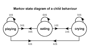
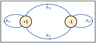
Another convenient way to describe a Markov chain $X$ is through its transition graph. States are indicated by the nodes of the graph, and a strictly positive $(>0)$ transition probability $p_{i j}$ from state $i$ to $j$ is indicated by an arrow from $i$ to $j$ with weight $p_{i j}$.

模拟和蒙特卡洛方法代写

数学代写|模拟和蒙特卡洛方法作业代写模拟和蒙特卡罗方法代考|泊松过程

泊松过程被用来模拟某些类型的到达或模式。想象一下，例如，一台望远镜可以探测到来自遥远星系的单个光子。光子在随机时间到达$T_1, T_2, \ldots$，设$N_t$表示在时间间隔$[0, t]$内到达的数量，即$N_t=\sup \left{k: T_k \leqslant t\right}$。注意，到达间隔$I=(a, b]$中的数量由$N_b-N_a$给出。我们还将用$N(a, b]$来表示它。图1.3给出了到达计数过程$\left{N_t, t \geqslant 0\right}$的示例路径

对于这个特定的到达过程，假设在区间$(a, b)$中到达的数量独立于在区间$(c, d)$中到达的数量，当这两个区间不相交时。这些考虑导致了以下定义:

定义1.12.1(泊松过程)到达计数过程$N=\left{N_t\right}$被称为Pvisson过程，具有规则$\lambda>0$，如果
(a)不重叠区间内的点的数量是独立的
(b)区间$I$中的点的数量具有泊松分布，其平均长度为$\lambda \times$$(I)$ .

数学代写|模拟和蒙特卡洛方法作业代写模拟和蒙特卡罗方法代考|马尔可夫链

考虑一个具有离散(即可数)状态空间$\mathscr{E}$的马尔可夫链$X=\left{X_t, t \in \mathbb{N}\right}$。在本例中，对于所有$x_0, \ldots, x_{t+1}, \in \mathscr{E}$和$t \in \mathbb{N}$，马尔可夫属性$(1.30)$是
$$
\mathbb{P}\left(X_{t+1}=x_{t+1} \mid X_0=x_0, \ldots, X_t=x_t\right)=\mathbb{P}\left(X_{t+1}=x_{t+1} \mid X_t=x_t\right)
$$
。我们将自己限制在马尔可夫链中，其中条件概率
$$
\mathbb{P}\left(X_{t+1}=j \mid X_t=i\right), \quad i, j \in \mathscr{E}
$$与时间$t$无关。这样的链被称为时间同质链。(1.32)中的概率称为$X$的(一步)转移概率。$X_0$的分布称为马尔可夫链的初始分布。一步转移概率和初始分布完全指定了$X$的分布。即，根据乘积法则(1.4)和马尔可夫性质$(1.30)$
$$
\begin{aligned}
&\mathbb{P}\left(X_0=x_0, \ldots, X_t=x_t\right) \
&\quad=\mathbb{P}\left(X_0=x_0\right) \mathbb{P}\left(X_1=x_1 \mid X_0=x_0\right) \cdots \mathbb{P}\left(X_t=x_t \mid X_0=x_0, \ldots X_{t-1}=x_{t-1}\right) \
&\quad=\mathbb{P}\left(X_0=x_0\right) \mathbb{P}\left(X_1=x_1 \mid X_0=x_0\right) \cdots \mathbb{P}\left(X_t=x_t \mid X_{t-1}=x_{t-1}\right) .
\end{aligned}
$$
由于$\mathscr{E}$是可数的，我们可以将一步跃迁概率排列在一个数组中。这个数组称为$X$的(一步)转换矩阵。我们通常用$P$来表示它。例如，当$\mathscr{E}={0,1,2, \ldots}$时，转换矩阵$P$的形式为
$$
P=\left(\begin{array}{cccc}
p_{00} & p_{01} & p_{02} & \ldots \
p_{10} & p_{11} & p_{12} & \ldots \
p_{20} & p_{21} & p_{22} & \ldots \
\vdots & \vdots & \vdots & \ddots
\end{array}\right) .
$$
注意，每一行中的元素都是正的，并求和为单位。描述马尔可夫链的另一种方便的方法是通过它的过渡图$X$。状态由图的节点表示，从状态$i$到$j$的严格正$(>0)$转移概率$p_{i j}$由从$i$到$j$的箭头表示，其权重为$p_{i j}$。

统计代写请认准statistics-lab™. statistics-lab™为您的留学生涯保驾护航。

随机过程代考

在概率论概念中，随机过程是随机变量的集合。 若一随机系统的样本点是随机函数，则称此函数为样本函数，这一随机系统全部样本函数的集合是一个随机过程。 实际应用中，样本函数的一般定义在时间域或者空间域。 随机过程的实例如股票和汇率的波动、语音信号、视频信号、体温的变化，随机运动如布朗运动、随机徘徊等等。

贝叶斯方法代考

贝叶斯统计概念及数据分析表示使用概率陈述回答有关未知参数的研究问题以及统计范式。后验分布包括关于参数的先验分布，和基于观测数据提供关于参数的信息似然模型。根据选择的先验分布和似然模型，后验分布可以解析或近似，例如，马尔科夫链蒙特卡罗 (MCMC) 方法之一。贝叶斯统计概念及数据分析使用后验分布来形成模型参数的各种摘要，包括点估计，如后验平均值、中位数、百分位数和称为可信区间的区间估计。此外，所有关于模型参数的统计检验都可以表示为基于估计后验分布的概率报表。

广义线性模型代考

广义线性模型（GLM）归属统计学领域，是一种应用灵活的线性回归模型。该模型允许因变量的偏差分布有除了正态分布之外的其它分布。

statistics-lab作为专业的留学生服务机构，多年来已为美国、英国、加拿大、澳洲等留学热门地的学生提供专业的学术服务，包括但不限于Essay代写，Assignment代写，Dissertation代写，Report代写，小组作业代写，Proposal代写，Paper代写，Presentation代写，计算机作业代写，论文修改和润色，网课代做，exam代考等等。写作范围涵盖高中，本科，研究生等海外留学全阶段，辐射金融，经济学，会计学，审计学，管理学等全球99%专业科目。写作团队既有专业英语母语作者，也有海外名校硕博留学生，每位写作老师都拥有过硬的语言能力，专业的学科背景和学术写作经验。我们承诺100%原创，100%专业，100%准时，100%满意。

机器学习代写

随着AI的大潮到来，Machine Learning逐渐成为一个新的学习热点。同时与传统CS相比，Machine Learning在其他领域也有着广泛的应用，因此这门学科成为不仅折磨CS专业同学的“小恶魔”，也是折磨生物、化学、统计等其他学科留学生的“大魔王”。学习Machine learning的一大绊脚石在于使用语言众多，跨学科范围广，所以学习起来尤其困难。但是不管你在学习Machine Learning时遇到任何难题，StudyGate专业导师团队都能为你轻松解决。

多元统计分析代考

基础数据: $N$ 个样本， $P$ 个变量数的单样本，组成的横列的数据表
变量定性: 分类和顺序；变量定量：数值
数学公式的角度分为: 因变量与自变量

时间序列分析代写

随机过程，是依赖于参数的一组随机变量的全体，参数通常是时间。 随机变量是随机现象的数量表现，其时间序列是一组按照时间发生先后顺序进行排列的数据点序列。通常一组时间序列的时间间隔为一恒定值（如1秒，5分钟，12小时，7天，1年），因此时间序列可以作为离散时间数据进行分析处理。研究时间序列数据的意义在于现实中，往往需要研究某个事物其随时间发展变化的规律。这就需要通过研究该事物过去发展的历史记录，以得到其自身发展的规律。

回归分析代写

多元回归分析渐进（Multiple Regression Analysis Asymptotics）属于计量经济学领域，主要是一种数学上的统计分析方法，可以分析复杂情况下各影响因素的数学关系，在自然科学、社会和经济学等多个领域内应用广泛。

MATLAB代写

MATLAB 是一种用于技术计算的高性能语言。它将计算、可视化和编程集成在一个易于使用的环境中，其中问题和解决方案以熟悉的数学符号表示。典型用途包括：数学和计算算法开发建模、仿真和原型制作数据分析、探索和可视化科学和工程图形应用程序开发，包括图形用户界面构建MATLAB 是一个交互式系统，其基本数据元素是一个不需要维度的数组。这使您可以解决许多技术计算问题，尤其是那些具有矩阵和向量公式的问题，而只需用 C 或 Fortran 等标量非交互式语言编写程序所需的时间的一小部分。MATLAB 名称代表矩阵实验室。MATLAB 最初的编写目的是提供对由 LINPACK 和 EISPACK 项目开发的矩阵软件的轻松访问，这两个项目共同代表了矩阵计算软件的最新技术。MATLAB 经过多年的发展，得到了许多用户的投入。在大学环境中，它是数学、工程和科学入门和高级课程的标准教学工具。在工业领域，MATLAB 是高效研究、开发和分析的首选工具。MATLAB 具有一系列称为工具箱的特定于应用程序的解决方案。对于大多数 MATLAB 用户来说非常重要，工具箱允许您学习和应用专业技术。工具箱是 MATLAB 函数（M 文件）的综合集合，可扩展 MATLAB 环境以解决特定类别的问题。可用工具箱的领域包括信号处理、控制系统、神经网络、模糊逻辑、小波、仿真等。

R语言代写	问卷设计与分析代写
PYTHON代写	回归分析与线性模型代写
MATLAB代写	方差分析与试验设计代写
STATA代写	机器学习/统计学习代写
SPSS代写	计量经济学代写
EVIEWS代写	时间序列分析代写
EXCEL代写	深度学习代写
SQL代写	各种数据建模与可视化代写

如果你也在 怎样代写模拟和蒙特卡洛方法simulation and monte carlo method这个学科遇到相关的难题，请随时右上角联系我们的24/7代写客服。

蒙特卡洛模拟是一种用于预测随机变量潜力时各种结果的概率的模型。蒙特卡洛模拟有助于解释预测和预报模型中风险和不确定性的影响。

statistics-lab™ 为您的留学生涯保驾护航 在代写模拟和蒙特卡洛方法simulation and monte carlo method方面已经树立了自己的口碑, 保证靠谱, 高质且原创的统计Statistics代写服务。我们的专家在代写模拟和蒙特卡洛方法simulation and monte carlo method代写方面经验极为丰富，各种代写模拟和蒙特卡洛方法simulation and monte carlo method相关的作业也就用不着说。

我们提供的模拟和蒙特卡洛方法simulation and monte carlo method及其相关学科的代写，服务范围广, 其中包括但不限于:

• Statistical Inference 统计推断
• Statistical Computing 统计计算
• Advanced Probability Theory 高等楖率论
• Advanced Mathematical Statistics 高等数理统计学
• (Generalized) Linear Models 广义线性模型
• Statistical Machine Learning 统计机器学习
• Longitudinal Data Analysis 纵向数据分析
• Foundations of Data Science 数据科学基础

数学代写|模拟和蒙特卡洛方法作业代写simulation and monte carlo method代考|RANDOM VARIABLES AND PROBABILITY DISTRIBUTIONS

Specifying a model for a random experiment via a complete description of $\Omega$ and $\mathbb{P}$ may not always be convenient or necessary. In practice, we are only interested in certain observations (i.e., numerical measurements) in the experiment. We incorporate these into our modeling process via the introduction of random variables, usually denoted by capital letters from the last part of the alphabet (e.g., $X$, $\left.X_1, X_2, \ldots, Y, Z\right)$

We toss a biased coin $n$ times, with $p$ the probability of heads. Suppose that we are interested only in the number of heads, say $X$. Note that $X$ can take any of the values in ${0,1, \ldots, n}$. The probability distribution of $X$ is given by the binomial formula
$$
\mathbb{P}(X-k)-\left(\begin{array}{l}
n \
k
\end{array}\right) p^k(1-p)^{n-k}, \quad k-0,1, \ldots, n .
$$
Namely, by Example 1.1, each elementary event ${H T H \cdots T}$ with exactly $k$ heads and $n-k$ tails has probability $p^k(1-p)^{n-k}$, and there are $\left(\begin{array}{l}n \ k\end{array}\right)$ such events.

The probability distribution of a general random variable $X$ – identifying such probabilities as $\mathbb{P}(X=x), \mathbb{P}(a \leqslant X \leqslant b)$, and so on – is completely specified by the cumulative distribution function (cdf), defined by
$$
F(x)=\mathbb{P}(X \leqslant x), x \in \mathbb{R} .
$$
A random variable $X$ is said to have a discrete distribution if, for some finite or countable set of values $x_1, x_2, \ldots, \mathbb{P}\left(X=x_i\right)>0, i=1,2, \ldots$ and $\sum_i \mathbb{P}\left(X=x_i\right)=$ 1. The function $f(x)=\mathbb{P}(X=x)$ is called the probability mass function (pmf) of $X$ – hut see Remark 1.4.1.

数学代写|模拟和蒙特卡洛方法作业代写simulation and monte carlo method代考|JOINT DISTRIBUTIONS

Often a random experiment is described by more than one random variable. The theory for multiple random variables is similar to that for a single random variable.

Let $X_1, \ldots, X_n$ be random variables describing some random experiment. We can accumulate these into a random vector $\mathbf{X}=\left(X_1, \ldots, X_n\right)$. More generally, a collection $\left{X_t, t \in \mathscr{T}\right}$ of random variables is called a stochastic process. The set $\mathscr{T}$ is called the parameter set or index set of the process. It may be discrete (e.g., $\mathbb{N}$ or ${1, \ldots, 10}$ ) or continuous (e.g., $\mathbb{R}{+}=[0, \infty)$ or $\left.[1,10]\right)$. The set of possible values for the stochastic process is called the state space. The joint distribution of $X_1, \ldots, X_n$ is specified by the joint cdf $$ F\left(x_1, \ldots, x_n\right)=\mathbb{P}\left(X_1 \leqslant x_1, \ldots, X_n \leqslant x_n\right) . $$ The joint pdf $f$ is given, in the discrete case, by $f\left(x_1, \ldots, x_n\right)=\mathbb{P}\left(X_1=\right.$ $\left.x_1, \ldots, X_n=x_n\right)$, and in the continuous case $f$ is such that $$ \mathbb{P}(\mathbf{X} \in \mathscr{B})=\int{\mathscr{B}} f\left(x_1, \ldots, x_n\right) \mathrm{d} x_1 \ldots \mathrm{d} x_n
$$
for any (measurable) region $\mathscr{B}$ in $\mathbb{R}^n$. The marginal pdfs can be recovered from the joint pdf by integration or summation. For example, in the case of a continuous random vector $(X, Y)$ with joint pdf $f$, the pdf $f_X$ of $X$ is found as
$$
f_X(x)=\int f(x, y) \mathrm{d} y .
$$
Suppose that $X$ and $Y$ are both discrete or both continuous, with joint pdf $f$, and suppose that $f_X(x)>0$. Then the conditional pdf of $Y$ given $X=x$ is given by
$$
f_{Y \mid X}(y \mid x)=\frac{f(x, y)}{f_X(x)} \quad \text { for all } y .
$$
The corresponding conditional expectation is (in the continuous case)
$$
\mathbb{E}[Y \mid X=x]=\int y f_{Y \mid X}(y \mid x) \mathrm{d} y .
$$
Note that $\mathbb{E}[Y \mid X=x]$ is a function of $x$, say $h(x)$. The corresponding random variable $h(X)$ is written as $\mathbb{E}[Y \mid X]$. It can be shown (see, for example, [3]) that its expectation is simply the expectation of $Y$, that is,
$$
\mathbb{E}[\mathbb{E}[Y \mid X]]=\mathbb{E}[Y]
$$

模拟和蒙特卡洛方法代写

数学代写|模拟和蒙特卡洛方法作业代写模拟和蒙特卡罗方法代考|随机变量和概率分布

通过对$\Omega$和$\mathbb{P}$的完整描述为随机实验指定一个模型可能并不总是方便或必要的。实际上，我们只对实验中的某些观察结果(即数值测量)感兴趣。我们通过引入随机变量将这些变量合并到我们的建模过程中，这些随机变量通常用字母表最后部分的大写字母表示(例如，$X$, $\left.X_1, X_2, \ldots, Y, Z\right)$

)

我们抛一枚有偏见的硬币$n$次，正面出现的概率为$p$。假设我们只对正面的次数感兴趣，比如$X$。注意，$X$可以接受${0,1, \ldots, n}$中的任何值。$X$的概率分布由二项式公式
$$
\mathbb{P}(X-k)-\left(\begin{array}{l}
n \
k
\end{array}\right) p^k(1-p)^{n-k}, \quad k-0,1, \ldots, n .
$$
即，在例1.1中，每个基本事件${H T H \cdots T}$恰好有$k$个正面和$n-k$个反面，其概率为$p^k(1-p)^{n-k}$，有$\left(\begin{array}{l}n \ k\end{array}\right)$个这样的事件

一般随机变量$X$的概率分布-识别诸如$\mathbb{P}(X=x), \mathbb{P}(a \leqslant X \leqslant b)$等的概率-完全由累积分布函数(cdf)指定，由
$$
F(x)=\mathbb{P}(X \leqslant x), x \in \mathbb{R} .
$$
定义一个随机变量$X$被认为具有离散分布，如果，对于某些有限或可数的值集$x_1, x_2, \ldots, \mathbb{P}\left(X=x_i\right)>0, i=1,2, \ldots$和$\sum_i \mathbb{P}\left(X=x_i\right)=$ 1。函数$f(x)=\mathbb{P}(X=x)$被称为$X$ -的概率质量函数(pmf)，请参见注释1.4.1

数学代写|模拟和蒙特卡洛方法作业代写模拟和蒙特卡罗方法代考|联合分布

.

一个随机实验通常由多个随机变量描述。多随机变量的理论与单随机变量的理论相似

让 $X_1, \ldots, X_n$ 是描述随机实验的随机变量。我们可以把这些累加到一个随机向量中 $\mathbf{X}=\left(X_1, \ldots, X_n\right)$。更一般地说，是集合 $\left{X_t, t \in \mathscr{T}\right}$ 的随机变量称为随机过程。布景 $\mathscr{T}$ 称为流程的参数集或索引集。它可能是离散的(例如， $\mathbb{N}$ 或 ${1, \ldots, 10}$ )或连续的(例如， $\mathbb{R}{+}=[0, \infty)$ 或 $\left.[1,10]\right)$。随机过程的可能值集合称为状态空间。的联合分布 $X_1, \ldots, X_n$ 是由联合CDF指定的吗 $$ F\left(x_1, \ldots, x_n\right)=\mathbb{P}\left(X_1 \leqslant x_1, \ldots, X_n \leqslant x_n\right) . $$ 联合pdf $f$ 在离散的情况下，由 $f\left(x_1, \ldots, x_n\right)=\mathbb{P}\left(X_1=\right.$ $\left.x_1, \ldots, X_n=x_n\right)$，在连续情况下 $f$ 是这样的 $$ \mathbb{P}(\mathbf{X} \in \mathscr{B})=\int{\mathscr{B}} f\left(x_1, \ldots, x_n\right) \mathrm{d} x_1 \ldots \mathrm{d} x_n
$$
对于任何(可测量的)区域 $\mathscr{B}$ 在 $\mathbb{R}^n$。边缘pdf可以通过积分或求和的方法从关节pdf中得到。例如，在连续随机向量的情况下 $(X, Y)$ 使用联合PDF $f$， PDF $f_X$ 的 $X$
$$
f_X(x)=\int f(x, y) \mathrm{d} y .
$$
假设 $X$ 和 $Y$ 都是离散的还是连续的，都是联合PDF $f$，假设 $f_X(x)>0$。的条件pdf $Y$ 给定 $X=x$
$$
f_{Y \mid X}(y \mid x)=\frac{f(x, y)}{f_X(x)} \quad \text { for all } y .
$$对应的条件期望(在连续情况下)
$$
\mathbb{E}[Y \mid X=x]=\int y f_{Y \mid X}(y \mid x) \mathrm{d} y .
$$
注意 $\mathbb{E}[Y \mid X=x]$ 是一个函数 $x$，说 $h(x)$。对应的随机变量 $h(X)$ 被写成 $\mathbb{E}[Y \mid X]$。它可以表示(例如，参见[3])它的期望就是的期望 $Y$，即
$$
\mathbb{E}[\mathbb{E}[Y \mid X]]=\mathbb{E}[Y]
$$

统计代写请认准statistics-lab™. statistics-lab™为您的留学生涯保驾护航。

随机过程代考

在概率论概念中，随机过程是随机变量的集合。 若一随机系统的样本点是随机函数，则称此函数为样本函数，这一随机系统全部样本函数的集合是一个随机过程。 实际应用中，样本函数的一般定义在时间域或者空间域。 随机过程的实例如股票和汇率的波动、语音信号、视频信号、体温的变化，随机运动如布朗运动、随机徘徊等等。

贝叶斯方法代考

贝叶斯统计概念及数据分析表示使用概率陈述回答有关未知参数的研究问题以及统计范式。后验分布包括关于参数的先验分布，和基于观测数据提供关于参数的信息似然模型。根据选择的先验分布和似然模型，后验分布可以解析或近似，例如，马尔科夫链蒙特卡罗 (MCMC) 方法之一。贝叶斯统计概念及数据分析使用后验分布来形成模型参数的各种摘要，包括点估计，如后验平均值、中位数、百分位数和称为可信区间的区间估计。此外，所有关于模型参数的统计检验都可以表示为基于估计后验分布的概率报表。

广义线性模型代考

广义线性模型（GLM）归属统计学领域，是一种应用灵活的线性回归模型。该模型允许因变量的偏差分布有除了正态分布之外的其它分布。

statistics-lab作为专业的留学生服务机构，多年来已为美国、英国、加拿大、澳洲等留学热门地的学生提供专业的学术服务，包括但不限于Essay代写，Assignment代写，Dissertation代写，Report代写，小组作业代写，Proposal代写，Paper代写，Presentation代写，计算机作业代写，论文修改和润色，网课代做，exam代考等等。写作范围涵盖高中，本科，研究生等海外留学全阶段，辐射金融，经济学，会计学，审计学，管理学等全球99%专业科目。写作团队既有专业英语母语作者，也有海外名校硕博留学生，每位写作老师都拥有过硬的语言能力，专业的学科背景和学术写作经验。我们承诺100%原创，100%专业，100%准时，100%满意。

机器学习代写

随着AI的大潮到来，Machine Learning逐渐成为一个新的学习热点。同时与传统CS相比，Machine Learning在其他领域也有着广泛的应用，因此这门学科成为不仅折磨CS专业同学的“小恶魔”，也是折磨生物、化学、统计等其他学科留学生的“大魔王”。学习Machine learning的一大绊脚石在于使用语言众多，跨学科范围广，所以学习起来尤其困难。但是不管你在学习Machine Learning时遇到任何难题，StudyGate专业导师团队都能为你轻松解决。

多元统计分析代考

基础数据: $N$ 个样本， $P$ 个变量数的单样本，组成的横列的数据表
变量定性: 分类和顺序；变量定量：数值
数学公式的角度分为: 因变量与自变量

时间序列分析代写

随机过程，是依赖于参数的一组随机变量的全体，参数通常是时间。 随机变量是随机现象的数量表现，其时间序列是一组按照时间发生先后顺序进行排列的数据点序列。通常一组时间序列的时间间隔为一恒定值（如1秒，5分钟，12小时，7天，1年），因此时间序列可以作为离散时间数据进行分析处理。研究时间序列数据的意义在于现实中，往往需要研究某个事物其随时间发展变化的规律。这就需要通过研究该事物过去发展的历史记录，以得到其自身发展的规律。

回归分析代写

多元回归分析渐进（Multiple Regression Analysis Asymptotics）属于计量经济学领域，主要是一种数学上的统计分析方法，可以分析复杂情况下各影响因素的数学关系，在自然科学、社会和经济学等多个领域内应用广泛。

MATLAB代写

MATLAB 是一种用于技术计算的高性能语言。它将计算、可视化和编程集成在一个易于使用的环境中，其中问题和解决方案以熟悉的数学符号表示。典型用途包括：数学和计算算法开发建模、仿真和原型制作数据分析、探索和可视化科学和工程图形应用程序开发，包括图形用户界面构建MATLAB 是一个交互式系统，其基本数据元素是一个不需要维度的数组。这使您可以解决许多技术计算问题，尤其是那些具有矩阵和向量公式的问题，而只需用 C 或 Fortran 等标量非交互式语言编写程序所需的时间的一小部分。MATLAB 名称代表矩阵实验室。MATLAB 最初的编写目的是提供对由 LINPACK 和 EISPACK 项目开发的矩阵软件的轻松访问，这两个项目共同代表了矩阵计算软件的最新技术。MATLAB 经过多年的发展，得到了许多用户的投入。在大学环境中，它是数学、工程和科学入门和高级课程的标准教学工具。在工业领域，MATLAB 是高效研究、开发和分析的首选工具。MATLAB 具有一系列称为工具箱的特定于应用程序的解决方案。对于大多数 MATLAB 用户来说非常重要，工具箱允许您学习和应用专业技术。工具箱是 MATLAB 函数（M 文件）的综合集合，可扩展 MATLAB 环境以解决特定类别的问题。可用工具箱的领域包括信号处理、控制系统、神经网络、模糊逻辑、小波、仿真等。

R语言代写	问卷设计与分析代写
PYTHON代写	回归分析与线性模型代写
MATLAB代写	方差分析与试验设计代写
STATA代写	机器学习/统计学习代写
SPSS代写	计量经济学代写
EVIEWS代写	时间序列分析代写
EXCEL代写	深度学习代写
SQL代写	各种数据建模与可视化代写

如果你也在 怎样代写模拟和蒙特卡洛方法simulation and monte carlo method这个学科遇到相关的难题，请随时右上角联系我们的24/7代写客服。

蒙特卡洛模拟是一种用于预测随机变量潜力时各种结果的概率的模型。蒙特卡洛模拟有助于解释预测和预报模型中风险和不确定性的影响。

statistics-lab™ 为您的留学生涯保驾护航 在代写模拟和蒙特卡洛方法simulation and monte carlo method方面已经树立了自己的口碑, 保证靠谱, 高质且原创的统计Statistics代写服务。我们的专家在代写模拟和蒙特卡洛方法simulation and monte carlo method代写方面经验极为丰富，各种代写模拟和蒙特卡洛方法simulation and monte carlo method相关的作业也就用不着说。

我们提供的模拟和蒙特卡洛方法simulation and monte carlo method及其相关学科的代写，服务范围广, 其中包括但不限于:

• Statistical Inference 统计推断
• Statistical Computing 统计计算
• Advanced Probability Theory 高等楖率论
• Advanced Mathematical Statistics 高等数理统计学
• (Generalized) Linear Models 广义线性模型
• Statistical Machine Learning 统计机器学习
• Longitudinal Data Analysis 纵向数据分析
• Foundations of Data Science 数据科学基础

数学代写|模拟和蒙特卡洛方法作业代写simulation and monte carlo method代考|RANDOM EXPERIMENTS

The basic notion in probability theory is that of a random experiment: an experiment whose outcome cannot be determined in advance. The most fundamental example is the experiment where a fair coin is tossed a number of times. For simplicity suppose that the coin is tossed three times. The sample space, denoted $\Omega$, is the set of all possible outcomes of the experiment. In this case $\Omega$ has eight possible outcomes:
$$
\Omega={H H H, H H T, H T H, H T T, T H H, T H T, T T H, T T T},
$$
where, for example, HTH means that the first toss is heads, the second tails, and the third heads.

Subsets of the sample space are called events. For example, the event $A$ that the third toss is heads is
$A={H H H, H T H, T H H, T T H}$
We say that event $A$ occurs if the outcome of the experiment is one of the elements in $A$. Since events are sets, we can apply the usual set operations to them. For example, the event $A \cup B$, called the union of $A$ and $B$, is the event that $A$ or $B$ or both occur, and the event $A \cap B$, called the intersection of $A$ and $B$, is the event that $A$ and $B$ both occur. Similar notation holds for unions and intersections of more than two events. The event $A^c$, called the complement of $A$, is the event that $A$ does not occur. Two events $A$ and $B$ that have no outcomes in common, that is, their intersection is empty, are called disjoint events. The main step is to specify the probability of each event.

Definition 1.2.1 (Probability) A probability $\mathbb{P}$ is a rule that assigns a number $0 \leqslant \mathbb{P}(A) \leqslant 1$ to each event $A$, such that $\mathbb{P}(\Omega)=1$, and such that for any sequence $A_1, A_2, \ldots$ of disjoint events
$$
\mathbb{P}\left(\bigcup_i A_i\right)=\sum_i \mathbb{P}\left(A_i\right) .
$$
Equation (1.1) is referred to as the sum rule of probability. It states that if an event can happen in a number of different ways, but not simultaneously, the probability of that event is simply the sum of the probabilities of the comprising events.

For the fair coin toss experiment the probability of any event is easily given. Namely, because the coin is fair, each of the eight possible outcomes is equally likely, so that $\mathbb{P}({H H H})=\cdots=\mathbb{P}({T T T})=1 / 8$. Since any event $A$ is the union of the “elementary” events ${H H H}, \ldots,{T T T}$, the sum rule implies that
$$
\mathbb{P}(A)=\frac{|A|}{|\Omega|},
$$
where $|A|$ denotes the number of outcomes in $A$ and $|\Omega|=8$. More generally, if a random experiment has finitely many and equally likely outcomes, the probability is always of the form (1.2). In that case the calculation of probabilities reduces to counting.

数学代写|模拟和蒙特卡洛方法作业代写simulation and monte carlo method代考|CONDITIONAL PROBABILITY AND INDEPENDENCE

How do probabilities change when we know that some event $B \subset \Omega$ has occurred? Given that the outcome lies in $B$, the event $A$ will occur if and only if $A \cap B$ occurs, and the relative chance of $A$ occurring is therefore $\mathbb{P}(A \cap B) / \mathbb{P}(B)$. This leads to the definition of the conditional probability of $A$ given $B$ :
$$
\mathbb{P}(A \mid B)=\frac{\mathbb{P}(A \cap B)}{\mathbb{P}(B)} .
$$
For example, suppose that we toss a fair coin three times. Let $B$ be the event that the total number of heads is two. The conditional probability of the event $A$ that the first toss is heads, given that $B$ occurs, is $(2 / 8) /(3 / 8)=2 / 3$.

Rewriting (1.3) and interchanging the role of $A$ and $B$ gives the relation $\mathbb{P}(A \cap$ $B)=\mathbb{P}(A) \mathbb{P}(B \mid A)$. This can be generalized easily to the product rule of probability, which states that for any sequence of events $A_1, A_2, \ldots, A_n$,
$$
\mathbb{P}\left(A_1 \cdots A_n\right)=\mathbb{P}\left(A_1\right) \mathbb{P}\left(A_2 \mid A_1\right) \mathbb{P}\left(A_3 \mid A_1 A_2\right) \cdots \mathbb{P}\left(A_n \mid A_1 \cdots A_{n-1}\right),
$$
using the abbreviation $A_1 A_2 \cdots A_k \equiv A_1 \cap A_2 \cap \cdots \cap A_k$.
Suppose that $B_1, B_2, \ldots, B_n$ is a partition of $\Omega$. That is, $B_1, B_2, \ldots, B_n$ are disjoint and their union is $\Omega$. Then, by the sum rule, $\mathbb{P}(A)=\sum_{i=1}^n \mathbb{P}\left(A \cap B_i\right)$ and hence, by the definition of conditional probability, we have the law of total probability:
$$
\mathbb{P}(A)=\sum_{i=1}^n \mathbb{P}\left(A \mid B_i\right) \mathbb{P}\left(B_i\right)
$$
Combining this with the definition of conditional probability gives Bayes’ rule:
$$
\mathbb{P}\left(B_j \mid A\right)=\frac{\mathbb{P}\left(A \mid B_j\right) \mathbb{P}\left(B_j\right)}{\sum_{i=1}^n \mathbb{P}\left(A \mid B_i\right) \mathbb{P}\left(B_i\right)} .
$$
Independence is of crucial importance in probability and statistics. Loosely speaking, it models the lack of information between events. Two events $A$ and $B$ are said to be independent if the knowledge that $B$ has occurred does not change the probability that $A$ occurs. That is, $A, B$ independent $\Leftrightarrow \mathbb{P}(A \mid B)=\mathbb{P}(A)$. Since $\mathbb{P}(A \mid B)=\mathbb{P}(A \cap B) / \mathbb{P}(B)$, an alternative definition of independence is
$A, B$ independent $\Leftrightarrow \mathbb{P}(A \cap B)=\mathbb{P}(A) \mathbb{P}(B)$
This definition covers the case where $B=\emptyset$ (empty set). We can extend this definition to arbitrarily many events.

模拟和蒙特卡洛方法代写

数学代写|模拟和蒙特卡洛方法作业代写模拟和蒙特卡罗方法代考|随机实验

概率论的基本概念是一个随机实验:一个结果无法事先确定的实验。最基本的例子是一个实验，一个均匀的硬币被抛了很多次。为了简单起见，假设抛硬币三次。样本空间，记为$\Omega$，是实验所有可能结果的集合。在这种情况下，$\Omega$有八种可能的结果:
$$
\Omega={H H H, H H T, H T H, H T T, T H H, T H T, T T H, T T T},
$$
其中，例如，HTH意味着第一次抛掷是正面，第二次是反面，第三次是正面

样本空间的子集称为事件。例如，第三次抛掷是正面的事件$A$是
$A={H H H, H T H, T H H, T T H}$
我们说，如果实验的结果是$A$中的元素之一，则事件$A$发生。由于事件是集合，我们可以对它们应用通常的集合操作。例如，事件$A \cup B$，称为$A$和$B$的并集，是$A$或$B$或两者都发生的事件，事件$A \cap B$，称为$A$和$B$的交集，是$A$和$B$都发生的事件。类似的符号也适用于两个以上事件的合并和交集。事件$A^c$被称为$A$的补充，是$A$没有发生的事件。两个事件$A$和$B$没有共同的结果，即它们的交集为空，称为不相交事件。主要步骤是指定每个事件的概率

定义1.2.1(概率)概率$\mathbb{P}$是给每个事件$A$分配一个数字$0 \leqslant \mathbb{P}(A) \leqslant 1$的规则，使得$\mathbb{P}(\Omega)=1$，并且对于任何不连接事件的序列$A_1, A_2, \ldots$
$$
\mathbb{P}\left(\bigcup_i A_i\right)=\sum_i \mathbb{P}\left(A_i\right) .
$$
公式(1.1)被称为概率和规则。它指出，如果一个事件可以以多种不同的方式发生，但不是同时发生，那么该事件的概率就是构成该事件的所有事件的概率之和

对于公平抛硬币实验，任何事件的概率都很容易给出。也就是说，因为硬币是均匀的，八种可能的结果都是等可能的，所以$\mathbb{P}({H H H})=\cdots=\mathbb{P}({T T T})=1 / 8$。因为任何事件$A$是“基本”事件${H H H}, \ldots,{T T T}$的并集，所以求和规则意味着
$$
\mathbb{P}(A)=\frac{|A|}{|\Omega|},
$$
，其中$|A|$表示$A$和$|\Omega|=8$中的结果数量。更一般地说，如果一个随机实验有有限多个等可能的结果，概率总是形式(1.2)。在这种情况下，概率的计算简化为计数

数学代写|模拟和蒙特卡洛方法作业代写模拟和蒙特卡罗方法代考|条件概率和独立性

当我们知道某个事件$B \subset \Omega$已经发生时，概率是如何变化的?假设结果位于$B$，那么事件$A$将在且仅当$A \cap B$发生时发生，因此$A$发生的相对几率是$\mathbb{P}(A \cap B) / \mathbb{P}(B)$。这导致了条件概率的定义$A$给定$B$:
$$
\mathbb{P}(A \mid B)=\frac{\mathbb{P}(A \cap B)}{\mathbb{P}(B)} .
$$
例如，假设我们投掷一枚均匀硬币三次。设$B$是正面总次数为2的情况。假设$B$发生，第一次抛掷是正面的事件$A$的条件概率是$(2 / 8) /(3 / 8)=2 / 3$ .

重写(1.3)并交换$A$和$B$的角色，得到关系$\mathbb{P}(A \cap$$B)=\mathbb{P}(A) \mathbb{P}(B \mid A)$。这可以很容易地推广到概率积规则，该规则规定，对于任何事件序列$A_1, A_2, \ldots, A_n$，
$$
\mathbb{P}\left(A_1 \cdots A_n\right)=\mathbb{P}\left(A_1\right) \mathbb{P}\left(A_2 \mid A_1\right) \mathbb{P}\left(A_3 \mid A_1 A_2\right) \cdots \mathbb{P}\left(A_n \mid A_1 \cdots A_{n-1}\right),
$$
，使用缩写$A_1 A_2 \cdots A_k \equiv A_1 \cap A_2 \cap \cdots \cap A_k$ .
假设$B_1, B_2, \ldots, B_n$是$\Omega$的一个分区。也就是说，$B_1, B_2, \ldots, B_n$是分离的，它们的并集是$\Omega$。然后，通过求和规则，$\mathbb{P}(A)=\sum_{i=1}^n \mathbb{P}\left(A \cap B_i\right)$，因此，通过条件概率的定义，我们有了全概率定律:
$$
\mathbb{P}(A)=\sum_{i=1}^n \mathbb{P}\left(A \mid B_i\right) \mathbb{P}\left(B_i\right)
$$
结合这个和条件概率的定义，我们得到了贝叶斯规则:
$$
\mathbb{P}\left(B_j \mid A\right)=\frac{\mathbb{P}\left(A \mid B_j\right) \mathbb{P}\left(B_j\right)}{\sum_{i=1}^n \mathbb{P}\left(A \mid B_i\right) \mathbb{P}\left(B_i\right)} .
$$
独立性在概率和统计中是至关重要的。粗略地说，它对事件之间缺乏信息进行了建模。如果知道$B$发生了并不改变$A$发生的概率，则称$A$和$B$两个事件是独立的。即$A, B$独立$\Leftrightarrow \mathbb{P}(A \mid B)=\mathbb{P}(A)$。因为$\mathbb{P}(A \mid B)=\mathbb{P}(A \cap B) / \mathbb{P}(B)$，独立的另一个定义是
$A, B$ independent $\Leftrightarrow \mathbb{P}(A \cap B)=\mathbb{P}(A) \mathbb{P}(B)$
这个定义涵盖了$B=\emptyset$(空集)的情况。我们可以将这个定义扩展到任意多个事件

统计代写请认准statistics-lab™. statistics-lab™为您的留学生涯保驾护航。

随机过程代考

在概率论概念中，随机过程是随机变量的集合。 若一随机系统的样本点是随机函数，则称此函数为样本函数，这一随机系统全部样本函数的集合是一个随机过程。 实际应用中，样本函数的一般定义在时间域或者空间域。 随机过程的实例如股票和汇率的波动、语音信号、视频信号、体温的变化，随机运动如布朗运动、随机徘徊等等。

贝叶斯方法代考

贝叶斯统计概念及数据分析表示使用概率陈述回答有关未知参数的研究问题以及统计范式。后验分布包括关于参数的先验分布，和基于观测数据提供关于参数的信息似然模型。根据选择的先验分布和似然模型，后验分布可以解析或近似，例如，马尔科夫链蒙特卡罗 (MCMC) 方法之一。贝叶斯统计概念及数据分析使用后验分布来形成模型参数的各种摘要，包括点估计，如后验平均值、中位数、百分位数和称为可信区间的区间估计。此外，所有关于模型参数的统计检验都可以表示为基于估计后验分布的概率报表。

广义线性模型代考

广义线性模型（GLM）归属统计学领域，是一种应用灵活的线性回归模型。该模型允许因变量的偏差分布有除了正态分布之外的其它分布。

statistics-lab作为专业的留学生服务机构，多年来已为美国、英国、加拿大、澳洲等留学热门地的学生提供专业的学术服务，包括但不限于Essay代写，Assignment代写，Dissertation代写，Report代写，小组作业代写，Proposal代写，Paper代写，Presentation代写，计算机作业代写，论文修改和润色，网课代做，exam代考等等。写作范围涵盖高中，本科，研究生等海外留学全阶段，辐射金融，经济学，会计学，审计学，管理学等全球99%专业科目。写作团队既有专业英语母语作者，也有海外名校硕博留学生，每位写作老师都拥有过硬的语言能力，专业的学科背景和学术写作经验。我们承诺100%原创，100%专业，100%准时，100%满意。

机器学习代写

随着AI的大潮到来，Machine Learning逐渐成为一个新的学习热点。同时与传统CS相比，Machine Learning在其他领域也有着广泛的应用，因此这门学科成为不仅折磨CS专业同学的“小恶魔”，也是折磨生物、化学、统计等其他学科留学生的“大魔王”。学习Machine learning的一大绊脚石在于使用语言众多，跨学科范围广，所以学习起来尤其困难。但是不管你在学习Machine Learning时遇到任何难题，StudyGate专业导师团队都能为你轻松解决。

多元统计分析代考

基础数据: $N$ 个样本， $P$ 个变量数的单样本，组成的横列的数据表
变量定性: 分类和顺序；变量定量：数值
数学公式的角度分为: 因变量与自变量

时间序列分析代写

随机过程，是依赖于参数的一组随机变量的全体，参数通常是时间。 随机变量是随机现象的数量表现，其时间序列是一组按照时间发生先后顺序进行排列的数据点序列。通常一组时间序列的时间间隔为一恒定值（如1秒，5分钟，12小时，7天，1年），因此时间序列可以作为离散时间数据进行分析处理。研究时间序列数据的意义在于现实中，往往需要研究某个事物其随时间发展变化的规律。这就需要通过研究该事物过去发展的历史记录，以得到其自身发展的规律。

回归分析代写

多元回归分析渐进（Multiple Regression Analysis Asymptotics）属于计量经济学领域，主要是一种数学上的统计分析方法，可以分析复杂情况下各影响因素的数学关系，在自然科学、社会和经济学等多个领域内应用广泛。

MATLAB代写

MATLAB 是一种用于技术计算的高性能语言。它将计算、可视化和编程集成在一个易于使用的环境中，其中问题和解决方案以熟悉的数学符号表示。典型用途包括：数学和计算算法开发建模、仿真和原型制作数据分析、探索和可视化科学和工程图形应用程序开发，包括图形用户界面构建MATLAB 是一个交互式系统，其基本数据元素是一个不需要维度的数组。这使您可以解决许多技术计算问题，尤其是那些具有矩阵和向量公式的问题，而只需用 C 或 Fortran 等标量非交互式语言编写程序所需的时间的一小部分。MATLAB 名称代表矩阵实验室。MATLAB 最初的编写目的是提供对由 LINPACK 和 EISPACK 项目开发的矩阵软件的轻松访问，这两个项目共同代表了矩阵计算软件的最新技术。MATLAB 经过多年的发展，得到了许多用户的投入。在大学环境中，它是数学、工程和科学入门和高级课程的标准教学工具。在工业领域，MATLAB 是高效研究、开发和分析的首选工具。MATLAB 具有一系列称为工具箱的特定于应用程序的解决方案。对于大多数 MATLAB 用户来说非常重要，工具箱允许您学习和应用专业技术。工具箱是 MATLAB 函数（M 文件）的综合集合，可扩展 MATLAB 环境以解决特定类别的问题。可用工具箱的领域包括信号处理、控制系统、神经网络、模糊逻辑、小波、仿真等。

R语言代写	问卷设计与分析代写
PYTHON代写	回归分析与线性模型代写
MATLAB代写	方差分析与试验设计代写
STATA代写	机器学习/统计学习代写
SPSS代写	计量经济学代写
EVIEWS代写	时间序列分析代写
EXCEL代写	深度学习代写
SQL代写	各种数据建模与可视化代写