分类: 流体力学代写

澳洲代写|CIVL3612|Fluid Mechanics流体力学 悉尼大学

statistics-labTM为您悉尼大学(英语:The University of Sydney),简称悉大、USYD,简称“NCL”Business Entrepreneurship: Business Models企业创业: 商业模式澳洲代写代考辅导服务!

课程介绍:

This unit of study aims to provide an understanding of the conservation of mass and momentum in differential forms for viscous fluid flows. It provides the foundation for advanced study of turbulence, flow around immersed bodies, open channel flow, pipe flow and pump design.

澳洲代写|OLET1201|Business Entrepreneurship: Business Models企业创业: 商业模式 悉尼大学
Key InformationDetails
Course NumberCIVL3612
Pre-requisites(Not mentioned in the text)
Academic Unit (Major)Civil Engineering
Instructor(Not mentioned in the text)
Credit Points6

Business Models商业模式问题集

问题 1.

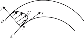
A common observation in big rivers or other fast-flowing bodies of water (e.g. during floods) is shown in the figures and sketch below. A fast moving stream of water that is steadily flowing along suddenly decelerates and the position of the free surface ‘jumps’ upwards. After a lot of local turbulent motion, the flow settles down again but is now steadily moving at a significantly slower speed.

We will represent the free surface height as $h(x)$ and the velocity by the function $u(x)$. The fluid has constant density $\rho$ and we will treat the problem as one-dimensional. You can assume that viscous stresses along the control surfaces of the volume shown above are negligibly small, and neglect the density of air.
PART I:
a) consider a streamline drawn (line $\mathrm{AB}$ in the figure) just above the smooth flat lower surface of the channel. How is the static pressure in the fluid along this line related to the height of the river? How does the static pressure vary along the line DEA?

(a):
The pressure distribution on line $\mathrm{AB}$ follows the hydrostatic rule. It is true that the flow is not static but by picking an arbitrary control volume at any point on line AB (green dashed control volume in Figure 1) one can see that the balance of forces in the $y$-direction will tell us that the difference between the pressure at the bottom and the ambient pressure should balance the weight of the liquid inside the control volume. This simply implies that the static pressure on line $\mathrm{AB}$ should be equal
The pressure distribution on line DEA also follows the hydrostatic change merely due to the fact that there is no curvature in the streamlines as one integrates the Euler equation normal to them and thus the only change in pressure when one moves from $\mathrm{E}$ to A will be the hydrostatic part. Ignoring the density of air one can see that the pressure is constant from D to E and then start to grow linearly with height as we move from $\mathrm{E}$ to $\mathrm{A}$. The result is shown in Figure

问题 2.

b) Using the control volume shown in the sketch develop two expressions that relate the velocity and height of the stream at station 1 and the velocity and height of the stream at station 2. Developing a table of relevant quantities along each face of the control volume ABCDEA is highly recommended!
c) [2 points] Combine your expressions from (a) and (b) together to show that the speed of the river can be simply evaluated from simple measurements of the river height (e.g. using marked yardsticks attached to the channel floor):
$$
u_1=\sqrt{\frac{g h_2}{2 h_1}\left(h_1+h_2\right)}
$$

}(b) and (c): The selected control volume is shown in Figure 3 (dashed green line). One can subtract the ambient pressure from the entire problem and knowing that the net effect of uniform $P_a$ acting on the control volume is zero then there will be no change in the problem analysis if we only deal with gauge pressures $\left(P(x, y)-P_a\right)$Table 1 summarizes all the important parameters acting on different control surfaces for the selected control volume:

Now we can start by writing the conservation rules using the RTT. It is important to notice that due to the turbulent mixing happening in the region of the hydraulic jump, energy will not be conserved and thus either applying the conservation of energy or the Bernoulli equation will not be the right approach. If we write the conservation of mass for the selected control volume then we will have:

$$
\text { C.O.Mass: } 0=\frac{d}{d t} \int_{\text {c.v. }} \rho d V+\int_{\text {c.s. }} \rho\left(v-v_c\right) \cdot n d A
$$

Knowing that the problem is steady state and using the tabulated quantities, conservation of mass can be simplified to:
$\rho u_1 h_1=\rho u_2 h_2 \Rightarrow u_1 h_1=u_2 h_2$
The conservation of linear momentum in the $x$ direction can also be written in the RTT form:

$$
\text { C.O.Momentum: } \frac{1}{W} \sum F_x=\frac{d}{d t} \int_{c . v .} \rho v_x d V+\int_{\text {c.s. }} \rho v_x\left(v-v_c\right) \cdot n d A
$$


where $W$ is the width into the page.
The net of external forces acting in the $x$-direction on the control volume neglecting the wall shear effect is a result of pressure forces acting on the (AD) and (BC) control surfaces:

$$
\frac{1}{W} \sum F_x=\int_{A D}\left(P-P_a\right) d y-\int_{B C}\left(P-P_a\right) d y=\int_0^{h_1} \rho g y d y-\int_0^{h_2} \rho g y d y=\rho g\left(\frac{h_1^2}{2}-\frac{h_2^2}{2}\right)
$$


The right hand side of the RTT for the conservation of linear momentum can also be simplified to (knowing that the problem is steady and using the tabulated identities):

$$
\text { R.H.S. of RTT for C.O. Momentum }=\rho u_2^2 h_2-\rho u_1^2 h_1
$$


thus the conservation of linear momentum implies that:

$$
\rho g\left(\frac{h_1^2}{2}-\frac{h_2^2}{2}\right)=\rho u_2^2 h_2-\rho u_1^2 h_1 \Rightarrow \frac{g}{2}\left(h_1^2-h_2^2\right)=u_2^2 h_2-u_1^2 h_1
$$

using the result from conservation of mass (equation (1)) one can eliminate $u_2$ from equation (2) to give:

$$
\frac{g}{2}\left(h_1^2-h_2^2\right)=h_1 u_1^2\left(h_1 / h_2-1\right) \Rightarrow u_1=\sqrt{\frac{g h_2}{2 h_1}\left(h_1+h_2\right)}
$$


where we have used the identity $h_1^2-h_2^2=\left(h_1-h_2\right)\left(h_1+h_2\right)$.

问题 3.

A deeper question to answer is why is the water moving so fast locally to begin with. To answer this we must consider the topography of the river bed that is upstream of station 1 , as shown in the drawing below. We denote the height of the fluid stream above the river bed as $h(x)$ and the height of the riverbed by $b(x)$ :
d) [1 point] Consider a slice of river $d x$ and show that conservation of mass can be written in the form:
$$
u(x) \frac{d h(x)}{d x}+h(x) \frac{d u(x)}{d x}=0
$$

(d):
For the selected control volume (Figure 4 ) one can easily write the conservation of mass using Taylor series to obtain expressions for $u(x+\Delta x)$ and $h(x+\Delta x)$ :
$$
u(x) h(x)=u(x+\Delta x) h(x+\Delta x) \rightarrow u(x) h(x)=\left(u(x)+\frac{d u}{d x} \Delta x\right)\left(h(x)+\frac{d h}{d x} \Delta x\right)
$$
which after ignoring the second order terms such $\left(\Delta x^2\right)$ it can be rewritten as:
$$
\Delta x\left(u(x) \frac{d h}{d x}+h(x) \frac{d u}{d x}\right)=0 \Rightarrow u \frac{d h}{d x}+h \frac{d u}{d x}=0
$$
Another way to reach the same result is to say that since the flow is incompressible then the volumetric flow rate should remain unchanged thus $d(u h) / d x=0$ which will lead to the same result we just derived in equation (4).

Figure 4: An arbitrary control volume selected to derive the conservation of mass in the differential form.

统计代写请认准statistics-lab™. statistics-lab™为您的留学生涯保驾护航。

金融工程代写

金融工程是使用数学技术来解决金融问题。金融工程使用计算机科学、统计学、经济学和应用数学领域的工具和知识来解决当前的金融问题,以及设计新的和创新的金融产品。

非参数统计代写

非参数统计指的是一种统计方法,其中不假设数据来自于由少数参数决定的规定模型;这种模型的例子包括正态分布模型和线性回归模型。

广义线性模型代考

广义线性模型(GLM)归属统计学领域,是一种应用灵活的线性回归模型。该模型允许因变量的偏差分布有除了正态分布之外的其它分布。

术语 广义线性模型(GLM)通常是指给定连续和/或分类预测因素的连续响应变量的常规线性回归模型。它包括多元线性回归,以及方差分析和方差分析(仅含固定效应)。

有限元方法代写

有限元方法(FEM)是一种流行的方法,用于数值解决工程和数学建模中出现的微分方程。典型的问题领域包括结构分析、传热、流体流动、质量运输和电磁势等传统领域。

有限元是一种通用的数值方法,用于解决两个或三个空间变量的偏微分方程(即一些边界值问题)。为了解决一个问题,有限元将一个大系统细分为更小、更简单的部分,称为有限元。这是通过在空间维度上的特定空间离散化来实现的,它是通过构建对象的网格来实现的:用于求解的数值域,它有有限数量的点。边界值问题的有限元方法表述最终导致一个代数方程组。该方法在域上对未知函数进行逼近。[1] 然后将模拟这些有限元的简单方程组合成一个更大的方程系统,以模拟整个问题。然后,有限元通过变化微积分使相关的误差函数最小化来逼近一个解决方案。

tatistics-lab作为专业的留学生服务机构,多年来已为美国、英国、加拿大、澳洲等留学热门地的学生提供专业的学术服务,包括但不限于Essay代写,Assignment代写,Dissertation代写,Report代写,小组作业代写,Proposal代写,Paper代写,Presentation代写,计算机作业代写,论文修改和润色,网课代做,exam代考等等。写作范围涵盖高中,本科,研究生等海外留学全阶段,辐射金融,经济学,会计学,审计学,管理学等全球99%专业科目。写作团队既有专业英语母语作者,也有海外名校硕博留学生,每位写作老师都拥有过硬的语言能力,专业的学科背景和学术写作经验。我们承诺100%原创,100%专业,100%准时,100%满意。

随机分析代写


随机微积分是数学的一个分支,对随机过程进行操作。它允许为随机过程的积分定义一个关于随机过程的一致的积分理论。这个领域是由日本数学家伊藤清在第二次世界大战期间创建并开始的。

时间序列分析代写

随机过程,是依赖于参数的一组随机变量的全体,参数通常是时间。 随机变量是随机现象的数量表现,其时间序列是一组按照时间发生先后顺序进行排列的数据点序列。通常一组时间序列的时间间隔为一恒定值(如1秒,5分钟,12小时,7天,1年),因此时间序列可以作为离散时间数据进行分析处理。研究时间序列数据的意义在于现实中,往往需要研究某个事物其随时间发展变化的规律。这就需要通过研究该事物过去发展的历史记录,以得到其自身发展的规律。

回归分析代写

多元回归分析渐进(Multiple Regression Analysis Asymptotics)属于计量经济学领域,主要是一种数学上的统计分析方法,可以分析复杂情况下各影响因素的数学关系,在自然科学、社会和经济学等多个领域内应用广泛。

MATLAB代写

MATLAB 是一种用于技术计算的高性能语言。它将计算、可视化和编程集成在一个易于使用的环境中,其中问题和解决方案以熟悉的数学符号表示。典型用途包括:数学和计算算法开发建模、仿真和原型制作数据分析、探索和可视化科学和工程图形应用程序开发,包括图形用户界面构建MATLAB 是一个交互式系统,其基本数据元素是一个不需要维度的数组。这使您可以解决许多技术计算问题,尤其是那些具有矩阵和向量公式的问题,而只需用 C 或 Fortran 等标量非交互式语言编写程序所需的时间的一小部分。MATLAB 名称代表矩阵实验室。MATLAB 最初的编写目的是提供对由 LINPACK 和 EISPACK 项目开发的矩阵软件的轻松访问,这两个项目共同代表了矩阵计算软件的最新技术。MATLAB 经过多年的发展,得到了许多用户的投入。在大学环境中,它是数学、工程和科学入门和高级课程的标准教学工具。在工业领域,MATLAB 是高效研究、开发和分析的首选工具。MATLAB 具有一系列称为工具箱的特定于应用程序的解决方案。对于大多数 MATLAB 用户来说非常重要,工具箱允许您学习应用专业技术。工具箱是 MATLAB 函数(M 文件)的综合集合,可扩展 MATLAB 环境以解决特定类别的问题。可用工具箱的领域包括信号处理、控制系统、神经网络、模糊逻辑、小波、仿真等。

R语言代写问卷设计与分析代写
PYTHON代写回归分析与线性模型代写
MATLAB代写方差分析与试验设计代写
STATA代写机器学习/统计学习代写
SPSS代写计量经济学代写
EVIEWS代写时间序列分析代写
EXCEL代写深度学习代写
SQL代写各种数据建模与可视化代写

物理代写|流体力学代写Fluid Mechanics代考|One-Equation Model by Prandtl

如果你也在 怎样代写流体力学Fluid Mechanics这个学科遇到相关的难题,请随时右上角联系我们的24/7代写客服。

流体力学是物理学的一个分支,涉及流体(液体、气体和等离子体)的力学和对它们的力。它的应用范围很广,包括机械、土木工程、化学和生物医学工程、地球物理学、海洋学、气象学、天体物理学和生物学。

statistics-lab™ 为您的留学生涯保驾护航 在代写流体力学Fluid Mechanics方面已经树立了自己的口碑, 保证靠谱, 高质且原创的统计Statistics代写服务。我们的专家在代写流体力学Fluid Mechanics代写方面经验极为丰富,各种代写流体力学Fluid Mechanics相关的作业也就用不着说。

我们提供的流体力学Fluid Mechanics及其相关学科的代写,服务范围广, 其中包括但不限于:

  • Statistical Inference 统计推断
  • Statistical Computing 统计计算
  • Advanced Probability Theory 高等概率论
  • Advanced Mathematical Statistics 高等数理统计学
  • (Generalized) Linear Models 广义线性模型
  • Statistical Machine Learning 统计机器学习
  • Longitudinal Data Analysis 纵向数据分析
  • Foundations of Data Science 数据科学基础

物理代写|流体力学代写Fluid Mechanics代考|One-Equation Model by Prandtl

A one-equation model is an enhanced version of the algebraic models we discussed in previous sections. This model utilizes one turbulent transport equation originally developed by Prandtl. Based on purely dimensional arguments, Prandtl proposed a relationship between the dissipation and the kinetic energy that reads
$$
\varepsilon=C_D k^{3 / 2} / l_t
$$
where the turbulence length scale $\ell_{\mathrm{t}}$ is set proportional to the mixing length, $\ell_{\mathrm{m}}$, the boundary layer thickness $\delta$ or a wake or a jet width. The velocity scale in Eq. (9.132) is set proportional to the turbulent kinetic energy $V_t \propto k^{1 / 2}$ as suggested independently by Kolmogorov [95] and Prandtl [96]. Thus, the expression for the turbulent viscosity becomes:
$$
\mu_t=C_\mu \ell_m k^{0.5}
$$
with the constant $C_\mu$ to be determined from the experiment. The turbulent kinetic energy, $k$, as a transport equation is taken from Sect. 9.2.2 in the form of Eqs. (9.111) or (9.126) where the dissipation is implemented. For simple two-dimensional flows where no separation occurs, with the mean-flow component $\overline{V_1} \equiv \bar{U}$ as the significant velocity in $x_1 \equiv x$-direction, and the distance from the wall $x_2 \equiv y$, the following approximation by Launder and Spalding [97] may be used
$$
\rho \frac{\mathrm{D} k}{\mathrm{D} t}=\mu_t\left(\frac{\partial \bar{U}}{\partial y}\right)^2+\frac{\partial}{\partial y}\left(\frac{\mu_t}{\sigma_k} \frac{\partial k}{\partial y}\right)-C_D \frac{\rho k^{3 / 2}}{\ell_m},
$$
where $\sigma_k=1$ and $C_D=0.08$ are coefficients determined from experiments utilizing simple flow configurations. The one-equation model provides a better assumption for the velocity scale $V_{\mathrm{t}}$ than $\ell_m|\partial \bar{U} / \partial y|$. Similar to the algebraic model, the oneequation one is not applicable to the general three-dimensional flow cases since a general expression for the mixing length does not exist. Therefore the use of a oneequation model does not offer any improvement compared with the algebraic one. The one-equation models discussed above are based on kinetic energy equations. There are a variety of one-equation models that are based on Prandtl’s concept and discussed in [88].

物理代写|流体力学代写Fluid Mechanics代考|Two-Equation k − ε Model

The two equations utilized by this model are the transport equations of kinetic energy $k$ and the transport equation for dissipation $\varepsilon$. These equations are used to determine the turbulent kinematic viscosity $v_t$. For fully developed high Reynolds number turbulence, the exact transport equations for $k(9.126)$ can be used. The transport equation for $\varepsilon(9.129)$ includes triple correlations that are almost impossible to measure. Therefore, relative to $\varepsilon$, we have to replace it with a relationship that approximately resembles the terms in Eq. (9.129). To establish such a purely empirical relationship, dimensional analysis is heavily used. Launder and Spalding [98] used the following equations for kinetic energy
$$
\frac{\mathrm{D} k}{\mathrm{D} t}=\frac{1}{\rho} \frac{\partial}{\partial x_j}\left(\frac{\mu_t}{\sigma_k} \frac{\partial k}{\partial x_j}\right)+\frac{\mu_t}{\rho}\left(\frac{\partial \bar{V}i}{\partial x_j}+\frac{\partial \bar{V}_j}{\partial x_i}\right) \frac{\partial \bar{V}_i}{\partial x_j}-\varepsilon $$ and for dissipation $$ \frac{\mathrm{D} \varepsilon}{\mathrm{D} t}=\frac{1}{\rho} \frac{\partial}{\partial x_j}\left(\frac{\mu_t}{\sigma{\varepsilon}} \frac{\partial \varepsilon}{\partial x_j}\right)+C_{\varepsilon 1} \frac{\mu_t}{\rho} \frac{\varepsilon}{k}\left(\frac{\partial \bar{V}i}{\partial x_j}+\frac{\partial \bar{V}_j}{\partial x_i}\right) \frac{\partial \bar{V}_i}{\partial x_j}-\frac{C{\varepsilon 2} \varepsilon^2}{k},
$$
and the turbulent viscosity, $\mu_t$, can be expressed as
$$
\mu_t=v_t \rho=\frac{C_\mu \rho k^2}{\varepsilon}
$$
The constants $\sigma_{\mathrm{k}}, \sigma_{\varepsilon}, C_{\varepsilon_1}, C_{\varepsilon_2}$ and $C_\mu$ listed in Table 9.2 are calibration coefficients that are obtained from simple flow configurations such as grid turbulence. The models are applied to such flows and the coefficients are determined to make the model simulate the experimental behavior. The values of the above constants recommended by Launder and Spalding [83] are given in Table 9.2.
As seen, the simplified Eqs. (9.165) and (9.166) do not contain the molecular viscosity. They may be applied to free turbulence cases where the molecular viscosity is negligibly small compared to the turbulence viscosity. However, one cannot expect to obtain reasonable results by simulation of the wall turbulence using these equations.

流体力学代写

物理代写|流体力学代写Fluid Mechanics代考|One-Equation Model by Prandtl

单方程模型是我们在前面部分讨论的代数模型的增强版本。该模型使用了一个最初由 Prandtl 开发的湍流输运 方程。基于纯量纲论证,普朗特提出了耗散和动能之间的关系,即
$$
\varepsilon=C_D k^{3 / 2} / l_t
$$
其中湍流长度尺度 $\ell_{\mathrm{t}}$ 与混合长度成正比, $\ell_{\mathrm{m}}$ ,边界层厚度 $\delta$ 或尾流或射流宽度。等式中的速度标度。(9.132) 设 置为与湍流动能成正比 $V_t \propto k^{1 / 2}$ 正如 Kolmogorov [95] 和 PrandtI [96] 独立建议的那样。因此,湍流粘度 的表达式变为:
$$
\mu_t=C_\mu \ell_m k^{0.5}
$$
与常数 $C_\mu$ 由实验确定。湍动能, $k$ ,因为传输方程取自 Sect。9.2.2 以方程式的形式。(9.111) 或 (9.126) 实 现耗散的地方。对于没有发生分离的简单二维流,具有平均流分量 $\overline{V_1} \equiv \bar{U}$ 作为显着速度 $x_1 \equiv x$-方向,以及 与墙的距离 $x_2 \equiv y$ ,可以使用 Launder 和 Spalding [97] 的以下近似值
$$
\rho \frac{\mathrm{D} k}{\mathrm{D} t}=\mu_t\left(\frac{\partial \bar{U}}{\partial y}\right)^2+\frac{\partial}{\partial y}\left(\frac{\mu_t}{\sigma_k} \frac{\partial k}{\partial y}\right)-C_D \frac{\rho k^{3 / 2}}{\ell_m},
$$
在哪里 $\sigma_k=1$ 和 $C_D=0.08$ 是通过使用简单流量配置的实验确定的系数。单方程模型为速度尺度提供了更 好的假设 $V_{\mathrm{t}}$ 比 $\ell_m|\partial \bar{U} / \partial y|$. 与代数模型类似,一个方程不适用于一般的三维流动情况,因为混合长度的一般 表达式不存在。因此,与代数模型相比,单方程模型的使用没有提供任何改进。上面讨论的单方程模型基于 动能方程。有多种基于 Prandtl 概念并在 [88] 中讨论的单方程模型。

物理代写|流体力学代写Fluid Mechanics代考|Two-Equation k − ε Model

该模型使用的两个方程是动能的输运方程 $k$ 和耗散的传输方程 $\varepsilon$. 这些方程式用于确定湍流运动粘度 $v_t$. 对于完 全发展的高雷诺数湍流,精确的输运方程为 $k(9.126)$ 可以使用。输运方程为 $\varepsilon(9.129)$ 包括几乎无法测量的三 重相关性。因此,相对于 $\varepsilon$ ,我们必须将其替换为近似类似于方程式中的项的关系。(9.129)。为了建立这种纯 粹的经验关系,量纲分析被大量使用。Launder 和 Spalding [98] 使用以下方程计算动能
$$
\frac{\mathrm{D} k}{\mathrm{D} t}=\frac{1}{\rho} \frac{\partial}{\partial x_j}\left(\frac{\mu_t}{\sigma_k} \frac{\partial k}{\partial x_j}\right)+\frac{\mu_t}{\rho}\left(\frac{\partial \bar{V} i}{\partial x_j}+\frac{\partial \bar{V}j}{\partial x_i}\right) \frac{\partial \bar{V}_i}{\partial x_j}-\varepsilon $$ 和消散 $$ \frac{\mathrm{D} \varepsilon}{\mathrm{D} t}=\frac{1}{\rho} \frac{\partial}{\partial x_j}\left(\frac{\mu_t}{\sigma \varepsilon} \frac{\partial \varepsilon}{\partial x_j}\right)+C{\varepsilon 1} \frac{\mu_t}{\rho} \frac{\varepsilon}{k}\left(\frac{\partial \bar{V} i}{\partial x_j}+\frac{\partial \bar{V}j}{\partial x_i}\right) \frac{\partial \bar{V}_i}{\partial x_j}-\frac{C \varepsilon 2 \varepsilon^2}{k}, $$ 和湍流粘度, $\mu_t$ ,可以表示为 $$ \mu_t=v_t \rho=\frac{C\mu \rho k^2}{\varepsilon}
$$
常量 $\sigma_{\mathrm{k}}, \sigma_{\varepsilon}, C_{\varepsilon_1}, C_{\varepsilon_2}$ 和 $C_\mu$ 表 9.2 中列出的是从简单的流动配置(例如网格湍流) 中获得的校准系数。将模 型应用于此类流动并确定系数以使模型模拟实验行为。Launder 和 Spalding [83] 推荐的上述常数值在表 9.2 中给出。
如图所示,简化的方程式。(9.165) 和 (9.166) 不包含分子粘度。它们可以应用于分子粘度与湍流粘度相比小 到可以忽略不计的自由湍流情况。然而,不能期望通过使用这些方程模拟壁湍流来获得合理的结果。

物理代写|流体力学代写Fluid Mechanics代考 请认准statistics-lab™

统计代写请认准statistics-lab™. statistics-lab™为您的留学生涯保驾护航。

金融工程代写

金融工程是使用数学技术来解决金融问题。金融工程使用计算机科学、统计学、经济学和应用数学领域的工具和知识来解决当前的金融问题,以及设计新的和创新的金融产品。

非参数统计代写

非参数统计指的是一种统计方法,其中不假设数据来自于由少数参数决定的规定模型;这种模型的例子包括正态分布模型和线性回归模型。

广义线性模型代考

广义线性模型(GLM)归属统计学领域,是一种应用灵活的线性回归模型。该模型允许因变量的偏差分布有除了正态分布之外的其它分布。

术语 广义线性模型(GLM)通常是指给定连续和/或分类预测因素的连续响应变量的常规线性回归模型。它包括多元线性回归,以及方差分析和方差分析(仅含固定效应)。

有限元方法代写

有限元方法(FEM)是一种流行的方法,用于数值解决工程和数学建模中出现的微分方程。典型的问题领域包括结构分析、传热、流体流动、质量运输和电磁势等传统领域。

有限元是一种通用的数值方法,用于解决两个或三个空间变量的偏微分方程(即一些边界值问题)。为了解决一个问题,有限元将一个大系统细分为更小、更简单的部分,称为有限元。这是通过在空间维度上的特定空间离散化来实现的,它是通过构建对象的网格来实现的:用于求解的数值域,它有有限数量的点。边界值问题的有限元方法表述最终导致一个代数方程组。该方法在域上对未知函数进行逼近。[1] 然后将模拟这些有限元的简单方程组合成一个更大的方程系统,以模拟整个问题。然后,有限元通过变化微积分使相关的误差函数最小化来逼近一个解决方案。

tatistics-lab作为专业的留学生服务机构,多年来已为美国、英国、加拿大、澳洲等留学热门地的学生提供专业的学术服务,包括但不限于Essay代写,Assignment代写,Dissertation代写,Report代写,小组作业代写,Proposal代写,Paper代写,Presentation代写,计算机作业代写,论文修改和润色,网课代做,exam代考等等。写作范围涵盖高中,本科,研究生等海外留学全阶段,辐射金融,经济学,会计学,审计学,管理学等全球99%专业科目。写作团队既有专业英语母语作者,也有海外名校硕博留学生,每位写作老师都拥有过硬的语言能力,专业的学科背景和学术写作经验。我们承诺100%原创,100%专业,100%准时,100%满意。

随机分析代写


随机微积分是数学的一个分支,对随机过程进行操作。它允许为随机过程的积分定义一个关于随机过程的一致的积分理论。这个领域是由日本数学家伊藤清在第二次世界大战期间创建并开始的。

时间序列分析代写

随机过程,是依赖于参数的一组随机变量的全体,参数通常是时间。 随机变量是随机现象的数量表现,其时间序列是一组按照时间发生先后顺序进行排列的数据点序列。通常一组时间序列的时间间隔为一恒定值(如1秒,5分钟,12小时,7天,1年),因此时间序列可以作为离散时间数据进行分析处理。研究时间序列数据的意义在于现实中,往往需要研究某个事物其随时间发展变化的规律。这就需要通过研究该事物过去发展的历史记录,以得到其自身发展的规律。

回归分析代写

多元回归分析渐进(Multiple Regression Analysis Asymptotics)属于计量经济学领域,主要是一种数学上的统计分析方法,可以分析复杂情况下各影响因素的数学关系,在自然科学、社会和经济学等多个领域内应用广泛。

MATLAB代写

MATLAB 是一种用于技术计算的高性能语言。它将计算、可视化和编程集成在一个易于使用的环境中,其中问题和解决方案以熟悉的数学符号表示。典型用途包括:数学和计算算法开发建模、仿真和原型制作数据分析、探索和可视化科学和工程图形应用程序开发,包括图形用户界面构建MATLAB 是一个交互式系统,其基本数据元素是一个不需要维度的数组。这使您可以解决许多技术计算问题,尤其是那些具有矩阵和向量公式的问题,而只需用 C 或 Fortran 等标量非交互式语言编写程序所需的时间的一小部分。MATLAB 名称代表矩阵实验室。MATLAB 最初的编写目的是提供对由 LINPACK 和 EISPACK 项目开发的矩阵软件的轻松访问,这两个项目共同代表了矩阵计算软件的最新技术。MATLAB 经过多年的发展,得到了许多用户的投入。在大学环境中,它是数学、工程和科学入门和高级课程的标准教学工具。在工业领域,MATLAB 是高效研究、开发和分析的首选工具。MATLAB 具有一系列称为工具箱的特定于应用程序的解决方案。对于大多数 MATLAB 用户来说非常重要,工具箱允许您学习应用专业技术。工具箱是 MATLAB 函数(M 文件)的综合集合,可扩展 MATLAB 环境以解决特定类别的问题。可用工具箱的领域包括信号处理、控制系统、神经网络、模糊逻辑、小波、仿真等。

R语言代写问卷设计与分析代写
PYTHON代写回归分析与线性模型代写
MATLAB代写方差分析与试验设计代写
STATA代写机器学习/统计学习代写
SPSS代写计量经济学代写
EVIEWS代写时间序列分析代写
EXCEL代写深度学习代写
SQL代写各种数据建模与可视化代写

物理代写|流体力学代写Fluid Mechanics代考|Cebeci–Smith Model

如果你也在 怎样代写流体力学Fluid Mechanics这个学科遇到相关的难题,请随时右上角联系我们的24/7代写客服。

流体力学是物理学的一个分支,涉及流体(液体、气体和等离子体)的力学和对它们的力。它的应用范围很广,包括机械、土木工程、化学和生物医学工程、地球物理学、海洋学、气象学、天体物理学和生物学。

statistics-lab™ 为您的留学生涯保驾护航 在代写流体力学Fluid Mechanics方面已经树立了自己的口碑, 保证靠谱, 高质且原创的统计Statistics代写服务。我们的专家在代写流体力学Fluid Mechanics代写方面经验极为丰富,各种代写流体力学Fluid Mechanics相关的作业也就用不着说。

我们提供的流体力学Fluid Mechanics及其相关学科的代写,服务范围广, 其中包括但不限于:

  • Statistical Inference 统计推断
  • Statistical Computing 统计计算
  • Advanced Probability Theory 高等概率论
  • Advanced Mathematical Statistics 高等数理统计学
  • (Generalized) Linear Models 广义线性模型
  • Statistical Machine Learning 统计机器学习
  • Longitudinal Data Analysis 纵向数据分析
  • Foundations of Data Science 数据科学基础

物理代写|流体力学代写Fluid Mechanics代考|Cebeci–Smith Model

Another algebraic model is the Cebeci-Smith [92] which has been used primarily in external high speed aerodynamics with attached thin boundary layer. It is a two-layer algebraic zero-equation model which gives the eddy viscosity by separate expressions in each layer, as a function of the local boundary layer velocity profile. The model is not suitable for cases with large separated regions and significant curvature/rotation effects. The turbulent kinematic viscosity for the inner layer is calculated from
$$
v_{t i}=l_m^2\left[\left(\frac{\partial U}{\partial y}\right)^2+\left(\frac{\partial U}{\partial x}\right)^2\right]^{\frac{1}{2}} .
$$
For the outer layer kinematic viscosity is
$$
v_{t_0}=\alpha U_e \delta_1 F_{K l}(y ; \delta)
$$
with
$$
F_{K l}(y ; \delta)=\left[1+5.5\left(\frac{y}{\delta}\right)^6\right]^{-1} \text { and } \delta_1=\int_0^\delta\left(1-U / U_e\right) d y
$$
$\alpha=0.0168, U_e$ the velocity at the edge of the boundary layer, $\delta_1$ the boundary layer displacement thickness and $F_{K l}$ as the Klebanoff intermittency function [93]. The mixing length in Eq. (9.151) is determined by combining Eqs. (9.143) and (9.144)
$$
l_m=\kappa y\left(1-e^{-y^{+} / A^{+}}\right)
$$
with $\kappa=0.4$ and $A^{+}=26\left(1+y \frac{d p / d x}{\rho u_\tau^2}\right)^{-1 / 2}$.

物理代写|流体力学代写Fluid Mechanics代考|Baldwin–Lomax Algebraic Model

The third algebraic model is the Baldwin-Lomax model [94]. The basic structure of this model is essentially the same as the Cebeci-Smith model with the exception of a few minor changes. Similar to Cebeci-Smith, this model is a two-layer algebraic zero-equation model which gives the eddy kinematic viscosity $v_t$ as a function of the local boundary layer velocity profile. The model is suitable for high-speed flows with thin attached boundary-layers, typically present in aerospace and turbomachinery applications. While this model is quite robust and provides quick results, it is not capable of capturing details of the flow field. Since this model is not suitable for calculating flow situations with separation, its applicability is limited. We briefly summarize the structure of this model as follows. The kinematic viscosity for the inner layer is
$$
v_{t_i}=l_m^2|\Omega|
$$
with
$$
l_m=\kappa y\left(1-e^{-y^{+} / A_0}\right)
$$
and $\Omega=e_i e_j \omega_{i j}$ as the rotation tensor. The outer layer is described by
$$
v_{t 0}=\alpha C_{\mathrm{cp}} F_{\mathrm{wake}} F_{\mathrm{kl}}\left(y, y_{\max } / C_{\mathrm{Kleb}}\right)
$$
with the wake function $F_{\text {wake }}$
$$
F_{\text {wake }}=\min \left(y_{\max } F_{\max } ; C_{\mathrm{wk}} y_{\max } U_{\mathrm{diff}} / F_{\max }\right)
$$
and $F_{\max }$ and $y_{\max }$ as the maximum of the function
$$
F(y)=y|\Omega|\left(1-e^{-y^{+} / A_0}\right)
$$
The velocity difference $U_{\text {diff }}$ is defined as the difference of the velocity at $y_{\max }$ and $y_{\min }$ :
$$
U_{\mathrm{diff}}=\operatorname{Max}\left(\sqrt{U_i U_i}\right)-\operatorname{Min}\left(\sqrt{U_i U_i}\right)
$$
with the closure coefficients listed in Table 9.1.
The above zero-equation models are applied to cases of free turbulent flow such as wake flow, jet flow, and jet boundaries.

流体力学代写

物理代写|流体力学代写Fluid Mechanics代考|Cebeci–Smith Model

另一个代数模型是 Cebeci-Smith [92],它主要用于具有附加薄边界层的外部高速空气动力学。它是一个双层 代数零方程模型,通过每层中的单独表达式给出涡粘性,作为局部边界层速度剖面的函数。该模型不适用于 分离区域较大且曲率/旋转效应显着的情况。内层的湍流运动粘度由下式计算
$$
v_{t i}=l_m^2\left[\left(\frac{\partial U}{\partial y}\right)^2+\left(\frac{\partial U}{\partial x}\right)^2\right]^{\frac{1}{2}}
$$
对于外层运动粘度为
$$
v_{t_0}=\alpha U_e \delta_1 F_{K l}(y ; \delta)
$$

$$
F_{K l}(y ; \delta)=\left[1+5.5\left(\frac{y}{\delta}\right)^6\right]^{-1} \text { and } \delta_1=\int_0^\delta\left(1-U / U_e\right) d y
$$
$\alpha=0.0168, U_e$ 边界层边缘的速度, $\delta_1$ 边界层位移厚度和 $F_{K l}$ 作为 Klebanoff 间歇函数 [93]。方程式中的 混合长度。(9.151) 是通过结合等式来确定的。(9.143) 和 (9.144)
$$
l_m=\kappa y\left(1-e^{-y^{+} / A^{+}}\right)
$$
$$
\text { 和 } \kappa=0.4 \text { 和 } A^{+}=26\left(1+y \frac{d p / d x}{\rho u_\tau^2}\right)^{-1 / 2} \text {. }
$$

物理代写|流体力学代写Fluid Mechanics代考|Baldwin–Lomax Algebraic Model

第三个代数模型是 Baldwin-Lomax 模型 [94]。该模型的基本结构与 Cebeci-Smith 模型基本相同,只是有一 些小的变化。类似于 Cebeci-Smith,该模型是一个双层代数零方程模型,给出了渗流运动粘度 $v_t$ 作为局部边 界层速度剖面的函数。该模型适用于具有薄附看边界层的高速流动,通常存在于航空航天和涡轮机械应用 中。虽然此模型非常稳健并且可以快速提供结果,但它无法捕获流场的细节。由于该模型不适用于计算有分 离的流动情况,其适用性受到限制。我们简要总结该模型的结构如下。内层的运动粘度为
$$
v_{t_i}=l_m^2|\Omega|
$$

$$
l_m=\kappa y\left(1-e^{-y^{+} / A_0}\right)
$$
和 $\Omega=e_i e_j \omega_{i j}$ 作为旋转张量。外层描述为
$$
v_{t 0}=\alpha C_{\mathrm{cp}} F_{\text {wake }} F_{\mathrm{kl}}\left(y, y_{\max } / C_{\mathrm{Kleb}}\right)
$$
带唤醒功能 $F_{\text {wake }}$
$$
F_{\text {wake }}=\min \left(y_{\max } F_{\max } ; C_{\mathrm{wk}} y_{\max } U_{\mathrm{diff}} / F_{\max }\right)
$$
和 $F_{\max }$ 和 $y_{\max }$ 作为函数的最大值
$$
F(y)=y|\Omega|\left(1-e^{-y^{+} / A_0}\right)
$$
速度差 $U_{\text {diff }}$ 被定义为速度的差异 $y_{\max }$ 和 $y_{\text {min }}$ :
$$
U_{\mathrm{diff}}=\operatorname{Max}\left(\sqrt{U_i U_i}\right)-\operatorname{Min}\left(\sqrt{U_i U_i}\right)
$$
与表 9.1 中列出的闭合系数。
上述零方程模型适用于尾流、射流和射流边界等自由湍流的情况。

物理代写|流体力学代写Fluid Mechanics代考 请认准statistics-lab™

统计代写请认准statistics-lab™. statistics-lab™为您的留学生涯保驾护航。

金融工程代写

金融工程是使用数学技术来解决金融问题。金融工程使用计算机科学、统计学、经济学和应用数学领域的工具和知识来解决当前的金融问题,以及设计新的和创新的金融产品。

非参数统计代写

非参数统计指的是一种统计方法,其中不假设数据来自于由少数参数决定的规定模型;这种模型的例子包括正态分布模型和线性回归模型。

广义线性模型代考

广义线性模型(GLM)归属统计学领域,是一种应用灵活的线性回归模型。该模型允许因变量的偏差分布有除了正态分布之外的其它分布。

术语 广义线性模型(GLM)通常是指给定连续和/或分类预测因素的连续响应变量的常规线性回归模型。它包括多元线性回归,以及方差分析和方差分析(仅含固定效应)。

有限元方法代写

有限元方法(FEM)是一种流行的方法,用于数值解决工程和数学建模中出现的微分方程。典型的问题领域包括结构分析、传热、流体流动、质量运输和电磁势等传统领域。

有限元是一种通用的数值方法,用于解决两个或三个空间变量的偏微分方程(即一些边界值问题)。为了解决一个问题,有限元将一个大系统细分为更小、更简单的部分,称为有限元。这是通过在空间维度上的特定空间离散化来实现的,它是通过构建对象的网格来实现的:用于求解的数值域,它有有限数量的点。边界值问题的有限元方法表述最终导致一个代数方程组。该方法在域上对未知函数进行逼近。[1] 然后将模拟这些有限元的简单方程组合成一个更大的方程系统,以模拟整个问题。然后,有限元通过变化微积分使相关的误差函数最小化来逼近一个解决方案。

tatistics-lab作为专业的留学生服务机构,多年来已为美国、英国、加拿大、澳洲等留学热门地的学生提供专业的学术服务,包括但不限于Essay代写,Assignment代写,Dissertation代写,Report代写,小组作业代写,Proposal代写,Paper代写,Presentation代写,计算机作业代写,论文修改和润色,网课代做,exam代考等等。写作范围涵盖高中,本科,研究生等海外留学全阶段,辐射金融,经济学,会计学,审计学,管理学等全球99%专业科目。写作团队既有专业英语母语作者,也有海外名校硕博留学生,每位写作老师都拥有过硬的语言能力,专业的学科背景和学术写作经验。我们承诺100%原创,100%专业,100%准时,100%满意。

随机分析代写


随机微积分是数学的一个分支,对随机过程进行操作。它允许为随机过程的积分定义一个关于随机过程的一致的积分理论。这个领域是由日本数学家伊藤清在第二次世界大战期间创建并开始的。

时间序列分析代写

随机过程,是依赖于参数的一组随机变量的全体,参数通常是时间。 随机变量是随机现象的数量表现,其时间序列是一组按照时间发生先后顺序进行排列的数据点序列。通常一组时间序列的时间间隔为一恒定值(如1秒,5分钟,12小时,7天,1年),因此时间序列可以作为离散时间数据进行分析处理。研究时间序列数据的意义在于现实中,往往需要研究某个事物其随时间发展变化的规律。这就需要通过研究该事物过去发展的历史记录,以得到其自身发展的规律。

回归分析代写

多元回归分析渐进(Multiple Regression Analysis Asymptotics)属于计量经济学领域,主要是一种数学上的统计分析方法,可以分析复杂情况下各影响因素的数学关系,在自然科学、社会和经济学等多个领域内应用广泛。

MATLAB代写

MATLAB 是一种用于技术计算的高性能语言。它将计算、可视化和编程集成在一个易于使用的环境中,其中问题和解决方案以熟悉的数学符号表示。典型用途包括:数学和计算算法开发建模、仿真和原型制作数据分析、探索和可视化科学和工程图形应用程序开发,包括图形用户界面构建MATLAB 是一个交互式系统,其基本数据元素是一个不需要维度的数组。这使您可以解决许多技术计算问题,尤其是那些具有矩阵和向量公式的问题,而只需用 C 或 Fortran 等标量非交互式语言编写程序所需的时间的一小部分。MATLAB 名称代表矩阵实验室。MATLAB 最初的编写目的是提供对由 LINPACK 和 EISPACK 项目开发的矩阵软件的轻松访问,这两个项目共同代表了矩阵计算软件的最新技术。MATLAB 经过多年的发展,得到了许多用户的投入。在大学环境中,它是数学、工程和科学入门和高级课程的标准教学工具。在工业领域,MATLAB 是高效研究、开发和分析的首选工具。MATLAB 具有一系列称为工具箱的特定于应用程序的解决方案。对于大多数 MATLAB 用户来说非常重要,工具箱允许您学习应用专业技术。工具箱是 MATLAB 函数(M 文件)的综合集合,可扩展 MATLAB 环境以解决特定类别的问题。可用工具箱的领域包括信号处理、控制系统、神经网络、模糊逻辑、小波、仿真等。

R语言代写问卷设计与分析代写
PYTHON代写回归分析与线性模型代写
MATLAB代写方差分析与试验设计代写
STATA代写机器学习/统计学习代写
SPSS代写计量经济学代写
EVIEWS代写时间序列分析代写
EXCEL代写深度学习代写
SQL代写各种数据建模与可视化代写

物理代写|ME3103 Fluid Mechanics

Statistics-lab™可以为您提供ac.uk ME3103 Fluid Mechanics流体力学课程的代写代考辅导服务!

ME3103 Fluid Mechanics课程简介

Physical properties of fluids:

Fluids are substances that can flow and take the shape of the container they occupy. The physical properties of fluids include density, viscosity, surface tension, and compressibility.

Density is defined as the mass per unit volume of a fluid. It is denoted by the symbol ρ and is measured in kg/m³.

Viscosity is a measure of a fluid’s resistance to deformation or flow. It is denoted by the symbol μ and is measured in Pa·s or N·s/m².

Surface tension is the force per unit length acting perpendicular to any line drawn on the surface of a liquid. It is denoted by the symbol γ and is measured in N/m.

Compressibility is a measure of how much a fluid’s volume changes when subjected to a pressure change. It is denoted by the symbol β and is measured in 1/Pa.

PREREQUISITES 

Outcome 1: Students will be able to use the fundamental principles and mathematical basis underlying the conservation equations.
Outcome 2: Be able to identify the guiding principles in a given fluid problem, to formulate the governing equations, and so to solve basic engineering problems.
Outcome 3: Recognize the difference between an ideal fluid and a viscous fluid, and to understand the limitations of the solutions for real practical fluid flows. Understand the difference between a simple solution and a real practical problem.

Outcome 4: Understand where their analysis might involve approximations and empirical approaches; for example, pipe flows and boundary layer flows.
Outcome 5: Have improved their ability to formulate an ordered approach to problem solving, using words of explanation in derivations, and algebra before substituting numerical values that allows neat analytical solutions and dimensional analysis.

ME3103 Fluid Mechanics HELP(EXAM HELP, ONLINE TUTOR)

问题 1.

Problem 3.1 The material description of a fluid motion is given by the pathline equations
$$
\begin{aligned}
& x_1=\xi_1, \
& x_2=k \xi_1^2 t^2+\xi_2, \
& x_3=\xi_3
\end{aligned}
$$
with $k$ as a constant having a dimension, such that the dimensional integrity of both sides of the above equation systems is preserved. Show that the Jacobian determinant $J=\operatorname{det}\left(\partial x_i / \partial \xi_j\right)$ does not vanish and obtain the transformation $\boldsymbol{\xi}=\boldsymbol{\xi}(x, t)$.

问题 2.

Problem 3.2 The fluid motion is described by:
$$
\begin{aligned}
x_1 & =\xi_1, \
x_2 & =\frac{1}{2}\left(\xi_2+\xi_3\right) e^{a t}+\frac{1}{2}\left(\xi_2-\xi_3\right) e^{-a t}, \
x_3 & =\frac{1}{2}\left(\xi_2+\xi_3\right) e^{a t}-\frac{1}{2}\left(\xi_2-\xi_3\right) e^{-a t}
\end{aligned}
$$
(a) Show that the Jacobian determinant does not vanish.
(b) Determine the velocity and acceleration components
(1) in material coordinates $V_i\left(\xi_j, t\right), A_i\left(\xi_j, t\right)$,
(2) in spatial coordinates $V_i\left(x_j, t\right), A_i\left(x_j, t\right)$.

问题 3.

Problem 3.4 The motion of a fluid is described in the material coordinate by:
$$
\begin{aligned}
& x_1=\xi_1 e^{a t}, \
& x_2=\xi_2 e^{a t}, \
& x_3=\xi_3 e^{-2 a t}
\end{aligned}
$$
with $a=$ const. and $\boldsymbol{\xi}=\boldsymbol{\xi}(x, t=0)$.
a) Calculate the velocity and acceleration components $V_i\left(\xi_j, t\right.$ and $A_i\left(\xi_j, t\right)$ in material coordinates.
b) Determine the spatial description of the velocity and acceleration components $V_i\left(x_k, t\right)$ and $A_i\left(x_k, t\right)$ by eliminating the material coordinate $\xi_j=\xi_j\left(x_k, t\right)$ in the results obtained in (a).
c) Find the acceleration components using the substantial derivatives of $V_i\left(x_k, t\right)$.
d) Is this a potential flow? If yes, find the potential function.

问题 4.

Problem 3.7 The components of a velocity flow field $V_i\left(\xi_j\right)$ are given by
$$
\begin{aligned}
& V_1=a\left(x_1+x_2\right) \
& V_2=a\left(x_1-x_2\right) \
& V_3=W
\end{aligned}
$$
with the constants $a$ and $W$. Determine
(a) the divergence $\nabla \cdot V$ of the flow field,
(b) the rotation $\nabla \times \mathbf{V}$,
(c) the parametric representation of the pathlines $x_i=x_i\left(\xi_j, t\right)$ with $\xi_j=x_j(t=0)$,
(d) nonparametric representation of the projection of the pathlines in $x_1, x_2$-plane by eliminating the curve parameter $t$,
(e) the projection of the streamlines in $x_1, x_2$-plane by integrating the differential equations for the streamlines.

Textbooks


• An Introduction to Stochastic Modeling, Fourth Edition by Pinsky and Karlin (freely
available through the university library here)
• Essentials of Stochastic Processes, Third Edition by Durrett (freely available through
the university library here)
To reiterate, the textbooks are freely available through the university library. Note that
you must be connected to the university Wi-Fi or VPN to access the ebooks from the library
links. Furthermore, the library links take some time to populate, so do not be alarmed if
the webpage looks bare for a few seconds.

此图像的alt属性为空;文件名为%E7%B2%89%E7%AC%94%E5%AD%97%E6%B5%B7%E6%8A%A5-1024x575-10.png
物理代写|ME3103 Fluid Mechanics

Statistics-lab™可以为您提供ac.uk ME3103 Fluid Mechanics流体力学课程的代写代考辅导服务! 请认准Statistics-lab™. Statistics-lab™为您的留学生涯保驾护航。

物理代写|流体力学代写Fluid Mechanics代考|Intermittency Modeling for Periodic Unsteady Flow

如果你也在 怎样代写流体力学Fluid Mechanics这个学科遇到相关的难题,请随时右上角联系我们的24/7代写客服。

流体力学是物理学的一个分支,涉及流体(液体、气体和等离子体)的力学和对它们的力。它的应用范围很广,包括机械、土木工程、化学和生物医学工程、地球物理学、海洋学、气象学、天体物理学和生物学。

statistics-lab™ 为您的留学生涯保驾护航 在代写流体力学Fluid Mechanics方面已经树立了自己的口碑, 保证靠谱, 高质且原创的统计Statistics代写服务。我们的专家在代写流体力学Fluid Mechanics代写方面经验极为丰富,各种代写流体力学Fluid Mechanics相关的作业也就用不着说。

我们提供的流体力学Fluid Mechanics及其相关学科的代写,服务范围广, 其中包括但不限于:

  • Statistical Inference 统计推断
  • Statistical Computing 统计计算
  • Advanced Probability Theory 高等概率论
  • Advanced Mathematical Statistics 高等数理统计学
  • (Generalized) Linear Models 广义线性模型
  • Statistical Machine Learning 统计机器学习
  • Longitudinal Data Analysis 纵向数据分析
  • Foundations of Data Science 数据科学基础

物理代写|流体力学代写Fluid Mechanics代考|Intermittency Modeling for Periodic Unsteady Flow

The effect of periodic unsteady wake flow on boundary layer transition is discussed more in detail in Chap. 11, Sect. 8.2. The specific problematic of the transition, however, are discussed in this section. To establish an intermittency based transition model that accounts for the periodic unsteady inlet flow impinging on a flat plate, a curved plate, a compressor or turbine blade, we first introduce a dimensionless parameter that characterizes periodic nature of the incoming flow:
$$
\zeta=\frac{U_w t}{b} \equiv=\frac{y}{b} \text { with } b=\frac{1}{\sqrt{\pi}} \int_{-\infty}^{+\infty} \Gamma d \xi_2 .
$$
Equation (8.45) relates the passing time $t$ of a periodic flow that impinges on the surface with the passing velocity in lateral direction $U_w$ and the intermittency width $b$. The latter is directly related to the wake width introduced by Schobeiri et al. [70]. We define the relative intermittency function $\Gamma$ in Eq. (8.45) as: $$
\Gamma=\frac{<\gamma_i\left(t_i\right)>-<\gamma_i\left(t_i\right)>{\min }}{<\gamma_i\left(t_i\right)>{\max }-<\gamma_i\left(t_i\right)>{\min }} $$ In Eq. (8.46), $<\gamma_i\left(t_i\right)>$ is the time dependent ensemble-averaged intermittency function which determines the transitional nature of an unsteady boundary layer. The maximum intermittency $<\gamma_i\left(t_i\right)>{\max }$, shown in Fig. 8.20a, exhibits the time dependent ensemble averaged intermittency value inside the wake vortical core. Finally, the minimum intermittency $<\gamma_i\left(t_i\right)>{\min }$, represents the ensemble averaged intermittency values outside the wake vortical core. Experimental results presented in Fig. $8.20 \mathrm{~b}$ show that the relative intermittency function $\Gamma$ closely follows a Gaussian distribution, which is given by: $$ \Gamma=e^{-\zeta^2} $$ Here, $\zeta$ is the non-dimensionalized lateral length scale. The validity of Eq. (8.47) has been verified for different cases $[65,71,72]$, suggesting it is a universal unsteady intermittency function. Using this function as a universally valid intermittency relationship for zero and non-zero pressure gradient cases [71], the intermittency function $<\gamma_i\left(t_i\right)>$ is completely determined if additional information about the minimum and maximum intermittency functions $<\gamma_i\left(t_i\right)>{\min }$ and $\gamma_i\left(t_i\right)>{\max }$ are available. The distribution of $\gamma_i\left(t_i\right)>{\min }$ and $\gamma_i\left(t_i\right)>{\max }$ in the streamwise direction are plotted in Fig. 8.21 (a). The steady case shown in Fig. 8.21 (b) serves as the basis of comparison for these maximum and minimum values. In the steady case, the intermittency starts to rise from zero at a streamwise Reynolds number $\mathrm{Re}{x, s}=2 \times 10^5$, and gradually approaches the unity corresponding to the fully turbulent state. This is typical of natural transition and follows the intermittency function (8.42). The distributions of maximum and minimum turbulence intermittencies $\gamma_i\left(t_i\right)>{\min }$ and $<\gamma_i\left(t_i\right)>{\max }$ in the streamwise direction are shown in Fig. 8.21a.

物理代写|流体力学代写Fluid Mechanics代考|Reynolds-Averaged Equations for Fully Turbulent Flow

In most engineering applications, the flow quantities such as velocity, pressure, temperature, and density are generally associated with certain time dependent fluctuations. These fluctuations may be of deterministic or stochastic nature. Turbulent flow is characterized by random fluctuations in velocity, pressure, temperature, and density. Figure 8.22 schematically shows the time dependent turbulent velocity vector as a function of time for statistically steady, statistically unsteady, and periodic unsteady flows. It exhibits three representative cases encountered in engineering application. Case (a) represents a statistically steady flow through a duct (pipe, nozzle, diffuser etc.). Case (b) reveals the statistically unsteady velocity at the exit of a storage facility during a depressurizing process. Case (c) depicts a periodic unsteady turbulent flow (almost sinusoidal) with a time dependent mean that is encountered in combustion engines. Periodic unsteady flows are also found in all sorts of turbines and compressors.

Any turbulent quantity can be decomposed in a mean and a fluctuation part, where the mean may be time dependent itself as we saw in the ensemble averaging process. For a statistically steady flow, the velocity vector is decomposed in a mean and fluctuation term: $$
\mathbf{V}(\mathbf{x}, t)=\overline{\mathbf{V}}(\mathbf{x})+\mathbf{V}^{\prime}(\mathbf{x}, t)
$$
The velocity components are obtained from Eq. (8.51) as:
$$
V_i\left(x_j, t\right)=\bar{V}i\left(x_j\right)+V_i^{\prime}\left(x_j, t\right) . $$ For a statistically unsteady flow, the flow velocity $$ \mathbf{V}(\mathbf{x}, t)=<\overline{\mathbf{V}}(\mathbf{x}, t)>+\mathbf{V}^{\prime}(\mathbf{x}, t) $$ with $<\mathbf{V}(\mathbf{x}, \mathrm{t})>$ as the ensemble averaged velocity according to Eq. (8.54). $$ <\mathbf{V}(\mathbf{x}, \mathrm{t})>=\frac{1}{M} \sum{j=1}^M \mathbf{V}\left(\mathrm{t}_{\mathrm{i}}, \mathrm{j}\right)
$$
where the flow is realized $M$ times and each time the velocity $\mathbf{V}(\mathbf{x}, \mathrm{t})$ is determined at the same position $\mathbf{x}$ and the same instant of time $t$. The velocity components are obtained from Eq. (8.53):
$$
V_i\left(x_j, t\right)=+V_i^{\prime}\left(x_j, t\right) .
$$

流体力学代写

物理代写|流体力学代写Fluid Mechanics代考|Intermittency Modeling for Periodic Unsteady Flow

周期性不稳定尾流对边界层过渡的影响在第 1 章中有更详细的讨论。11,教派。8.2. 然而,过渡的具体问 题将在本节中讨论。为了建立一个基于间歇性的过渡模型来解释撞击平板、弯曲板、压缩机或浴轮叶片的 周期性不稳定入口流,我们首先引入一个无量纲参数来表征流入流的周期性:
$$
\zeta=\frac{U_w t}{b} \equiv=\frac{y}{b} \text { with } b=\frac{1}{\sqrt{\pi}} \int_{-\infty}^{+\infty} \Gamma d \xi_2 .
$$
等式 (8.45) 与流逝时间有关 $t$ 以横向通过速度撞击表面的周期性流动的 $U_w$ 和间歇宽度 $b$. 后者与 Schobeiri 等人引入的尾流宽度直接相关。[70]。我们定义相对间歇函数「在等式中 (8.45) 作为:
$$
\Gamma=\frac{<\gamma_i\left(t_i\right)>-<\gamma_i\left(t_i\right)>\min }{\left\langle\gamma_i\left(t_i\right)>\max -<\gamma_i\left(t_i\right)>\min \right.}
$$
在等式中。 $(8.46) ,<\gamma_i\left(t_i\right)>$ 是时间相关的系综平均间歇函数,它决定了不稳定边界层的过渡性质。最 大间歇 $<\gamma_i\left(t_i\right)>\max$ ,如图 8.20a 所示,显示了尾涡核心内的时间相关系综平均间歇值。最后,最 小间歇 $<\gamma_i\left(t_i\right)>\min$ ,表示尾涡核心外的合奏平均间歇值。实验结果如图 1 所示。 $8.20 \mathrm{~b}$ 表明相对间 歇函数 $\Gamma$ 严格遵循高斯分布,由下式给出:
$$
\Gamma=e^{-\zeta^2}
$$
这里, 是无量纲的横向长度尺度。等式的有效性。(8.47) 已经针对不同的情况进行了验证 $[65,71,72]$ , 表明它是一个通用的不稳定间歇函数。使用此函数作为零和非零压力梯度情况下普遍有效的间歇关系 [71],间歇函数 $<\gamma_i\left(t_i\right)>$ 完全确定是否有关于最小和最大间歇函数的附加信息 $<\gamma_i\left(t_i\right)>\min$ 和 $\gamma_i\left(t_i\right)>\max$ 可用。的分布 $\gamma_i\left(t_i\right)>\min$ 和 $\gamma_i\left(t_i\right)>\max$ 在流向方向绘制在图 8.21 (a) 中。图 8.21 (b) 中所示的稳定情况用作比较这些最大值和最小值的基础。在稳定的情况下,间歇性开始从流向雷诺数 的零开始上升 $\operatorname{Re} x, s=2 \times 10^5$ ,并逐渐接近与完全动荡状态对应的统一。这是典型的自然过渡,遵循 间歇函数 (8.42)。最大和最小湍流间歇的分布 $\gamma_i\left(t_i\right)>\min$ 和 $<\gamma_i\left(t_i\right)>\max$ 在流向方向如图 8.21a 所示。

物理代写|流体力学代写Fluid Mechanics代考|Reynolds-Averaged Equations for Fully Turbulent Flow

在大多数工程应用中,流速、压力、温度和密度等流量通常与某些时间相关的波动有关。这些波动可能具 有确定性或随机性。湍流的特征在于速度、压力、温度和密度的随机波动。图 8.22 示意性地显示了时间 相关的湍流速度矢量作为统计稳定、统计不稳定和周期性不稳定流动的时间函数。它展示了工程应用中遇 到的三个代表性案例。情况 (a) 表示通过管道(管道、喷嘴、扩散器等) 的统计稳定流。案例 (b) 揭示了减 压过程中存储设施出口处的统计不稳定速度。案例 (c) 描绘了内燃机中遇到的具有时间相关均值的周期性 不稳定湍流(几乎是正弦曲线) 。在各种浴轮机和压缩机中也发现了周期性不稳定流。
任何湍流量都可以分解为均值和波动部分,其中均值本身可能与时间相关,正如我们在系综平均过程中看 到的那样。对于统计稳定流,速度矢量分解为均值和波动项:
$$
\mathbf{V}(\mathbf{x}, t)=\overline{\mathbf{V}}(\mathbf{x})+\mathbf{V}^{\prime}(\mathbf{x}, t)
$$
速度分量从方程式获得。(8.51) 作为:
$$
V_i\left(x_j, t\right)=\bar{V} i\left(x_j\right)+V_i^{\prime}\left(x_j, t\right)
$$
对于统计上不稳定的流动,流速
$$
\mathbf{V}(\mathbf{x}, t)=<\overline{\mathbf{V}}(\mathbf{x}, t)>+\mathbf{V}^{\prime}(\mathbf{x}, t)
$$
和 $<\mathbf{V}(\mathbf{x}, \mathrm{t})>$ 作为根据方程式的整体平均速度。(8.54)。
$$
<\mathbf{V}(\mathbf{x}, \mathrm{t})>=\frac{1}{M} \sum j=1^M \mathbf{V}\left(\mathrm{t}_{\mathrm{i}}, \mathrm{j}\right)
$$
流量在哪里实现 $M$ 次和每次速度 $\mathbf{V}(\mathbf{x}, \mathrm{t})$ 在同一位置确定 $\mathbf{x}$ 和同一时刻 $t$. 速度分量从方程式获得。(8.53):
$$
V_i\left(x_j, t\right)=+V_i^{\prime}\left(x_j, t\right)
$$

物理代写|流体力学代写Fluid Mechanics代考 请认准statistics-lab™

统计代写请认准statistics-lab™. statistics-lab™为您的留学生涯保驾护航。

金融工程代写

金融工程是使用数学技术来解决金融问题。金融工程使用计算机科学、统计学、经济学和应用数学领域的工具和知识来解决当前的金融问题,以及设计新的和创新的金融产品。

非参数统计代写

非参数统计指的是一种统计方法,其中不假设数据来自于由少数参数决定的规定模型;这种模型的例子包括正态分布模型和线性回归模型。

广义线性模型代考

广义线性模型(GLM)归属统计学领域,是一种应用灵活的线性回归模型。该模型允许因变量的偏差分布有除了正态分布之外的其它分布。

术语 广义线性模型(GLM)通常是指给定连续和/或分类预测因素的连续响应变量的常规线性回归模型。它包括多元线性回归,以及方差分析和方差分析(仅含固定效应)。

有限元方法代写

有限元方法(FEM)是一种流行的方法,用于数值解决工程和数学建模中出现的微分方程。典型的问题领域包括结构分析、传热、流体流动、质量运输和电磁势等传统领域。

有限元是一种通用的数值方法,用于解决两个或三个空间变量的偏微分方程(即一些边界值问题)。为了解决一个问题,有限元将一个大系统细分为更小、更简单的部分,称为有限元。这是通过在空间维度上的特定空间离散化来实现的,它是通过构建对象的网格来实现的:用于求解的数值域,它有有限数量的点。边界值问题的有限元方法表述最终导致一个代数方程组。该方法在域上对未知函数进行逼近。[1] 然后将模拟这些有限元的简单方程组合成一个更大的方程系统,以模拟整个问题。然后,有限元通过变化微积分使相关的误差函数最小化来逼近一个解决方案。

tatistics-lab作为专业的留学生服务机构,多年来已为美国、英国、加拿大、澳洲等留学热门地的学生提供专业的学术服务,包括但不限于Essay代写,Assignment代写,Dissertation代写,Report代写,小组作业代写,Proposal代写,Paper代写,Presentation代写,计算机作业代写,论文修改和润色,网课代做,exam代考等等。写作范围涵盖高中,本科,研究生等海外留学全阶段,辐射金融,经济学,会计学,审计学,管理学等全球99%专业科目。写作团队既有专业英语母语作者,也有海外名校硕博留学生,每位写作老师都拥有过硬的语言能力,专业的学科背景和学术写作经验。我们承诺100%原创,100%专业,100%准时,100%满意。

随机分析代写


随机微积分是数学的一个分支,对随机过程进行操作。它允许为随机过程的积分定义一个关于随机过程的一致的积分理论。这个领域是由日本数学家伊藤清在第二次世界大战期间创建并开始的。

时间序列分析代写

随机过程,是依赖于参数的一组随机变量的全体,参数通常是时间。 随机变量是随机现象的数量表现,其时间序列是一组按照时间发生先后顺序进行排列的数据点序列。通常一组时间序列的时间间隔为一恒定值(如1秒,5分钟,12小时,7天,1年),因此时间序列可以作为离散时间数据进行分析处理。研究时间序列数据的意义在于现实中,往往需要研究某个事物其随时间发展变化的规律。这就需要通过研究该事物过去发展的历史记录,以得到其自身发展的规律。

回归分析代写

多元回归分析渐进(Multiple Regression Analysis Asymptotics)属于计量经济学领域,主要是一种数学上的统计分析方法,可以分析复杂情况下各影响因素的数学关系,在自然科学、社会和经济学等多个领域内应用广泛。

MATLAB代写

MATLAB 是一种用于技术计算的高性能语言。它将计算、可视化和编程集成在一个易于使用的环境中,其中问题和解决方案以熟悉的数学符号表示。典型用途包括:数学和计算算法开发建模、仿真和原型制作数据分析、探索和可视化科学和工程图形应用程序开发,包括图形用户界面构建MATLAB 是一个交互式系统,其基本数据元素是一个不需要维度的数组。这使您可以解决许多技术计算问题,尤其是那些具有矩阵和向量公式的问题,而只需用 C 或 Fortran 等标量非交互式语言编写程序所需的时间的一小部分。MATLAB 名称代表矩阵实验室。MATLAB 最初的编写目的是提供对由 LINPACK 和 EISPACK 项目开发的矩阵软件的轻松访问,这两个项目共同代表了矩阵计算软件的最新技术。MATLAB 经过多年的发展,得到了许多用户的投入。在大学环境中,它是数学、工程和科学入门和高级课程的标准教学工具。在工业领域,MATLAB 是高效研究、开发和分析的首选工具。MATLAB 具有一系列称为工具箱的特定于应用程序的解决方案。对于大多数 MATLAB 用户来说非常重要,工具箱允许您学习应用专业技术。工具箱是 MATLAB 函数(M 文件)的综合集合,可扩展 MATLAB 环境以解决特定类别的问题。可用工具箱的领域包括信号处理、控制系统、神经网络、模糊逻辑、小波、仿真等。

R语言代写问卷设计与分析代写
PYTHON代写回归分析与线性模型代写
MATLAB代写方差分析与试验设计代写
STATA代写机器学习/统计学习代写
SPSS代写计量经济学代写
EVIEWS代写时间序列分析代写
EXCEL代写深度学习代写
SQL代写各种数据建模与可视化代写

物理代写|流体力学代写Fluid Mechanics代考|Intermittency Modeling for Steady Flow at Zero

如果你也在 怎样代写流体力学Fluid Mechanics这个学科遇到相关的难题,请随时右上角联系我们的24/7代写客服。

流体力学是物理学的一个分支,涉及流体(液体、气体和等离子体)的力学和对它们的力。它的应用范围很广,包括机械、土木工程、化学和生物医学工程、地球物理学、海洋学、气象学、天体物理学和生物学。

statistics-lab™ 为您的留学生涯保驾护航 在代写流体力学Fluid Mechanics方面已经树立了自己的口碑, 保证靠谱, 高质且原创的统计Statistics代写服务。我们的专家在代写流体力学Fluid Mechanics代写方面经验极为丰富,各种代写流体力学Fluid Mechanics相关的作业也就用不着说。

我们提供的流体力学Fluid Mechanics及其相关学科的代写,服务范围广, 其中包括但不限于:

  • Statistical Inference 统计推断
  • Statistical Computing 统计计算
  • Advanced Probability Theory 高等概率论
  • Advanced Mathematical Statistics 高等数理统计学
  • (Generalized) Linear Models 广义线性模型
  • Statistical Machine Learning 统计机器学习
  • Longitudinal Data Analysis 纵向数据分析
  • Foundations of Data Science 数据科学基础

物理代写|流体力学代写Fluid Mechanics代考|Intermittency Modeling for Steady Flow at Zero

The transition process was first explained by Emmons [61] through the turbulent spot production hypothesis. Adopting a sequence of assumptions, Emmon arrived at the following intermittency relation:
$$
\gamma(\mathbf{x})=\mathbf{1}-\mathrm{e}^{\frac{-\mathbf{x g x ^ { 3 }}}{30}}
$$
with $\sigma$ as the turbulent spot propagation parameter, $g$ the spot production parameter, $x$ the streamwise distance, and $U$ the mean stream velocity. While the Emmon’s spot production hypothesis is found to be correct, Eq. (8.40) does not provide a solution compatible with the experimental results. As an alternative, Schubauer and Klebanoff [62] used the Gaussian integral curve to fit the $\gamma$-distribution measured along a flat plate. Synthesizing the Emmon’s hypothesis with the Gaussian integral, Dhawan and Narasimha [63] proposed the following empirical intermittency factor for natural transition:
$$
\gamma(\mathbf{x})=\mathbf{1}-\mathrm{e}^{-\mathrm{A} \xi^2}
$$
with $\xi=\left(x-x_s\right) / \lambda, \lambda=(x){\gamma=0.75}-(x){\gamma=0.25}$ and $x_S$ as the streamwise location of the transition start and $A$ as constant. The solution of Eq. (8.41) requires the knowledge of $\lambda$ which contains two unknowns and the location of transition start $x_S$. In [64] the constant $A$ was set equal to 0.412 . Thus, we are dealing with three unknowns, namely $x_S$, and the two streamwise positions at which the intermittency factor assumes values of 0.75 and 0.25 . While the transition start $x_S$ can be estimated, the two streamwise positions $(x){\gamma=0.75}$ and $(x){\gamma=0.25}$ are still unknown. Further more, the quantity $A$ which was set equal to 0.412 , may be itself a function of several parameters such as the pressure gradient and the free-stream turbulence intensity. As we discuss in the following section, a time dependent universal unsteady transition model was presented in [64] for curved plate channel under periodic unsteady flow condition and generalized in [65] for turbomachinery aerodynamics application. The intermittency model for steady state turned out to be a special case of the unsteady model presented in $[65,66]$, it reads:
with $C_1=0.95, C_2=1.81$. With the known intermittency factor, the averaged velocity distribution in a transitional region is determined from:
$$
\overline{\mathbf{V}}=(1-\bar{\gamma}) \mathbf{V}_L+\gamma \mathbf{V}_T
$$

物理代写|流体力学代写Fluid Mechanics代考|Identification of Intermittent Behavior

The flow through a significant number of engineering devices is of periodic unsteady nature. Steam and gas turbine power plants, jet engines, turbines, compressors and pumps are a few examples. Within these devices unsteady interaction between individual components takes place. Figure 8.15 schematically represents the unsteady flow interaction between the stationary and rotating frame of a turbine stage.

A stationary probe traversing downstream of the stator at station (2) records a spatially periodic velocity distribution. Another probe placed on the rotor blade leading edge that rotates with the same frequency as the rotor shaft, registers the incoming velocity signals as a temporally periodic. The effect of this periodic unsteady inlet flow on the blade boundary layer is qualitatively and quantitatively different from those we discussed in the preceding section. The difference is shown in a simplified sketch presented in Fig. 8.16.

While the boundary layer thickness $\delta$ in case (a) is temporally independent, the one in case (b) experiences a temporal change. To predict the transition process under unsteady inlet flow condition using the intermittency approach, we first consider Fig. 8.17.

Figure 8.17 includes three sets of unsteady velocity data taken at three different times but during the same time interval $\Delta t$ (corresponding to the sequence $i=0$ to $i=N$ ). Each of these sets is termed an ensemble. Considering the velocity distribution at an arbitrary position vector $\mathbf{x}$ and at an ensemble $j$ such as $\mathbf{V}(\mathrm{t}, \mathrm{j})$, we use the same procedure we applied to the statistically steady flow discussed above to identify the nature of the periodic unsteady boundary layer flow. The corresponding intermittency function $\mathbf{I}(t, j)$ at a given position vector $\mathbf{x}$ is shown in Fig. 8.17. For a particular instant of time identified by the subscript $i$ for all ensembles, the ensemble average of $\mathbf{I}(\mathrm{t}, \mathrm{j})$ over $N$ number of ensembles results in an ensemble averaged intermittency function $\langle\gamma(\mathbf{x}, \mathrm{t})\rangle$. This is defined as:
$$
<\gamma(\mathbf{x}, \mathrm{t})>=\frac{1}{\mathrm{M}} \sum_{\mathrm{j}=1}^{\mathrm{M}} \mathrm{I}\left(\mathrm{t}_{\mathrm{i}}, \mathrm{j}\right)
$$

流体力学代写

物理代写|流体力学代写Fluid Mechanics代考|Intermittency Modeling for Steady Flow at Zero

Emmons [61] 首先通过湍流点产生假说解释了过渡过程。采用一系列假设,Emmon 得出以下间歇关系:
$$
\gamma(\mathbf{x})=\mathbf{1}-\mathrm{e}^{\frac{-\mathrm{xgx}^3}{30}}
$$
和 $\sigma$ 作为湍流点传播参数, $g$ 现货生产参数, $x$ 流向距离,和 $U$ 平均流速。虽然发现 Emmon 的现货生产假 说是正确的,但 Eq. (8.40) 没有提供与实验结果兼容的解决方案。作为替代方案,Schubauer 和 Klebanoff [62] 使用高斯积分曲线来拟合 $\gamma$ – 沿平板测量的分布。Dhawan 和 Narasimha [63] 将 Emmon 假设与高斯积分综合起来,提出了以下用于自然过渡的经验间歇性因子:
$$
\gamma(\mathbf{x})=\mathbf{1}-\mathrm{e}^{-\mathrm{A} \xi^2}
$$
和 $\xi=\left(x-x_s\right) / \lambda, \lambda=(x) \gamma=0.75-(x) \gamma=0.25$ 和 $x_S$ 作为过渡开始的流向位置和 $A$ 作为常 量。方程式的解决方案。(8.41) 需要的知识 $\lambda$ 其中包含两个末知数和转换开始的位置 $x_S$. 在[64]中常数 $A$ 被 设置为等于 0.412 。因此,我们正在处理三个末知数,即 $x_S$ ,以及间歇性因子假定值为 0.75 和 0.25 的 两个流向位置。过渡开始时 $x_S$ 可以估计,两个流向位置 $(x) \gamma=0.75$ 和 $(x) \gamma=0.25$ 仍然末知。此外, 数量 $A$ 被设置为 0.412 ,它本身可能是几个参数的函数,例如压力梯度和自由流湍流强度。正如我们在下 一节中讨论的那样,在 [64] 中针对周期性非定常流动条件下的弯曲板通道提出了时间相关的通用非定常过 渡模型,并在 [65] 中将其推广用于涡轮机械空气动力学应用。稳态的间歇模型原来是非稳态模型的特例 $[65,66]$ ,上面写着:
与 $C_1=0.95, C_2=1.81$. 使用已知的间歇性因子,过渡区域中的平均速度分布由下式确定:
$$
\overline{\mathbf{V}}=(1-\bar{\gamma}) \mathbf{V}_L+\gamma \mathbf{V}_T
$$

物理代写|流体力学代写Fluid Mechanics代考|Identification of Intermittent Behavior

通过大量工程设备的流动具有周期性不稳定的性质。蒸汽和燃气轮机发电厂、喷气发动机、涡轮机、压缩 机和石就是其中的几个例子。在这些设备中,各个组件之间会发生不稳定的交互。图 8.15 示意性地表示 了涡轮级的静止框架和旋转框架之间的不稳定流动相互作用。
在站 (2) 处穿过定子下游的固定探头记录空间周期性速度分布。放置在转子叶片前缘上的另一个探头以与 转子轴相同的频率旋转,将传入的速度信号记录为时间周期性的。这种周期性非定常进气流对叶片边界层 的影响在质量和数量上与我们在上一节中讨论的不同。差异显示在图 8.16 中的简化草图中。
而边界层厚度 $\delta$ 在情况 (a) 是时间独立的情况下,情况 (b) 中的经历时间变化。为了使用间歇性方法预测不 稳定入口流条件下的过渡过程,我们首先考虑图 8.17。
图 8.17 包括在三个不同时间但在同一时间间隔内采集的三组非定常速度数据 $\Delta t$ (对应顺序 $i=0$ 到 $i=N)$. 这些集合中的每一个都被称为一个整体。考虑任意位置向量的速度分布 $\mathbf{x}$ 在合奏中 $j$ 例如 $\mathbf{V}(\mathrm{t}, \mathrm{j})$ ,我们使用与上面讨论的统计稳定流相同的程序来识别周期性不稳定边界层流的性质。对应的间歇功能 $\mathbf{I}(t, j)$ 在给定的位置向量 $\mathbf{x}$ 如图 8.17 所示。对于由下标标识的特定时刻 $i$ 对于所有合奏,合奏平均 $\mathbf{I}(\mathrm{t}, \mathrm{j})$ 超过 $N$ 合奏的数量导致合奏平均间歇函数 $\langle\gamma(\mathbf{x}, \mathrm{t})\rangle$. 这被定义为:
$$
<\gamma(\mathbf{x}, \mathrm{t})>=\frac{1}{\mathrm{M}} \sum_{\mathrm{j}=1}^{\mathrm{M}} \mathrm{I}\left(\mathrm{t}_{\mathrm{i}}, \mathrm{j}\right)
$$

物理代写|流体力学代写Fluid Mechanics代考 请认准statistics-lab™

统计代写请认准statistics-lab™. statistics-lab™为您的留学生涯保驾护航。

金融工程代写

金融工程是使用数学技术来解决金融问题。金融工程使用计算机科学、统计学、经济学和应用数学领域的工具和知识来解决当前的金融问题,以及设计新的和创新的金融产品。

非参数统计代写

非参数统计指的是一种统计方法,其中不假设数据来自于由少数参数决定的规定模型;这种模型的例子包括正态分布模型和线性回归模型。

广义线性模型代考

广义线性模型(GLM)归属统计学领域,是一种应用灵活的线性回归模型。该模型允许因变量的偏差分布有除了正态分布之外的其它分布。

术语 广义线性模型(GLM)通常是指给定连续和/或分类预测因素的连续响应变量的常规线性回归模型。它包括多元线性回归,以及方差分析和方差分析(仅含固定效应)。

有限元方法代写

有限元方法(FEM)是一种流行的方法,用于数值解决工程和数学建模中出现的微分方程。典型的问题领域包括结构分析、传热、流体流动、质量运输和电磁势等传统领域。

有限元是一种通用的数值方法,用于解决两个或三个空间变量的偏微分方程(即一些边界值问题)。为了解决一个问题,有限元将一个大系统细分为更小、更简单的部分,称为有限元。这是通过在空间维度上的特定空间离散化来实现的,它是通过构建对象的网格来实现的:用于求解的数值域,它有有限数量的点。边界值问题的有限元方法表述最终导致一个代数方程组。该方法在域上对未知函数进行逼近。[1] 然后将模拟这些有限元的简单方程组合成一个更大的方程系统,以模拟整个问题。然后,有限元通过变化微积分使相关的误差函数最小化来逼近一个解决方案。

tatistics-lab作为专业的留学生服务机构,多年来已为美国、英国、加拿大、澳洲等留学热门地的学生提供专业的学术服务,包括但不限于Essay代写,Assignment代写,Dissertation代写,Report代写,小组作业代写,Proposal代写,Paper代写,Presentation代写,计算机作业代写,论文修改和润色,网课代做,exam代考等等。写作范围涵盖高中,本科,研究生等海外留学全阶段,辐射金融,经济学,会计学,审计学,管理学等全球99%专业科目。写作团队既有专业英语母语作者,也有海外名校硕博留学生,每位写作老师都拥有过硬的语言能力,专业的学科背景和学术写作经验。我们承诺100%原创,100%专业,100%准时,100%满意。

随机分析代写


随机微积分是数学的一个分支,对随机过程进行操作。它允许为随机过程的积分定义一个关于随机过程的一致的积分理论。这个领域是由日本数学家伊藤清在第二次世界大战期间创建并开始的。

时间序列分析代写

随机过程,是依赖于参数的一组随机变量的全体,参数通常是时间。 随机变量是随机现象的数量表现,其时间序列是一组按照时间发生先后顺序进行排列的数据点序列。通常一组时间序列的时间间隔为一恒定值(如1秒,5分钟,12小时,7天,1年),因此时间序列可以作为离散时间数据进行分析处理。研究时间序列数据的意义在于现实中,往往需要研究某个事物其随时间发展变化的规律。这就需要通过研究该事物过去发展的历史记录,以得到其自身发展的规律。

回归分析代写

多元回归分析渐进(Multiple Regression Analysis Asymptotics)属于计量经济学领域,主要是一种数学上的统计分析方法,可以分析复杂情况下各影响因素的数学关系,在自然科学、社会和经济学等多个领域内应用广泛。

MATLAB代写

MATLAB 是一种用于技术计算的高性能语言。它将计算、可视化和编程集成在一个易于使用的环境中,其中问题和解决方案以熟悉的数学符号表示。典型用途包括:数学和计算算法开发建模、仿真和原型制作数据分析、探索和可视化科学和工程图形应用程序开发,包括图形用户界面构建MATLAB 是一个交互式系统,其基本数据元素是一个不需要维度的数组。这使您可以解决许多技术计算问题,尤其是那些具有矩阵和向量公式的问题,而只需用 C 或 Fortran 等标量非交互式语言编写程序所需的时间的一小部分。MATLAB 名称代表矩阵实验室。MATLAB 最初的编写目的是提供对由 LINPACK 和 EISPACK 项目开发的矩阵软件的轻松访问,这两个项目共同代表了矩阵计算软件的最新技术。MATLAB 经过多年的发展,得到了许多用户的投入。在大学环境中,它是数学、工程和科学入门和高级课程的标准教学工具。在工业领域,MATLAB 是高效研究、开发和分析的首选工具。MATLAB 具有一系列称为工具箱的特定于应用程序的解决方案。对于大多数 MATLAB 用户来说非常重要,工具箱允许您学习应用专业技术。工具箱是 MATLAB 函数(M 文件)的综合集合,可扩展 MATLAB 环境以解决特定类别的问题。可用工具箱的领域包括信号处理、控制系统、神经网络、模糊逻辑、小波、仿真等。

R语言代写问卷设计与分析代写
PYTHON代写回归分析与线性模型代写
MATLAB代写方差分析与试验设计代写
STATA代写机器学习/统计学习代写
SPSS代写计量经济学代写
EVIEWS代写时间序列分析代写
EXCEL代写深度学习代写
SQL代写各种数据建模与可视化代写

物理代写|MST326 Fluid Mechanics

Statistics-lab™可以为您提供ac.uk MST326 Fluid Mechanics流体力学课程的代写代考辅导服务!

MST326 Fluid Mechanics课程简介

Physical properties of fluids:

Fluids are substances that can flow and take the shape of the container they occupy. The physical properties of fluids include density, viscosity, surface tension, and compressibility.

Density is defined as the mass per unit volume of a fluid. It is denoted by the symbol ρ and is measured in kg/m³.

Viscosity is a measure of a fluid’s resistance to deformation or flow. It is denoted by the symbol μ and is measured in Pa·s or N·s/m².

Surface tension is the force per unit length acting perpendicular to any line drawn on the surface of a liquid. It is denoted by the symbol γ and is measured in N/m.

Compressibility is a measure of how much a fluid’s volume changes when subjected to a pressure change. It is denoted by the symbol β and is measured in 1/Pa.

PREREQUISITES 

Outcome 1: Students will be able to use the fundamental principles and mathematical basis underlying the conservation equations.
Outcome 2: Be able to identify the guiding principles in a given fluid problem, to formulate the governing equations, and so to solve basic engineering problems.
Outcome 3: Recognize the difference between an ideal fluid and a viscous fluid, and to understand the limitations of the solutions for real practical fluid flows. Understand the difference between a simple solution and a real practical problem.

Outcome 4: Understand where their analysis might involve approximations and empirical approaches; for example, pipe flows and boundary layer flows.
Outcome 5: Have improved their ability to formulate an ordered approach to problem solving, using words of explanation in derivations, and algebra before substituting numerical values that allows neat analytical solutions and dimensional analysis.

MST326 Fluid Mechanics HELP(EXAM HELP, ONLINE TUTOR)

问题 1.

Problem 4.1 Incompressible Newtonian fluid with constant density and viscosity flows between two parallel plates with infinite width. Body forces are neglected. Given are the plate height $h$, the components of the pressure gradient, $\frac{\partial p}{\partial x_1}=-K \frac{\partial p}{\partial x_2} \equiv 0, \frac{\partial p}{\partial x_3} \equiv 0$, the velocity field between the plates $u_1\left(x_2\right)=\frac{K}{2 \mu}\left(\frac{h^2}{4}-x_2^2\right), u_2 \equiv 0, u_3 \equiv 0$, the density $\varrho$ and the absolute viscosity $\mu$.
(a) Show that the given velocity field satisfies the continuity and the Navier-Stokes equation.
(b) Determine the components of the stress tensor.
(c) Calculate the dissipation function $\Phi$.
(d) Find the energy per unit depth, length, and time dissipated in heat within the gap.
(e) Calculate the principal stresses and their directions.

问题 2.

Problem 4.2 Newtonian fluid flows through the sketched channel, Fig. 4.4, with infinite extensions in $x_1$ – and $x_3$-direction and the height $h$. The plane flow is steady, the density $\varrho$ and the viscosity $\mu$ are assumed to be constant, and body forces are neglected. The top and bottom wall are porous such that a constant normal velocity component $V_W$ can be established at the walls. The pressure gradient in $x_1$-direction is constant $\left(\partial p / \partial x_1=-K\right)$. Because of the infinite extension of the channel, the velocity distribution does not depend upon $x_1$. The variables $\varrho, \mu, K, h, V_W$ are given.
(a) Using the continuity equation, calculate the distribution of the velocity component in $x_2$-direction $u_2\left(x_2\right)$.
(b) Simplify the $x_1$-component of the Navier-Stokes equation for this problem.
(c) Give the boundary condition for the velocity component $u_1$.
(d) Calculate the velocity distribution $u_1\left(x_2\right)$. (Hint: After solving the homogeneous differential equation, the particular solution of the inhomogeneous differential equation can be found setting $u_{1_p}=$ const. $x_2$ ).

问题 3.

Problem 4.3 A Newtonian fluid with constant density and viscosity flows steadily through a two dimensional vertically positioned channel with the width $h$ shown in Fig. 4.5. The motion of the fluid is described by the Navier Stokes equations. The flow is subjected to the gravitational acceleration $\mathbf{g}=e_1 g$ and a constant pressure gradient in flow direction $x_1$. Assume that $V_2=V_3=0$

(a) Determine the solution of the Navier-Stokes equations.
(b) Write a computer program; show the velocity distributions for the following cases: (a) For $K=0$, (b) $K>0$, and (c) $K<0$.
(c) For which $K$ there is no flow?

问题 4.

Problem 4.4 A Newtonian fluid with constant density and viscosity flows steadily through a two dimensional channel positioned at an angle $\alpha$ shown in Fig. 4.6 with the width $2 \mathrm{~h}$. The motion of the fluid is described by the Navier Stokes equations. The flow is subjected to the gravitational acceleration $\mathbf{g}=\mathbf{e}_{\mathbf{1}} \mathbf{g}_1+\mathbf{e}_2 \mathbf{g}_2$ and a constant pressure gradient in flow direction $x_1$. Assume that $V_2=V_3=0$.
(a) Determine the solution of the Navier-Stokes Equations. Write a computer program and plot the velocity distributions for: (a) For $K=0$, (b) $K>0$, and (c) $K<0$.
(b) For which $K$ there is no flow?

Textbooks


• An Introduction to Stochastic Modeling, Fourth Edition by Pinsky and Karlin (freely
available through the university library here)
• Essentials of Stochastic Processes, Third Edition by Durrett (freely available through
the university library here)
To reiterate, the textbooks are freely available through the university library. Note that
you must be connected to the university Wi-Fi or VPN to access the ebooks from the library
links. Furthermore, the library links take some time to populate, so do not be alarmed if
the webpage looks bare for a few seconds.

此图像的alt属性为空;文件名为%E7%B2%89%E7%AC%94%E5%AD%97%E6%B5%B7%E6%8A%A5-1024x575-10.png
物理代写|MST326 Fluid Mechanics

Statistics-lab™可以为您提供ac.uk MST326 Fluid Mechanics流体力学课程的代写代考辅导服务! 请认准Statistics-lab™. Statistics-lab™为您的留学生涯保驾护航。

物理代写|流体力学代写Fluid Mechanics代考|CIVL3612

如果你也在 怎样代写流体力学Fluid Mechanics这个学科遇到相关的难题,请随时右上角联系我们的24/7代写客服。

流体力学是物理学的一个分支,涉及流体(液体、气体和等离子体)的力学和对它们的力。它的应用范围很广,包括机械、土木工程、化学和生物医学工程、地球物理学、海洋学、气象学、天体物理学和生物学。

statistics-lab™ 为您的留学生涯保驾护航 在代写流体力学Fluid Mechanics方面已经树立了自己的口碑, 保证靠谱, 高质且原创的统计Statistics代写服务。我们的专家在代写流体力学Fluid Mechanics代写方面经验极为丰富,各种代写流体力学Fluid Mechanics相关的作业也就用不着说。

我们提供的流体力学Fluid Mechanics及其相关学科的代写,服务范围广, 其中包括但不限于:

  • Statistical Inference 统计推断
  • Statistical Computing 统计计算
  • Advanced Probability Theory 高等概率论
  • Advanced Mathematical Statistics 高等数理统计学
  • (Generalized) Linear Models 广义线性模型
  • Statistical Machine Learning 统计机器学习
  • Longitudinal Data Analysis 纵向数据分析
  • Foundations of Data Science 数据科学基础
物理代写|流体力学代写Fluid Mechanics代考|CIVL3612

物理代写|流体力学代写Fluid Mechanics代考|Curved Channel, Negative Pressure Gradient

Once the solution of Eq. (7.20) is found, the dimensionless velocity distribution is obtained from Eq. (7.17):
$$
\frac{U}{U_m} \equiv \frac{V^}{V_m^}=\Phi e^{\left.\frac{1}{2} b \xi_{2 \max }-\xi_2\right)} .
$$
As seen earlier, the solution $\Phi=\Phi\left(\xi_2\right)$ is a function of the coordinate $\xi_2$ only and incorporates the Reynolds number as a parameter. Thus, the velocity distributions represented by Eq. (7.31) exhibit similar solutions. An asymmetrically curved channel with convex and concave walls is generated by choosing $a=-1$ and $b=1$. As shown in Fig. 7.1, the negative pressure gradient is established by an asymmetrically convergent channel with convex and concave walls. For Reynolds number $\mathrm{Re}=500$ the velocity distributions at the coordinate $\xi_1=3.8$ exhibit an almost parabolic shape with the maximum close to $\xi_2=0.3$. For the similarity reasons explained above, similar velocity distribution is found and plotted at $u=0.38$ for the same Reynolds number. Increasing the Reynolds number to $\mathrm{Re}=750,1000$ respectively results in steeper velocity slopes at both walls (Fig. 7.1). As a consequence, the velocity profile tends to become fuller, particularly for higher Reynolds numbers. As shown, the viscosity effect is restricted predominantly to the wall regions and continuously reduces by increasing the Reynolds number. This behavior again justifies the Prandtl assumption for higher Reynolds number to divide the flow field into a viscous and an inviscid flow zone. For Reynolds numbers up to $\mathrm{Re}=5000$, velocity distributions can be calculated without convergence problems. Thus for an accelerated flow, the stability of the laminar flow and the transition from laminar into turbulent flow are apparently extended to higher Reynolds numbers as expected.

物理代写|流体力学代写Fluid Mechanics代考|Curved Channel, Positive Pressure Gradient

The positive pressure gradient within the asymmetrically curved channel discussed above is created by reversing the flow direction. Figure 7.2 shows the flow at different Reynolds numbers. As shown in Fig. 7.2, for $\mathrm{Re}=500$, the velocity distribution on the concave wall is fully attached. The fluid particles moving in streamwise direction are exposed to three different type of forces: (1) the wall shear stress force acting in opposite direction decelerates the fluid particle; (2) the decelerating effect of the wall shear stress is intensified by the pressure forces which also act in opposite direction causing the flow to further decelerate; and (3) the centrifugal force caused by the channel curvature pushes the fluid particle away from the convex wall towards the concave one increasing the susceptibility of flow to separation. The interaction of these three forces increase the tendency for separating along the convex wall. Increasing the Reynolds number to $\mathrm{Re}=1500$ causes the flow separation on the convex channel wall. In this case the laminar low along the convex surface is, while the non-separated portion appears as a laminar jet attaching to the concave wall.

As shown in Fig. 7.2, the combination of the channel curvature and the positive pressure gradient has caused a flow separation on the convex wall, whereas no separation occurred on the concave wall. From fluid mechanical point of view, we are interested in determining the effect of pressure gradient on the velocity distribution in the absence of curvature. To investigate this, we generate a channel with straight wall geometry by setting $a=-2$, and $b=0$. With these new constants, Eq. (7.20) reduces to:
$$
\Phi^{\prime \prime}+4 \Phi+\operatorname{Re} \Phi^2+C_1=0 .
$$
This special case constitutes a purely radial laminar flow through a channel with straight walls and is known as the Hamel-flow [41]. The results are shown in Fig. 7.3, where the velocity distributions are plotted for three different Reynolds numbers. Close to the wall at $\mathrm{Re}=500$, the flow exhibits a tendency for separation on both walls. Increasing the Reynolds number to $\mathrm{Re}=750$ and 1500 respectively causes the flow separation on both walls. A comparison with the results in Fig. 7.2 clearly indicates that the difference in velocity distributions is attributed to the nature of wall curvature.

物理代写|流体力学代写Fluid Mechanics代考|CIVL3612

流体力学代写

物理代写|流体力学代写Fluid Mechanics代考|Curved Channel, Negative Pressure Gradient

一旦方程式的解决方案。(7.20) 被找到,无量纲速度分布从 Eq. 获得。(7.17):
$\$ \$$ $\$ \$$
如前所述,解决方案 $\Phi=\Phi\left(\xi_2\right)$ 是坐标的函数 $\xi_2$ 仅包含雷诺数作为参数。因此,由等式表示的速度分 布。(7.31) 展示了类似的解决方案。通过选择生成具有凸壁和凹壁的不对称弯曲通道 $a=-1$ 和 $b=1$. 如 图 7.1 所示,负压梯度由具有凸凹壁的不对称收敛通道建立。对于雷诺数 $R e=500$ 坐标处的速度分布 $\xi_1=3.8$ 呈现出近乎抛物线的形状,最大值接近 $\xi_2=0.3$. 由于上面解释的相似原因,找到相似的速度分 布并将其绘制在 $u=0.38$ 对于相同的雷诺数。将雷诺数增加到 $\mathrm{Re}=750,1000$ 分别导致两壁的速度斜 率变陡 (图 7.1) 。因此,速度分布趋向于变得更饱满,特别是对于更高的雷诺数。如图所示,粘度效应 主要局限于壁区域,并随着雷诺数的增加而不断降低。这种行为再次证明了 Prandtl 假设对于更高的雷诺 数将流场划分为粘性和非粘性流动区域。对于雷诺数高达 $R e=5000$ ,速度分布可以在没有收敛问题的 情况下计算。因此,对于加速流动,层流的稳定性和从层流到湍流的转变显然如预期的那样扩展到更高的 雷诺数。

物理代写|流体力学代写Fluid Mechanics代考|Curved Channel, Positive Pressure Gradient

上述非对称弯曲通道内的正压力梯度是通过反转流动方向产生的。图 7.2 显示了不同雷诺数下的流动。如 图 7.2 所示,对于 $R e=500$ ,凹壁上的速度分布完全附着。沿流向运动的流体粒子受到三种不同类型的 力:(1) 沿相反方向作用的壁面剪应力使流体粒子減速;(2) 壁面剪应力的减速作用被同样作用于相反方向 的压力增强,导致流动进一步减速;(3) 通道曲率引起的离心力将流体颗粒从凸壁推向凹壁,增加了流动分 离的敏感性。这三种力的相互作用增加了沿凸壁分离的趋势。将雷诺数增加到 $R e=1500$ 导致凸通道壁 上的流动分离。在这种情况下,沿凸面的层流较低,而末分离部分表现为附着在凹壁上的层流射流。
如图 7.2 所示,通道曲率和正压力梯度的组合导致凸壁上的流动分离,而凹壁上没有发生分离。从流体力 学的角度来看,我们感兴趣的是在没有曲率的情况下确定压力梯度对速度分布的影响。为了研究这一点, 我们通过设置生成一个具有直壁几何形状的通道 $a=-2$ ,和 $b=0$. 有了这些新常数,Eq。(7.20) 简化 为:
$$
\Phi^{\prime \prime}+4 \Phi+\operatorname{Re} \Phi^2+C_1=0
$$
这种特殊情况构成了通过直壁通道的纯径向层流,被称为 Hamel 流 [41]。结果如图 7.3 所示,其中绘制 了三个不同雷诺数的速度分布。靠近墙壁处 $\mathrm{Re}=500$ ,流动表现出在两个壁上分离的趋势。将雷诺数增 加到 $\mathrm{Re}=750$ 和 1500 分别导致两壁的流动分离。与图 7.2 中结果的比较清楚地表明速度分布的差异归 因于壁曲率的性质。

物理代写|流体力学代写Fluid Mechanics代考 请认准statistics-lab™

统计代写请认准statistics-lab™. statistics-lab™为您的留学生涯保驾护航。

金融工程代写

金融工程是使用数学技术来解决金融问题。金融工程使用计算机科学、统计学、经济学和应用数学领域的工具和知识来解决当前的金融问题,以及设计新的和创新的金融产品。

非参数统计代写

非参数统计指的是一种统计方法,其中不假设数据来自于由少数参数决定的规定模型;这种模型的例子包括正态分布模型和线性回归模型。

广义线性模型代考

广义线性模型(GLM)归属统计学领域,是一种应用灵活的线性回归模型。该模型允许因变量的偏差分布有除了正态分布之外的其它分布。

术语 广义线性模型(GLM)通常是指给定连续和/或分类预测因素的连续响应变量的常规线性回归模型。它包括多元线性回归,以及方差分析和方差分析(仅含固定效应)。

有限元方法代写

有限元方法(FEM)是一种流行的方法,用于数值解决工程和数学建模中出现的微分方程。典型的问题领域包括结构分析、传热、流体流动、质量运输和电磁势等传统领域。

有限元是一种通用的数值方法,用于解决两个或三个空间变量的偏微分方程(即一些边界值问题)。为了解决一个问题,有限元将一个大系统细分为更小、更简单的部分,称为有限元。这是通过在空间维度上的特定空间离散化来实现的,它是通过构建对象的网格来实现的:用于求解的数值域,它有有限数量的点。边界值问题的有限元方法表述最终导致一个代数方程组。该方法在域上对未知函数进行逼近。[1] 然后将模拟这些有限元的简单方程组合成一个更大的方程系统,以模拟整个问题。然后,有限元通过变化微积分使相关的误差函数最小化来逼近一个解决方案。

tatistics-lab作为专业的留学生服务机构,多年来已为美国、英国、加拿大、澳洲等留学热门地的学生提供专业的学术服务,包括但不限于Essay代写,Assignment代写,Dissertation代写,Report代写,小组作业代写,Proposal代写,Paper代写,Presentation代写,计算机作业代写,论文修改和润色,网课代做,exam代考等等。写作范围涵盖高中,本科,研究生等海外留学全阶段,辐射金融,经济学,会计学,审计学,管理学等全球99%专业科目。写作团队既有专业英语母语作者,也有海外名校硕博留学生,每位写作老师都拥有过硬的语言能力,专业的学科背景和学术写作经验。我们承诺100%原创,100%专业,100%准时,100%满意。

随机分析代写


随机微积分是数学的一个分支,对随机过程进行操作。它允许为随机过程的积分定义一个关于随机过程的一致的积分理论。这个领域是由日本数学家伊藤清在第二次世界大战期间创建并开始的。

时间序列分析代写

随机过程,是依赖于参数的一组随机变量的全体,参数通常是时间。 随机变量是随机现象的数量表现,其时间序列是一组按照时间发生先后顺序进行排列的数据点序列。通常一组时间序列的时间间隔为一恒定值(如1秒,5分钟,12小时,7天,1年),因此时间序列可以作为离散时间数据进行分析处理。研究时间序列数据的意义在于现实中,往往需要研究某个事物其随时间发展变化的规律。这就需要通过研究该事物过去发展的历史记录,以得到其自身发展的规律。

回归分析代写

多元回归分析渐进(Multiple Regression Analysis Asymptotics)属于计量经济学领域,主要是一种数学上的统计分析方法,可以分析复杂情况下各影响因素的数学关系,在自然科学、社会和经济学等多个领域内应用广泛。

MATLAB代写

MATLAB 是一种用于技术计算的高性能语言。它将计算、可视化和编程集成在一个易于使用的环境中,其中问题和解决方案以熟悉的数学符号表示。典型用途包括:数学和计算算法开发建模、仿真和原型制作数据分析、探索和可视化科学和工程图形应用程序开发,包括图形用户界面构建MATLAB 是一个交互式系统,其基本数据元素是一个不需要维度的数组。这使您可以解决许多技术计算问题,尤其是那些具有矩阵和向量公式的问题,而只需用 C 或 Fortran 等标量非交互式语言编写程序所需的时间的一小部分。MATLAB 名称代表矩阵实验室。MATLAB 最初的编写目的是提供对由 LINPACK 和 EISPACK 项目开发的矩阵软件的轻松访问,这两个项目共同代表了矩阵计算软件的最新技术。MATLAB 经过多年的发展,得到了许多用户的投入。在大学环境中,它是数学、工程和科学入门和高级课程的标准教学工具。在工业领域,MATLAB 是高效研究、开发和分析的首选工具。MATLAB 具有一系列称为工具箱的特定于应用程序的解决方案。对于大多数 MATLAB 用户来说非常重要,工具箱允许您学习应用专业技术。工具箱是 MATLAB 函数(M 文件)的综合集合,可扩展 MATLAB 环境以解决特定类别的问题。可用工具箱的领域包括信号处理、控制系统、神经网络、模糊逻辑、小波、仿真等。

R语言代写问卷设计与分析代写
PYTHON代写回归分析与线性模型代写
MATLAB代写方差分析与试验设计代写
STATA代写机器学习/统计学习代写
SPSS代写计量经济学代写
EVIEWS代写时间序列分析代写
EXCEL代写深度学习代写
SQL代写各种数据建模与可视化代写

物理代写|流体力学代写Fluid Mechanics代考|AMME2261

如果你也在 怎样代写流体力学Fluid Mechanics这个学科遇到相关的难题,请随时右上角联系我们的24/7代写客服。

流体力学是物理学的一个分支,涉及流体(液体、气体和等离子体)的力学和对它们的力。它的应用范围很广,包括机械、土木工程、化学和生物医学工程、地球物理学、海洋学、气象学、天体物理学和生物学。

statistics-lab™ 为您的留学生涯保驾护航 在代写流体力学Fluid Mechanics方面已经树立了自己的口碑, 保证靠谱, 高质且原创的统计Statistics代写服务。我们的专家在代写流体力学Fluid Mechanics代写方面经验极为丰富,各种代写流体力学Fluid Mechanics相关的作业也就用不着说。

我们提供的流体力学Fluid Mechanics及其相关学科的代写,服务范围广, 其中包括但不限于:

  • Statistical Inference 统计推断
  • Statistical Computing 统计计算
  • Advanced Probability Theory 高等概率论
  • Advanced Mathematical Statistics 高等数理统计学
  • (Generalized) Linear Models 广义线性模型
  • Statistical Machine Learning 统计机器学习
  • Longitudinal Data Analysis 纵向数据分析
  • Foundations of Data Science 数据科学基础
物理代写|流体力学代写Fluid Mechanics代考|AMME2261

物理代写|流体力学代写Fluid Mechanics代考|Conservation Laws

To determine the influence of curvature and pressure gradient on temperature distribution, the velocity distribution must be known. This requires the solution of continuity and the Navier-Stokes equations. As the first conservation law, the continuity equation in coordinate invariant form is: $$
\nabla \cdot \mathbf{V}=\mathbf{0}
$$
For a curvilinear coordinate system, Equation (7.1) can be written as [see Eqs. (4.7) and (A.36)]:
$$
V_i^i+V^k \Gamma_{k i}^i=0
$$
with $\mathbf{V}$ as the velocity vector that is decomposed in its contravariant components $V^i$ in normal to the flow direction must vanish. As a result, the integration of Eq. (7.2) must fulfill both the continuity and the Navier-Stokes equations. This is possible only if the Christoffel symbols $\Gamma_{k i}^i$ are not functions of the coordinates themselves. The corresponding channel with the curvilinear coordinate is then obtained from the transformation:
$$
w=-\frac{2}{a+i b} \ln z \text { with } z=x+i y \text { and } w=\xi_1+i \xi_2
$$
with $\xi_i$ as the orthogonal curvilinear coordinate system.
$$
\begin{aligned}
& x=e^{-\frac{1}{2}\left(a \xi_1-b \xi_2\right)} \cos \left(\frac{a \xi_1+b \xi_2}{2}\right) \
& y=-e^{-\frac{1}{2}\left(a \xi_1-b \xi_2\right)} \sin \left(\frac{a \xi_2+b \xi_1}{2}\right)
\end{aligned}
$$
with $a$ and $b$ as real constants that define the configuration of the channel and $\xi_1$ and $\xi_2$ as the orthogonal curvilinear coordinates. The corresponding metric coefficients and Christoffel symbols are:
$$
\begin{aligned}
& g^{11}=g^{22}=\frac{4}{a^2+b^2} e^{a \xi_1-b \xi_2}, g^{12}=g^{21}=0 \
& \Gamma_{k l}^1=\frac{1}{2}\left(\begin{array}{cc}
-a & b \
b & +a
\end{array}\right) \quad \Gamma_{k l}^2=-\frac{1}{2}\left(\begin{array}{cc}
b & a \
a & -b
\end{array}\right) .
\end{aligned}
$$

物理代写|流体力学代写Fluid Mechanics代考|Solution of the Navier-Stokes Equation

Equation (7.20) describes the motion of viscous flows through curved channels pertaining to the coordinate transformation discussed in Sect. 7.1.1. It includes both the Navier-Stokes and continuity equations that are reduced to a single, ordinary, nonlinear, second-order differential equation. The solutions of Eq. (7.20), $\Phi=\Phi\left(\xi_2\right)$ are functions of the coordinate $\xi_2$ and incorporate the Reynolds number as parameter. Special cases of Eq. (7.20) are the purely radial flow, where $a=-2$ and $b=0$, and the flow through concentric cylinders with $a=0$ and $b=1$. For those cases analytical and numerical solutions were found in [40, 41]. Based on Jeffery-Hammel’s solutions, Milsaps and Pohlhausen [45] calculated the temperature distribution within the straight wall diffuser and nozzle. Extensive discussions by Schlichting [39] underscore the importance of those flows from a general theoretical point of view. To show the effect of the curvature and pressure gradient on the temperature and velocity distribution, an asymmetrically curved channel with convex and concave walls is generated by choosing $a=-1$ and $b=1$, Schobeiri $[42,43]$.

For the solution of Eq. (7.20), a numerical integration procedure is applied. Starting from the initial conditions specified below and the determination of constant $C_1$, an iteration method is developed that reduces the boundary-value problem to an initial one. The solution of differential Eq. (7.20) must fulfill the governing initial and boundary conditions. The boundary conditions are given by the non-slip conditions at the channel walls:
$$
\begin{aligned}
& \xi_2=\xi_{2_{B 1}} \equiv 0.1, \Phi=\Phi_{B 1} \equiv 0 \
& \xi_2=\xi_{2_{B 2}} \equiv 0.5, \Phi=\Phi_{B 2} \equiv 0
\end{aligned}
$$
where the indices $B 1$ and $B 2$ refer to the convex and concave channel walls. The initial condition is described by the maximum value of the velocity distribution and its position $\xi_2=\xi_{2_{\max }}$, which is unknown for the time being:
$$
\xi_2=\xi_{2_{\max }}, \Phi=\Phi_{\max }= \pm 1, \Phi^{\prime}=\Phi_{\max }^{\prime}=0
$$
The positive sign of $\Phi$ indicates an increase of the cross-section area in direction of decreasing $\xi_1$, which is associated with the positive pressure gradient. The negative sign characterizes the accelerated flow in direction of increasing $\xi_1$, where negative pressure gradient prevails. The constant $C_1$ in Eq. (7.20) specifies the solution of Eq. (7.20) and significantly affects the convergence speed. It must be determined so that the above boundary and initial conditions are identically fulfilled. The following iteration method enables precise calculation of $C_1$. Starting from Eq. (7.20),
$$
\Phi^{\prime \prime}=\Psi^{\prime \prime}+C_1
$$
where
$$
\Psi^{\prime \prime} \equiv-2 b \Phi^{\prime}+\left(a^2+b^2\right) \Phi+\frac{a^2}{4} \operatorname{Re} \Phi^2
$$

物理代写|流体力学代写Fluid Mechanics代考|AMME2261

流体力学代写

物理代写|流体力学代写Fluid Mechanics代考|Conservation Laws

要确定曲率和压力梯度对温度分布的影响,必须知道速度分布。这需要求解连续性和 Navier-Stokes 方 程。作为第一守恒定律,坐标不变形式的连续性方程为:
$$
\nabla \cdot \mathbf{V}=\mathbf{0}
$$
对于曲线坐标系,方程 (7.1) 可以写成[见方程。(4.7) 和 (A.36)]:
$$
V_i^i+V^k \Gamma_{k i}^i=0
$$
和 $\mathbf{V}$ 作为在其逆变分量中分解的速度矢量 $V^i$ 垂直于流动方向必须消失。结果,方程式的整合。(7.2) 必须 同时满足连续性和 Navier-Stokes 方程。这只有在 Christoffel 符号 $\Gamma_{k i}^i$ 不是坐标本身的函数。然后从变换 中获得具有曲线坐标的对应通道:
$$
w=-\frac{2}{a+i b} \ln z \text { with } z=x+i y \text { and } w=\xi_1+i \xi_2
$$
和 $\xi_i$ 作为正交曲线坐标系。
$$
x=e^{-\frac{1}{2}\left(a \xi_1-b \xi_2\right)} \cos \left(\frac{a \xi_1+b \xi_2}{2}\right) \quad y=-e^{-\frac{1}{2}\left(a \xi_1-b \xi_2\right)} \sin \left(\frac{a \xi_2+b \xi_1}{2}\right)
$$
和 $a$ 和 $b$ 作为定义通道配置的实常数和 $\xi_1$ 和 $\xi_2$ 作为正交曲线坐标。相应的度量系数和 Christoffel 符号。

物理代写|流体力学代写Fluid Mechanics代考|Solution of the Navier-Stokes Equation

方程 (7.20) 描述了粘性流通过弯曲通道的运动,这与第 1 节中讨论的坐标变换有关。7.1.1. 它包括 Navier-Stokes 和连续性方程,它们被简化为一个单一的、普通的、非线性的、二阶微分方程。方程式的 解决方案。(7.20), $\Phi=\Phi\left(\xi_2\right)$ 是坐标的函数 $\xi_2$ 并将雷诺数作为参数。方程式的特例。(7.20) 是纯径向流 动,其中 $a=-2$ 和 $b=0$, 以及通过同心圆筒的流量 $a=0$ 和 $b=1$. 对于这些情况,在 [40、41] 中找到 了解析解和数值解。基于 Jeffery-Hammel 的解决方案,Milsaps 和 Pohlhausen [45] 计算了直壁扩散器 和喷嘴内的温度分布。Schlichting [39] 的广泛讨论从一般理论的角度强调了这些流动的重要性。为了显示 曲率和压力梯度对温度和速度分布的影响,通过选择生成具有凸凹壁的不对称弯曲通道 $a=-1$ 和 $b=1$ , 肖贝里 $[42,43]$.
对于方程式的解决方案。(7.20),应用数值积分程序。从下面指定的初始条件开始并确定常数 $C_1$ ,开发了 一种迭代方法,可将边值问题简化为初始问题。微分方程的解。(7.20) 必须满足控制的初始和边界条件。 边界条件由通道壁处的防滑条件给出:
$$
\xi_2=\xi_{2_{B 1}} \equiv 0.1, \Phi=\Phi_{B 1} \equiv 0 \quad \xi_2=\xi_{2_{B 2}} \equiv 0.5, \Phi=\Phi_{B 2} \equiv 0
$$
其中指数 $B 1$ 和 $B 2$ 指的是凸凹通道壁。初始条件由速度分布的最大值及其位置描述 $\xi_2=\xi_{2_{\max }}$ ,暂时末 知:
$$
\xi_2=\xi_{2_{\max }}, \Phi=\Phi_{\max }= \pm 1, \Phi^{\prime}=\Phi_{\max }^{\prime}=0
$$
的积极标志 $\Phi$ 表示横截面积在减少的方向上增加 $\xi_1$ ,这与正压力梯度有关。负号表示在增加的方向上加速 流动 $\xi_1$ ,其中负压梯度占优势。常量 $C_1$ 在等式中 (7.20) 指定方程的解。(7.20) 并显着影响收敛速度。必 须确定它,使上述边界条件和初始条件完全相同。下面的迭代方法可以精确计算 $C_1$. 从等式开始。(7.20),
$$
\Phi^{\prime \prime}=\Psi^{\prime \prime}+C_1
$$
在哪里
$$
\Psi^{\prime \prime} \equiv-2 b \Phi^{\prime}+\left(a^2+b^2\right) \Phi+\frac{a^2}{4} \operatorname{Re} \Phi^2
$$

物理代写|流体力学代写Fluid Mechanics代考 请认准statistics-lab™

统计代写请认准statistics-lab™. statistics-lab™为您的留学生涯保驾护航。

金融工程代写

金融工程是使用数学技术来解决金融问题。金融工程使用计算机科学、统计学、经济学和应用数学领域的工具和知识来解决当前的金融问题,以及设计新的和创新的金融产品。

非参数统计代写

非参数统计指的是一种统计方法,其中不假设数据来自于由少数参数决定的规定模型;这种模型的例子包括正态分布模型和线性回归模型。

广义线性模型代考

广义线性模型(GLM)归属统计学领域,是一种应用灵活的线性回归模型。该模型允许因变量的偏差分布有除了正态分布之外的其它分布。

术语 广义线性模型(GLM)通常是指给定连续和/或分类预测因素的连续响应变量的常规线性回归模型。它包括多元线性回归,以及方差分析和方差分析(仅含固定效应)。

有限元方法代写

有限元方法(FEM)是一种流行的方法,用于数值解决工程和数学建模中出现的微分方程。典型的问题领域包括结构分析、传热、流体流动、质量运输和电磁势等传统领域。

有限元是一种通用的数值方法,用于解决两个或三个空间变量的偏微分方程(即一些边界值问题)。为了解决一个问题,有限元将一个大系统细分为更小、更简单的部分,称为有限元。这是通过在空间维度上的特定空间离散化来实现的,它是通过构建对象的网格来实现的:用于求解的数值域,它有有限数量的点。边界值问题的有限元方法表述最终导致一个代数方程组。该方法在域上对未知函数进行逼近。[1] 然后将模拟这些有限元的简单方程组合成一个更大的方程系统,以模拟整个问题。然后,有限元通过变化微积分使相关的误差函数最小化来逼近一个解决方案。

tatistics-lab作为专业的留学生服务机构,多年来已为美国、英国、加拿大、澳洲等留学热门地的学生提供专业的学术服务,包括但不限于Essay代写,Assignment代写,Dissertation代写,Report代写,小组作业代写,Proposal代写,Paper代写,Presentation代写,计算机作业代写,论文修改和润色,网课代做,exam代考等等。写作范围涵盖高中,本科,研究生等海外留学全阶段,辐射金融,经济学,会计学,审计学,管理学等全球99%专业科目。写作团队既有专业英语母语作者,也有海外名校硕博留学生,每位写作老师都拥有过硬的语言能力,专业的学科背景和学术写作经验。我们承诺100%原创,100%专业,100%准时,100%满意。

随机分析代写


随机微积分是数学的一个分支,对随机过程进行操作。它允许为随机过程的积分定义一个关于随机过程的一致的积分理论。这个领域是由日本数学家伊藤清在第二次世界大战期间创建并开始的。

时间序列分析代写

随机过程,是依赖于参数的一组随机变量的全体,参数通常是时间。 随机变量是随机现象的数量表现,其时间序列是一组按照时间发生先后顺序进行排列的数据点序列。通常一组时间序列的时间间隔为一恒定值(如1秒,5分钟,12小时,7天,1年),因此时间序列可以作为离散时间数据进行分析处理。研究时间序列数据的意义在于现实中,往往需要研究某个事物其随时间发展变化的规律。这就需要通过研究该事物过去发展的历史记录,以得到其自身发展的规律。

回归分析代写

多元回归分析渐进(Multiple Regression Analysis Asymptotics)属于计量经济学领域,主要是一种数学上的统计分析方法,可以分析复杂情况下各影响因素的数学关系,在自然科学、社会和经济学等多个领域内应用广泛。

MATLAB代写

MATLAB 是一种用于技术计算的高性能语言。它将计算、可视化和编程集成在一个易于使用的环境中,其中问题和解决方案以熟悉的数学符号表示。典型用途包括:数学和计算算法开发建模、仿真和原型制作数据分析、探索和可视化科学和工程图形应用程序开发,包括图形用户界面构建MATLAB 是一个交互式系统,其基本数据元素是一个不需要维度的数组。这使您可以解决许多技术计算问题,尤其是那些具有矩阵和向量公式的问题,而只需用 C 或 Fortran 等标量非交互式语言编写程序所需的时间的一小部分。MATLAB 名称代表矩阵实验室。MATLAB 最初的编写目的是提供对由 LINPACK 和 EISPACK 项目开发的矩阵软件的轻松访问,这两个项目共同代表了矩阵计算软件的最新技术。MATLAB 经过多年的发展,得到了许多用户的投入。在大学环境中,它是数学、工程和科学入门和高级课程的标准教学工具。在工业领域,MATLAB 是高效研究、开发和分析的首选工具。MATLAB 具有一系列称为工具箱的特定于应用程序的解决方案。对于大多数 MATLAB 用户来说非常重要,工具箱允许您学习应用专业技术。工具箱是 MATLAB 函数(M 文件)的综合集合,可扩展 MATLAB 环境以解决特定类别的问题。可用工具箱的领域包括信号处理、控制系统、神经网络、模糊逻辑、小波、仿真等。

R语言代写问卷设计与分析代写
PYTHON代写回归分析与线性模型代写
MATLAB代写方差分析与试验设计代写
STATA代写机器学习/统计学习代写
SPSS代写计量经济学代写
EVIEWS代写时间序列分析代写
EXCEL代写深度学习代写
SQL代写各种数据建模与可视化代写

物理代写|流体力学代写Fluid Mechanics代考|ENGR30002

如果你也在 怎样代写流体力学Fluid Mechanics这个学科遇到相关的难题,请随时右上角联系我们的24/7代写客服。

流体力学是物理学的一个分支,涉及流体(液体、气体和等离子体)的力学和对它们的力。它的应用范围很广,包括机械、土木工程、化学和生物医学工程、地球物理学、海洋学、气象学、天体物理学和生物学。

statistics-lab™ 为您的留学生涯保驾护航 在代写流体力学Fluid Mechanics方面已经树立了自己的口碑, 保证靠谱, 高质且原创的统计Statistics代写服务。我们的专家在代写流体力学Fluid Mechanics代写方面经验极为丰富,各种代写流体力学Fluid Mechanics相关的作业也就用不着说。

我们提供的流体力学Fluid Mechanics及其相关学科的代写,服务范围广, 其中包括但不限于:

  • Statistical Inference 统计推断
  • Statistical Computing 统计计算
  • Advanced Probability Theory 高等概率论
  • Advanced Mathematical Statistics 高等数理统计学
  • (Generalized) Linear Models 广义线性模型
  • Statistical Machine Learning 统计机器学习
  • Longitudinal Data Analysis 纵向数据分析
  • Foundations of Data Science 数据科学基础
物理代写|流体力学代写Fluid Mechanics代考|ENGR30002

物理代写|流体力学代写Fluid Mechanics代考|Effect of Solidity on Blade Profile Losses

Equation (5.181) exhibits a fundamental relationship between the lift coefficient, the solidity, the inlet and exit flow angle, and the loss coefficient $\zeta$. The question is, how the profile loss $\zeta$ will change if the solidity $\sigma$ changes. The solidity has the major influence on the flow behavior within the blading. If the spacing is too small, the number of blades is large and the friction losses dominate. Increasing the spacing, which is identical to reducing the number of blades, at first causes a reduction of friction losses. Further increasing the spacing decreases the friction losses and also reduces the guidance of the fluid that results in flow separation leading to additional losses. With definite spacing, there is an equilibrium between the separation and friction losses. At this point, the profile loss $\zeta=\zeta_{\text {tnctoon }}+\zeta_{\text {separaton }}$ is at a minimum. The corresponding spacing/chord ratio has an optimum, which is shown in Fig. 5.33. To find the optimum solidity for a variety of turbine and compressor cascades, a series of comprehensive experimental studies have been performed by several researchers. A detailed discussion of the results of these studies is presented in [23].

The relationship for the lift-solidity coefficient derived in the preceding sections is restricted to turbine and compressor stages with constant inner and outer diameters. This geometry is encountered in high pressure turbines or compressor components, where the streamlines are almost parallel to the machine axis. In this special case, the stream surfaces are cylindrical with almost constant diameter. In a general case such as the intermediate and low pressure turbine and compressor stages, however, the stream surfaces have different radii. The meridional velocity component may also change from station to station. In order to calculate the blade lift-solidity coefficient correctly, the radius and the meridional velocity changes must he taken into account. Detailed discussions on this and turbomachinery aero-thermodynamic topics are found in [23].

物理代写|流体力学代写Fluid Mechanics代考|Inviscid Potential Flows

As discussed in Chap. 4 , generally the motion of fluids encountered in engineering applications is described by the Navier-Stokes equations. Considering today’s computational fluid dynamics capabilities, it is possible to numerically solve the Navier-Stokes equations for laminar flows (no turbulent fluctuations), transitional flows (using appropriate intermittency models), and turbulent flow (utilizing appropriate turbulence models). Given today’s computational capabilities, one may argue at this juncture that there is no need to artificially subdivide the flow regime into different categories such as incompressible, compressible, viscid or inviscid ones. However, based on the degree of complexity of the flow under investigation, a computational simulation may take up to several days, weeks, and even months for direct Navier-stokes simulations (DNS). The difficulties associated with solving the Navier-Stokes equations are caused by the existence of the viscosity terms in the Navier-Stokes equations.

Measuring the velocity distributions encountered in engineering applications such as in a pipe flow, flow around a compressor or turbine blade, or along the wing of an aircraft, we find that the effect of viscosity is confined to a very thin layer called the boundary layer with a local thickness $\delta$. As we discuss in Chap. 11, comprehensive experimental investigations performed earlier by Prandtl $[26,27]$ show that the boundary layer thickness $\delta$ compared to the length $L$ of the subject under investigation is very small. In the vicinity of the wall, because of the no-slip condition, the velocity is $V_{\text {wall }}=0$. Moving away from the wall towards the edge of the boundary layer, the velocity continuously increases until it reaches the velocity at the edge of the boundary layer $V=V_\delta$. Within the boundary layer, the flow is characterized by non-zero vorticity $\nabla \times V \neq 0$. No major changes in velocity magnitude is expected outside the boundary layer, provided that the surface of the subject under investigation does not have a curvature. In case of surfaces with convex or concave curvatures, the velocity outside the boundary layer changes in lateral direction.

Outside the boundary layer, the effect of the viscosity can be neglected as long as the Reynolds number is high enough ( $\operatorname{Re}=100,000$ and above) indicating that the convective flow forces are much larger than the shear stress forces. Theoretically, the boundary layer thickness approaches zero as the Reynolds number tends to infinity. In this case, the flow can be assumed as irrotational, which is then characterized by zero vorticity $\nabla \times V=0$. Thus, as Prandtl suggested, the flow may be decomposed into two distinct regions, the vortical inner region, called the boundary layer, where the viscosity effect is predominant, and the non-vortical region outside the boundary layer.

The flow in the outer region can be calculated using the Euler equation of motion, while the boundary layer method can be applied for calculating the viscous flow within the inner region. Combining these two methods allows calculation of the flow field in a sufficiently accurate manner as long as the boundary layer is not separated. Figure $6.1$ exhibits the velocity distributions along the suction surface of an airfoil. While in case (a) the viscosity is accounted for, in case (b) it is neglected. Thus, the flow is assumed irrotational, which is characterized by $\nabla \times V=0$. As a consequence of this assumption, the velocity on the surface has a non-zero tangential component, which is in contrast to the reality. These type of flows are called potential flows which is the subject of the following sections.

物理代写|流体力学代写Fluid Mechanics代考|ENGR30002

流体力学代写

物理代写|流体力学代写流体力学代考|固体性对叶片型线损失的影响


公式(5.181)给出了升力系数、固体度、进出口流角和损失系数$\zeta$之间的基本关系。问题是,如果坚固度$\sigma$发生变化,配置文件丢失$\zeta$将如何变化。固体度对叶片内部的流动行为有主要影响。如果间隔太小,叶片数量大,摩擦损失占主导地位。增加间距,等同于减少叶片数量,首先会减少摩擦损失。进一步增加间隔会减少摩擦损失,也会减少流体的引导,从而导致流动分离,从而导致额外的损失。在确定间距的情况下,分离和摩擦损失之间存在平衡。此时,配置文件丢失$\zeta=\zeta_{\text {tnctoon }}+\zeta_{\text {separaton }}$处于最小值。相应的间距/弦比有一个最优值,如图5.33所示。为了寻找各种涡轮和压气机叶栅的最佳固体度,许多研究人员进行了一系列综合的实验研究。关于这些研究结果的详细讨论见[23]


前文推导的升力-固度系数关系仅限于内径和外径恒定的涡轮级和压气机级。在高压涡轮或压气机部件中,流线几乎平行于机器轴。在这种特殊情况下,流的表面是圆柱形的,直径几乎恒定。然而,在一般情况下,如中低压涡轮级和压气机级,流面有不同的半径。经向速度分量也可能因站而异。为了正确计算叶片升固系数,必须考虑叶片径向速度和子午速度的变化。关于这和叶轮机械空气-热力学主题的详细讨论见[23]

物理代写|流体力学代写流体力学代考|无粘势流


如第四章所述,工程应用中遇到的流体运动一般用Navier-Stokes方程来描述。考虑到当今的计算流体动力学能力,可以数值求解层流(无湍流涨落)、过渡流(使用适当的间歇模型)和湍流流(使用适当的湍流模型)的Navier-Stokes方程。考虑到今天的计算能力,人们可能会认为没有必要人为地将流动体制细分为不同的类别,如不可压缩、可压缩、粘性或无粘性。然而,根据所研究流体的复杂程度,直接进行Navier-stokes模拟(DNS)可能需要数天、数周甚至数月的时间。与解Navier-Stokes方程相关的困难是由Navier-Stokes方程中粘度项的存在引起的


测量在工程应用中遇到的速度分布,如在管道流动,围绕压气机或涡轮叶片的流动,或沿着飞机的机翼,我们发现粘度的影响仅限于一个非常薄的层称为边界层,局部厚度$\delta$。正如我们在第11章中所讨论的,Prandtl在早期进行的综合实验调查$[26,27]$表明,与被调查对象的长度$L$相比,边界层厚度$\delta$非常小。在墙体附近,由于防滑条件,速度为$V_{\text {wall }}=0$。从壁面向边界层边缘移动,速度不断增加,直到达到边界层边缘的速度$V=V_\delta$。边界层内流动特征为非零涡量$\nabla \times V \neq 0$。只要研究对象的表面没有曲率,预计在边界层外速度大小不会发生重大变化。对于曲率为凸或凹的曲面,边界层外的速度沿横向变化

边界层外,只要雷诺数足够高($\operatorname{Re}=100,000$及以上),表明对流流力远大于剪切应力,粘性的影响可以忽略。理论上,当雷诺数趋于无穷时,边界层厚度趋于零。在这种情况下,可以假定流动为无旋流,其特征为零涡量$\nabla \times V=0$。因此,正如Prandtl所建议的,流动可以被分解为两个不同的区域,一个是内部的涡区,称为边界层,在那里粘度效应是主要的,另一个是非涡区边界层外


外区域的流动可以用欧拉运动方程计算,而内区域的粘性流动可以用边界层法计算。结合这两种方法,只要边界层不分离,流场的计算就足够准确。图$6.1$展示了沿机翼吸力面的速度分布。在(a)情况下考虑了粘度,在(b)情况下忽略了它。因此,假定流为无旋流,其特征为$\nabla \times V=0$。由于这个假设,表面上的速度有一个非零的切向分量,这与实际情况相反。这些类型的流称为势流,这是下面几节的主题

物理代写|流体力学代写Fluid Mechanics代考 请认准statistics-lab™

统计代写请认准statistics-lab™. statistics-lab™为您的留学生涯保驾护航。

金融工程代写

金融工程是使用数学技术来解决金融问题。金融工程使用计算机科学、统计学、经济学和应用数学领域的工具和知识来解决当前的金融问题,以及设计新的和创新的金融产品。

非参数统计代写

非参数统计指的是一种统计方法,其中不假设数据来自于由少数参数决定的规定模型;这种模型的例子包括正态分布模型和线性回归模型。

广义线性模型代考

广义线性模型(GLM)归属统计学领域,是一种应用灵活的线性回归模型。该模型允许因变量的偏差分布有除了正态分布之外的其它分布。

术语 广义线性模型(GLM)通常是指给定连续和/或分类预测因素的连续响应变量的常规线性回归模型。它包括多元线性回归,以及方差分析和方差分析(仅含固定效应)。

有限元方法代写

有限元方法(FEM)是一种流行的方法,用于数值解决工程和数学建模中出现的微分方程。典型的问题领域包括结构分析、传热、流体流动、质量运输和电磁势等传统领域。

有限元是一种通用的数值方法,用于解决两个或三个空间变量的偏微分方程(即一些边界值问题)。为了解决一个问题,有限元将一个大系统细分为更小、更简单的部分,称为有限元。这是通过在空间维度上的特定空间离散化来实现的,它是通过构建对象的网格来实现的:用于求解的数值域,它有有限数量的点。边界值问题的有限元方法表述最终导致一个代数方程组。该方法在域上对未知函数进行逼近。[1] 然后将模拟这些有限元的简单方程组合成一个更大的方程系统,以模拟整个问题。然后,有限元通过变化微积分使相关的误差函数最小化来逼近一个解决方案。

tatistics-lab作为专业的留学生服务机构,多年来已为美国、英国、加拿大、澳洲等留学热门地的学生提供专业的学术服务,包括但不限于Essay代写,Assignment代写,Dissertation代写,Report代写,小组作业代写,Proposal代写,Paper代写,Presentation代写,计算机作业代写,论文修改和润色,网课代做,exam代考等等。写作范围涵盖高中,本科,研究生等海外留学全阶段,辐射金融,经济学,会计学,审计学,管理学等全球99%专业科目。写作团队既有专业英语母语作者,也有海外名校硕博留学生,每位写作老师都拥有过硬的语言能力,专业的学科背景和学术写作经验。我们承诺100%原创,100%专业,100%准时,100%满意。

随机分析代写


随机微积分是数学的一个分支,对随机过程进行操作。它允许为随机过程的积分定义一个关于随机过程的一致的积分理论。这个领域是由日本数学家伊藤清在第二次世界大战期间创建并开始的。

时间序列分析代写

随机过程,是依赖于参数的一组随机变量的全体,参数通常是时间。 随机变量是随机现象的数量表现,其时间序列是一组按照时间发生先后顺序进行排列的数据点序列。通常一组时间序列的时间间隔为一恒定值(如1秒,5分钟,12小时,7天,1年),因此时间序列可以作为离散时间数据进行分析处理。研究时间序列数据的意义在于现实中,往往需要研究某个事物其随时间发展变化的规律。这就需要通过研究该事物过去发展的历史记录,以得到其自身发展的规律。

回归分析代写

多元回归分析渐进(Multiple Regression Analysis Asymptotics)属于计量经济学领域,主要是一种数学上的统计分析方法,可以分析复杂情况下各影响因素的数学关系,在自然科学、社会和经济学等多个领域内应用广泛。

MATLAB代写

MATLAB 是一种用于技术计算的高性能语言。它将计算、可视化和编程集成在一个易于使用的环境中,其中问题和解决方案以熟悉的数学符号表示。典型用途包括:数学和计算算法开发建模、仿真和原型制作数据分析、探索和可视化科学和工程图形应用程序开发,包括图形用户界面构建MATLAB 是一个交互式系统,其基本数据元素是一个不需要维度的数组。这使您可以解决许多技术计算问题,尤其是那些具有矩阵和向量公式的问题,而只需用 C 或 Fortran 等标量非交互式语言编写程序所需的时间的一小部分。MATLAB 名称代表矩阵实验室。MATLAB 最初的编写目的是提供对由 LINPACK 和 EISPACK 项目开发的矩阵软件的轻松访问,这两个项目共同代表了矩阵计算软件的最新技术。MATLAB 经过多年的发展,得到了许多用户的投入。在大学环境中,它是数学、工程和科学入门和高级课程的标准教学工具。在工业领域,MATLAB 是高效研究、开发和分析的首选工具。MATLAB 具有一系列称为工具箱的特定于应用程序的解决方案。对于大多数 MATLAB 用户来说非常重要,工具箱允许您学习应用专业技术。工具箱是 MATLAB 函数(M 文件)的综合集合,可扩展 MATLAB 环境以解决特定类别的问题。可用工具箱的领域包括信号处理、控制系统、神经网络、模糊逻辑、小波、仿真等。

R语言代写问卷设计与分析代写
PYTHON代写回归分析与线性模型代写
MATLAB代写方差分析与试验设计代写
STATA代写机器学习/统计学习代写
SPSS代写计量经济学代写
EVIEWS代写时间序列分析代写
EXCEL代写深度学习代写
SQL代写各种数据建模与可视化代写