statistics-labTM为您提供澳大利亚国立大学(The Australian National University)Foundations of Mathematics数学基础澳洲代写代考和辅导服务!
课程介绍:
This course is a critical approach to the foundations of mathematics. In other mathematics classes, the philosophical concepts at the most basic foundations are usually treated naively. The question of what exactly a number is, or what a set or a proof or an algorithm are, is completely ignored. Some evidence that these matters are not insubstantial is that in the early twentieth century, naive attempts to address them by the great logicians of the time led to famous paradoxes and a period known as the Crisis in Foundations of Mathematics.
Show by examples that neither the assertion in lemma 6.5 .2 nor Fermat’s “Little” Theorem remains valid if we drop the assumption that $p$ is a prime. Consider a regular $p$-gon, and for a fixed $k(1 \leq k \leq p-1)$, consider all $k$-subsets of the set of its vertices. Put all these $k$-subsets into a number of boxes: We put two $k$-subsets into the same box if they can be rotated into each other. For example, all $k$-subsets consisting of $k$ consecutive vertices will belong to one and the same box. (a) Prove that if $p$ is a prime, then each box will contain exactly $p$ of these rotated copies. (b) Show by an example that (a) does not remain true if we drop the assumption that $p$ is a prime. 6.6 The Euclidean Algorithm 99 (c) Use (a) to give a new proof of Lemma
问题 2.
Imagine numbers written in base $a$, with at most $p$ digits. Put two numbers in the same box if they arike by a cyclic shift from each other. How many will be in each class? Give a new proof of Fermat’s Theorem this way. Give a third proof of Fermat’s “Little” Theorem based on Exercise 6.3.5. [Hint: Consider the product $a(2 a)(3 a) \cdots((p-1) a)$.]
问题 3.
Show that if $a$ and $b$ are positive integers with $a \mid b$, then $\operatorname{gcd}(a, b)=a$. (a) Prove that $\operatorname{gcd}(a, b)=\operatorname{gcd}(a, b-a)$. (b) Let $r$ be the remainder if we divide $b$ by $a$. Then $\operatorname{gcd}(a, b)=\operatorname{gcd}(a, r)$.
(a) If $a$ is even and $b$ is odd, then $\operatorname{gcd}(a, b)=\operatorname{gcd}(a / 2, b)$. (b) If both $a$ and $b$ are even, then $\operatorname{gcd}(a, b)=2 \operatorname{gcd}(a / 2, b / 2)$.
How can you express the least common multiple of two integers if you know the prime factorization of each?
Suppose that you are given two integers, and you know the prime factorization of one of them. Describe a way of computing the greatest common divisor of these numbers.
Prove that for any two integers $a$ and $b$, $$ \operatorname{gcd}(a, b) \operatorname{lcm}(a, b)=a b . $$
统计代写|离散时间鞅理论代写martingale代考|Comments and References
Central Limit Theorems for martingales can be found in many textbooks, Billingsley (1995); Durrett (1996); Ethier and Kurtz (1986); Varadhan (2001), for instance. We refer to Whitt (2007) for a recent account.
To our knowledge, the first central limit theorem for Markov chains goes back to Doeblin (1938) who reduced the problem to the case of independent identically distributed random variables. We refer to Nagaev (1957) for a proof along the line of Doeblin’s idea. Gordin (1969) and Gordin and Lifšic (1978) showed that $$ \frac{1}{\sqrt{N}} \sum_{j=0}^{N-1} V\left(X_{j}\right) $$ converges to a mean zero Gaussian random variable if $V$ belongs to the range of the operator $I-P$ in $L^{2}(\pi)$. Lawler (1982) proved an invariance principle for a Markov chain in random environment.
Kozlov (1985) and Kipnis and Varadhan (1986) proposed independently a general method to prove central limit theorems for additive functionals of Markov chains from martingale central limit theorems. The approach presented here follows Kipnis and Varadhan (1986). This seminal paper has been the starting point of much research on asymptotic normality of additive functionals of ergodic Markov chains which is reviewed in the following chapters. De Masi et al. (1989) and Goldstein (1995) considered anti-symmetric additive functionals of reversible Markov chains. Maxwell and Woodroofe $(2000)$ proved that the sequence (1.27) is asymptotically normal for stationary ergodic Markov chains $\left{X_{j}: j \geq 0\right}$ provided $V$ has mean zero with respect to the stationary measure $\pi$ and $$ \sum_{n \geq 1} n^{-3 / 2}\left|\sum_{j=0}^{n-1} P^{j} V\right|<\infty $$
统计代写|离散时间鞅理论代写martingale代考|Central Limit Theorem for Continuous Time Martingales
On a probability space $(\Omega, \mathbb{P}, \mathscr{F})$ consider a right continuous, square-integrable martingale $\left{M_{t}: t \geq 0\right}$ with respect to a given filtration $\left{\mathscr{F}{t}: t \geq 0\right}$ satisfying the usual conditions. We refer to Jacod and Shiryaev (1987) for the terminology adopted and some elementary properties of martingales used without further comments. Assume that $M{0}=0$ and denote by $\langle M, M\rangle_{t}$ its predictable quadratic variation. Denote by $\mathbb{E}$ expectation with respect to $\mathbb{P}$.
Theorem 2.1 Assume that the increments of the martingale $M_{t}$ are stationary: for every $t \geq 0, n \geq 1$ and $0 \leq s_{0}<\cdots<s_{n}$, the random vectors $\left(M_{s_{1}}-M_{s_{0}}, \ldots, M_{s_{n}}-\right.$ $\left.M_{s_{n-1}}\right),\left(M_{t+s_{1}}-M_{t+s_{0}}, \ldots, M_{t+s_{n}}-M_{t+s_{n-1}}\right)$ have the same distribution. Assume also that the predictable quadratic variation converges in $L^{1}(\mathbb{P})$ to $\sigma^{2}=\mathbb{E} M_{1}^{2}$ : $$ \lim {n \rightarrow \infty} \mathbb{E}\left|\frac{\langle M, M\rangle{n}}{n}-\sigma^{2}\right|=0 . $$ Then, the distribution of $M_{t} / \sqrt{t}$ conditioned on $\mathscr{F}{0}$ converges in probability, as $t \uparrow \infty$, to a mean zero Gaussian law with variance $\sigma^{2}$ : $$ \lim {t \rightarrow \infty} \mathbb{E}\left[\left|\mathbb{E}\left[e^{i \theta M_{t} / \sqrt{t}} \mid \mathscr{F}{0}\right]-e^{-\sigma^{2} \theta^{2} / 2}\right|\right]=0 $$ for all $\theta$ in $\mathbb{R}$. The proof of this theorem relies on the next lemma which reduces the problem to proving the central limit theorem for integer times. Lemma 2.2 Under the assumptions of Theorem 2.1, $$ \lim {n \rightarrow \infty} \mathbb{E}\left[\sup {n \leq t \leq n+1}\left|\mathbb{E}\left[e^{i \theta M{t} / \sqrt{t}} \mid \mathscr{F}{0}\right]-\mathbb{E}\left[e^{i \theta M{n} / \sqrt{n}} \mid \mathscr{F}{0}\right]\right|\right]=0 $$ Proof The difference of conditional expectations appearing in the statement of the lemma equals $$ \mathbb{E}\left[\left(\exp \left{i \theta\left[M{t} / \sqrt{t}-M_{n} / \sqrt{n}\right]\right}-1\right) e^{i \theta M_{n} / \sqrt{n}} \mid \mathscr{F}_{0}\right] . $$
统计代写|离散时间鞅理论代写martingale代考|The Resolvent Equation
Fix a function $V$ in $L^{2}(\pi) \cap \mathscr{H}{-1}, \lambda>0$ and consider the resolvent equation $$ \lambda f{\lambda}-L f_{\lambda}-V $$ Note that $f_{\lambda}=(\lambda-L)^{-1} V$ belongs to the domain of the generator $L$. Taking the scalar product with respect to $f_{\lambda}$ on both sides of this equation we get that $$ \lambda\left\langle f_{\lambda}, f_{\lambda}\right\rangle_{\pi}+\left|f_{\lambda}\right|_{1}^{2}=\left\langle V, f_{\lambda}\right\rangle_{\pi} $$
Hence, by Schwarz inequality ( $2.9)$, $$ \lambda\left\langle f_{\lambda}, f_{\lambda}\right\rangle_{\pi}+\left|f_{\lambda}\right|_{1}^{2} \leq\left|f_{\lambda}\right|_{1}|V|_{-1} $$ so that $\left|f_{\lambda}\right|_{1} \leq|V|_{-1}$. Combining the two previous bounds we easily obtain the stronger estimate $$ \lambda\left\langle f_{\lambda}, f_{\lambda}\right\rangle_{\pi}+\left|f_{\lambda}\right|_{1}^{2} \leq|V|_{-1}^{2} . $$ From the above estimate we conclude that $\lambda f_{\lambda}$ vanishes in $L^{2}(\pi)$ as $\lambda \downarrow 0$ and that $\left{f_{\lambda}: 0<\lambda \leq 1\right}$ forms a bounded sequence in $\mathscr{H}_{1}$ and is therefore weakly precompact.
Another simple consequence of $(2.15)$ is that $(\lambda-L)^{-1}$ extends to a bounded mapping from $\mathscr{H}{-1}$ to $\mathscr{H}{1}$ :
Lemma 2.3 The operator $(\lambda-L)^{-1}$ extends from $L^{2}(\pi)$ to a bounded mapping from $\mathscr{H}{-1}$ to $\mathscr{H}{1}$. Moreover, for any $V \in \mathscr{H}{-1}$ we have $$ \left|(\lambda-L)^{-1} V\right|{1} \leq|V|_{-1} $$ We wish to formulate sufficient conditions for the central limit theorem of $t^{-1 / 2} \int_{0}^{t} V\left(X_{s}\right) d s$ in terms of the asymptotic behavior, as $\lambda \downarrow 0$, of the solutions $f_{\lambda}$ of the resolvent equation (2.13). We first observe in Sect. $2.5$ that the condition $V \in \mathscr{H}{-1}$ guarantees that the $L^{2}\left(\mathbb{P}{\pi}\right)$ norm of $t^{-1 / 2} \int_{0}^{t} V\left(X_{s}\right) d s$ remains bounded for large $t$. Next, in Theorem 2.7, we show that a central limit theorem is valid, provided the following two conditions are satisfied: $$ \lim {\lambda \rightarrow 0} \lambda\left|f{\lambda}\right|_{\pi}^{2}=0 \quad \text { and } \quad \lim {\lambda \rightarrow 0}\left|f{\lambda}-f\right|_{1}=0 $$ for some $f$ in $\mathscr{H}{1}$. In Theorem $2.14$, we prove that the bound $\sup {0<\lambda \leq 1}\left|L f_{\lambda}\right|_{-1}<\infty$ implies the previous two conditions. Therefore, a central limit theorem holds if $\sup {0<\lambda \leq 1}\left|L f{\lambda}\right|_{-1}<+\infty$.
统计代写|离散时间鞅理论代写martingale代考|Central Limit Theorem for Continuous Time Martingales
在概率空间上 $(\Omega, \mathbb{P}, \mathscr{F})$ 考虑一个右连续的平方可积靮 $\backslash$ left{M_{t}: t lgeq 0\right } } \text { 关于给定的过滤 } $\mathrm{~ V e f t { \ m a t h s c r { F } { t : ~ t ~ \ g e q ~ O \ r i g h t } ~ 满 足 一 般 条 件 。 我 们 参 考 了 J a c o d ~ 和}$ 鞅的一些基本性质,没有进一步的评论。假使,假设 $M 0=0$ 并表示为 $\langle M, M\rangle_{t}$ 其可预测的二次变化。表示为 $\mathbb{E}$ 关于期望 $\mathbb{P}$. 定理 $2.1$ 假设鞅的增量 $M_{t}$ 是静止的: 对于每个 $t \geq 0, n \geq 1$ 和 $0 \leq s_{0}<\cdots<s_{n}$ ,随机向量 $\left(M_{s_{1}}-M_{s_{0}}, \ldots, M_{s_{n}}-M_{s_{n-1}}\right),\left(M_{t+s_{1}}-M_{t+s_{0}}, \ldots, M_{t+s_{n}}-M_{t+s_{n-1}}\right)$ 具有相同的分布。还假设可预 测的二次变化收敛于 $L^{1}(\mathbb{P})$ 至 $\sigma^{2}=\mathbb{E} M_{1}^{2}$ : $$ \lim n \rightarrow \infty \mathbb{E}\left|\frac{\langle M, M\rangle n}{n}-\sigma^{2}\right|=0 $$ 那么,分布 $M_{t} / \sqrt{t}$ 以 $\mathscr{F} 0$ 在概率上收敛,如 $t \uparrow \infty$ ,到具有方差的均值零高斯定律 $\sigma^{2}$ : $$ \lim t \rightarrow \infty \mathbb{E}\left[\left|\mathbb{E}\left[e^{i \theta M_{t} / \sqrt{t}} \mid \mathscr{F} 0\right]-e^{-\sigma^{2} \theta^{2} / 2}\right|\right]=0 $$ 对所有人 $\theta$ 在 $\mathbb{R}$. 该定理的证明依赖于下一个引理,该引理将问题简化为证明整数次的中心极限定理。引理 $2.2$ 在定 理 $2.1$ 的假设下, $$ \lim n \rightarrow \infty \mathbb{E}\left[\sup n \leq t \leq n+1\left|\mathbb{E}\left[e^{i \theta M t / \sqrt{t}} \mid \mathscr{F} 0\right]-\mathbb{E}\left[e^{i \theta M n / \sqrt{n}} \mid \mathscr{F} 0\right]\right|\right]=0 $$ 证明引理的陈述中出现的条件期望的差等于 \mathbb ${$ E $} \backslash$ left[Veft(\exp \left{i \theta $\backslash \mathrm{~ e f t}$
统计代写|离散时间鞅理论代写martingale代考|The Resolvent Equation
修复一个函数 $V$ 在 $L^{2}(\pi) \cap \mathscr{H}-1, \lambda>0$ 并考虑求解方程 $$ \lambda f \lambda-L f_{\lambda}-V $$ 注意 $f_{\lambda}=(\lambda-L)^{-1} V$ 属于生成器的域 $L$. 取相对于的标量积 $f_{\lambda}$ 在这个等式的两边,我们得到 $$ \lambda\left\langle f_{\lambda}, f_{\lambda}\right\rangle_{\pi}+\left|f_{\lambda}\right|{1}^{2}=\left\langle V, f{\lambda}\right\rangle_{\pi} $$ 因此,通过 Schwarz 不等式 (2.9), $$ \lambda\left\langle f_{\lambda}, f_{\lambda}\right\rangle_{\pi}+\left|f_{\lambda}\right|{1}^{2} \leq\left|f{\lambda}\right|{1}|V|{-1} $$ 以便 $\left|f_{\lambda}\right|{1} \leq|V|{-1}$. 结合前面的两个界限,我们很容易得到更强的估计 $$ \lambda\left\langle f_{\lambda}, f_{\lambda}\right\rangle_{\pi}+\left|f_{\lambda}\right|{1}^{2} \leq|V|{-1}^{2} . $$ 根据上述估计,我们得出结论 $\lambda f_{\lambda}$ 消失在 $L^{2}(\pi)$ 作为 $\lambda \downarrow 0 \mathrm{~ 然 后 ~ V e f t { f _ { \ l a m b d a } : ~ 0 < \ a m b d a ~ \ l e q ~ 1}$ 有界序列 $\mathscr{H}{1}$ 因此是嫋预压实的。 另一个简单的结果 $(2.15)$ 就是它 $(\lambda-L)^{-1}$ 扩展到从 $\mathscr{H}-1$ 至 $\mathscr{H} 1$ : 引理 $2.3$ 算子 $(\lambda-L)^{-1}$ 从延伸 $L^{2}(\pi)$ 到有界映射 $\mathscr{H}-1$ 至 $\mathscr{H} 1$. 此外,对于任何 $V \in \mathscr{H}-1$ 我们有 $$ \left|(\lambda-L)^{-1} V\right| 1 \leq|V|{-1} $$ 我们希望为中心极限定理制定充分条件 $t^{-1 / 2} \int_{0}^{t} V\left(X_{s}\right) d s$ 就斩近行为而言,如 $\lambda \downarrow 0$ ,的解决方案 $f_{\lambda}$ 求解方程 (2.13) 。我们首先在 Sect 中观察。 $2.5$ 那个条件 $V \in \mathscr{H}-1$ 保证 $L^{2}(\mathbb{P} \pi)$ 规范 $t^{-1 / 2} \int_{0}^{t} V\left(X_{s}\right) d s$ 仍然有界大 $t$. 接下来,在定理 $2.7$ 中,我们证明中心极限定理是有效的,前提是满足以下两个条件: $$ \lim \lambda \rightarrow 0 \lambda|f \lambda|{\pi}^{2}=0 \quad \text { and } \quad \lim \lambda \rightarrow 0|f \lambda-f|{1}=0 $$ 对于一些 $f$ 在 $\mathscr{H} 1$. 定理 $2.14$ ,我们证明有界sup $0<\lambda \leq 1\left|L f_{\lambda}\right|{-1}<\infty$ 暗示了前两个条件。因此,中心极限 定理成立,如果 $\sup 0<\lambda \leq 1|L f \lambda|{-1}<+\infty$.
统计代写|离散时间鞅理论代写martingale代考|Central Limit Theorem for Martingales
Fix a probability space $(\Omega, \mathscr{F}, \mathbb{P})$ and an increasing filtration $\left{\mathscr{F}{j}: j \geq 0\right}$. Denote by $\mathbb{E}$ the expectation with respect to the probability measure $\mathbb{P}$. Let $\left{Z{j}: j \geq 1\right}$ be a stationary and ergodic sequence of random variables adapted to the filtration $\left{\mathscr{F}{j}\right}$ and such that $$ \mathbb{E}\left[Z{1}^{2}\right]<\infty, \quad \mathbb{E}\left[Z_{j+1} \mid \mathscr{F}{j}\right]=0, \quad j \geq 0 . $$ The variables $\left{Z{j}: j \geq 1\right}$ are usually called martingale differences because the process $\left{M_{j}: j \geq 0\right}$ defined as $M_{0}:=0, M_{j}:=\sum_{1 \leq k \leq j} Z_{k}, j \geq 1$, is a zero-mean, square integrable martingale with respect to the filtration $\left{\mathscr{F}_{j}: j \geq 0\right}$.
Theorem 1.2 Let $\left{Z_{j}: j \geq 1\right}$ be a sequence of stationary, ergodic random variables satisfying (1.10). Then, $N^{-1 / 2} \sum_{1 \leq j \leq N} Z_{j}$ converges in distribution, as $N \uparrow \infty$, to a Gaussian law with zero mean and variance $\sigma^{2}=\mathbb{E}\left[Z_{1}^{2}\right]$.
Proof If one assumes that the martingale differences $\left{Z_{j}\right}$ are bounded, the proof is elementary and follows from the ergodic assumption. Suppose therefore that $\left|Z_{1}\right| \leq$ $C_{0}, \mathbb{P}$-a.s. for some finite constant $C_{0}$.
We first build exponential martingales. Since $\left{Z_{j}\right}$ are martingale differences, $\mathbb{E}\left[\sum_{j+1 \leq k \leq j+K} Z_{k} \mid \mathscr{F}{j}\right]=0$ for all $j \geq 0, K \geq 1$. Therefore, since $\left|e^{i x}-1-i x\right| \leq$ $x^{2} / 2, x \in \mathbb{R}$, subtracting $\mathbb{E}\left[i \theta \sum{j+1 \leq k \leq j+K} Z_{k} \mid \mathscr{F}{j}\right]$ from the expression on the lefthand side in the next formula we obtain that $$ \left|\mathbb{E}\left[\exp \left{i \theta \sum{k=j+1}^{j+K} Z_{k}\right} \mid \mathscr{F}{j}\right]-1\right| \leq \frac{\theta^{2}}{2} \mathbb{E}\left[\left(\sum{k=j+1}^{j+K} Z_{k}\right)^{2} \mid \mathscr{F}_{j}\right] $$
统计代写|离散时间鞅理论代写martingale代考|Time-Variance in Reversible Markov Chains
In this section, we examine the asymptotic behavior of the variance of $$ \frac{1}{\sqrt{N}} \sum_{j=0}^{N-1} V\left(X_{j}\right) $$ for square integrable functions $V$ in the context of reversible Markov chains. Reversibility with respect to $\pi$ means that $P$ is a symmetric operator in $L^{2}(\pi)$ : $$ \langle P f, g\rangle_{\pi}=\langle f, P g\rangle_{\pi} $$ for all $f, g$ in $L^{2}(\pi)$. It is easy to check that a probability measure $\pi$ is reversible if and only if it satisfies the detailed balance condition: $$ \pi(x) P(x, y)=\pi(y) P(y, x) $$ for all $x, y$ in $E$, which means that $$ \mathbb{P}{\pi}\left[X{n}=x, X_{n+1}=y\right]=\mathbb{P}{\pi}\left[X{n}=y, X_{n+1}=x\right] $$ A reversible measure is necessarily invariant since $$ (\pi P)(x)=\sum_{y \in E} \pi(y) P(y, x)=\sum_{y \in E} \pi(x) P(x, y)=\pi(x) . $$ In this section, we prove that the following limit exists: $$ \sigma^{2}(V)=\lim {N \rightarrow \infty} \mathbb{E}{\pi}\left[\left(\frac{1}{\sqrt{N}} \sum_{j=0}^{N-1} V\left(X_{J}\right)\right)^{2}\right] $$ where we admit $+\infty$ as a possible value, and we find necessary and sufficient conditions for $\sigma^{2}(V)$ to be finite. We also introduce Hilbert spaces associated to the transition operator $P$ which will play a central role in the following chapters.
统计代写|离散时间鞅理论代写martingale代考|Central Limit Theorem for Reversible Markov Chains
In this section, we prove a central limit theorem for additive functionals of reversible Markov chains. Fix a zero-mean function $V$ in $L^{2}(\pi)$. We have seen in the beginning of this chapter that a central limit theorem for the additive functional $N^{-1 / 2} \sum_{0 \leq j<N} V\left(X_{j}\right)$ follows easily from a central limit theorem for martingales if $V$ belongs to the range of $I-P$, i.e., if there is a solution in $L^{2}(\pi)$ of the Poisson equation $(I-P) f=V$. This assumption is too strong and should be relaxed. A natural condition to impose on $V$ is to require that its time-variance $\sigma^{2}(V)$ is finite. In this case we may try to repeat the approach presented in the beginning of the chapter replacing the solution of the Poisson equation $(I-P) f=V$, which may not exist, by the solution $f_{\lambda}$ of the resolvent equation $\lambda f_{\lambda}+(I-P) f_{\lambda}=V$ which always exists.
Fix therefore a zero-mean function $V$ and assume that its variance $\sigma^{2}(V)$ is finite. Let $f_{\lambda}$ be the solution of the resolvent equation (1.16). For $N \geq 1$, $$ \begin{aligned} \sum_{j=0}^{N-1} V\left(X_{j}\right) &=\lambda \sum_{j=0}^{N-1} f_{\lambda}\left(X_{j}\right)+\sum_{j=0}^{N-1}\left{f_{\lambda}\left(X_{j}\right)-\left(P f_{\lambda}\right)\left(X_{j}\right)\right} \ &=M_{N}^{\lambda}+f_{\lambda}\left(X_{0}\right)-f_{\lambda}\left(X_{N}\right)+\lambda \sum_{j=0}^{N-1} f_{\lambda}\left(X_{j}\right) \end{aligned} $$ where $\left{M_{N}^{\lambda}: N \geq 0\right}$ is the martingale with respect to the filtration $\left{\mathscr{F}{j}: j \geq 0\right}$, $\mathscr{F}{j}=\sigma\left(X_{0}, \ldots, X_{j}\right)$, defined by $M_{0}^{\lambda}:=0$, $$ M_{N}^{\lambda}:=\sum_{j=1}^{N} Z_{j}^{\lambda} $$ for $Z_{j}^{\lambda}=f_{\lambda}\left(X_{j}\right)-\left(P f_{\lambda}\right)\left(X_{j-1}\right)$ for $j \geq 1$
统计代写|离散时间鞅理论代写martingale代考|Central Limit Theorem for Reversible Markov Chains
在本节中,我们证明了可逆马尔可夫链的加性泛函的中心极限定理。修复零均值函数 $V$ 在 $L^{2}(\pi)$. 我们在本章开头 已经看到,加性泛函的中心极限定理 $N^{-1 / 2} \sum_{0 \leq j<N} V\left(X_{j}\right)$ 很容易从鞅的中心极限定理得出,如果 $V$ 属于范围 $I-P$ ,即,如果在 $L^{2}(\pi)$ 泊松方程的 $(I-P) f=V$. 这个假设太强了,应该放宽。强加于人的自然条件 $V$ 是要 求它的时变 $\sigma^{2}(V)$ 是有限的。在这种情况下,我们可以尝试重复本章开头提出的方法来代替泊松方程的解 $(I-P) f=V$ ,这可能不存在,由解决方案 $f_{\lambda}$ 求解方程的 $\lambda f_{\lambda}+(I-P) f_{\lambda}=V$ 它始终存在。 因此修复一个零均值函数 $V$ 并假设它的方差 $\sigma^{2}(V)$ 是有限的。让 $f_{\lambda}$ 是求解方程 $(1.16)$ 的解。为了 $N \geq 1$ , \begin{对斉 } } \mathrm { ~ \ s u m _ { j = 0 } ^ { N – 1 } ~ V $\mathrm{~ 在 哪 里 ~ \ l e f t { M _ { N } ^ { N l a m b d a } : ~ N ~ I g e q ~ O \ r i g h t ~}$ $\mathscr{F} j=\sigma\left(X_{0}, \ldots, X_{j}\right)$ , 被定义为 $M_{0}^{\lambda}:=0$ , $$ M_{N}^{\lambda}:=\sum_{j=1}^{N} Z_{j}^{\lambda} $$ 为了 $Z_{j}^{\lambda}=f_{\lambda}\left(X_{j}\right)-\left(P f_{\lambda}\right)\left(X_{j-1}\right)$ 为了 $j \geq 1$
The purpose of this chapter is to present, in the simplest possible context, some of the ideas that will appear recurrently in this book. We assume that the reader is familiar with the basic theory of Markov chains (e.g. Chap. 7 of Breiman 1968 or Chap. 5 of Durrett 1996) and with the spectral theory of bounded symmetric operators (Sect. 107 in Riesz and Sz.-Nagy 1990, Sect. XI.6 in Yosida 1995).
Consider a Markov chain $\left{X_{j}: j \geq 0\right}$ on a countable state space $E$, stationary and ergodic with respect to a probability measure $\pi$. The problem is to find necessary and sufficient conditions on a function $V: E \rightarrow \mathbb{R}$ to guarantee a central limit theorem for $$ \frac{1}{\sqrt{N}} \sum_{j=0}^{N-1} V\left(X_{j}\right) $$ We assume that $E_{\pi}[V]=0$, where $E_{\pi}$ stands for the expectation with respect to the probability measure $\pi$. The idea is to relate this question to the well-known martingale central limit theorems.
Denote by $P$ the transition probability of the Markov chain and fix a function $V$ in $L^{2}(\pi)$, the space of functions $f: E \rightarrow \mathbb{R}$ square integrable with respect to $\pi$. Assume the existence of a solution of the Poisson equation $$ V=(I-P) f $$ for some function $f$ in $L^{2}(\pi)$, where $I$ stands for the identity. For $j \geq 1$, let $$ Z_{. j}=f\left(X_{j}\right)-(P f)\left(X_{j-1}\right) . $$ It is easy to check that $M_{0}=0, M_{N}=\sum_{1 \leq j \leq N} Z_{j}, N \geq 1$, is a martingale with respect to the filtration $\left{F_{j}: j \geq 0\right}, F_{j}=\sigma\left(X_{0}, \ldots, X_{j}\right)$, and that $$ \sum_{j=0}^{N-1} V\left(X_{j}\right)=M_{N}-f\left(X_{N}\right)+f\left(X_{0}\right) $$
统计代写|离散时间鞅理论代写martingale代考|Ergodic Markov Chains
In this section, we present some elementary results on Markov chains. Fix a countable state space $E$ and a transition probability function $P: E \times E \rightarrow \mathbb{R}$ : $$ P(x, y) \geq 0, \quad x, y \in E, \quad \sum_{y \in E} P(x, y)=1, \quad x \in E $$ A sequence of random variables $\left{X_{j}: j \geq 0\right}$ defined on some probability space $(\Omega, \mathscr{F}, \mathbb{P})$ and taking values in $E$ is a time-homogeneous Markov chain on $E$ if $$ \mathbb{P}\left[X_{j+1}=y \mid X_{j}, \ldots, X_{0}\right]=P\left(X_{j}, y\right) $$ for all $j \geq 0, y$ in E. $P(x, y)$ is called the probability of jump from $x$ to $y$ in one step. Notice that it does not depend on time, which explains the terminology of a time-homogeneous chain. The law of $X_{0}$ is called the initial state of the chain. Assume furthermore that on $(\Omega, \mathscr{F})$ we are given a family of measures $\mathbb{P}{z}$, $z \in E$, each satisfying (1.5) and such that $\mathbb{P}{x}\left[X_{0}=x\right]=1$. We call it a Markov family that corresponds to the transition probabilities $P(\cdot, \cdot)$. For a given probability measure $\mu$ on $E$, let $\mathbb{P}{\mu}=\sum{x \in E} \mu(x) \mathbb{P}{x}$. Observe that $\mu$ is the initial state of the chain under $\mathbb{P}{\mu}$. We shall denote by $\mathbb{E}{\mu}$ the expectation with respect to that measure and by $\mathbb{E}{x}$ the expectation with respect to $\mathbb{P}_{x}$.
The transition probability $P$ can be considered as an operator on $C_{b}(E)$, the space of (continuous) bounded functions on $E$. In this case, for $f$ in $C_{b}(E)$, $P f: E \rightarrow E$ is defined by $$ (P f)(x)=\sum_{y \in E} P(x, y) f(y)=\mathbb{E}\left[f\left(X_{1}\right) \mid X_{0}=x\right] . $$
统计代写|离散时间鞅理论代写martingale代考|Almost Sure Central Limit Theorem for Ergodic Markov Chains
Consider a time-homogeneous irreducible (or indecomposable in the terminology of Breiman 1968) Markov chain $\left{X_{j}: j \geq 0\right}$ on a countable state space $E$ with transition probability function $P: E \times E \rightarrow \mathbb{R}{+}$. Assume that there exists a stationary probability measure, denoted by $\pi$. By (Breiman, 1968 , Theorem $7.16$ ), $\pi$ is unique and ergodic. In particular, for any bounded function $g: E \rightarrow \mathbb{R}$ and any $x$ in $E$, $$ \lim {N \rightarrow \infty} \frac{1}{N} \sum_{j=0}^{N-1}\left(P^{j} g\right)(x)=E_{\pi}\lfloor g\rfloor . $$ Fix a function $V: E \rightarrow \mathbb{R}$ in $L^{2}(\pi)$ which has mean zero with respect to $\pi$. In this section, we prove a central limit theorem for the sequence $N^{-1 / 2} \sum_{j=0}^{N-1} V\left(X_{j}\right)$ assuming that the solution of the Poisson equation (1.2) belongs to $L^{2}(\pi)$. Under this hypothesis we obtain a central limit theorem which holds $\pi$-a.s. with respect to the initial state.
Theorem 1.1 Fix a function $V: E \rightarrow \mathbb{R}$ in $L^{2}(\pi)$ which has mean zero with respect to $\pi$. Assume that there exists a solution $f$ in $L^{2}(\pi)$ of the Poisson equation (1.2).
Then, for all $x$ in $E$, as $N \uparrow \infty$, $$ \frac{1}{\sqrt{N}} \sum_{j=0}^{N-1} V\left(X_{j}\right) $$ converges in $\mathbb{I}{X}$ distribution to a mean zero Gaussian random variable with variance $\sigma^{2}(V)=E{\pi}\left[f^{2}\right]-E_{\pi}\left[(P f)^{2}\right]$
Proof Fix a mean zero function $V$ in $L^{2}(\pi)$ and an initial state $x$ in $E$. By assumption, there exists a solution $f$ in $L^{2}(\pi)$ of the Poisson equation (1.2). Consider the sequence $\left{Z_{j}: j \geq 1\right}$ of random variables defined by $$ Z_{j}=f\left(X_{j}\right)-P f\left(X_{j-1}\right) $$
本章的目的是在尽可能简单的背景下,介绍本书中经常出现的一些想法。我们假设读者熟惑马尔可夫链的基本理论 (例如 Breiman 1968 的第 7 章或 Durrett 1996 的第 5 章) 和有界对称算子的谱理论 (Riesz 和 Sz.-Nagy 的第 107 节) 1990 年,Yosida 1995 年第 XI.6节)。 考虑马尔可夫链 lleft $\left{X \mathrm{~ _ f j } : ~ \ ~ l g e q ~ O}\right.$ 条件 $V: E \rightarrow \mathbb{R}$ 保证中心极限定理 $$ \frac{1}{\sqrt{N}} \sum_{j=0}^{N-1} V\left(X_{j}\right) $$ 我们假设 $E_{\pi}[V]=0$ , 在哪里 $E_{\pi}$ 代表关于概率测度的期望 $\pi$. 想法是将这个问题与著名的鞅中心极限定理联系起 来。 表示为 $P$ 马尔可夫链的转移概率和固定函数 $V$ 在 $L^{2}(\pi)$, 函数空间 $f: E \rightarrow \mathbb{R}$ 平方可积关于 $\pi$. 假设存在泊松方程的 解 $$ V=(I-P) f $$ 对于某些功能 $f$ 在 $L^{2}(\pi)$ ,在哪里 $I$ 代表身份。为了 $j \geq 1$ ,让 $$ Z_{. j}=f\left(X_{j}\right)-(P f)\left(X_{j-1}\right) . $$ 很容易检查 $M_{0}=0, M_{N}=\sum_{1 \leq j \leq N} Z_{j}, N \geq 1$ ,是关于过滤的鞅 $\mathrm{~ L e f t { F _ { j } : ~ j ~ l g e q ~ O \ r i g h t } , ~ F _ { j } = I s i g m a l l e f t ( X _ { 0 } , ~ I d o t s , ~ X _ { j }}$ $$ \sum_{j=0}^{N-1} V\left(X_{j}\right)=M_{N}-f\left(X_{N}\right)+f\left(X_{0}\right) $$
This chapter requires some basic knowledge in stochastic analysis (not so much, mainly stochastic integration and Itô’s formula).
As in Chapter 2, we assume a zero interest rate (non-zero rates are briefly considered in Section 3.3.4). The price of an asset at time $t,\left(S_{t}\right){t \in[0, T]}$, will be modeled by a continuous semi-martingales. The semi-martingale property is imposed as we want to give a meaning to the limit when $n \rightarrow \infty$ of the discrete delta-hedging $$ \sum{t_{0}=0}^{T} H_{t_{i}}\left(S_{t_{i+1}}-S_{t_{i}}\right) \stackrel{n \rightarrow \infty}{\longrightarrow} \int_{0}^{T} H_{t} d S_{t} $$ Good integrator processes are precisely provided by semi-martingales. Below, we describe our probabilistic framework.
Let $\Omega \equiv\left{\omega \in C\left([0, T], \mathbb{R}{+}\right): \omega{0}=0\right}$ be the canonical space equipped with the uniform norm $|\omega|_{\infty} \equiv \sup {0 \leq t \leq T}|\omega(t)|, B$ the canonical process, i.e., $B{t}(\omega) \equiv \omega(t)$ and $\mathcal{F} \equiv\left{\mathcal{F}{t}\right}{0 \leq t \leq T}$ the filtration generated by $B$ : $\mathcal{F}{t}=$ $\sigma\left{B{s}, s \leq t\right} . \mathbb{P O}$ is the Wiener measure. $S_{0}$ is some given initial value in $\mathbb{R}{+}$, and we denote $$ S{t} \equiv S_{0}+B_{t} \text { for } t \in[0, T] . $$ For any $\mathcal{F}$-adapted process $\sigma$ and satisfying $\int_{0}^{T} \sigma_{s}^{2} d s<\infty, \mathbb{P}^{0}$-a.s., we define the probability measure on $(\Omega, \mathcal{F})$ : $$ \mathbb{P}^{\sigma} \equiv \mathbb{P}^{0} \circ\left(S^{\sigma}\right)^{-1} \text { where } S_{t}^{\sigma} \equiv S_{0}+\int_{0}^{t} \sigma_{r} d B_{r}, t \in[0, T], \mathbb{P}^{0}-\text { a.s. } $$
统计代写|离散时间鞅理论代写martingale代考|Variance swaps
It is well-known that the process $\ln S_{t}+\frac{1}{2}\langle\ln S\rangle_{t}$ is a martingale. As an important consequence in finance, this leads to the exact replication of a
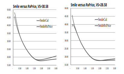
variance swap (within the class $\mathcal{M}^{c}$ ) in terms of a log-contract. A discretemonitoring variance swap pays at a maturity $T$ the sum of daily squared log-returns, mainly $$ \frac{1}{T} \sum_{i=0}^{n-1}\left(\ln \frac{S_{t_{i+1}}}{S_{t_{i}}}\right)^{2}, \quad t_{0}=0, \quad t_{n}=T $$ and $\Delta t=t_{i+1}-t_{i}=$ one day. In the limit $n \rightarrow \infty$, it converges $\mathbb{P}$-almost surely to the quadratic variation $\langle\ln S\rangle_{T}$ of $\ln S$ : $$ \frac{1}{T} \sum_{i=0}^{n-1}\left(\ln \frac{S_{t_{i+1}}}{S_{t_{i}}}\right)^{2} \stackrel{n \rightarrow \infty}{\longrightarrow} \frac{1}{T}\langle\ln S\rangle_{T} $$ REMARK 3.1 Note that in practice, $t_{k+1}-t_{k}=1$ day and the approximation of a discrete-monitored variance swap by its continuous-time version is valid. Indeed, $$ \mathrm{VS} \equiv \frac{1}{T} \sum_{i=0}^{n-1} \mathbb{E}\left[\left(\ln \frac{S_{t_{i+1}}}{S_{t_{i}}}\right)^{2}\right]=\frac{1}{T} \sum_{i=0}^{n-1} \mathbb{E}\left[\left(-\frac{1}{2}\left(\sigma_{t_{i}}^{\mathrm{LN}}\right)^{2} \Delta t+\sigma_{t_{i}}^{\mathrm{LN}} \Delta B_{t_{i}}\right)^{2}\right] $$ where $\sigma_{t_{i}}^{\mathrm{LN}}$ is the realized (log-normal) volatility between $\left[t_{i}, t_{i+1}\right], \Delta B_{t_{i}} \equiv$ $B_{t_{i+1}}-B_{t_{i}}$ and $T=n \Delta t$. This gives $$ \mathrm{VS} \equiv \frac{1}{T} \sum_{i=0}^{n-1} \mathbb{E}\left[\left(\frac{1}{4}\left(\sigma_{t_{i}}^{\mathrm{LN}}\right)^{4}(\Delta t)^{2}+\left(\sigma_{t_{i}}^{\mathrm{LN}}\right)^{2} \Delta t\right)\right] $$ By taking $\sigma_{t_{i}}^{\mathrm{LN}}=\sigma^{\mathrm{LN}}$ constant, we get $$ \sqrt{\mathrm{VS}} \equiv\left(\sigma^{\mathrm{LN}}\right)\left(1+\frac{1}{4}\left(\sigma^{\mathrm{LN}}\right)^{2} \Delta t\right)^{\frac{1}{2}} $$ If we impose a relative error of $10^{-3}$ between the continuous and the discrete version, we obtain $\Delta t=810^{-3} /\left(\sigma^{\mathrm{LN}}\right)^{2}$. For $\sigma^{\mathrm{LN}} \sim 100 \%$, we get $\Delta t \approx 3$ days.
统计代写|离散时间鞅理论代写martingale代考|Covariance options
We consider two liquid European options with payoffs $F_{1}$ and $F_{2}$ and maturity $T$, possibly depending on different assets. We denote $\mathbb{E}{t}^{\mathbb{P}}\left[F{1}\right]$ (resp. $\mathbb{E}{t}^{\mathbb{P}}\left[F{2}\right]$ ) the $t$-value of this option quoted on the market. The market uses a priori two (different) risk-neutral probability measures $\mathbb{P}^{1}$ and $\mathbb{P}^{2}$. We will assume
that they coincide and belong to $\mathcal{M}^{c}$. $\mathbb{P}$ is not known, we have only a partial characterization through the values $\mathbb{E}{t}^{\mathbb{P}}\left[F{1}\right]$ and $\mathbb{E}{t}^{\mathbb{P}}\left[F{2}\right]$. We assume also that the payoff $F_{1} F_{2}$ with maturity $T$ can be bought at $t=0$ with market prices $\mathbb{E}^{\mu}\left[F_{1} F_{2}\right]$
A covariance option pays at a maturity $T$ the daily realized covariance between the prices $\mathbb{E}{t}^{\mathbb{P}}\left[F{1}\right]$ and $\mathbb{E}{t}^{\mathbb{P}}\left[F{2}\right]$ : $$ \sum_{i=0}^{n-1}\left(\mathbb{E}{t{i+1}}^{\mathbb{P}}\left[F_{1}\right]-\mathbb{E}{t{i}}^{\mathbb{P}}\left[F_{1}\right]\right)\left(\mathbb{E}{t{i+1}}^{P}\left[F_{2}\right]-\mathbb{E}{t{i}}^{\mathbb{P}}\left[F_{2}\right]\right) $$ In the limit $n \rightarrow \infty$, it converges to $$ \int_{0}^{T} d\left\langle\mathbb{E}^{\mathbb{P}}\left[F_{1}\right], \mathbb{E}^{\mathbb{P}}\left[F_{2}\right]\right\rangle_{t} $$ From Itô’s lemma, we have for all $\mathbb{P} \in \mathcal{M}^{c}$ : $$ \begin{array}{r} \int_{0}^{T} d\left\langle\mathbb{E}^{\mathrm{P}}\left[F_{1}\right], \mathbb{E}^{\mathrm{P}}\left[F_{2}\right]\right\rangle_{t}=\left(F_{1} F_{2}-\mathbb{E}^{\mu}\left[F_{1} F_{2}\right]\right) \ +\left(\mathbb{E}^{\mu}\left[F_{1} F_{2}\right]-\mathbb{E}{0}^{\mathbb{P}}\left[F{1}\right] \mathbb{E}{0}^{\mathbb{P}}\left[F{2}\right]\right) \ -\int_{0}^{T} \mathbb{E}{t}^{\mathbb{P}}\left[F{1}\right] d \mathbb{E}{t}^{\mathbb{P}}\left[F{2}\right]-\int_{0}^{T} \mathbb{E}{t}^{\mathbb{P}}\left[F{2}\right] d \mathbb{E}{t}^{\mathbb{P}}\left[F{1}\right] \end{array} $$ As observed in $[76]$, this equality indicates that a covariance option can be replicated by doing a delta-hedging on $\mathbb{E}{t}^{\mathbb{P}}\left[F{1}\right]$ (resp. $\mathbb{E}{t}^{\mathbb{P}}\left[F{2}\right]$ ) with $H_{t}^{1} \equiv$ $-\mathbb{E}{t}^{\mathbb{P}}\left[F{2}\right]$ (resp. $H_{t}^{2} \equiv-\mathbb{E}{t}^{\mathrm{P}}\left[F{1}\right]$ ) and statically holding the $T$-European payoff $F_{1} F_{2}$ with market price $\mathbb{E}^{\mu}\left[F_{1} F_{2}\right]$. The model-independent price of this option is therefore $$ \begin{aligned} \mathbb{E}^{\mathbb{P}}\left[\int_{0}^{T} d\left\langle\mathbb{E}^{\mathbb{P}}\left[F_{1}\right], \mathbb{E}^{\mathbb{P}}\left[F_{2}\right]\right\rangle_{t}\right]=& \mathbb{E}^{\mu}\left[F_{1} F_{2}\right]-\mathbb{E}{0}^{\mathbb{P}}\left[F{1}\right] \mathbb{E}{0}^{\mathbb{P}}\left[F{2}\right] \ & \forall \mathbb{P} \in \mathcal{M}^{c} \cap\left{\mathbb{P}: \mathbb{E}^{\mathbb{P}}\left[F_{1} F_{2}\right]=\mathbb{E}^{\mu}\left[F_{1} F_{2}\right]\right} \end{aligned} $$
The enormous development of OT in the last decades was initiated by Brenier’s celebrated theorem, briefly reviewed in Theorem 2.3. Hence a most natural question is to obtain similar results also for the martingale version of the transport problem. The literature on this topic includes [82, 83]. This seems a potentially very interesting problem for mathematicians working in OT to tackle this problem, particularly in $\mathbb{R}^{d}$.
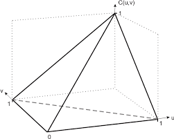
We briefly state below MOT in $\mathbb{R}{+}^{d}$. We denote $\mathbb{P}^{1}$ and $\mathbb{P}^{2}$ the marginals of $S{1}$ and $S_{2}$ in $\mathbb{R}{+}^{d}$ and $S{1}^{i}$ the $i$-component of $S_{1}$. The knowledge of marginals $\mathbb{P}^{1}$ and $\mathbb{P}^{2}$ is not very common in finance as the (known) marginals are usually one-dimensional (e.g. Vanillas), see however our discussion in Section 2.1.3. A notable exception arises in fixed income and foreign exchange markets (see Example 2.1) where Vanillas on spread swap rates, i.e., $\left(S_{2}-K S_{1}\right)^{+}$, are quoted on the market. MOT reads $$ \widetilde{\mathrm{MK}}{2}=\inf {\lambda_{1} \in \mathrm{L}^{1}\left(\mathbb{P}^{1}\right), \lambda_{2} \in \mathrm{L}^{1}\left(\mathbb{P}^{2}\right),\left(H^{i}(-)\right){1 \leq i \leq d}} \mathbb{E}^{\mathbb{P}^{1}}\left[\lambda{1}\left(S_{1}\right)\right]+\mathbb{E}^{\mathbb{P}^{2}}\left[\lambda_{2}\left(S_{2}\right)\right] $$ such that $\lambda_{1}\left(s_{1}\right)+\lambda_{2}\left(s_{2}\right)+\sum_{i=1}^{d} H^{i}\left(s_{1}\right)\left(s_{2}^{i}-s_{1}^{i}\right) \geq c\left(s_{1}, s_{2}\right), \quad \forall\left(s_{1}, s_{2}\right) \in$ $\left(\mathbb{R}{+}^{d}\right)^{2}$. Taking for granted that the primal is attained (the dual is attained by weak compactness), the (strong) duality result implies as before that $$ \lambda{1}\left(s_{1}\right)+\lambda_{2}\left(s_{2}\right)+\sum_{i=1}^{d} H^{i}\left(s_{1}\right)\left(s_{2}^{i}-s_{1}^{i}\right)=c\left(s_{1}, s_{2}\right), \quad \mathbb{P}^{}-\text { a.s. } $$ We have $d+2$ unknown functions $\left(\lambda_{1}, \lambda_{2},\left(H^{i}(\cdot)\right){1 \leq i \leq d}\right.$ ) (defined on (a subset of) $\mathbb{R}{+}^{d}$ ) and it is tempting to guess that the optimal martingale measure $\mathbb{P}^{}$ is localized on some maps $\left(T^{\alpha}\right){\alpha=1, \ldots, N}$. For each map – denoted schematically by $T$ with components $\left(T{1}, \ldots, T_{d}\right)$ – we should have: $\forall s_{1} \in \mathbb{R}^{d}$, $$ \begin{aligned} &\lambda_{1}\left(s_{1}\right)+\lambda_{2}\left(T\left(s_{1}\right)\right)+\sum_{i=1}^{d} H^{i}\left(s_{1}\right)\left(T_{i}\left(s_{1}\right)-s_{1}^{i}\right)=c\left(s_{1}, T\left(s_{1}\right)\right) \ &\partial_{s_{2}^{i}} \lambda_{2}\left(T\left(s_{1}\right)\right)+H^{i}\left(s_{1}\right)=\partial_{s_{2}^{i}} c\left(s_{1}, T\left(s_{1}\right)\right), \quad \forall i=1, \ldots, d \end{aligned} $$ On the dual side, we should have : $$ \mathbb{P}^{*}\left(d s_{1}, s_{2}\right)=\sum_{\alpha=1}^{N} q_{\alpha}\left(s_{1}\right) \delta_{T a\left(s_{1}\right)}\left(d s_{2}\right) \mathbb{P}^{1}\left(d s_{1}\right) $$ where the functions $\left(q_{\alpha}\right){\alpha=1, \ldots, N}$ are constrained by the algebraic equations: $$ \sum{\alpha=1}^{N} q_{\alpha}\left(s_{1}\right)=1, \quad \sum_{\alpha=1}^{N} q_{\alpha}\left(s_{1}\right)\left(T^{\alpha}\left(s_{1}\right)-s_{1}\right)=0 $$
统计代写|离散时间鞅理论代写martingale代考|Mirror coupling: The right-monotone martingale transport plan
Suppose that $c_{s_{1} s_{2} s_{2}}<0$. Then, the upper bound $\widetilde{\mathrm{MK}}{2}$ is attained by the right-monotone martingale transport map $$ \begin{array}{r} \mathbb{P}{*}\left(d s_{1}, d s_{2}\right)=\mathbb{P}^{1}\left(d s_{1}\right)\left(q\left(s_{1}\right) \delta_{\bar{T}{u}\left(s{1}\right)}\left(d s_{2}\right)+\left(1-q\left(s_{1}\right)\right) \delta_{\bar{T}{d}\left(s{1}\right)}\left(d s_{2}\right)\right) \ q(x)=\frac{x-\bar{T}{d}(x)}{\bar{T}{u}(x)-\bar{T}{d}(x)} \end{array} $$ where $\left(\bar{T}{d}, \bar{T}{u}\right)$ is defined as in $(2.31,2.32)$ with the pair of probability measures $\left(\overline{\mathrm{P}}^{1}, \overline{\mathrm{P}}^{2}\right):$ $$ \bar{F}^{1}\left(s{1}\right) \equiv 1-F^{1}\left(-s_{1}\right), \text { and } \bar{F}^{2}\left(s_{2}\right) \equiv 1-F^{2}\left(-s_{2}\right) . $$ To see this, we rewrite the OT problem equivalently with modified inputs: $$ \begin{aligned} \bar{c}\left(s_{1}, s_{2}\right) \equiv c\left(-s_{1},-s_{2}\right), & \overline{\mathbb{P}}^{1}\left(\left(-\infty, s_{1}\right]\right) \equiv \mathbb{P}^{1}\left(\left[-s_{1}, \infty\right)\right) \ \overline{\mathbb{P}}^{2}\left(\left(-\infty, s_{2}\right]\right) \equiv \mathbb{P}^{2}\left(\left[-s_{2}, \infty\right)\right) \end{aligned} $$ so that $\bar{c}{s{1} s_{2} s_{2}}>0$, as required in Theorem 2.8. Note that the martingale constraint is preserved by the map $\left(s_{1}, s_{2}\right) \mapsto\left(-s_{1},-s_{2}\right)$ (and not by our parity transformation $\left(s_{1}, s_{2}\right) \mapsto\left(s_{1},-s_{2}\right)$ in OT $)$.
Suppose that $c_{s_{1} s_{2} s_{2}}>0$. Then, the lower bound problem is explicitly solved by the right-monotone martingale transport plan. Indeed, it follows from the first part of the present remark that: $$ \begin{aligned} \inf {\mathbb{P} \in \mathcal{M}\left(\mathbb{P}^{1}, \mathbb{P}^{2}\right)} \mathbb{E}^{\mathbb{P}}\left[c\left(S{1}, S_{2}\right)\right] &=-\sup {\mathbb{P} \in \mathcal{M}\left(\mathbb{P}^{1}, \mathbb{P}^{2}\right)} \mathbb{E}^{\mathbb{P}}\left[-c\left(S{1}, S_{2}\right)\right] \ &=-\sup {\mathbb{P} \in \mathcal{M}\left(\mathbb{P}^{1}, \mathbb{R}^{2}\right)} \mathbb{E}^{\mathbb{P}}\left[-\bar{c}\left(-S{1},-S_{2}\right)\right] \ &=-\sup {\mathbb{P} \in \mathcal{M}\left(\mathbb{P}^{1}, \mathbb{R}^{2}\right)} \mathbb{E}^{\mathbb{P}}\left[-\bar{c}\left(S{1}, S_{2}\right)\right] \ &=\mathbb{E}^{\mathbb{P}}\left[c\left(S_{1}, S_{2}\right)\right] \end{aligned} $$
统计代写|离散时间鞅理论代写martingale代考|Change of num´eraire
We define the involution $\mathcal{S}[34]$ (i.e., $\mathcal{S}^{2}=\mathrm{Id}$ ) on a payoff function $c$ by $$ (\mathcal{S c})\left(s_{1}, s_{2}\right) \equiv s_{2} c\left(\frac{1}{s_{1}}, \frac{1}{s_{2}}\right) $$ We have $$ \begin{aligned} \sup {\mathbb{P} \in \mathcal{M}\left(\mathbb{P}^{1}, \mathbb{P}^{2}\right)} \mathbb{E}^{\mathbb{P}}\left[(\mathcal{S} c)\left(S{1}, S_{2}\right)\right]=& \sup {\mathbb{P} \in \mathcal{M}\left(\mathbb{P}^{1}, \mathbb{P}^{2}\right)} \mathbb{E}^{\mathbb{P}}\left[S{2} c\left(\frac{1}{S_{1}}, \frac{1}{S_{2}}\right)\right] \ =S_{0} & \sup {\left.\mathbb{Q} \in \mathcal{M}\left(\mathcal{S}^{1}\right), \mathcal{P}\left(\mathbb{(}^{2}\right)\right)} \mathbb{E}^{\mathbb{Q}}\left[c\left(\bar{S}{t_{1}}, \bar{S}{t{2}}\right)\right] \end{aligned} $$ where $\mathcal{S}\left(\mathbb{P}^{i}\right), i=1,2$ has a density $\left(\mathcal{S} f^{i}\right)(s)=\frac{1}{S_{0} s^{3}} f^{i}\left(\frac{1}{s}\right)$ where $f^{i}$ the density of $\mathbb{P}^{i}$. We have used that by working in the numéraire associated to the discrete martingale $S_{t}$ : $$ \mathbb{E}^{\mathrm{P}}\left[S_{2} c\left(\frac{1}{S_{1}}, \frac{1}{S_{2}}\right)\right]=S_{0} \mathbb{E}^{\mathbb{Q}}\left[c\left(\frac{1}{S_{1}}, \frac{1}{S_{2}}\right)\right] $$ with $\left.\frac{d \mathbb{Q}}{}\right|{\mathcal{F}{t_{i}}}=\frac{S_{i}}{S_{0}}$. Under $\mathbb{Q}, \frac{1}{S_{i}}$ is a discrete martingale: $\mathbb{E}^{\mathbb{Q}}\left[\frac{1}{S_{2}} \mid \frac{1}{S_{1}}\right]=\frac{1}{S_{1}}$. This involution $\mathcal{S}$ satisfies $$ (\mathcal{S c}){122}\left(s{1}, s_{2}\right)=-\frac{1}{s_{1}^{2} s_{2}^{3}} c_{122}\left(\frac{1}{s_{1}}, \frac{1}{s_{2}}\right) $$ and exchanges therefore the left and right-monotone martingale transport plan where the marginals have support in $\mathbb{R}_{+}$.
统计代写|离散时间鞅理论代写martingale代考|OT versus MOT: A summary
统计代写|离散时间鞅理论代写martingale代考|Multi-marginals and infinitely-many marginals case
Most of the literature on OT focuses on the 2 -asset case with a payoff $c\left(s_{1}, s_{2}\right)$. For applications in mathematical finance, it is interesting to study the case of a multi-asset payoff $c\left(s_{1}, \ldots, s_{n}\right)$ depending on $n$ assets evaluated at the same maturity. We define the $n$-asset optimal transport problem (by duality) as $$ \mathrm{MK}{n} \equiv \sup {\mathbb{P} \in \mathcal{P}\left(\mathbb{P}^{1}, \ldots, \mathbb{P}^{n}\right)} \mathbb{E}^{\mathbb{P}}\left[c\left(S_{1}, \ldots, S_{n}\right)\right] $$ with $\mathcal{P}\left(\mathbb{P}^{1}, \ldots, \mathbb{P}^{n}\right)=\left{\mathbb{P}: S_{i} \stackrel{\mathbb{P}}{\sim} \mathbb{P}^{i}, \forall i=1, \ldots, n\right}$. This problem has been studied by Gangbo [78] and recently by Carlier [36] (see also Pass [124]) with the following requirement on the payoff:
DEFINITION $2.4$ see [36] $c \in C^{2}$ is strictly monotone of order 2 if for all $(i, j) \in{1, \ldots, n}^{2}$ with $i \neq j$, all second order derivatives $\partial_{i j} c$ are positive. We have
THEOREM $2.4$ see $[78,36]$ If $c$ is strictly monotone of order 2 , there exists a unique optimal transference plan for the $\mathrm{MK}{n}$ transport problem, and it has the form $$ \mathbb{P}^{*}\left(d s{1}, \ldots, d s_{n}\right)=\mathbb{P}^{1}\left(d s_{1}\right) \prod_{i=2}^{n} \delta_{T_{i}\left(s_{1}\right)}\left(d s_{i}\right), \quad T_{i}(s)=F_{i}^{-1} \circ F_{1}(s), i=2, \ldots, n $$ The optimal upper bound is $$ \mathrm{MK}{n}=\int c\left(x, T{2}(x), \ldots, T_{n}(x)\right) \mathbb{P}^{1}(d x) $$ An extension to the infinite many marginals case has been obtained recently by Pass $[125]$ who studies $$ \mathrm{MK}{\infty} \equiv \sup {\mathbb{P}: S_{\mathrm{t}} \sim \mathbb{P} t, \forall t \in(0, T]} \mathbb{E}\left[h\left(\int_{0}^{T} S_{t} d t\right)\right] $$ where $h$ is a convex function. Let $F_{t}$ the cumulative distribution of $\mathbb{P}^{t}$. Define the stochastic process $S_{t}^{\text {opt }}(\omega)=F_{t}^{-1}(\omega), \quad \omega \in[0,1]$. The underlying probability space is the interval $[0,1]$ with Lebesgue measure.
统计代写|离散时间鞅理论代写martingale代考|Link with Hamilton-Jacobi equation
Here we take a cost function $c\left(s_{1}, s_{2}\right)=L\left(s_{2}-s_{1}\right)$ with $L$ a strictly concave function such that the Spence-Mirrlees condition is satisfied. From the formulation (2.8), one can link the Monge-Kantorovich formulation to the solution of a Hamilton-Jacobi equation through the Hopf-Lax formula: PROPOSITION 2.3 see e.g. [139] $$ \mathrm{MK}{2}=\inf {u(1, \cdot)}-\mathbb{E}^{\mathbb{P}^{1}}\left[u\left(0, S_{1}\right)\right]+\mathbb{E}^{\mathbb{P}^{2}}\left[u\left(1, S_{2}\right)\right] $$ where $u(0, \cdot)$ is the (viscosity) solution at $t=0$ of the following HJ equation with terminal boundary condition $u(1,-):$ $$ \partial_{t} u+H(D u)=0, \quad H(p) \equiv \inf _{q}{p q-L(q)} $$
PROOF From the dynamic programming principle, $u$, satisfying HamiltonJacobi equation (2.21), can be written as $$ u(t, x)=\inf {\zeta} u\left(1, x+\int{t}^{1} \dot{\zeta}(s) d s\right)-\int_{t}^{1} L(\dot{\zeta}(s)) d s $$ The minimisation over $\dot{\zeta}$ gives that $\dot{\zeta}$ is a constant $q$ (Fréchet derivative with respect to $\dot{\zeta}$ gives the critical equation $\left.\frac{d^{2} \zeta(t)}{d t^{2}}=0\right)$. $$ u(t, x)=\inf {q} u(1, x+q(1-t))-L(q)(1-t) $$ By setting $y=x+q(1-t)$, we get Hopf-Lax’s formula: $$ u(t, x)=\inf {y} u(1, y)-L\left(\frac{y-x}{1-t}\right)(1-t) $$ For $t=0$, this gives that $-u(0, \cdot)$ is the L-transform of $u(1, \cdot):-u(0, x)=$ $\sup _{y} L(y-x)-u(1, y)$. We conclude with Proposition 2.1.
In the next section, we introduce a martingale version of OT, first developed in $[17,77]$ where we have obtained a Monge-Kantorovich duality result.
统计代写|离散时间鞅理论代写martingale代考|Martingale optimal transport
We consider a payoff $c\left(s_{1}, s_{2}\right)$ depending on a single asset evaluated at two dates $t_{1}{2}$ : DEFINITION $2.5$ $$ \widetilde{\mathrm{MK}}{2} \equiv \inf {\mathcal{M}^{}\left(\mathbb{P}^{1}, \mathbb{P}^{2}\right)} \mathbb{E}^{\mathbb{P}^{1}}\left[\lambda{1}\left(S_{1}\right)\right]+\mathbb{E}^{\mathbb{P}^{2}}\left[\lambda_{2}\left(S_{2}\right)\right] $$ where $\mathcal{M}^{}\left(\mathbb{P}^{1}, \mathbb{P}^{2}\right)$ is the set of functions $\lambda_{1} \in \mathrm{L}^{1}\left(\mathbb{P}^{1}\right), \lambda_{2} \in \mathrm{L}^{1}\left(\mathbb{P}^{2}\right)$ and $H$ a bounded continuous function on $\mathbb{R}{+}$such that $$ \lambda{1}\left(s_{1}\right)+\lambda_{2}\left(s_{2}\right)+H\left(s_{1}\right)\left(s_{2}-s_{1}\right) \geq c\left(s_{1}, s_{2}\right), \quad \forall\left(s_{1}, s_{2}\right) \in \mathbb{R}{+}^{2} $$ This corresponds to a semi-static hedging strategy which consists in holding European payoffs $\lambda{1}$ and $\lambda_{2}$ and applying a delta strategy at $t_{1}$, generating a
$\mathrm{P} \& \mathrm{~L} H\left(s_{1}\right)\left(s_{2}-s_{1}\right)$ at $t_{2}$ with zero cost. We could also add a term $H_{0}\left(S_{0}\right)\left(s_{1}-\right.$ $\left.S_{0}\right)$ corresponding to performing a delta-hedging at $t=0$. As this term can be incorporated into $\lambda_{1}\left(s_{1}\right)$, it is not included. Similarly, an intermediate deltahedging term $H_{i}\left(S_{0}, \ldots, s_{t_{i}}\right)\left(s_{t_{i+1}}-s_{t_{i}}\right)$ where $0<t_{i}<t_{i+1} \leq t_{2}$ can be added but it can be shown that the optimal solution is attained for $H_{i}=0$. These terms are therefore not needed and will be disregarded next (see Corollary $2.1)$
Note that in comparison with the OT MK $\mathrm{MK}{2}$ previously reported, we have $\overline{\mathrm{MK}}{2} \leq \mathrm{MK}_{2}$ due to the appearance of the function $H$.
At this point, a natural question is how the classical results in OT generalize in the present martingale version. We follow closely our introduction of OT and explain how the various concepts previously explained extend to the present setting. Our research partly originates from a systematic derivation of Skorokhod embedding solutions and understanding of particle methods for non-linear McKean stochastic differential equations appearing in the calibration of financial models (see Section 4.2.4). From a practical point of view, the derivation of these optimal bounds allows to better understand the risk of exotic options as illustrated in the next example.
统计代写|离散时间鞅理论代写martingale代考|Derivation of the Monge–Amp`ere equation
统计代写|离散时间鞅理论代写martingale代考|Axiomatic construction of marginals: Stieltjes moment problem
We have explained previously that marginals $\mathbb{P}^{i}$ can be inferred from market values of $T$-Vanilla call/put options. However, in practice, only a finite number of strikes are quoted and therefore these liquid prices need to be interpolated and extrapolated in order to imply the marginals $\mathbb{P}^{i}$ (supported in $\mathbb{R}{+}$). We report here how this can be achieved. This problem can be framed as Stieltjes moment problem. By construction, our $T$-marginal should belong to the infinite-dimensional convex set $$ \mathcal{M}=\left{\mathbb{P}: \mathbb{E}^{\mathbb{P}}\left[S{T}\right]=S_{0}, \quad \mathbb{E}^{\mathbb{P}}\left[\left(S_{T}-K_{i}\right)^{+}\right]=C\left(K_{i}\right) \equiv c_{i}, \quad i=1, \ldots n\right} $$ $\mathcal{M}$ is relatively compact from Prokhorov’s theorem (See Remark 1.4). For instance, we add the technical assumption that the elements in $\mathcal{M}$ should also be compactly supported in the interval $\left[0, S_{\max }\right]$ with $S_{\max }$ large in order to get that $\mathcal{M}$ is compact. This implies that from Krein-Milman’s theorem, this set can be reconstructed from its extremal points $\operatorname{Ext}(\mathcal{M})$ : $$ \mathcal{M}=\overline{\operatorname{Conv}(\operatorname{Ext}(\mathcal{M}))} $$ Furthermore, from Choquet’s theorem, one can show that all arbitrage-free prices $C(K)$ can be obtained by linearly combining extremal points. They are supported by a probability measure $\mu$ on $\operatorname{Ext}(\mathcal{M})$ (probability on probability space!) and for all $K$, $$ C(K)=\int_{\operatorname{Ext}(\mathcal{M})} \mathbb{E}^{\mathbb{P}}\left[\left(S_{T}-K\right)^{+}\right] d \mu(\mathbb{P}) $$ Enumerating all the extremal points (and therefore elements in $\mathcal{M}$ ) is a difficult task. We follow a different route. A canonical point of $\mathcal{M}$ can be obtained by minimising a convex lower semi-continuous functional $\mathcal{F}$ : $$ I \equiv \inf {\mathbb{P} \in \mathcal{M}} \mathcal{F}(\mathbb{P})=\mathcal{F}\left(\mathbb{P}{c_{1}, \ldots, c_{n}}^{}\right), \quad \mathbb{P}{c{1}, \ldots, c_{n}}^{} \in \mathcal{M} $$
The Spence-Mirrlees condition, i.e., $c_{12}>0$, required for the Fréchet-Hoeffding solution to hold, is very natural from a financial point of view. If we shift the payoff $c$ by some European payoffs $\Lambda_{1} \in L^{1}\left(\mathbb{P}^{1}\right), \Lambda_{2} \in L^{1}\left(\mathbb{P}^{2}\right)$ : $$ \bar{c}\left(s_{1}, s_{2}\right)=c\left(s_{1}, s_{2}\right)+\Lambda_{1}\left(s_{1}\right)+\Lambda_{2}\left(s_{2}\right) $$ then the Monge-Kantorovich bound for $\bar{c}$ should be $$ \mathrm{MK}{2}(\bar{c})=\mathrm{MK}{2}(c)+\mathbb{E}^{\mathbb{P}^{1}}\left[\Lambda_{1}\left(S_{1}\right)\right]+\mathbb{E}^{\mathbb{P}^{2}}\left[\Lambda_{2}\left(S_{2}\right)\right] $$ as the market price of $\Lambda_{i}\left(s_{i}\right)$ is fixed by $\mathbb{E}^{\mathbb{P}^{x}}\left[\Lambda_{i}\left(S_{i}\right)\right]$. The payoff $\bar{c}$ is precisely invariant under the Spence-Mirrlees condition : $\bar{c}{12}=c{12}$.
Similarly, the upper bound under the condition $c_{12}<0$ is attained by the co-monotone rearrangement map $$ T\left(s_{1}\right)=F_{2}^{-1} \circ\left(1-F_{1}\left(-s_{1}\right)\right) $$ This can be obtained by applying the parity transformation $\mathcal{P}\left(s_{1}, s_{2}\right)=$ $\left(-s_{1}, s_{2}\right)$. For each measure $\mathbb{P}$ matching the marginals $\mathbb{P}^{1}$ and $\mathbb{P}^{2}$, we can associate the measure $\mathcal{P}{} \mathbb{P}$ matching the marginals $\mathcal{P}{} \mathbb{P}^{1}$ and $\mathbb{P}^{2}$ with cumulative distributions $\bar{F}{1}\left(s{1}\right) \equiv 1-F_{1}\left(-s_{1}\right)$ and $F_{2}\left(s_{2}\right)$. We conclude as the Monge-Kantorovich bounds for $c$ and $\tilde{c}\left(s_{1}, s_{2}\right) \equiv c\left(-s_{1}, s_{2}\right)$ coincides as $\mathbb{E}^{\mathbb{P}}[c]=\mathbb{E}^{\mathcal{P}} \mathbb{P}[\bar{c}]$. Similarly, by replacing $c$ by $-c$, we obtain that the comonotone rearrangement map gives the lower bound under the condition $c_{12}>0$ Example $2.4$ Lower bound, $c\left(s_{1}, s_{2}\right)=\left(s_{1}-K_{1}\right)+1_{s_{2}>K_{2}}$ By applying Anti-Fréchet-Hoeffding solution, the lower bound is attained by $$ \mathrm{MK}{2}=\int{F_{2}\left(K_{2}\right)}^{\max \left(1-F_{1}\left(K_{1}\right), F_{2}\left(K_{2}\right)\right)}\left(F_{1}^{-1}(1-u)-K_{1}\right) d u $$ with $$ \begin{aligned} &\lambda_{2}(x)=\left(\bar{F}{1}^{-1} \circ F{2}\left(K_{2}\right)-K_{1}\right)^{+} 1_{x>K_{2}} \ &\lambda_{1}(x)=\left(x-K_{1}\right)^{+} 1_{F_{2}^{-1} \circ F_{1}(x)>K_{2}}-\left(\bar{F}{1}^{-1} \circ F{2}\left(K_{2}\right)-K_{1}\right)^{+} 1_{F_{2}^{-1} \circ F_{1}(x)>K_{2}} \end{aligned} $$
统计代写|离散时间鞅理论代写martingale代考|Derivation of the Monge–Amp`ere equation
统计代写|离散时间鞅理论代写martingale代考|Martingale optimal transport
统计代写|离散时间鞅理论代写martingale代考|Formulation in R+d and multi-dimensional marginals
The MK formulation and its dual expression remain valid when $S_{1}$ and $S_{2}$ are two random variables in $\mathbb{R}{+}^{d}$. The interpretation in mathematical finance goes as follows: let us consider a payoff $c\left(s{1}, s_{2}\right)$ depending on two groups $\left(s_{1}, s_{2}\right)$, each composed of $d$ assets. The first group is $\left(s_{1}^{1}, \ldots, s_{1}^{d}\right) \in \mathbb{R}{+}^{d}$. Knowing the distribution of $S{1} \in \mathbb{R}{+}^{d}$ is equivalent to knowing (at $t=0$ ) the market values of all basket options $\mathbb{E}^{\mathbb{P}^{1}}\left[\left(S{1} \cdot \omega-K\right)^{+}\right]$for all $K \in \mathbb{R}$ and for all $\omega \in \mathbb{R}^{d}$. This equivalence can be seen by observing that basket option prices fix the Laplace transform of $S_{1}: \mathbb{E}^{P^{1}}\left[e^{\omega-S_{1}}\right]$. Although basket options are liquid only for some particular values of the weight $\omega$ (and $K)$, the values $\mathbb{E}^{\mathbb{P}^{1}}\left[\left(S_{1} \cdot \omega-K\right)^{+}\right]$can be however fixed by assuming a correlation structure (more precisely a copula, denoted co below) between the variables $\left(S_{1}^{1}, \ldots, S_{1}^{d}\right)$. For example, the first group of assets (resp. second) belongs to the same financial sector and can therefore be assumed to be strongly correlated. This is not the case for the correlation structures between $S_{1}$ and $S_{2}$ which belong to two different groups and for which the correlation information is difficult to obtain. This is found through our OT formulation. By definition of the copula co, we impose that $$ \mathbb{E}^{\mathbb{P}^{1}}\left[\lambda_{1}\left(S_{1}\right)\right] \equiv \mathbb{E}\left[\lambda_{1}\left(F_{1}^{-1}\left(U_{1}\right), \ldots F_{d}^{-1}\left(U_{d}\right)\right) \operatorname{co}\left(U_{1}, \ldots, U_{d}\right)\right] $$ where $\left(U_{i}\right){1 \leq i \leq d}$ are $d$ independent uniform random variables and $F{i}$ is the cumulative distribution of $S_{1}^{i}$ implied from $T$-Vanilla options on $S_{1}^{i}$. Note that our discussion can be extended when $S_{1} \in \mathbb{R}{+}^{d}$ and $S{2} \in \mathbb{R}_{+}^{d^{}}$ with $d \neq d^{}$.
Under the so-called Spence-Mirrlees condition, $c_{12} \equiv \partial_{s_{1} s_{2}} c>0$, OT (2.6) can be solved explicitly. Let $F_{1}, F_{2}$ denote the cumulative distribution functions of $\mathbb{P}^{1}$ and $\mathbb{P}^{2}$. For the sake of simplicity, we will assume that $\mathbb{P}^{1}$ does not give mass to points and $c \in C^{2}$. THEOREM $2.2$ Under $c_{12}>0$, (i): The optimal measure $\mathbb{P}^{}$ has the form $$ \mathbb{P}^{}\left(d s_{1}, d s_{2}\right)=\delta_{T\left(s_{1}\right)}\left(d s_{2}\right) \mathbb{P}^{1}\left(d s_{1}\right) $$ with $T$ the forward image of the measure $\mathbb{P}^{1}$ onto $\mathbb{P}^{2}: T(x)=F_{2}^{-1} \circ F_{1}(x)$. (ii): The optimal upper bound is given by $$ \mathrm{MK}{2}=\int{0}^{1} c\left(F_{1}^{-1}(u), F_{2}^{-1}(u)\right) d u $$ This optimal bound can be attained by a static hedging strategy consisting in holding European payoffs $\lambda_{1} \in \mathrm{L}^{1}\left(\mathbb{P}^{1}\right), \lambda_{2} \in \mathrm{L}^{1}\left(\mathbb{P}^{2}\right)$ with market prices $\mathbb{E}^{\mathbb{P}^{1}}\left[\lambda_{1}\left(S_{1}\right)\right]$ and $\mathbb{E}^{\mathbb{P}^{2}}\left[\lambda_{2}\left(S_{2}\right)\right]$ $$ \mathrm{MK}{2}=\mathbb{E}^{\mathbb{P}^{1}}\left[\lambda{1}\left(S_{1}\right)\right]+\mathbb{E}^{\mathbb{P}^{2}}\left[\lambda_{2}\left(S_{2}\right)\right] $$ with $$ \lambda_{2}(x)=\int_{0}^{x} c_{2}\left(T^{-1}(y), y\right) d y, \quad \lambda_{1}(x)=c(x, T(x))-\lambda_{2}(T(x)) $$ The value of this static European portfolio super-replicates the payoff at maturity: $$ \lambda_{1}\left(s_{1}\right)+\lambda_{2}\left(s_{2}\right) \geq c\left(s_{1}, s_{2}\right), \quad \forall\left(s_{1}, s_{2}\right) \in \mathbb{R}{+}^{2} $$ $T$ is refereed as the Brenier map (or Fréchet-Hoeffding). Note that the above theorem requires additional conditions on $c$ in order to guarantee the integrability conditions $\lambda{1} \in L^{1}\left(\mathbb{P}^{1}\right)$ and $\lambda_{2} \in L^{1}\left(\mathbb{P}^{2}\right)$.
统计代写|离散时间鞅理论代写martingale代考|Brenier’s solution
The Fréchet-Hoeffding solution has been generalized in $\mathbb{R}^{d}$ by Brenier [29] first in the case of a quadratic cost function and then extended to concave payoff $c=c\left(s_{1}-s_{2}\right)$ by Gangbo and McCann $[79]$ and others: THEOREM 2.3 Brenier $=c\left(s_{1}, s_{2}\right)=-\left|s_{1}-s_{2}\right|^{2} / 2$ (i): If $\mathbb{P}^{1}$ has no atoms, then there is a unique optimal $\mathbb{P}^{}$, which is a Monge solution: $$ \mathbb{P}^{}=\delta_{T\left(s_{1}\right)}\left(d s_{2}\right) \mathbb{P}^{1}\left(s_{1}\right) $$ with $T=\nabla \lambda_{1} . \nabla \lambda_{1}$ is the unique gradient of a convex function $\lambda_{1}$. (ii): The optimal bound is attained by a static hedging strategy with $\lambda_{2}(x)=$ $c(x, T(x))-\lambda_{1}(x)$ and $\lambda_{1}$ uniquely specified by $$ \left(\nabla \lambda_{1}\right) # \mathbb{P}^{1}=\mathbb{P}^{2} $$ The notation $T # \mathbb{P}^{1}=\mathbb{P}^{2}$ means that for all $U \in \mathrm{L}^{1}\left(\mathbb{P}^{2}\right)$ : $$ \mathbb{E}^{\mathbb{P}^{1}}\left[U\left(T\left(S_{1}\right)\right)\right]=\mathbb{E}^{\mathbb{P}^{2}}\left[U\left(S_{2}\right)\right] $$ If $T$ is differentiable, this condition reads $$ |\operatorname{det} \nabla T| \mathbb{P}^{2}(T(x))=\mathbb{P}^{1}(x) $$
This theorem has been generalized to a strictly concave, superlinear ${ }^{2}$ cost function $c\left(s_{1}, s_{2}\right)=c\left(s_{1}-s_{2}\right)$. The Brenier map is then $$ T(x)=x-\nabla c^{}\left(\nabla \lambda_{1}(x)\right) $$ for some $c$-concave function $\lambda_{1}$ which is uniquely fixed by the requirement $T_{#} \mathbb{P}^{1}=\mathbb{P}^{2}$. Here $c^{} \equiv \inf _{x}{p . x-c(x)}$ is the Legendre transform of $c .$
统计代写|离散时间鞅理论代写martingale代考|Martingale optimal transport
Our delta-hedging strategy was a bit too simple as it consists only in buying or selling the asset at $t=0$ and holding it until the maturity. A more involved strategy is to buy (or sell) units of the asset at a date $t_{k}$ until a next date $t_{k+1}$. Let us compute the value of our delta-hedged portfolio at the maturity $T$. At $t_{k}$, the portfolio value $\pi_{t_{k}}$ is $$ \pi_{t_{k}}=\left(\pi_{t_{k}}-H_{t_{k}} S_{t_{k}}\right)+H_{t_{k}} S_{t_{k}} $$ where $H_{t_{k}}$ is the number of shares held at time $t_{k}$. Although this expression seems algebraically trivial, its financial interpretation is important: the term $H_{t_{k}} S_{t_{k}}$ is the value at $t_{k}$ of a position consisting of $H_{t_{k}}$ units of the asset. The term $\pi_{t_{k}}-H_{t_{k}} S_{t_{k}}$ represents the cash part invested in a bank account. The variation of our portfolio between $t_{k}$ and $t_{k+1}$ is then $$ \begin{aligned} \delta \pi_{t_{k}} &=\left(\pi_{t_{k}}-H_{t_{k}} S_{t_{k}}\right) r \delta t+H_{t_{k}} \delta S_{t_{k}} \ &=\pi_{t_{k}} r \delta t+H_{t_{k}}\left(\delta S_{t_{k}}-S_{t_{k}} r \delta t\right) \end{aligned} $$ with $\delta S_{t_{k}} \equiv S_{t_{k+1}}-S_{t_{k}}, \delta t=t_{k+1}-t_{k}$ small enough. As no cash is injected between $t_{k}$ and $t_{k+1}$, our portfolio is called self-financing. By setting $\bar{\pi}{t{k}} \equiv e^{-r t_{k}} \pi_{t_{k}}$ and $\bar{S}{t{k}} \equiv e^{-r t_{k}} S_{t_{k}}$, we obtain the variation of the discounted portfolio $$ \delta \tilde{\pi}{t{k}}=H_{t_{k}} \delta \tilde{S}{t{k},}, \delta \tilde{S}{t{k}} \equiv \tilde{S}{t{k+1}}-\tilde{S}{t{k}} $$ Here the state of information evolves over time and is described by a filtration $\mathcal{F}=\left(\mathcal{F}{t{1}}, \ldots, \mathcal{F}{t{n}}\right)$ where the $\sigma$-algebra $\mathcal{F}_{t}$ is the set of events that will be known to be true or false. We take here $\mathcal{F}{t{k}}=\sigma\left(S_{0}, \ldots, S_{t_{k}}\right)$ the natural filtration. $H_{k}=H_{k}\left(S_{0}, \ldots, S_{t_{k}}\right)$ is adapted, i.e., a measurable function with respect to $\mathcal{F}{t{k}}$ : we don’t look into the future. If we now assume that the trader sells an option with payoff $F_{T}$ at the price $C$ at $t=0$ and then delta-hedges his position at the intermediate dates $t_{0} \equiv 0<t_{1}<\ldots<t_{n} \equiv T$, we get $$ e^{-r T} \pi_{T}=-e^{-r T} F_{T}+C+\sum_{k=0}^{n-1} H_{t_{k}}\left(S_{0}, \ldots, S_{t_{k}}\right) \delta \bar{S}{t{k}} $$ By playing the same game as in Theorem 1.1, we obtain the dual expression:
Here we assume some familiarity with stochastic analysis. However, this section is not needed for the rest of the book and therefore can be skipped (see however the expression of the Black-Scholes formula). We consider that $S_{t}$ is modeled by a log-normal process under $\mathbb{P}^{\text {hist. }}$ : $$ \frac{d S_{t}}{S_{t}}=\mu d t+\sigma d W_{t}^{\mathrm{P}^{\text {hint }}} $$ $\mathcal{M}{\infty}$ corresponds to the set of $\mathbb{Q}$-martingale measure equivalent to Phist $^{\text {. From }}$ the Girsanov theorem (see e.g. $[130]), \mathcal{M}{\infty}$ reduces to a singleton $\left{\mathbb{Q}^{\mathrm{BS}}\right}$ under which $$ \frac{d S_{t}}{S_{t}}=r d t+\sigma d W_{t}^{\mathrm{Q}^{\mathrm{BS}}} $$ We conclude that there is a unique arbitrage-free price (independent of $\mu$ compare with formula (1.6)): $$ C=\mathbb{E}^{\mathrm{Q}^{\mathrm{BS}}}\left[e^{-r T} F_{T}\right] $$ We deduce also that the payoff can be dynamically hedged: $$ -e^{-r T} F_{T}+C+\int_{0}^{T} \partial_{S_{t}} \mathbb{E}^{\mathbb{Q}^{\mathrm{BS}}}\left[e^{-r(T-t)} F_{T} \mid S_{t}\right] d \tilde{S}{t}=0, \quad \text { Phist }^{-a . s .} $$ Note that for a call payoff $F{T}=\left(S_{T}-K\right)^{+}$, we obtain the Black-Scholes formula.
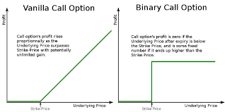
We assume that $T$-Vanilla options on each asset are traded on the market. They are specified by a payoff $\lambda\left(S_{T}\right)$ at a maturity $T$. In practice, these Vanilla payoffs can be replicated by holding a strip of put/call $T$-Vanillas through the Taylor expansion formula [38]: $$ \begin{aligned} \lambda\left(S_{T}\right)=\lambda\left(S_{0}\right)+\lambda^{\prime}\left(S_{0}\right)\left(S_{T}-S_{0}\right) &+\int_{0}^{S_{\mathrm{a}}} \lambda^{\prime \prime}(K)\left(K-S_{T}\right)^{+} d K \ &+\int_{S_{0}}^{\infty} \lambda^{\prime \prime}(K)\left(S_{T}-K\right)^{+} d K \end{aligned} $$ where $\left(K-S_{T}\right)^{+}\left(\right.$resp. $\left.\left(S_{T}-K\right)^{+}\right)$is the payoff of a put (resp. call). Derivatives $\lambda^{\prime \prime}(K)$ are understood in the distribution sense. We then assume that the pricing operator $\Pi[\cdot]$ (used by market operators to value Vanillas) is linear meaning that $$ \Pi\left[\sum_{i} \lambda_{i}\left(S_{T}-K_{i}\right)^{+}\right]=\sum_{i} \lambda_{i} \Pi\left[\left(S_{T}-K_{i}\right)^{+}\right] $$
Moreover, from the no-arbitrage condition, we should have that $$ \Pi[1]=e^{-r T}, \quad \Pi\left[S_{T}\right]=S_{0} $$ Also, still from the no-arbitrage condition, $\Pi\left[\left(S_{T}-K\right)^{+}\right]$should be nonincreasing, convex with respect to $K$ and $\Pi\left[\left(S_{T}-K\right)^{+}\right] \geq\left(S_{0}-K e^{-r T}\right)^{+}$. From Riesz’s representation theorem (with the additional requirement that the market price of a call option with strike $K$ goes to 0 as $K \rightarrow \infty$ ), this implies that there exists a probability $\mathbb{P}^{m k t}$ such that $$ C(K) \equiv \Pi\left[\left(S_{T}-K\right)^{+}\right]=\mathbb{E}^{\mathbb{P}^{\mathrm{mkt}}}\left[e^{-r T}\left(S_{T}-K\right)^{+}\right] $$ with $\mathbb{E}^{\text {prkt }}\left[e^{-r T} S_{T}\right]=S_{0}$. Below and in the rest of the book, for the sake of simplicity, we take $r=0$. This can be easily relaxed by including in the formulas below a multiplicative factor $e^{-r T}$.
From the linear property, the market price of the payoff $\lambda\left(S_{T}\right)$, inferred from market prices of put/call options, is $$ \begin{aligned} \Pi\left[\lambda\left(S_{T}\right)\right]=\mathbb{E}^{\mathrm{P}^{\mathrm{mkt}}}\left[\lambda\left(S_{T}\right)\right] &=\lambda\left(S_{0}\right)+\int_{0}^{S_{0}} \lambda^{\prime \prime}(K) \mathbb{E}^{\mathbb{P}^{\mathrm{mkt}}}\left[\left(K-S_{T}\right)^{+}\right] d K \ &+\int_{S_{0}}^{\infty} \lambda^{\prime \prime}(K) \mathbb{E}^{\mathrm{P}^{\mathrm{mkt}}}\left[\left(S_{T}-K\right)^{+}\right] d K \end{aligned} $$