标签: MATH 141

数学代写|微积分代写Calculus代写|MTH-211

如果你也在 怎样代写微积分Calculus 这个学科遇到相关的难题,请随时右上角联系我们的24/7代写客服。微积分Calculus 基本上就是非常高级的代数和几何。从某种意义上说,它甚至不是一门新学科——它采用代数和几何的普通规则,并对它们进行调整,以便它们可以用于更复杂的问题。(当然,问题在于,从另一种意义上说,这是一门新的、更困难的学科。)

微积分Calculus数学之所以有效,是因为曲线在局部是直的;换句话说,它们在微观层面上是直的。地球是圆的,但对我们来说,它看起来是平的,因为与地球的大小相比,我们在微观层面上。微积分之所以有用,是因为当你放大曲线,曲线变直时,你可以用正则代数和几何来处理它们。这种放大过程是通过极限数学来实现的。

statistics-lab™ 为您的留学生涯保驾护航 在代写微积分Calculus方面已经树立了自己的口碑, 保证靠谱, 高质且原创的统计Statistics代写服务。我们的专家在代写微积分Calculus代写方面经验极为丰富,各种代写微积分Calculus相关的作业也就用不着说。

数学代写|微积分代写Calculus代写|MTH-211

数学代写|微积分代写Calculus代写|ThE Growth OF KinEMatics IN thE WeST

Whereas in dynamics movement is studied in relation to the forces associated with it, in kinematics only its spatial and temporal aspects are considered. It follows that in kinematics we are concerned with the description of movement and not with its causes and it can therefore properly be regarded as the geometry of movement.

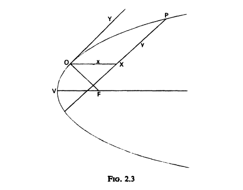
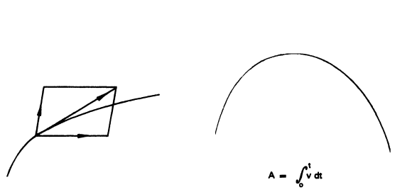
If a particle be known to trace a given curve the geometric properties of that curve can be used to predict the subsequent positions of the particle; conversely, if a curve be defined as the path of a point moving under specified conditions, then the laws of kinematics can be utilised to provide information as to certain geometric properties of the curve. For example, knowledge of the instantaneous motion at a given point on the curve enables us to draw the tangent to the curve at that point. The development, in the fourteenth century, of certain important concepts of motion including instantaneous velocity can therefore be seen to have direct and immediate bearing on the study of the tangent properties of curves. Furthermore, the introduction of graphical methods of representation led to the establishment of a link between the velocity-time graph, the total distance covered and the area under the curve, and this in turn is closely connected with the integral calculus (see Figs. 2.8 and 2.9).

The imaginative insights gained by the use of kinematic concepts in geometry were responsible for some of the more powerful methods developed during the seventeenth century for the study of curves. The work of Isaac Barrow, for instance, which certainly influenced Newton, is dominated by the idea of curves generated by moving points and lines.

数学代写|微积分代写Calculus代写|The Latitude OF Forms

At Merton College, Oxford, between the years 1328 and 1350, the distinction between kinematics and dynamics was made explicit. In the work of Thomas Bradwardine, William Heytesbury, Richard Swineshead and John Dumbleton the foundations for further study in this field were laid through the clarification and formalisation of a number of important concepts including the notion of instantaneous velocity (velocitas instantanea). ${ }^{\dagger}$

The study of space and motion at Merton College arose from the mediaeval discussion of the intension and remission of forms, i.e. the increase and decrease of the intensity of qualities. The distinction between intension and extension is exemplified in the case of heat by the difference between temperature, or degree of heat, and quantity of heat; in the case of weight between density, or weight per unit volume and total weight. For local motion the distinction is between velocity (or motion) at a given instant (instantaneous velocity) and total motion over a period of time, i.e. distance covered.

William Heytesbury distinguishes between uniform and difform (nonuniform) motion. In the case of difform motion he says: $\ddagger if, in a period of time, it were moved uniformly at the same degree of velocity (uniformiter illo gradu velocitatis) with which it is moved in that given instant, whatever [instant] be assigned.

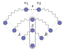
The most notable single achievement of the Merton School was the establishment of the mean speed theorem for uniformly accelerated (uniformly difform) motion, i.e. $s=\left(v_1+v_2\right) t / 2$, where $s$ is the distance covered in time $t$ and $v_1$ and $v_2$ are the initial and final velocities. Various proofs of this theorem were presented, some purely arithmetical and others depending on some skilful manipulation of infinite series. Although in some cases velocities (or intensions) were represented by single straight lines and Richard Swineshead actually uses a geometric analogy ${ }^{\dagger}$ to explain intension and remission of qualities it was not until knowledge of the Merton College work reached France and Italy that it received the full benefits of geometric representation and so linked kinematics with the geometry of straight and curved lines.

数学代写|微积分代写Calculus代写|MTH-211

微积分代考

数学代写|微积分代写Calculus代写|ThE Growth OF KinEMatics IN thE WeST

在动力学中,运动是根据与之相关的力来研究的,而在运动学中,只考虑其空间和时间方面。由此可见,在运动学中,我们所关心的是运动的描述,而不是运动的原因,因此,运动学可以恰当地看作是运动的几何学。

如果已知粒子沿给定曲线运动,则该曲线的几何特性可用于预测粒子的后续位置;相反,如果一条曲线被定义为一个点在特定条件下运动的路径,那么运动学定律可以用来提供关于曲线的某些几何性质的信息。例如,知道曲线上某一点的瞬时运动,我们就能画出该点与曲线的切线。因此,在14世纪,包括瞬时速度在内的某些重要运动概念的发展,可以看作对曲线的切线性质的研究有直接和直接的影响。此外,图形表示方法的引入使速度-时间图、覆盖的总距离和曲线下的面积之间建立了联系,而这又与积分学密切相关(见图2.8和图2.9)。

利用几何学中的运动学概念所获得的富有想象力的洞见,促成了17世纪研究曲线的一些更有力的方法的发展。例如,艾萨克·巴罗(Isaac Barrow)的工作,当然影响了牛顿,主要是由移动的点和线产生曲线的想法。

数学代写|微积分代写Calculus代写|The Latitude OF Forms

1328年至1350年间,牛津大学默顿学院明确区分了运动学和动力学。在Thomas Bradwardine, William Heytesbury, Richard Swineshead和John Dumbleton的工作中,通过澄清和形式化一些重要的概念,包括瞬时速度(velocitas instantanea)的概念,为该领域的进一步研究奠定了基础。${} ^{\匕首}$

默顿学院对空间和运动的研究源于中世纪对形式的强度和缓解的讨论,即质量强度的增加和减少。在热的情况下,强度和延伸之间的区别可以通过温度或热度与热量之间的差异来举例说明;在密度或单位体积重量与总重量之间的情况下。对于局部运动,区别在于给定瞬间(瞬时速度)的速度(或运动)和一段时间内的总运动,即所走过的距离。

威廉·海茨伯里区分了均匀运动和非均匀运动。在不均匀运动的情况下,他说:“如果在一段时间内,物体以与它在给定瞬间的运动速度相同的速度均匀运动,无论给定的是什么。”

默顿学派最著名的成就是建立了均匀加速(均匀均匀)运动的平均速度定理,即$s=\左(v_1+v_2\右)t / 2$,其中$s$是时间所覆盖的距离$t$, $v_1$和$v_2$是初始和最终速度。给出了这个定理的各种证明,有些是纯粹的算术证明,有些则依赖于对无穷级数的一些巧妙的处理。虽然在某些情况下,速度(或强度)是用一条直线来表示的,Richard Swineshead实际上使用了一个几何类比来解释强度和质量的缓解,但直到默顿学院的研究成果传播到法国和意大利,它才充分受益于几何表示,并将运动学与直线和曲线的几何联系起来。

数学代写|微积分代写Calculus代写 请认准statistics-lab™

统计代写请认准statistics-lab™. statistics-lab™为您的留学生涯保驾护航。

微观经济学代写

微观经济学是主流经济学的一个分支,研究个人和企业在做出有关稀缺资源分配的决策时的行为以及这些个人和企业之间的相互作用。my-assignmentexpert™ 为您的留学生涯保驾护航 在数学Mathematics作业代写方面已经树立了自己的口碑, 保证靠谱, 高质且原创的数学Mathematics代写服务。我们的专家在图论代写Graph Theory代写方面经验极为丰富,各种图论代写Graph Theory相关的作业也就用不着 说。

线性代数代写

线性代数是数学的一个分支,涉及线性方程,如:线性图,如:以及它们在向量空间和通过矩阵的表示。线性代数是几乎所有数学领域的核心。

博弈论代写

现代博弈论始于约翰-冯-诺伊曼(John von Neumann)提出的两人零和博弈中的混合策略均衡的观点及其证明。冯-诺依曼的原始证明使用了关于连续映射到紧凑凸集的布劳威尔定点定理,这成为博弈论和数学经济学的标准方法。在他的论文之后,1944年,他与奥斯卡-莫根斯特恩(Oskar Morgenstern)共同撰写了《游戏和经济行为理论》一书,该书考虑了几个参与者的合作游戏。这本书的第二版提供了预期效用的公理理论,使数理统计学家和经济学家能够处理不确定性下的决策。

微积分代写

微积分,最初被称为无穷小微积分或 “无穷小的微积分”,是对连续变化的数学研究,就像几何学是对形状的研究,而代数是对算术运算的概括研究一样。

它有两个主要分支,微分和积分;微分涉及瞬时变化率和曲线的斜率,而积分涉及数量的累积,以及曲线下或曲线之间的面积。这两个分支通过微积分的基本定理相互联系,它们利用了无限序列和无限级数收敛到一个明确定义的极限的基本概念 。

计量经济学代写

什么是计量经济学?
计量经济学是统计学和数学模型的定量应用,使用数据来发展理论或测试经济学中的现有假设,并根据历史数据预测未来趋势。它对现实世界的数据进行统计试验,然后将结果与被测试的理论进行比较和对比。

根据你是对测试现有理论感兴趣,还是对利用现有数据在这些观察的基础上提出新的假设感兴趣,计量经济学可以细分为两大类:理论和应用。那些经常从事这种实践的人通常被称为计量经济学家。

Matlab代写

MATLAB 是一种用于技术计算的高性能语言。它将计算、可视化和编程集成在一个易于使用的环境中,其中问题和解决方案以熟悉的数学符号表示。典型用途包括:数学和计算算法开发建模、仿真和原型制作数据分析、探索和可视化科学和工程图形应用程序开发,包括图形用户界面构建MATLAB 是一个交互式系统,其基本数据元素是一个不需要维度的数组。这使您可以解决许多技术计算问题,尤其是那些具有矩阵和向量公式的问题,而只需用 C 或 Fortran 等标量非交互式语言编写程序所需的时间的一小部分。MATLAB 名称代表矩阵实验室。MATLAB 最初的编写目的是提供对由 LINPACK 和 EISPACK 项目开发的矩阵软件的轻松访问,这两个项目共同代表了矩阵计算软件的最新技术。MATLAB 经过多年的发展,得到了许多用户的投入。在大学环境中,它是数学、工程和科学入门和高级课程的标准教学工具。在工业领域,MATLAB 是高效研究、开发和分析的首选工具。MATLAB 具有一系列称为工具箱的特定于应用程序的解决方案。对于大多数 MATLAB 用户来说非常重要,工具箱允许您学习应用专业技术。工具箱是 MATLAB 函数(M 文件)的综合集合,可扩展 MATLAB 环境以解决特定类别的问题。可用工具箱的领域包括信号处理、控制系统、神经网络、模糊逻辑、小波、仿真等。

R语言代写问卷设计与分析代写
PYTHON代写回归分析与线性模型代写
MATLAB代写方差分析与试验设计代写
STATA代写机器学习/统计学习代写
SPSS代写计量经济学代写
EVIEWS代写时间序列分析代写
EXCEL代写深度学习代写
SQL代写各种数据建模与可视化代写

数学代写|微积分代写Calculus代写|MATH1111

如果你也在 怎样代写微积分Calculus 这个学科遇到相关的难题,请随时右上角联系我们的24/7代写客服。微积分Calculus 基本上就是非常高级的代数和几何。从某种意义上说,它甚至不是一门新学科——它采用代数和几何的普通规则,并对它们进行调整,以便它们可以用于更复杂的问题。(当然,问题在于,从另一种意义上说,这是一门新的、更困难的学科。)

微积分Calculus数学之所以有效,是因为曲线在局部是直的;换句话说,它们在微观层面上是直的。地球是圆的,但对我们来说,它看起来是平的,因为与地球的大小相比,我们在微观层面上。微积分之所以有用,是因为当你放大曲线,曲线变直时,你可以用正则代数和几何来处理它们。这种放大过程是通过极限数学来实现的。

statistics-lab™ 为您的留学生涯保驾护航 在代写微积分Calculus方面已经树立了自己的口碑, 保证靠谱, 高质且原创的统计Statistics代写服务。我们的专家在代写微积分Calculus代写方面经验极为丰富,各种代写微积分Calculus相关的作业也就用不着说。

数学代写|微积分代写Calculus代写|MATH1111

数学代写|微积分代写Calculus代写|ON Hindu MathemÁtics

The history of early Hindu mathematics has always presented considerable problems for the West. Nineteenth century studies, although sufficiently startling in some cases” as to arouse interest, were nevertheless often undertaken by Sanskrit scholars from the West whose knowledge of mathematics was not sufficiently profound to enable them to do much more than note results. Although more substantial studies in recent years by Hindu mathematicians have done a great deal towards filling some of the gaps in our knowledge it is still not possible to form a clear picture of either method or motivation in Hindu mathematics. Notwithstanding, even a straightforward ordering of results becomes meaningful when enough material has been collected to form a coherent pattern.

The Hindus seem to have been attracted by the computational aspect of mathematics, partly for its own sake and partly as a tool in astrological prediction. No trace has been found of any proof structure such as that established by Euclid for Greek mathematics nor is there any evidence which suggests Greek influence. Nevertheless, some of the results achieved in connection with numerical integration by means of infinite series anticipate developments in Western Europe by several centuries.

The invention of the place-value system is assigned by some authorities ${ }^{\dagger}$ to the first century B.C. and its use appears to have become fairly widespread by A.D. 700. The Pythagorean problem of incommensurable numbers was either unknown or not taken seriously and it was therefore possible to look forward with increasing confidence to the perfection of computational methods and the calculation of numerical magnitudes with ever-increasing accuracy.

In arithmetic zero ranked as a number and operations with zero were defined by Brahmagupta $\ddagger(628)$ as follows:
$$
a-a=0, \quad a+0=a, \quad a-0=a, \quad 0 . a=0, \quad a \cdot b=0 .
$$

数学代写|微积分代写Calculus代写|ThE ARABS

The original Arab contribution was more important in optics and perspective than in pure mathematics. Advances made in trigonometry arose in connection with observational astronomy and had no immediate impact on math

ematics as such. Nevertheless, although the Arabs had no special feeling for the rigorous methods of the Greek geometers they understood the Exhaustion proofs in Euclid’s Elements and knew how to use an argument by reductio ad absurdum.

Ibn-al-Haitham ${ }^{\dagger}$ (Alhazen) in particular made striking advances in applying such methods in the calculation of the volumes of solids of revolution. Whereas Archimedes had concerned himself in the case of the parabola with rotation about the axis only, Ibn-al-Haitham extended and developed this work by considering the volumes of solids formed by the rotation of parabolic segments about lines other than the axis.

If $O$ be any point on a parabola, vertex $V$ and focus $F$, then $O X$, drawn parallel to $V F$, is a diameter and $X P$, drawn parallel to the tangent $D Y$ to meet the parabola at $P$, is an ordinate (see Fig. 2.3). By a standard theorem in geometrical conics, $X P^2=4 O F . O X$, so that the equation of the parabola referred to oblique axes $O X$ and $O Y$ can in general be written in the form $y^2=k x$. In the special case where $O$ is the vertex the axes are rectangular. Ibn-al-Haitham makes use of this relation to determine the volumes of solids formed by rotating parabolic segments about any diameter or ordinate.

数学代写|微积分代写Calculus代写|MATH1111

微积分代考

数学代写|微积分代写Calculus代写|ON Hindu MathemÁtics

早期印度数学的历史总是给西方带来相当大的问题。19世纪的研究,虽然在某些情况下足以令人吃惊,引起兴趣,但往往是由西方的梵文学者进行的,他们的数学知识不够渊博,除了记录结果之外,还不能做更多的事情。尽管近年来印度数学家进行了大量的研究,填补了我们知识上的一些空白,但仍然不可能对印度数学的方法或动机形成一个清晰的图景。尽管如此,当收集到足够的材料形成一个连贯的模式时,即使是简单的结果排序也会变得有意义。

印度人似乎被数学的计算方面所吸引,一部分是为了它本身,另一部分是作为占星预测的工具。没有发现欧几里得为希腊数学建立的那种证明结构的痕迹,也没有任何证据表明希腊的影响。然而,用无穷级数方法进行数值积分所取得的一些成果,却比西欧的发展早了几个世纪。

位置价值系统的发明被一些权威人士认为是在公元前1世纪${ }^{\dagger}$,到公元700年,它的使用似乎已经相当广泛。毕达哥拉斯关于不可通约数的问题要么是未知的,要么是没有被认真对待的,因此,人们有可能满怀信心地期待计算方法的完善,以及对数值大小的计算越来越精确。

在算术中,0被列为一个数字,Brahmagupta $\ddagger(628)$定义了与零相关的操作如下:
$$
a-a=0, \quad a+0=a, \quad a-0=a, \quad 0 . a=0, \quad a \cdot b=0 .
$$

数学代写|微积分代写Calculus代写|ThE ARABS

阿拉伯人最初的贡献在光学和透视学方面比在纯数学方面更重要。三角学的进步与观测天文学有关,对数学没有直接影响

Ematics就是这样的。然而,尽管阿拉伯人对希腊几何学家的严谨方法没有特别的感情,他们却理解欧几里得《几何原》中的竭竭证明,知道如何使用还原法和反证法进行论证。

特别是Ibn-al-Haitham ${ }^{\dagger}$ (Alhazen)在应用这种方法计算旋转固体体积方面取得了惊人的进展。阿基米德只关注抛物线绕轴旋转的情况,而海瑟姆则扩展并发展了这一工作,他考虑了抛物线绕轴以外的直线旋转所形成的固体体积。

如果$O$是抛物线上的任何一点,顶点$V$和焦点$F$,则平行于$V F$的$O X$是直径,平行于切线$D Y$与抛物线相交$P$的$X P$是纵坐标(见图2.3)。利用几何二次曲线中的一个标准定理$X P^2=4 O F . O X$,使得关于斜轴$O X$和$O Y$的抛物线方程一般可以写成$y^2=k x$的形式。在特殊情况下$O$是顶点坐标轴是矩形的。Ibn-al-Haitham利用这种关系来确定旋转任何直径或纵坐标的抛物线段形成的固体的体积。

数学代写|微积分代写Calculus代写 请认准statistics-lab™

统计代写请认准statistics-lab™. statistics-lab™为您的留学生涯保驾护航。

微观经济学代写

微观经济学是主流经济学的一个分支,研究个人和企业在做出有关稀缺资源分配的决策时的行为以及这些个人和企业之间的相互作用。my-assignmentexpert™ 为您的留学生涯保驾护航 在数学Mathematics作业代写方面已经树立了自己的口碑, 保证靠谱, 高质且原创的数学Mathematics代写服务。我们的专家在图论代写Graph Theory代写方面经验极为丰富,各种图论代写Graph Theory相关的作业也就用不着 说。

线性代数代写

线性代数是数学的一个分支,涉及线性方程,如:线性图,如:以及它们在向量空间和通过矩阵的表示。线性代数是几乎所有数学领域的核心。

博弈论代写

现代博弈论始于约翰-冯-诺伊曼(John von Neumann)提出的两人零和博弈中的混合策略均衡的观点及其证明。冯-诺依曼的原始证明使用了关于连续映射到紧凑凸集的布劳威尔定点定理,这成为博弈论和数学经济学的标准方法。在他的论文之后,1944年,他与奥斯卡-莫根斯特恩(Oskar Morgenstern)共同撰写了《游戏和经济行为理论》一书,该书考虑了几个参与者的合作游戏。这本书的第二版提供了预期效用的公理理论,使数理统计学家和经济学家能够处理不确定性下的决策。

微积分代写

微积分,最初被称为无穷小微积分或 “无穷小的微积分”,是对连续变化的数学研究,就像几何学是对形状的研究,而代数是对算术运算的概括研究一样。

它有两个主要分支,微分和积分;微分涉及瞬时变化率和曲线的斜率,而积分涉及数量的累积,以及曲线下或曲线之间的面积。这两个分支通过微积分的基本定理相互联系,它们利用了无限序列和无限级数收敛到一个明确定义的极限的基本概念 。

计量经济学代写

什么是计量经济学?
计量经济学是统计学和数学模型的定量应用,使用数据来发展理论或测试经济学中的现有假设,并根据历史数据预测未来趋势。它对现实世界的数据进行统计试验,然后将结果与被测试的理论进行比较和对比。

根据你是对测试现有理论感兴趣,还是对利用现有数据在这些观察的基础上提出新的假设感兴趣,计量经济学可以细分为两大类:理论和应用。那些经常从事这种实践的人通常被称为计量经济学家。

Matlab代写

MATLAB 是一种用于技术计算的高性能语言。它将计算、可视化和编程集成在一个易于使用的环境中,其中问题和解决方案以熟悉的数学符号表示。典型用途包括:数学和计算算法开发建模、仿真和原型制作数据分析、探索和可视化科学和工程图形应用程序开发,包括图形用户界面构建MATLAB 是一个交互式系统,其基本数据元素是一个不需要维度的数组。这使您可以解决许多技术计算问题,尤其是那些具有矩阵和向量公式的问题,而只需用 C 或 Fortran 等标量非交互式语言编写程序所需的时间的一小部分。MATLAB 名称代表矩阵实验室。MATLAB 最初的编写目的是提供对由 LINPACK 和 EISPACK 项目开发的矩阵软件的轻松访问,这两个项目共同代表了矩阵计算软件的最新技术。MATLAB 经过多年的发展,得到了许多用户的投入。在大学环境中,它是数学、工程和科学入门和高级课程的标准教学工具。在工业领域,MATLAB 是高效研究、开发和分析的首选工具。MATLAB 具有一系列称为工具箱的特定于应用程序的解决方案。对于大多数 MATLAB 用户来说非常重要,工具箱允许您学习应用专业技术。工具箱是 MATLAB 函数(M 文件)的综合集合,可扩展 MATLAB 环境以解决特定类别的问题。可用工具箱的领域包括信号处理、控制系统、神经网络、模糊逻辑、小波、仿真等。

R语言代写问卷设计与分析代写
PYTHON代写回归分析与线性模型代写
MATLAB代写方差分析与试验设计代写
STATA代写机器学习/统计学习代写
SPSS代写计量经济学代写
EVIEWS代写时间序列分析代写
EXCEL代写深度学习代写
SQL代写各种数据建模与可视化代写

数学代写|图论作业代写Graph Theory代考|MA57500

如果你也在 怎样代写图论Graph Theory 这个学科遇到相关的难题,请随时右上角联系我们的24/7代写客服。图论Graph Theory有趣的部分原因在于,图可以用来对某些问题中的情况进行建模。这些问题可以在图表的帮助下进行研究(并可能得到解决)。因此,图形模型在本书中经常出现。然而,图论是数学的一个领域,因此涉及数学思想的研究-概念和它们之间的联系。我们选择包含的主题和结果是因为我们认为它们有趣、重要和/或代表主题。

图论Graph Theory通过熟悉许多过去和现在对图论的发展负责的人,可以增强对图论的欣赏。因此,我们收录了一些关于“图论人士”的有趣评论。因为我们相信这些人是图论故事的一部分,所以我们在文中讨论了他们,而不仅仅是作为脚注。我们常常没有认识到数学是一门有生命的学科。图论是人类创造的,是一门仍在不断发展的学科。

statistics-lab™ 为您的留学生涯保驾护航 在代写图论Graph Theory方面已经树立了自己的口碑, 保证靠谱, 高质且原创的统计Statistics代写服务。我们的专家在代写图论Graph Theory代写方面经验极为丰富,各种代写图论Graph Theory相关的作业也就用不着说。

数学代写|图论作业代写Graph Theory代考|MA57500

数学代写|图论作业代写Graph Theory代考|Hamiltonian Graphs

An Eulerian circuit visits each edge exactly once, but may visit some vertices more than once. In this section, we consider a round trip through a given graph $G$ such that every vertex is visited exactly once. The original question was posed by a well-known Irish mathematician, Sir William Rowan Hamilton.

Let $G$ be a graph. A path in $G$ that includes every vertex of $G$ is called a Hamiltonian path of $G$. A cycle in $G$ that includes every vertex in $G$ is called a Hamiltonian cycle of $G$. If $G$ contains a Hamiltonian cycle, then $G$ is called a Hamiltonian Graph.
Every Hamiltonian cycle of a Hamiltonian graph of $n$ vertices has exactly $n$ vertices and $n$ edges. If the graph is not a cycle, some edges of $G$ are not included in a Hamiltonian Cycle.

Not all graphs are Hamiltonian. For example, the graph in Fig. 3.6(a) is Hamiltonian, since $a, b, c, d, a$ is a Hamiltonian cycle. On the other hand, the graph in Fig. 3.6(b) is not Hamiltonian, since there is no Hamiltonian cycle in this graph. Note that the path $a, b, c, d, e$ is a Hamiltonian path in the graph in Fig. 3.6(b). Thus a natural question is: What is the necessary and sufficient condition for a graph to be Hamiltonian? Clearly a Hamiltonian graph must be connected and cannot be acyclic, but these are not sufficient. The graph in Fig. 3.6(b) is connected and not acyclic but it is not Hamiltonian. The following lemma gives a necessary condition which is not also sufficient.

数学代写|图论作业代写Graph Theory代考|Connectivity

The connectivity $\kappa(G)$ of a connected graph $G$ is the minimum number of vertices whose removal results in a disconnected graph or a single vertex graph $K_1$. A graph $G$ is $k$-connected if $\kappa(G) \geq k$. A separating set or a vertex cut of a connected graph $G$ is a set $S \subset V(G)$ such that $G-S$ has more than one component. If a vertex cut contains exactly one vertex, then we call the vertex cut a cut vertex. If a vertex cut in a 2-connected graph contains exactly two vertices, then we call the two vertices a separation-pair.

The edge connectivity $\kappa^{\prime}(G)$ of a connected graph $G$ is the minimum number of edges whose removal results in a disconnected graph. A graph is $k$-edge-connected if $\kappa^{\prime}(G) \geq k$. A disconnecting set of edges in a connected graph is a set $F \subseteq E(G)$ such that $G-F$ has more than one component. If a disconnecting set contains exactly one edge, it is called a bridge.

For two disjoint subsets $S$ and $T$ of $V(G)$, we denote [ $S, T]$ the set of edges which have one endpoint in $S$ and the other in $T$. An edge cut is an edge set of the form $[S, \bar{S}]$, where $S$ is a nonempty proper subset of $V(G)$ and $\bar{S}$ denotes $V(G)-S$.
We now explore the relationship among the connectivity $\kappa(G)$, the edge connectivity $\kappa^{\prime}(G)$, and the minimum degree $\delta(G)$ of a connected simple graph $G$. In a cycle of three or more vertices $\kappa(G)=\kappa^{\prime}(G)=\delta(G)=2$. For complete graphs of $n \geq 1$ vertices $\kappa(G)=\kappa^{\prime}(G)=\delta(G)=n-1$. For the graph $G$ in Fig.3.8, $\kappa(G)=1$,$\kappa^{\prime}(G)=2$ and $\delta(G)=3$. Whitney in 1932 showed that the following relationship holds [3].

数学代写|图论作业代写Graph Theory代考|MA57500

图论代考

数学代写|图论作业代写Graph Theory代考|Hamiltonian Graphs

欧拉电路只访问每条边一次,但可能访问一些顶点不止一次。在本节中,我们考虑通过给定图$G$的往返行程,这样每个顶点都只访问一次。最初的问题是由著名的爱尔兰数学家威廉·罗文·汉密尔顿爵士提出的。

假设$G$是一个图表。在$G$中包含$G$的每个顶点的路径称为$G$的哈密顿路径。$G$中包含$G$中所有顶点的循环称为$G$的哈密顿循环。如果$G$包含哈密顿循环,则$G$称为哈密顿图。
一个含有$n$个顶点的哈密顿图的每个哈密顿循环都有$n$个顶点和$n$条边。如果图不是一个环,$G$的一些边不包含在哈密顿环中。

不是所有的图都是哈密顿图。例如,图3.6(a)中的图是哈密顿循环,因为$a, b, c, d, a$是哈密顿循环。另一方面,图3.6(b)中的图不是哈密顿图,因为图中没有哈密顿循环。注意,路径$a, b, c, d, e$是图3.6(b)图中的哈密顿路径。因此一个自然的问题是:一个图是哈密顿图的充要条件是什么?显然,哈密顿图必须是连通的,不能是无环的,但这是不够的。图3.6(b)中的图是连通的,不是无环的,但不是哈密顿的。下面的引理给出了一个必要条件,但不是充分条件。

数学代写|图论作业代写Graph Theory代考|Connectivity

连通图的连通性$\kappa(G)$$G$是指去除连通图或单顶点图的最小顶点数$K_1$。如果$\kappa(G) \geq k$,图形$G$是$k$连接的。连通图$G$的分离集或顶点切割是一个集$S \subset V(G)$,使得$G-S$有多个组件。如果一个顶点切面只包含一个顶点,那么我们称这个顶点切面为切面顶点。如果一个2连通图中的顶点切割恰好包含两个顶点,那么我们称这两个顶点为分离对。

连通图的边连通性$\kappa^{\prime}(G)$$G$是指去除连通图的最小边数。图是$k$ -边连通的,如果$\kappa^{\prime}(G) \geq k$。连通图中的断开边集是一个集$F \subseteq E(G)$,使得$G-F$有多个组件。如果一个断开集只包含一条边,它被称为桥。

对于$V(G)$的两个不相交的子集$S$和$T$,我们将[$S, T]$]表示为一个端点在$S$而另一个端点在$T$的边集。切边是形式为$[S, \bar{S}]$的边集,其中$S$是$V(G)$的非空固有子集,$\bar{S}$表示$V(G)-S$。
我们现在探索连通度$\kappa(G)$、边连通度$\kappa^{\prime}(G)$和连通简单图$G$的最小度$\delta(G)$之间的关系。在三个或更多顶点的循环中$\kappa(G)=\kappa^{\prime}(G)=\delta(G)=2$。对于$n \geq 1$顶点的完整图$\kappa(G)=\kappa^{\prime}(G)=\delta(G)=n-1$。对于图3.8中的$G$,分别为$\kappa(G)=1$、$\kappa^{\prime}(G)=2$和$\delta(G)=3$。Whitney(1932)表明以下关系成立[3]。

此图片的alt属性为空;文件名为statistics-lab-1024x443.jpg
数学代写|图论作业代写Graph Theory代考 请认准statistics-lab™

统计代写请认准statistics-lab™. statistics-lab™为您的留学生涯保驾护航。

数学代写|图论作业代写Graph Theory代考|CS150

如果你也在 怎样代写图论Graph Theory 这个学科遇到相关的难题,请随时右上角联系我们的24/7代写客服。图论Graph Theory有趣的部分原因在于,图可以用来对某些问题中的情况进行建模。这些问题可以在图表的帮助下进行研究(并可能得到解决)。因此,图形模型在本书中经常出现。然而,图论是数学的一个领域,因此涉及数学思想的研究-概念和它们之间的联系。我们选择包含的主题和结果是因为我们认为它们有趣、重要和/或代表主题。

图论Graph Theory通过熟悉许多过去和现在对图论的发展负责的人,可以增强对图论的欣赏。因此,我们收录了一些关于“图论人士”的有趣评论。因为我们相信这些人是图论故事的一部分,所以我们在文中讨论了他们,而不仅仅是作为脚注。我们常常没有认识到数学是一门有生命的学科。图论是人类创造的,是一门仍在不断发展的学科。

statistics-lab™ 为您的留学生涯保驾护航 在代写图论Graph Theory方面已经树立了自己的口碑, 保证靠谱, 高质且原创的统计Statistics代写服务。我们的专家在代写图论Graph Theory代写方面经验极为丰富,各种代写图论Graph Theory相关的作业也就用不着说。

数学代写|图论作业代写Graph Theory代考|CS150

数学代写|图论作业代写Graph Theory代考|Union and Intersection of Graphs

Let $G_1=\left(V_1, E_1\right)$ and $G_2=\left(V_2, E_2\right)$ be two graphs. The union of $G_1$ and $G_2$, denoted by $G_1 \cup G_2$, is another graph $G_3=\left(V_3, E_3\right)$, whose vertex set $V_3=V_1 \cup V_2$ and edge set $E_3=E_1 \cup E_2$.

Similarly, the intersection of $G_1$ and $G_2$, denoted by $G_1 \cap G_2$, is another graph $G_4=\left(V_4, E_4\right)$, whose vertex set $V_4=V_1 \cap V_2$ and edge set $E_4=E_1 \cap E_2$.

Figures 2.10(a) and (b) show two graphs $G_1$ and $G_2$, and Figs. 2.10(c) and (d) illustrate their union and intersection, respectively.

Clearly, we can define the union and intersection of more than two graphs in a similar way. These operations on graphs can be used to solve many problems very easily. We now present such an application of these operations on two graphs [2].
Suppose there are $h+g$ people in a party; $h$ of them are hosts and $g$ of them are guests. Each person shakes hands with each other except that no host shakes hands with any other host. The problem is to find the total number of handshakes. As usual, we transform the scenario into a graph problem as follows. We form a graph with $h+g$ vertices; $h$ of them are black vertices, representing the hosts and the other $g$ vertices are white, representing the guests. The edges of the graph represent the handshakes. Thus, there is an edge between every pair of vertices except for that there is no edge between any pair of black vertices. Thus, the problem now is to count the number of edges in the graph thus formed. The graph is illustrated for $h=3$ and $g=4$ in Fig. 2.11(a).

To solve the problem, we note that the graph can be thought of as a union of two graphs: a complete graph $K_g$ and a complete bipartite graph $K_{h, g}$ as illustrated in Fig. 2.11(b). Since there is no common edge between the two graphs, their intersection contains no edges. Thus, the total number of edges in the graph (i.e., the total number of handshakes in the party) is $n(n-1) / 2+m \times n$.

数学代写|图论作业代写Graph Theory代考|Complement of a Graph

The complement of a graph $G=(V, E)$ is another graph $\bar{G}=(V, \bar{E})$ with the same vertex set such that for any pair of distinct vertices $u, v \in V,(u, v) \in \bar{E}$ if and only if $(u, v) \notin E$. We often denote the complement of a graph $G$ by $\bar{G}$. Figure 2.12(b) illustrates the complement of the graph in Fig. 2.12(a). A null graph is the complement of the complete graph with the same number of vertices and vice versa. The following lemma is an interesting observation in terms of the complement of a graph.
Lemma 2.5.1 For any graph of six vertices, $G$ or $\bar{G}$ contains a triangle.
Proof Let $G$ be a graph of six vertices, and let $v$ be a vertex of $G$. Since the total number of neighbors of $v$ in $G$ and $\bar{G}$ is five, $v$ has at least three neighbors either in $G$ or in $\bar{G}$ by the pigeonhole principle. Without loss of generality we can assume that $v$ has three neighbors $x, y$ and $z$ in $G$. If any two of $x, y$, and $z$ are adjacent to each other, then $G$ contains a triangle. If no two of $x, y$, and $z$ are adjacent, then $x$, $y$, and $z$ will form a triangle in $\bar{G}$.

数学代写|图论作业代写Graph Theory代考|CS150

图论代考

数学代写|图论作业代写Graph Theory代考|Union and Intersection of Graphs

设$G_1=\left(V_1, E_1\right)$和$G_2=\left(V_2, E_2\right)$为两个图。$G_1$和$G_2$的并集,用$G_1 \cup G_2$表示,是另一个图$G_3=\left(V_3, E_3\right)$,其顶点集$V_3=V_1 \cup V_2$和边集$E_3=E_1 \cup E_2$。

同样,$G_1$和$G_2$的交集,用$G_1 \cap G_2$表示,是另一个图$G_4=\left(V_4, E_4\right)$,其顶点集$V_4=V_1 \cap V_2$和边集$E_4=E_1 \cap E_2$。

图2.10(a)和(b)显示了两个图$G_1$和$G_2$,图2.10(c)和(d)分别表示了它们的并集和交集。

显然,我们可以用类似的方法定义两个以上图的并和交。图上的这些操作可以很容易地用于解决许多问题。现在我们在两个图[2]上给出了这些运算的应用。
假设聚会中有$h+g$人;其中$h$是主人,$g$是客人。除了主人不与其他主人握手外,每个人都互相握手。问题是要找出握手的总数。像往常一样,我们将场景转换为图问题,如下所示。我们形成一个有$h+g$个顶点的图;其中$h$为黑色顶点,代表主人,$g$为白色顶点,代表客人。图的边缘表示握手。因此,除了任何一对黑色顶点之间没有边之外,每对顶点之间都有一条边。因此,现在的问题是计算这样形成的图中的边的数量。$h=3$和$g=4$的曲线图如图2.11(a)所示。

为了解决这个问题,我们注意到图可以被认为是两个图的并:如图2.11(b)所示的完全图$K_g$和完全二部图$K_{h, g}$。由于两个图之间没有共同的边,因此它们的交点不包含边。因此,图中边的总数(即一方中握手的总数)为$n(n-1) / 2+m \times n$。

数学代写|图论作业代写Graph Theory代考|Complement of a Graph

图$G=(V, E)$的补是另一个图$\bar{G}=(V, \bar{E})$,它具有相同的顶点集,使得对于任意一对不同的顶点$u, v \in V,(u, v) \in \bar{E}$当且仅当$(u, v) \notin E$。我们经常用$\bar{G}$表示图的补$G$。图2.12(b)为图2.12(a)图的补图。空图是具有相同顶点数的完全图的补图,反之亦然。下面的引理是关于图的补的一个有趣的观察。
引理2.5.1对于任何有六个顶点的图,$G$或$\bar{G}$包含一个三角形。
证明设$G$是一个有六个顶点的图,设$v$是$G$的一个顶点。由于$v$在$G$和$\bar{G}$中的邻居总数为5,因此根据鸽子洞原理,$v$在$G$或$\bar{G}$中至少有3个邻居。在不丧失一般性的情况下,我们可以假设$v$在$G$中有三个邻居$x, y$和$z$。如果$x, y$和$z$中的任意两个相邻,则$G$包含一个三角形。如果$x, y$和$z$中没有相邻的两个,那么$x$、$y$和$z$将在$\bar{G}$中形成一个三角形。

此图片的alt属性为空;文件名为statistics-lab-1024x443.jpg
数学代写|图论作业代写Graph Theory代考 请认准statistics-lab™

统计代写请认准statistics-lab™. statistics-lab™为您的留学生涯保驾护航。

数学代写|图论作业代写Graph Theory代考|MATH3020

如果你也在 怎样代写图论Graph Theory 这个学科遇到相关的难题,请随时右上角联系我们的24/7代写客服。图论Graph Theory有趣的部分原因在于,图可以用来对某些问题中的情况进行建模。这些问题可以在图表的帮助下进行研究(并可能得到解决)。因此,图形模型在本书中经常出现。然而,图论是数学的一个领域,因此涉及数学思想的研究-概念和它们之间的联系。我们选择包含的主题和结果是因为我们认为它们有趣、重要和/或代表主题。

图论Graph Theory通过熟悉许多过去和现在对图论的发展负责的人,可以增强对图论的欣赏。因此,我们收录了一些关于“图论人士”的有趣评论。因为我们相信这些人是图论故事的一部分,所以我们在文中讨论了他们,而不仅仅是作为脚注。我们常常没有认识到数学是一门有生命的学科。图论是人类创造的,是一门仍在不断发展的学科。

statistics-lab™ 为您的留学生涯保驾护航 在代写图论Graph Theory方面已经树立了自己的口碑, 保证靠谱, 高质且原创的统计Statistics代写服务。我们的专家在代写图论Graph Theory代写方面经验极为丰富,各种代写图论Graph Theory相关的作业也就用不着说。

数学代写|图论作业代写Graph Theory代考|MATH3020

数学代写|图论作业代写Graph Theory代考|Graphs and Multigraphs

A graph $G$ is a tuple consisting of a finite set $V$ of vertices and a finite set $E$ of edges where each edge is an unordered pair of vertices. The two vertices associated with an edge $e$ are called the end-vertices of $e$. We often denote by $(u, v)$, an edge between two vertices $u$ and $v$. We also denote the set of vertices of a graph $G$ by $V(G)$ and the set of edges of $G$ by $E(G)$. A vertex of a graph is also called as a node of a graph.
We generally draw a graph $G$ by representing each vertex of $G$ by a point or a small circle and each edge of $G$ by a line segment or a curve between its two endvertices. For example, Fig. 2.1 represents a graph $G$ where $V(G)=\left{v_1, v_2, \ldots, v_{11}\right}$ and $E(G)=\left{e_1, e_2, \ldots, e_{17}\right}$. We often denote the number of vertices of a graph $G$ by $n$ and the number of edges of $G$ by $m$; that is, $n=|V(G)|$ and $m=|E(G)|$. We will use these two notations $n$ and $m$ to denote the number of vertices and the number of edges of a graph unless any confusion arises. Thus $n=11$ and $m=17$ for the graph in Fig. 2.1.

A loop is an edge whose end-vertices are the same. Multiple edges are edges with the same pair of end-vertices. If a graph $G$ does not have any loop or multiple edge, then $G$ is called a simple graph; otherwise, it is called a multigraph. The graph in Fig. 2.1 is a simple graph since it has no loop or multiple edge. On the other hand, the graph in Fig. 2.2 contains a loop $e_5$ and two sets of multiple edges $\left{e_2, e_3, e_4\right}$ and $\left{e_6, e_7\right}$. Hence the graph is a multigraph. In the remainder of the book, when we say a graph, we shall mean a simple graph unless there is any possibility of confusion.
We call a graph a directed graph or digraph if each edge is associated with a direction, as illustrated in Fig. 2.3(a). One can consider a directed edge as a one-way street. We thus can think an undirected graph as a graph where each edge is directed in both directions. We deal with digraphs in Chapter 8. We call a graph a weighted graph if a weight is assigned to each vertex or to each edge. Figure 2.3(b) illustrates an edge-weighted graph where a weight is assigned to each edge.

数学代写|图论作业代写Graph Theory代考|Adjacency, Incidence, and Degree

Let $e=(u, v)$ be an edge of a graph $G$. Then the two vertices $u$ and $v$ are said to be adjacent in $G$, and the edge $e$ is said to be incident to the vertices $u$ and $v$. The vertex $u$ is also called a neighbor of $v$ in $G$ and vice versa. In the graph in Fig.2.1, the vertices $v_1$ and $v_3$ are adjacent; the edge $e_1$ is incident to the vertices $v_1$ and $v_3$. The neighbors of the vertex $v_1$ in $G$ are $v_2, v_3 v_6, v_9$, and $v_{11}$.

The degree of a vertex $v$ in a graph $G$, denoted by $\operatorname{deg}(v)$ or $d(v)$, is the number of edges incident to $v$ in $G$, with each loop at $v$ counted twice. The degree of the vertex $v_1$ in the graph of Fig. 2.1 is 5. Similarly, the degree of the vertex $v_5$ in the graph of Fig. 2.2 is also 5 .

Since the degree of a vertex counts its incident edges, it is obvious that the summation of the degrees of all the vertices in a graph is related to the total number of edges in the graph. In fact the following lemma, popularly known as the “Degree-sum Formula,” indicates that summing up the degrees of each vertex of a graph counts each edge of the graph exactly twice.

Lemma 2.2.1 (Degree-sum Formula) Let $G=(V, E)$ be a graph with $m$ edges. Then $\sum_{v \in V} \operatorname{deg}(v)=2 m$.

Proof Every nonloop edge is incident to exactly two distinct vertices of $G$. On the other hand, every loop edge is counted twice in the degree of its incident vertex in $G$. Thus, every edge, whether it is loop or not, contributes a two to the summation of the degrees of the vertices of $G$.

The above lemma, due to Euler (1736), is an essential tool of graph theory and is sometimes refer to as the “First Theorem of Graph Theory” or the “Handshaking Lemma.” It implies that if some people shake hands, then the total number of hands shaken must be even since each handshake involves exactly two hands. The following corollary is immediate from the degree-sum formula.

数学代写|图论作业代写Graph Theory代考|MATH3020

图论代考

数学代写|图论作业代写Graph Theory代考|Graphs and Multigraphs

图$G$是一个元组,由有限集$V$的顶点和有限集$E$的边组成,其中每条边是一个无序的顶点对。与一条边$e$相关联的两个顶点称为$e$的端顶点。我们通常用$(u, v)$表示两个顶点$u$和$v$之间的一条边。我们也用$V(G)$表示图的顶点集$G$,用$E(G)$表示图的边集$G$。图的顶点也称为图的节点。
我们通常通过用一个点或一个小圆表示$G$的每个顶点,用两个顶点之间的线段或曲线表示$G$的每个边来绘制图形$G$。例如,图2.1表示一个图形$G$,其中$V(G)=\left{v_1, v_2, \ldots, v_{11}\right}$和$E(G)=\left{e_1, e_2, \ldots, e_{17}\right}$。我们通常用$n$表示一个图的顶点数$G$,用$m$表示$G$的边数;即$n=|V(G)|$和$m=|E(G)|$。我们将使用这两个符号$n$和$m$来表示一个图的顶点数量和边的数量,除非出现任何混淆。因此,图2.1中的图形为$n=11$和$m=17$。

循环是端点相同的边。多条边是指具有相同端点对的边。如果一个图$G$没有任何环路或多条边,则称$G$为简单图;否则,它被称为多重图。图2.1中的图是一个简单的图,因为它没有环路和多条边。另一方面,图2.2中的图包含一个循环$e_5$和两组多边$\left{e_2, e_3, e_4\right}$和$\left{e_6, e_7\right}$。因此这个图是一个多图。在本书的其余部分,当我们说图形时,除非有任何混淆的可能,我们将指一个简单的图形。
我们称图为有向图或有向图,如果每条边都与一个方向相关联,如图2.3(a)所示。我们可以把有向边看作单行道。因此,我们可以把无向图看作是每条边都向两个方向有向的图。我们将在第8章讨论有向图。我们称一个图为加权图,如果一个权重被分配给每个顶点或每个边。图2.3(b)显示了一个边加权图,其中每个边都分配了一个权重。

数学代写|图论作业代写Graph Theory代考|Adjacency, Incidence, and Degree

设$e=(u, v)$为图的一条边$G$。那么两个顶点$u$和$v$在$G$中被称为相邻,并且边$e$被称为与顶点$u$和$v$相关。顶点$u$在$G$中也被称为$v$的邻居,反之亦然。在图2.1的图中,顶点$v_1$和$v_3$相邻;边$e_1$与顶点$v_1$和$v_3$相关。$G$中顶点$v_1$的邻居是$v_2, v_3 v_6, v_9$和$v_{11}$。

图$G$中顶点$v$的度数,用$\operatorname{deg}(v)$或$d(v)$表示,是$G$中关联到$v$的边数,在$v$处的每个循环计数两次。图2.1图中顶点$v_1$的度数为5。同样,图2.2中顶点$v_5$的度数也是5。

由于顶点的度数计算了它的关联边,很明显,图中所有顶点的度数之和与图中边的总数有关。事实上,下面的引理,通常被称为“度数和公式”,表明将图中每个顶点的度数相加,图中的每条边都精确地计算两次。

引理2.2.1(度和公式)设$G=(V, E)$是一个有$m$条边的图。然后$\sum_{v \in V} \operatorname{deg}(v)=2 m$。

证明每个非环边都与$G$的两个不同的顶点相关联。另一方面,在$G$中,每个循环边在其入射顶点的度数上被计数两次。因此,无论是否为循环,每条边对$G$的顶点度数之和的贡献都是2。

上述引理,由于欧拉(1736),是图论的一个重要工具,有时被称为“图论第一定理”或“握手引理”。这意味着如果有些人握手,那么握手的总数一定是偶数,因为每次握手都需要两只手。下面的推论是由次和公式直接得出的。

此图片的alt属性为空;文件名为statistics-lab-1024x443.jpg
数学代写|图论作业代写Graph Theory代考 请认准statistics-lab™

统计代写请认准statistics-lab™. statistics-lab™为您的留学生涯保驾护航。

数学代写|图论作业代写Graph Theory代考|Subgraphs

如果你也在 怎样代写图论Graph Theory 这个学科遇到相关的难题,请随时右上角联系我们的24/7代写客服。图论Graph Theory有趣的部分原因在于,图可以用来对某些问题中的情况进行建模。这些问题可以在图表的帮助下进行研究(并可能得到解决)。因此,图形模型在本书中经常出现。然而,图论是数学的一个领域,因此涉及数学思想的研究-概念和它们之间的联系。我们选择包含的主题和结果是因为我们认为它们有趣、重要和/或代表主题。

图论Graph Theory通过熟悉许多过去和现在对图论的发展负责的人,可以增强对图论的欣赏。因此,我们收录了一些关于“图论人士”的有趣评论。因为我们相信这些人是图论故事的一部分,所以我们在文中讨论了他们,而不仅仅是作为脚注。我们常常没有认识到数学是一门有生命的学科。图论是人类创造的,是一门仍在不断发展的学科。

statistics-lab™ 为您的留学生涯保驾护航 在代写图论Graph Theory方面已经树立了自己的口碑, 保证靠谱, 高质且原创的统计Statistics代写服务。我们的专家在代写图论Graph Theory代写方面经验极为丰富,各种代写图论Graph Theory相关的作业也就用不着说。

数学代写|图论作业代写Graph Theory代考|Subgraphs

数学代写|图论作业代写Graph Theory代考|Subgraphs

Let $H$ be a graph and $n \geqslant|H|$. How many edges will suffice to force an $H$ subgraph in any graph on $n$ vertices, no matter how these edges are arranged? Or, to rephrase the problem: which is the greatest possible number of edges that a graph on $n$ vertices can have without containing a copy of $H$ as a subgraph? What will such a graph look like? Will it be unique?

A graph $G \nsupseteq H$ on $n$ vertices with the largest possible number of edges is called extremal for $n$ and $H$; its number of edges is denoted by $\operatorname{ex}(n, H)$. Clearly, any graph $G$ that is extremal for some $n$ and $H$ will also be edge-maximal with $H \nsubseteq G$. Conversely, though, edge-maximality does not imply extremality: $G$ may well be edge-maximal with $H \nsubseteq G$ while having fewer than $\operatorname{ex}(n, H)$ edges (Fig. 7.1.1).

As a case in point, we consider our problem for $H=K^r$ (with $r>1$ ). A moment’s thought suggests some obvious candidates for extremality here: all complete $(r-1)$-partite graphs are edge-maximal without containing $K^r$. But which among these have the greatest number of edges? Clearly those whose partition sets are as equal as possible, i.e. differ in size by at most 1: if $V_1, V_2$ are two partition sets with $\left|V_1\right|-\left|V_2\right| \geqslant 2$, we may increase the number of edges in our complete $(r-1)$-partite graph by moving a vertex from $V_1$ to $V_2$.

The unique complete $(r-1)$-partite graphs on $n \geqslant r-1$ vertices whose partition sets differ in size by at most 1 are called Turán graphs; we denote them by $T^{r-1}(n)$ and their number of edges by $t_{r-1}(n)$ (Fig. 7.1.2). For $n<r-1$ we shall formally continue to use these definitions, with the proviso that – contrary to our usual terminologythe partition sets may now be empty; then, clearly, $T^{r-1}(n)=K^n$ for all $n \leqslant r-1$.

数学代写|图论作业代写Graph Theory代考|Circulations

In the context of flows, we have to be able to speak about the ‘directions’ of an edge. Since, in a multigraph $G=(V, E)$, an edge $e=x y$ is not identified uniquely by the pair $(x, y)$ or $(y, x)$, we define directed edges as triples:
$$
\vec{E}:={(e, x, y) \mid e \in E ; x, y \in V ; e=x y} .
$$
Thus, an edge $e=x y$ with $x \neq y$ has the two directions $(e, x, y)$ and $(e, y, x)$; a loop $e=x x$ has only one direction, the triple $(e, x, x)$. For given $\vec{e}=(e, x, y) \in \vec{E}$, we set $\bar{e}:=(e, y, x)$, and for an arbitrary set $\vec{F} \subseteq \vec{E}$ of edge directions we put
$$
\bar{F}:={\bar{e} \mid \vec{e} \in \vec{F}}
$$
Note that $\vec{E}$ itself is symmetrical: $\bar{E}=\vec{E}$. For $X, Y \subseteq V$ and $\vec{F} \subseteq \vec{E}$, define
$$
\vec{F}(X, Y):={(e, x, y) \in \vec{F} \mid x \in X ; y \in Y ; x \neq y},
$$
abbreviate $\vec{F}({x}, Y)$ to $\vec{F}(x, Y)$ etc., and write
$$
\vec{F}(x):=\vec{F}(x, V)=\vec{F}({x}, \overline{{x}}) .
$$
Here, as below, $\bar{X}$ denotes the complement $V \backslash X$ of a vertex set $X \subseteq V$. Note that any loops at vertices $x \in X \cap Y$ are disregarded in the definitions of $\vec{F}(X, Y)$ and $\vec{F}(x)$.

Let $H$ be an abelian semigroup, ${ }^2$ written additively with zero 0 . Given vertex sets $X, Y \subseteq V$ and a function $f: \vec{E} \rightarrow H$, let
$$
f(X, Y):=\sum_{\vec{e} \in \vec{E}(X, Y)} f(\vec{e})
$$

数学代写|图论作业代写Graph Theory代考|Subgraphs

图论代考

数学代写|图论作业代写Graph Theory代考|Perfect graphs

正如第5.2节所讨论的,高色数可能作为一种纯粹的全局现象出现:即使一个图有很大的周长,因此局部看起来像一棵树,它的色数可能是任意高的。由于这种“全局依赖”显然很难处理,人们可能会对不发生这种现象的图感兴趣,即只有在存在局部原因的情况下,其色数才高。
在我们明确这一点之前,让我们注意图$G$的两个定义。最大的整数$r$使得$K^r \subseteq G$是$G$的团数$\omega(G)$,最大的整数$r$使得$\overline{K^r} \subseteq G$(诱导)是$G$的独立数$\alpha(G)$。显然是$\alpha(G)=\omega(\bar{G})$和$\omega(G)=\alpha(\bar{G})$。
如果每个诱导子图$H \subseteq G$都有色数$\chi(H)=\omega(H)$,即$\omega(H)$颜色的平凡下界总是足以为$H$的顶点上色,则称为完美图。因此,虽然证明形式为$\chi(G)>k$的断言通常是困难的,即使在原则上,对于给定的图$G$,它总是可以通过简单地展示一些$K^{k+1}$子图作为具有$k$颜色的不可着色性的“证书”来完成。

乍一看,完美图类的结构似乎有些做作:虽然它在诱导子图下是封闭的(如果仅通过显式定义),但它在取一般子图或超图时并不封闭,更不用说子图了(例子?)然而,完美性在图论中是一个重要的概念:图的几个基本类是完美的(似乎是侥幸),这一事实可能是这一点的表面迹象。 ${ }^3$

那么,什么样的图表是完美的呢?例如,二部图。不那么平凡的是,二部图的补也是完美的,这一事实等价于König的对偶定理2.1.1(练习36)。所谓的可比性图是完美的,区间图也是如此(参见练习);这两种情况在许多应用程序中都会出现。

为了详细地研究至少一个这样的例子,我们在这里证明弦图是完美的:一个图是弦图(或三角图),如果它的每个长度至少为4的环都有一个弦,即,如果它不包含除三角形以外的诱导环。

为了证明弦图是完美的,我们将首先描述弦图的结构。如果$G$是一个具有诱导子图$G_1, G_2$和$S$的图,例如$G=G_1 \cup G_2$和$S=G_1 \cap G_2$,我们说$G$是由$G_1$和$G_2$通过沿着$S$粘贴在一起而产生的。

数学代写|图论作业代写Graph Theory代考|Circulations

在流动的背景下,我们必须能够谈论边缘的“方向”。由于在多图$G=(V, E)$中,边$e=x y$不是由$(x, y)$或$(y, x)$对唯一标识的,因此我们将有向边定义为三元组:
$$
\vec{E}:={(e, x, y) \mid e \in E ; x, y \in V ; e=x y} .
$$
因此,具有$x \neq y$的边$e=x y$具有$(e, x, y)$和$(e, y, x)$两个方向;一个循环$e=x x$只有一个方向,即三重$(e, x, x)$。对于给定的$\vec{e}=(e, x, y) \in \vec{E}$,我们设置$\bar{e}:=(e, y, x)$,对于任意的边方向集$\vec{F} \subseteq \vec{E}$,我们设置
$$
\bar{F}:={\bar{e} \mid \vec{e} \in \vec{F}}
$$
注意$\vec{E}$本身是对称的:$\bar{E}=\vec{E}$。对于$X, Y \subseteq V$和$\vec{F} \subseteq \vec{E}$,定义
$$
\vec{F}(X, Y):={(e, x, y) \in \vec{F} \mid x \in X ; y \in Y ; x \neq y},
$$
将$\vec{F}({x}, Y)$缩写为$\vec{F}(x, Y)$等,并写上
$$
\vec{F}(x):=\vec{F}(x, V)=\vec{F}({x}, \overline{{x}}) .
$$
下面,$\bar{X}$表示顶点集$X \subseteq V$的补$V \backslash X$。注意,在$\vec{F}(X, Y)$和$\vec{F}(x)$的定义中,顶点$x \in X \cap Y$处的任何循环都将被忽略。

设$H$是一个阿贝尔半群,${ }^2$与0相加。给定顶点集$X, Y \subseteq V$和函数$f: \vec{E} \rightarrow H$,设
$$
f(X, Y):=\sum_{\vec{e} \in \vec{E}(X, Y)} f(\vec{e})
$$

此图片的alt属性为空;文件名为statistics-lab-1024x443.jpg
数学代写|图论作业代写Graph Theory代考 请认准statistics-lab™

统计代写请认准statistics-lab™. statistics-lab™为您的留学生涯保驾护航。

数学代写|图论作业代写Graph Theory代考|Perfect graphs

如果你也在 怎样代写图论Graph Theory 这个学科遇到相关的难题,请随时右上角联系我们的24/7代写客服。图论Graph Theory有趣的部分原因在于,图可以用来对某些问题中的情况进行建模。这些问题可以在图表的帮助下进行研究(并可能得到解决)。因此,图形模型在本书中经常出现。然而,图论是数学的一个领域,因此涉及数学思想的研究-概念和它们之间的联系。我们选择包含的主题和结果是因为我们认为它们有趣、重要和/或代表主题。

图论Graph Theory通过熟悉许多过去和现在对图论的发展负责的人,可以增强对图论的欣赏。因此,我们收录了一些关于“图论人士”的有趣评论。因为我们相信这些人是图论故事的一部分,所以我们在文中讨论了他们,而不仅仅是作为脚注。我们常常没有认识到数学是一门有生命的学科。图论是人类创造的,是一门仍在不断发展的学科。

statistics-lab™ 为您的留学生涯保驾护航 在代写图论Graph Theory方面已经树立了自己的口碑, 保证靠谱, 高质且原创的统计Statistics代写服务。我们的专家在代写图论Graph Theory代写方面经验极为丰富,各种代写图论Graph Theory相关的作业也就用不着说。

数学代写|图论作业代写Graph Theory代考|Perfect graphs

数学代写|图论作业代写Graph Theory代考|Perfect graphs

As discussed in Section 5.2, a high chromatic number may occur as a purely global phenomenon: even when a graph has large girth, and thus locally looks like a tree, its chromatic number may be arbitrarily high. Since such ‘global dependence’ is obviously difficult to deal with, one may become interested in graphs where this phenomenon does not occur, i.e. whose chromatic number is high only when there is a local reason for it.
Before we make this precise, let us note two definitions for a graph $G$. The greatest integer $r$ such that $K^r \subseteq G$ is the clique number $\omega(G)$ of $G$, and the greatest integer $r$ such that $\overline{K^r} \subseteq G$ (induced) is the independence number $\alpha(G)$ of $G$. Clearly, $\alpha(G)=\omega(\bar{G})$ and $\omega(G)=\alpha(\bar{G})$.
A graph is called perfect if every induced subgraph $H \subseteq G$ has chromatic number $\chi(H)=\omega(H)$, i.e. if the trivial lower bound of $\omega(H)$ colours always suffices to colour the vertices of $H$. Thus, while proving an assertion of the form $\chi(G)>k$ may in general be difficult, even in principle, for a given graph $G$, it can always be done for a perfect graph simply by exhibiting some $K^{k+1}$ subgraph as a ‘certificate’ for non-colourability with $k$ colours.

At first glance, the structure of the class of perfect graphs appears somewhat contrived: although it is closed under induced subgraphs (if only by explicit definition), it is not closed under taking general subgraphs or supergraphs, let alone minors (examples?). However, perfection is an important notion in graph theory: the fact that several fundamental classes of graphs are perfect (as if by fluke) may serve as a superficial indication of this. ${ }^3$

What graphs, then, are perfect? Bipartite graphs are, for instance. Less trivially, the complements of bipartite graphs are perfect, tooa fact equivalent to König’s duality theorem 2.1.1 (Exercise 36). The so-called comparability graphs are perfect, and so are the interval graphs (see the exercises); both these turn up in numerous applications.

In order to study at least one such example in some detail, we prove here that the chordal graphs are perfect: a graph is chordal (or triangulated) if each of its cycles of length at least 4 has a chord, i.e. if it contains no induced cycles other than triangles.

To show that chordal graphs are perfect, we shall first characterize their structure. If $G$ is a graph with induced subgraphs $G_1, G_2$ and $S$, such that $G=G_1 \cup G_2$ and $S=G_1 \cap G_2$, we say that $G$ arises from $G_1$ and $G_2$ by pasting these graphs together along $S$.

数学代写|图论作业代写Graph Theory代考|Circulations

In the context of flows, we have to be able to speak about the ‘directions’ of an edge. Since, in a multigraph $G=(V, E)$, an edge $e=x y$ is not identified uniquely by the pair $(x, y)$ or $(y, x)$, we define directed edges as triples:
$$
\vec{E}:={(e, x, y) \mid e \in E ; x, y \in V ; e=x y} .
$$
Thus, an edge $e=x y$ with $x \neq y$ has the two directions $(e, x, y)$ and $(e, y, x)$; a loop $e=x x$ has only one direction, the triple $(e, x, x)$. For given $\vec{e}=(e, x, y) \in \vec{E}$, we set $\bar{e}:=(e, y, x)$, and for an arbitrary set $\vec{F} \subseteq \vec{E}$ of edge directions we put
$$
\bar{F}:={\bar{e} \mid \vec{e} \in \vec{F}}
$$
Note that $\vec{E}$ itself is symmetrical: $\bar{E}=\vec{E}$. For $X, Y \subseteq V$ and $\vec{F} \subseteq \vec{E}$, define
$$
\vec{F}(X, Y):={(e, x, y) \in \vec{F} \mid x \in X ; y \in Y ; x \neq y},
$$
abbreviate $\vec{F}({x}, Y)$ to $\vec{F}(x, Y)$ etc., and write
$$
\vec{F}(x):=\vec{F}(x, V)=\vec{F}({x}, \overline{{x}}) .
$$
Here, as below, $\bar{X}$ denotes the complement $V \backslash X$ of a vertex set $X \subseteq V$. Note that any loops at vertices $x \in X \cap Y$ are disregarded in the definitions of $\vec{F}(X, Y)$ and $\vec{F}(x)$.

Let $H$ be an abelian semigroup, ${ }^2$ written additively with zero 0 . Given vertex sets $X, Y \subseteq V$ and a function $f: \vec{E} \rightarrow H$, let
$$
f(X, Y):=\sum_{\vec{e} \in \vec{E}(X, Y)} f(\vec{e})
$$

数学代写|图论作业代写Graph Theory代考|Perfect graphs

图论代考

数学代写|图论作业代写Graph Theory代考|Perfect graphs

正如第5.2节所讨论的,高色数可能作为一种纯粹的全局现象出现:即使一个图有很大的周长,因此局部看起来像一棵树,它的色数可能是任意高的。由于这种“全局依赖”显然很难处理,人们可能会对不发生这种现象的图感兴趣,即只有在存在局部原因的情况下,其色数才高。
在我们明确这一点之前,让我们注意图$G$的两个定义。最大的整数$r$使得$K^r \subseteq G$是$G$的团数$\omega(G)$,最大的整数$r$使得$\overline{K^r} \subseteq G$(诱导)是$G$的独立数$\alpha(G)$。显然是$\alpha(G)=\omega(\bar{G})$和$\omega(G)=\alpha(\bar{G})$。
如果每个诱导子图$H \subseteq G$都有色数$\chi(H)=\omega(H)$,即$\omega(H)$颜色的平凡下界总是足以为$H$的顶点上色,则称为完美图。因此,虽然证明形式为$\chi(G)>k$的断言通常是困难的,即使在原则上,对于给定的图$G$,它总是可以通过简单地展示一些$K^{k+1}$子图作为具有$k$颜色的不可着色性的“证书”来完成。

乍一看,完美图类的结构似乎有些做作:虽然它在诱导子图下是封闭的(如果仅通过显式定义),但它在取一般子图或超图时并不封闭,更不用说子图了(例子?)然而,完美性在图论中是一个重要的概念:图的几个基本类是完美的(似乎是侥幸),这一事实可能是这一点的表面迹象。 ${ }^3$

那么,什么样的图表是完美的呢?例如,二部图。不那么平凡的是,二部图的补也是完美的,这一事实等价于König的对偶定理2.1.1(练习36)。所谓的可比性图是完美的,区间图也是如此(参见练习);这两种情况在许多应用程序中都会出现。

为了详细地研究至少一个这样的例子,我们在这里证明弦图是完美的:一个图是弦图(或三角图),如果它的每个长度至少为4的环都有一个弦,即,如果它不包含除三角形以外的诱导环。

为了证明弦图是完美的,我们将首先描述弦图的结构。如果$G$是一个具有诱导子图$G_1, G_2$和$S$的图,例如$G=G_1 \cup G_2$和$S=G_1 \cap G_2$,我们说$G$是由$G_1$和$G_2$通过沿着$S$粘贴在一起而产生的。

数学代写|图论作业代写Graph Theory代考|Circulations

在流动的背景下,我们必须能够谈论边缘的“方向”。由于在多图$G=(V, E)$中,边$e=x y$不是由$(x, y)$或$(y, x)$对唯一标识的,因此我们将有向边定义为三元组:
$$
\vec{E}:={(e, x, y) \mid e \in E ; x, y \in V ; e=x y} .
$$
因此,具有$x \neq y$的边$e=x y$具有$(e, x, y)$和$(e, y, x)$两个方向;一个循环$e=x x$只有一个方向,即三重$(e, x, x)$。对于给定的$\vec{e}=(e, x, y) \in \vec{E}$,我们设置$\bar{e}:=(e, y, x)$,对于任意的边方向集$\vec{F} \subseteq \vec{E}$,我们设置
$$
\bar{F}:={\bar{e} \mid \vec{e} \in \vec{F}}
$$
注意$\vec{E}$本身是对称的:$\bar{E}=\vec{E}$。对于$X, Y \subseteq V$和$\vec{F} \subseteq \vec{E}$,定义
$$
\vec{F}(X, Y):={(e, x, y) \in \vec{F} \mid x \in X ; y \in Y ; x \neq y},
$$
将$\vec{F}({x}, Y)$缩写为$\vec{F}(x, Y)$等,并写上
$$
\vec{F}(x):=\vec{F}(x, V)=\vec{F}({x}, \overline{{x}}) .
$$
下面,$\bar{X}$表示顶点集$X \subseteq V$的补$V \backslash X$。注意,在$\vec{F}(X, Y)$和$\vec{F}(x)$的定义中,顶点$x \in X \cap Y$处的任何循环都将被忽略。

设$H$是一个阿贝尔半群,${ }^2$与0相加。给定顶点集$X, Y \subseteq V$和函数$f: \vec{E} \rightarrow H$,设
$$
f(X, Y):=\sum_{\vec{e} \in \vec{E}(X, Y)} f(\vec{e})
$$

此图片的alt属性为空;文件名为statistics-lab-1024x443.jpg
数学代写|图论作业代写Graph Theory代考 请认准statistics-lab™

统计代写请认准statistics-lab™. statistics-lab™为您的留学生涯保驾护航。

数学代写|图论作业代写Graph Theory代考|Drawings

如果你也在 怎样代写图论Graph Theory 这个学科遇到相关的难题,请随时右上角联系我们的24/7代写客服。图论Graph Theory有趣的部分原因在于,图可以用来对某些问题中的情况进行建模。这些问题可以在图表的帮助下进行研究(并可能得到解决)。因此,图形模型在本书中经常出现。然而,图论是数学的一个领域,因此涉及数学思想的研究-概念和它们之间的联系。我们选择包含的主题和结果是因为我们认为它们有趣、重要和/或代表主题。

图论Graph Theory通过熟悉许多过去和现在对图论的发展负责的人,可以增强对图论的欣赏。因此,我们收录了一些关于“图论人士”的有趣评论。因为我们相信这些人是图论故事的一部分,所以我们在文中讨论了他们,而不仅仅是作为脚注。我们常常没有认识到数学是一门有生命的学科。图论是人类创造的,是一门仍在不断发展的学科。

statistics-lab™ 为您的留学生涯保驾护航 在代写图论Graph Theory方面已经树立了自己的口碑, 保证靠谱, 高质且原创的统计Statistics代写服务。我们的专家在代写图论Graph Theory代写方面经验极为丰富,各种代写图论Graph Theory相关的作业也就用不着说。

数学代写|图论作业代写Graph Theory代考|Drawings

数学代写|图论作业代写Graph Theory代考|Drawings

An embedding in the plane, or planar embedding, of an (abstract) graph $G$ is an isomorphism between $G$ and a plane graph $H$. The latter will be called a drawing of $G$. We shall not always distinguish notationally between the vertices and edges of $G$ and of $H$. In this section we investigate how two planar embeddings of a graph can differ.

How should we measure the likeness of two embeddings $\rho: G \rightarrow H$ and $\rho^{\prime}: G \rightarrow H^{\prime}$ of a planar graph $G ?$ An obvious way to do this is to consider the canonical isomorphism $\sigma:=\rho^{\prime} \circ \rho^{-1}$ between $H$ and $H^{\prime}$ as abstract graphs, and ask how much of their position in the plane this isomorphism respects or preserves. For example, if $\sigma$ is induced by a simple rotation of the plane, we would hardly consider $\rho$ and $\rho^{\prime}$ as genuinely different ways of drawing $G$.

So let us begin by considering any abstract isomorphism $\sigma: V \rightarrow V^{\prime}$ between two plane graphs $H=(V, E)$ and $H^{\prime}=\left(V^{\prime}, E^{\prime}\right)$, with face sets $F(H)=: F$ and $F\left(H^{\prime}\right)=: F^{\prime}$ say, and try to measure to what degree $\sigma$ respects or preserves the features of $H$ and $H^{\prime}$ as plane graphs. In what follows we shall propose three criteria for this in decreasing order of strictness (and increasing order of ease of handling), and then prove that for most graphs these three criteria turn out to agree. In particular, applied to the isomorphism $\sigma=\rho^{\prime} \circ \rho^{-1}$ considered earlier, all three criteria will say that there is essentially only one way to draw a 3-connected graph.

Our first criterion for measuring how well our abstract isomorphism $\sigma$ preserves the plane features of $H$ and $H^{\prime}$ is perhaps the most natural one. Intuitively, we would like to call $\sigma$ ‘topological’ if it is induced by a homeomorphism from the plane $\mathbb{R}^2$ to itself. To avoid having to grant the outer faces of $H$ and $H^{\prime}$ a special status, however, we take a detour via the homeomorphism $\pi: S^2 \backslash{(0,0,1)} \rightarrow \mathbb{R}^2$ chosen in Section 4.1: we call $\sigma$ a topological isomorphism between the plane graphs $H$ and $H^{\prime}$ if there exists a homeomorphism $\varphi: S^2 \rightarrow S^2$ such that $\psi:=\pi \circ \varphi \circ \pi^{-1}$ induces $\sigma$ on $V \cup E$. (More formally: we ask that $\psi$ agree with $\sigma$ on $V$, and that it map every plane edge $x y \in H$ onto the plane edge $\sigma(x) \sigma(y) \in$ $H^{\prime}$. Unless $\varphi$ fixes the point $(0,0,1)$, the map $\psi$ will be undefined at $\pi\left(\varphi^{-1}(0,0,1)\right)$.)

数学代写|图论作业代写Graph Theory代考|Planar graphs: Kuratowski’s theorem

A graph is called planar if it can be embedded in the plane: if it is isomorphic to a plane graph. A planar graph is maximal, or maximally planar, if it is planar but cannot be extended to a larger planar graph by adding an edge (but no vertex).

Drawings of maximal planar graphs are clearly maximally plane. The converse, however, is not obvious: when we start to draw a planar graph, could it happen that we get stuck half-way with a proper subgraph that is already maximally plane? Our first proposition says that this can never happen, that is, a plane graph is never maximally plane just because it is badly drawn:
Proposition 4.4.1.
(i) Every maximal plane graph is maximally planar.
(ii) A planar graph with $n \geqslant 3$ vertices is maximally planar if and only if it has $3 n-6$ edges.
Proof. Apply Proposition 4.2.8 and Corollary 4.2.10.

Which graphs are planar? As we saw in Corollary 4.2.11, no planar graph contains $K^5$ or $K_{3,3}$ as a topological minor. Our aim in this section is to prove the surprising converse, a classic theorem of Kuratowski: any graph without a topological $K^5$ or $K_{3,3}$ minor is planar.

Before we prove Kuratowski’s theorem, let us note that it suffices to consider ordinary minors rather than topological ones:

Lemma 4.4.2. A graph contains $K^5$ or $K_{3,3}$ as a minor if and only if it contains $K^5$ or $K_{3,3}$ as a topological minor.

Proof. By Proposition 1.7.2 it suffices to show that every graph $G$ $(1.7 .2)$ with a $K^5$ minor contains either $K^5$ as a topological minor or $K_{3,3}$ as a minor. So suppose that $G \succcurlyeq K^5$, and let $K \subseteq G$ be minimal such that $K=M K^5$. Then every branch set of $K$ induces a tree in $K$, and between any two branch sets $K$ has exactly one edge. If we take the tree induced by a branch set $V_x$ and add to it the four edges joining it to other branch sets, we obtain another tree, $T_x$ say. By the minimality of $K, T_x$ has exactly 4 leaves, the 4 neighbours of $V_x$ in other branch sets (Fig. 4.4.1).

数学代写|图论作业代写Graph Theory代考|Drawings

图论代考

数学代写|图论作业代写Graph Theory代考|Drawings

(抽象)图$G$的平面嵌入或平面嵌入是$G$与平面图$H$之间的同构。后者将被称为$G$的绘图。我们并不总是用符号来区分$G$和$H$的顶点和边。在本节中,我们研究一个图的两个平面嵌入是如何不同的。

我们应该如何测量平面图形的两个嵌入$\rho: G \rightarrow H$和$\rho^{\prime}: G \rightarrow H^{\prime}$的相似性$G ?$一个明显的方法是考虑$H$和$H^{\prime}$之间的规范同构$\sigma:=\rho^{\prime} \circ \rho^{-1}$作为抽象图形,并询问它们在平面上的同构尊重或保留了多少位置。例如,如果$\sigma$是由平面的简单旋转引起的,我们几乎不会认为$\rho$和$\rho^{\prime}$是绘制$G$的真正不同的方法。

因此,让我们首先考虑两个平面图形$H=(V, E)$和$H^{\prime}=\left(V^{\prime}, E^{\prime}\right)$之间的抽象同构$\sigma: V \rightarrow V^{\prime}$,比如面集$F(H)=: F$和$F\left(H^{\prime}\right)=: F^{\prime}$,并尝试测量$\sigma$在多大程度上尊重或保留了$H$和$H^{\prime}$作为平面图形的特征。在接下来的内容中,我们将按照严格程度的递减顺序(以及易处理程度的递增顺序)提出三条准则,然后证明对于大多数图,这三条准则是一致的。特别是,应用于前面考虑的同构$\sigma=\rho^{\prime} \circ \rho^{-1}$,所有三个标准都表明,实际上只有一种方法可以绘制3连通图。

我们衡量抽象同构$\sigma$在多大程度上保留了$H$和$H^{\prime}$的平面特征的第一个标准可能是最自然的标准。直观地说,如果$\sigma$是由平面$\mathbb{R}^2$到自身的同胚引起的,我们就把它称为“拓扑的”。然而,为了避免不得不赋予$H$和$H^{\prime}$的外表面一个特殊的地位,我们绕道通过4.1节中选择的同胚性$\pi: S^2 \backslash{(0,0,1)} \rightarrow \mathbb{R}^2$:我们称$\sigma$为平面图$H$和$H^{\prime}$之间的拓扑同构,如果存在一个同胚性$\varphi: S^2 \rightarrow S^2$,使得$\psi:=\pi \circ \varphi \circ \pi^{-1}$在$V \cup E$上诱导出$\sigma$。(更正式地说:我们要求$\psi$同意$V$上的$\sigma$,并且它将每个平面边$x y \in H$映射到平面边$\sigma(x) \sigma(y) \in$$H^{\prime}$上。除非$\varphi$固定了$(0,0,1)$点,否则映射$\psi$在$\pi\left(\varphi^{-1}(0,0,1)\right)$处将是未定义的。)

数学代写|图论作业代写Graph Theory代考|Planar graphs: Kuratowski’s theorem

如果一个图可以嵌入到平面中,如果它与一个平面图同构,则称为平面图。如果平面图是平面的,但不能通过添加边(但没有顶点)扩展为更大的平面图,则该平面图是最大平面。

最大平面图的绘制显然是最大平面。然而,相反的情况并不明显:当我们开始画一个平面图时,我们会不会在画到一半的时候被一个已经是最大平面的适当子图卡住了?我们的第一个命题是,这种情况永远不会发生,也就是说,一个平面图形永远不会因为画得不好而成为最大平面;
提案4.4.1。
(i)每个最大平面图都是最大平面。
(ii)有$n \geqslant 3$个顶点的平面图当且仅当它有$3 n-6$条边时才是最大平面。
证明。应用命题4.2.8和推论4.2.10。

哪些图形是平面的?正如我们在推论4.2.11中看到的,没有平面图包含$K^5$或$K_{3,3}$作为拓扑次元。本节的目的是证明一个惊人的逆定理,库拉托夫斯基的一个经典定理:任何没有拓扑$K^5$或$K_{3,3}$次元的图都是平面的。

在我们证明Kuratowski定理之前,让我们注意到,考虑普通次子而不是拓扑次子就足够了:

引理4.4.2。当且仅当图中包含$K^5$或$K_{3,3}$作为拓扑次元时,图中包含$K^5$或$K_{3,3}$作为次元。

证明。根据命题1.7.2,足以表明每个具有$K^5$次元的图$G$$(1.7 .2)$都包含$K^5$作为拓扑次元或$K_{3,3}$作为次元。假设$G \succcurlyeq K^5$,让$K \subseteq G$最小使得$K=M K^5$。那么$K$的每个分支集都在$K$中引出一棵树,并且在任意两个分支集$K$之间只有一条边。如果我们取一个分支集$V_x$生成的树,并加上将它与其他分支集连接起来的四条边,我们就得到了另一棵树$T_x$。根据极小性,$K, T_x$恰好有4个叶子,那么$V_x$在其他分支集中的4个邻居(图4.4.1)。

此图片的alt属性为空;文件名为statistics-lab-1024x443.jpg
数学代写|图论作业代写Graph Theory代考 请认准statistics-lab™

统计代写请认准statistics-lab™. statistics-lab™为您的留学生涯保驾护航。

数学代写|微积分代写Calculus代写|Radioactivity

如果你也在 怎样代写微积分Calculus 这个学科遇到相关的难题,请随时右上角联系我们的24/7代写客服。微积分Calculus 最初被称为无穷小微积分或 “无穷小的微积分”,是对连续变化的数学研究,就像几何学是对形状的研究,而代数是对算术运算的概括研究一样。

微积分Calculus 它有两个主要分支,微分和积分;微分涉及瞬时变化率和曲线的斜率,而积分涉及数量的累积,以及曲线下或曲线之间的面积。这两个分支通过微积分的基本定理相互关联,它们利用了无限序列和无限数列收敛到一个明确定义的极限的基本概念 。17世纪末,牛顿(Isaac Newton)和莱布尼兹(Gottfried Wilhelm Leibniz)独立开发了无限小数微积分。后来的工作,包括对极限概念的编纂,将这些发展置于更坚实的概念基础上。今天,微积分在科学、工程和社会科学中得到了广泛的应用。

statistics-lab™ 为您的留学生涯保驾护航 在代写微积分Calculus方面已经树立了自己的口碑, 保证靠谱, 高质且原创的统计Statistics代写服务。我们的专家在代写微积分Calculus代写方面经验极为丰富,各种代写微积分Calculus相关的作业也就用不着说。

数学代写|微积分代写Calculus代写|Radioactivity

数学代写|微积分代写Calculus代写|Radioactivity

Some atoms are unstable and can spontaneously emit mass or radiation. This process is called radioactive decay, and an element whose atoms go spontaneously through this process is called radioactive. Sometimes when an atom emits some of its mass through this process of radioactivity, the remainder of the atom re-forms to make an atom of some new element. For example, radioactive carbon-14 decays into nitrogen; radium, through a number of intermediate radioactive steps, decays into lead.

Experiments have shown that at any given time the rate at which a radioactive element decays (as measured by the number of nuclei that change per unit time) is approximately proportional to the number of radioactive nuclei present. Thus, the decay of a radioactive element is described by the equation $d y / d t=-k y, k>0$. It is conventional to use $-k$, with $k>0$, to emphasize that $y$ is decreasing. If $y_0$ is the number of radioactive nuclei present at time zero, the number still present at any later time $t$ will be
$$
y=y_0 e^{-k t}, \quad k>0 .
$$
The half-life of a radioactive element is the time expected to pass until half of the radioactive nuclei present in a sample decay. It is an interesting fact that the half-life is a constant that does not depend on the number of radioactive nuclei initially present in the sample, but only on the radioactive substance.

To compute the half-life, let $y_0$ be the number of radioactive nuclei initially present in the sample. Then the number $y$ present at any later time $t$ will be $y=y_0 e^{-k t}$. We seek the value of $t$ at which the number of radioactive nuclei present equals half the original number:
$$
\begin{aligned}
y_0 e^{-k t} & =\frac{1}{2} y_0 \
e^{-k t} & =\frac{1}{2} \
-k t & =\ln \frac{1}{2}=-\ln 2 \quad \text { Reciprocal Rule for logarithms } \
t & =\frac{\ln 2}{k} .
\end{aligned}
$$

数学代写|微积分代写Calculus代写|Heat Transfer: Newton’s Law of Cooling

Hot soup left in a tin cup cools to the temperature of the surrounding air. A hot silver bar immersed in a large tub of water cools to the temperature of the surrounding water. In situations like these, the rate at which an object’s temperature is changing at any given time is roughly proportional to the difference between its temperature and the temperature of the surrounding medium. This observation is called Newton’s Law of Cooling, although it applies to warming as well.

If $H$ is the temperature of the object at time $t$ and $H_S$ is the constant surrounding temperature, then the differential equation is
$$
\frac{d H}{d t}=-k\left(H-H_S\right)
$$
If we substitute $y$ for $\left(H-H_S\right)$, then
$$
\begin{array}{rlrl}
\frac{d y}{d t} & =\frac{d}{d t}\left(H-H_S\right)=\frac{d H}{d t}-\frac{d}{d t}\left(H_S\right) & \
& =\frac{d H}{d t}-0 & & \
& =\frac{d H}{d t} & & H_S \text { is a constant. } \
& =-k\left(H-H_S\right) & \
& =-k y . & & \text { Eq. (8) } \
& & H-H_S=y
\end{array}
$$
We know that the solution of the equation $d y / d t=-k y$ is $y=y_0 e^{-k t}$, where $y(0)=y_0$. Substituting $\left(H-H_S\right)$ for $y$, this says that
$$
H-H_S=\left(H_0-H_S\right) e^{-k t},
$$
where $H_0$ is the temperature at $t=0$. This equation is the solution to Newton’s Law of Cooling.

数学代写|微积分代写Calculus代写|Radioactivity

微积分代考

数学代写|微积分代写Calculus代写|Radioactivity

有些原子是不稳定的,可以自发地释放质量或辐射。这个过程被称为放射性衰变,原子自发地经历这个过程的元素被称为放射性元素。有时,当一个原子通过这种放射性过程释放出它的一部分质量时,原子的其余部分就会重新形成某种新元素的原子。例如,放射性的碳-14会衰变成氮;镭经过若干中间放射性步骤,衰变成铅。

实验表明,在任何给定时间,放射性元素的衰变速率(以单位时间内变化的原子核数来衡量)与存在的放射性原子核数大致成正比。因此,放射性元素的衰变可以用公式$d y / d t=-k y, k>0$来描述。通常使用$-k$和$k>0$来强调$y$正在减少。如果$y_0$是在时间0存在的放射性核的数量,那么在以后任何时间仍然存在的数量$t$将是
$$
y=y_0 e^{-k t}, \quad k>0 .
$$
放射性元素的半衰期是指样品中存在的放射性原子核的一半衰变之前预期经过的时间。有趣的是,半衰期是一个常数,它不取决于样品中最初存在的放射性原子核的数目,而只取决于放射性物质。

为了计算半衰期,设$y_0$为样品中最初存在的放射性原子核的数目。那么在以后的任何时间出现的数字$y$$t$将是$y=y_0 e^{-k t}$。我们寻求$t$的值,在此值处存在的放射性核的数目等于原来数目的一半:
$$
\begin{aligned}
y_0 e^{-k t} & =\frac{1}{2} y_0 \
e^{-k t} & =\frac{1}{2} \
-k t & =\ln \frac{1}{2}=-\ln 2 \quad \text { Reciprocal Rule for logarithms } \
t & =\frac{\ln 2}{k} .
\end{aligned}
$$

数学代写|微积分代写Calculus代写|Heat Transfer: Newton’s Law of Cooling

放在锡杯里的热汤冷却到周围空气的温度。将一根热银棒浸入一大盆水中,冷却到与周围水的温度相同。在这种情况下,物体在任何给定时间的温度变化率大致与它的温度和周围介质的温度之差成正比。这一观察结果被称为牛顿冷却定律,尽管它也适用于变暖。

如果$H$是时刻$t$时物体的温度,$H_S$是恒定的周围温度,则微分方程为
$$
\frac{d H}{d t}=-k\left(H-H_S\right)
$$
如果我们用$y$代替$\left(H-H_S\right)$,那么
$$
\begin{array}{rlrl}
\frac{d y}{d t} & =\frac{d}{d t}\left(H-H_S\right)=\frac{d H}{d t}-\frac{d}{d t}\left(H_S\right) & \
& =\frac{d H}{d t}-0 & & \
& =\frac{d H}{d t} & & H_S \text { is a constant. } \
& =-k\left(H-H_S\right) & \
& =-k y . & & \text { Eq. (8) } \
& & H-H_S=y
\end{array}
$$
我们知道方程$d y / d t=-k y$的解是$y=y_0 e^{-k t}$,其中$y(0)=y_0$。将$\left(H-H_S\right)$代入$y$,得到
$$
H-H_S=\left(H_0-H_S\right) e^{-k t},
$$
$H_0$是$t=0$的温度。这个方程是牛顿冷却定律的解。

数学代写|微积分代写Calculus代写 请认准statistics-lab™

统计代写请认准statistics-lab™. statistics-lab™为您的留学生涯保驾护航。

R语言代写问卷设计与分析代写
PYTHON代写回归分析与线性模型代写
MATLAB代写方差分析与试验设计代写
STATA代写机器学习/统计学习代写
SPSS代写计量经济学代写
EVIEWS代写时间序列分析代写
EXCEL代写深度学习代写
SQL代写各种数据建模与可视化代写

数学代写|微积分代写Calculus代写|The General Exponential Function $a^x$

如果你也在 怎样代写微积分Calculus 这个学科遇到相关的难题,请随时右上角联系我们的24/7代写客服。微积分Calculus 最初被称为无穷小微积分或 “无穷小的微积分”,是对连续变化的数学研究,就像几何学是对形状的研究,而代数是对算术运算的概括研究一样。

微积分Calculus 它有两个主要分支,微分和积分;微分涉及瞬时变化率和曲线的斜率,而积分涉及数量的累积,以及曲线下或曲线之间的面积。这两个分支通过微积分的基本定理相互关联,它们利用了无限序列和无限数列收敛到一个明确定义的极限的基本概念 。17世纪末,牛顿(Isaac Newton)和莱布尼兹(Gottfried Wilhelm Leibniz)独立开发了无限小数微积分。后来的工作,包括对极限概念的编纂,将这些发展置于更坚实的概念基础上。今天,微积分在科学、工程和社会科学中得到了广泛的应用。

statistics-lab™ 为您的留学生涯保驾护航 在代写微积分Calculus方面已经树立了自己的口碑, 保证靠谱, 高质且原创的统计Statistics代写服务。我们的专家在代写微积分Calculus代写方面经验极为丰富,各种代写微积分Calculus相关的作业也就用不着说。

数学代写|微积分代写Calculus代写|The General Exponential Function $a^x$

数学代写|微积分代写Calculus代写|The General Exponential Function $a^x$

Since $a=e^{\ln a}$ for any positive number $a$, we can express $a^x$ as $\left(e^{\ln a}\right)^x=e^{x \ln a}$. We therefore use the function $e^x$ to define the other exponential functions, which allow us to raise any positive number to an irrational exponent.
DEFINITION For any numbers $a>0$ and $x$, the exponential function with base $\boldsymbol{a}$ is
$$
a^x=e^{x \ln a}
$$
When $a=e$, the definition gives $a^x=e^{x \ln a}=e^{x \ln e}=e^{x-1}=e^x$.
Theorem 3 is also valid for $a^x$, the exponential function with base $a$. For example,
$$
\begin{aligned}
a^{x_1} \cdot a^{x_2} & =e^{x_1 \ln a} \cdot e^{x_2 \ln a} & & \text { Definition of } a^x \
& =e^{x_1 \ln a+x_2 \ln a} & & \text { Law 1 } \
& =e^{\left(x_1+x_2\right) \ln a} & & \text { Factor } \ln a \
& =a^{x_1+x_2} . & & \text { Definition of } a^x
\end{aligned}
$$
In particular, $a^n \cdot a^{-1}=a^{n-1}$ for any real number $n$.

数学代写|微积分代写Calculus代写|Proof of the Power Rule (General Version)

The definition of the general exponential function enables us to make sense of raising any positive number to a real power $n$, rational or irrational. That is, we can define the power function $y=x^n$ for any exponent $n$.
DEFINITION For any $x>0$ and for any real number $n$,
$$
x^n=e^{n \ln x} \text {. }
$$
Because the logarithm and exponential functions are inverses of each other, the definition gives
$$
\ln x^n=n \ln x, \quad \text { for all real numbers } n .
$$
That is, the rule for taking the natural logarithm of a power of $x$ holds for all real exponents $n$, not just for rational exponents as previously stated in Theorem 2.

The definition of the power function also enables us to establish the derivative Power Rule for any real power $n$, as stated in Section 3.3.
General Power Rule for Derivatives
For $x>0$ and any real number $n$,
$$
\frac{d}{d x} x^n=n x^{n-1} .
$$
If $x \leq 0$, then the formula holds whenever the derivative, $x^n$, and $x^{n-1}$ all exist.
Proof Differentiating $x^n$ with respect to $x$ gives
$$
\begin{aligned}
\frac{d}{d x} x^n & =\frac{d}{d x} e^{n \ln x} & & \text { Definition of } x^n, x>0 \
& =e^{n \ln x} \cdot \frac{d}{d x}(n \ln x) & & \text { Chain Rule for } e^u, \text { Eq. (2) } \
& =x^n \cdot \frac{n}{x} & & \text { Definition and derivative of } \ln x \
& =n x^{n-1} . & & x^n \cdot x^{-1}=x^{n-1}
\end{aligned}
$$
In short, whenever $x>0$,
$$
\frac{d}{d x} x^n=n x^{n-1}
$$
For $x<0$, if $y=x^n, y^{\prime}$, and $x^{n-1}$ all exist, then
$$
\ln |y|=\ln |x|^n=n \ln |x|
$$

数学代写|微积分代写Calculus代写|The General Exponential Function $a^x$

微积分代考

数学代写|微积分代写Calculus代写|The General Exponential Function $a^x$

因为$a=e^{\ln a}$对于任意正数$a$,我们可以将$a^x$表示为$\left(e^{\ln a}\right)^x=e^{x \ln a}$。因此,我们使用$e^x$函数来定义其他指数函数,它允许我们将任何正数提升为无理数指数。
定义对于任意数$a>0$和$x$,以$\boldsymbol{a}$为底的指数函数为
$$
a^x=e^{x \ln a}
$$
当$a=e$时,定义给出$a^x=e^{x \ln a}=e^{x \ln e}=e^{x-1}=e^x$。
定理3也适用于$a^x$,以$a$为底的指数函数。例如,
$$
\begin{aligned}
a^{x_1} \cdot a^{x_2} & =e^{x_1 \ln a} \cdot e^{x_2 \ln a} & & \text { Definition of } a^x \
& =e^{x_1 \ln a+x_2 \ln a} & & \text { Law 1 } \
& =e^{\left(x_1+x_2\right) \ln a} & & \text { Factor } \ln a \
& =a^{x_1+x_2} . & & \text { Definition of } a^x
\end{aligned}
$$
特别地,对于任何实数$n$都是$a^n \cdot a^{-1}=a^{n-1}$。

数学代写|微积分代写Calculus代写|Proof of the Power Rule (General Version)

一般指数函数的定义使我们能够理解任何正数的实数幂$n$,有理数或无理数。也就是说,我们可以定义任意指数$n$的幂函数$y=x^n$。
对于任意$x>0$和任意实数$n$,
$$
x^n=e^{n \ln x} \text {. }
$$
由于对数函数和指数函数互为反函数,定义给出
$$
\ln x^n=n \ln x, \quad \text { for all real numbers } n .
$$
也就是说,对$x$的幂取自然对数的规则适用于所有实数指数$n$,而不仅仅适用于前面定理2中所述的有理数指数。

幂函数的定义也使我们能够建立任何实数幂的导数幂法则 $n$,如第3.3节所述。
导数的一般幂法则
因为 $x>0$ 任意实数 $n$,
$$
\frac{d}{d x} x^n=n x^{n-1} .
$$
如果 $x \leq 0$,那么这个公式成立, $x^n$,和 $x^{n-1}$ 一切都存在。
证明微分 $x^n$ 关于 $x$ 给予
$$
\begin{aligned}
\frac{d}{d x} x^n & =\frac{d}{d x} e^{n \ln x} & & \text { Definition of } x^n, x>0 \
& =e^{n \ln x} \cdot \frac{d}{d x}(n \ln x) & & \text { Chain Rule for } e^u, \text { Eq. (2) } \
& =x^n \cdot \frac{n}{x} & & \text { Definition and derivative of } \ln x \
& =n x^{n-1} . & & x^n \cdot x^{-1}=x^{n-1}
\end{aligned}
$$
简而言之,每当 $x>0$,
$$
\frac{d}{d x} x^n=n x^{n-1}
$$
因为 $x<0$,如果 $y=x^n, y^{\prime}$,和 $x^{n-1}$ 那么一切都存在了
$$
\ln |y|=\ln |x|^n=n \ln |x|
$$

数学代写|微积分代写Calculus代写 请认准statistics-lab™

统计代写请认准statistics-lab™. statistics-lab™为您的留学生涯保驾护航。

R语言代写问卷设计与分析代写
PYTHON代写回归分析与线性模型代写
MATLAB代写方差分析与试验设计代写
STATA代写机器学习/统计学习代写
SPSS代写计量经济学代写
EVIEWS代写时间序列分析代写
EXCEL代写深度学习代写
SQL代写各种数据建模与可视化代写