分类: 决策树作业代写

机器学习代写|决策树作业代写decision tree代考|Other Induction Strategies

如果你也在 怎样代写决策树decision tree这个学科遇到相关的难题,请随时右上角联系我们的24/7代写客服。

决策树是一种决策支持工具,它使用决策及其可能后果的树状模型,包括偶然事件结果、资源成本和效用。它是显示一个只包含条件控制语句的算法的一种方式。

statistics-lab™ 为您的留学生涯保驾护航 在代写决策树decision tree方面已经树立了自己的口碑, 保证靠谱, 高质且原创的统计Statistics代写服务。我们的专家在代写决策树decision tree代写方面经验极为丰富,各种代写决策树decision tree相关的作业也就用不着说。

我们提供的决策树decision tree及其相关学科的代写,服务范围广, 其中包括但不限于:

  • Statistical Inference 统计推断
  • Statistical Computing 统计计算
  • Advanced Probability Theory 高等概率论
  • Advanced Mathematical Statistics 高等数理统计学
  • (Generalized) Linear Models 广义线性模型
  • Statistical Machine Learning 统计机器学习
  • Longitudinal Data Analysis 纵向数据分析
  • Foundations of Data Science 数据科学基础
机器学习代写|决策树作业代写decision tree代考|Other Induction Strategies

机器学习代写|决策树作业代写decision tree代考|Other Induction Strategies

We presented a thorough review of the greedy top-down strategy for induction of decision trees in the previous section. In this section, we briefly present alternative strategies for inducing decision trees.

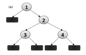
Bottom-up induction of decision trees was first mentioned in [59]. The authors propose a strategy that resembles agglomerative hierarchical clustering. The algorithm starts with each leaf having objects of the same class. In that way, a $k$-class

problem will generate a decision tree with $k$ leaves. The key idea is to merge, recursively, the two most similar classes in a non-terminal node. Then, a hyperplane is associated to the new non-terminal node, much in the same way as in top-down induction of oblique trees (in [59], a linear discriminant analysis procedure generates the hyperplanes). Next, all objects in the new non-terminal node are considered to be members of the same class (an artificial class that embodies the two clustered classes), and the procedure evaluates once again which are the two most similar classes. By recursively repeating this strategy, we end up with a decision tree in which the more obvious discriminations are done first, and the more subtle distinctions are postponed to lower levels. Landeweerd et al. [59] propose using the Mahalanobis distance to evaluate similarity among classes:
where $\mu_{y_{i}}$ is the mean attribute vector of class $y_{i}$ and $\Sigma$ is the covariance matrix pooled over all classes.

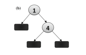
Some obvious drawbacks of this strategy of bottom-up induction are: (i) binaryclass problems provide a l-level decision tree (root node and two children); such a simple tree cannot model complex problems; (ii) instances from the same class may be located in very distinct regions of the attribute space, harming the initial assumption that instances from the same class should be located in the same leaf node; (iii) hierarchical clustering and hyperplane generation are costly operations; in fact, a procedure for inverting the covariance matrix in the Mahalanobis distance is usually of time complexity proportional to $O\left(n^{3}\right) .^{5}$ We believe these issues are among the main reasons why bottom-up induction has not become as popular as topdown induction. For alleviating these problems, Barros et al. [4] propose a bottom-up induction algorithm named BUTIA that combines EM clustering with SVM classifiers. The authors later generalize BUTIA to a framework for generating oblique decision trees, namely BUTIF [5], which allows the application of different clustering and classification strategies.

Hybrid induction was investigated in [56]. The ideia is to combine both bottom-up and top-down approaches for building the final decision tree. The algorithm starts by executing the bottom-up approach as described above until two subgroups are achieved. Then, two centers (mean attribute vectors) and covariance information are extracted from these subgroups and used for dividing the training data in a topdown fashion according to a normalized sum-of-squared-error criterion. If the two new partitions induced account for separated classes, then the hybrid induction is finished; otherwise, for each subgroup that does not account for a class, recursively executes the hybrid induction by once again starting with the bottom-up procedure. Kim and Landgrebe [56] argue that in hybrid induction “It is more likely to converge to classes of informational value, because the clustering initialization provides early

guidance in that direction, while the straightforward top-down approach does not guarantee such convergence”.

Several studies attempted on avoiding the greedy strategy usually employed for inducing trees. For instance, lookahead was employed for trying to improve greedy induction $[17,23,29,79,84]$. Murthy and Salzberg [79] show that one-level lookahead does not help building significantly better trees and can actually worsen the quality of trees induced. A more recent strategy for avoiding greedy decision-tree induction is to generate decision trees through evolutionary algorithms. The idea involved is to consider each decision tree as an individual in a population, which is evolved through a certain number of generations. Decision trees are modified by genetic operators, which are performed stochastically. A thorough review of decisiontree induction through evolutionary algorithms is presented in [6].

机器学习代写|决策树作业代写decision tree代考|Chapter Remarks

In this chapter, we presented the main design choices one has to face when programming a decision-tree induction algorithm. We gave special emphasis to the greedy top-down induction strategy, since it is by far the most researched technique for decision-tree induction.

Regarding top-down induction, we presented the most well-known splitting measures for univariate decision trees, as well as some new criteria found in the literature, in an unified notation. Furthermore, we introduced some strategies for building decision trees with multivariate tests, the so-called oblique trees. In particular, we showed that efficient oblique decision-tree induction has to make use of heuristics in order to derive “good” hyperplanes within non-terminal nodes. We detailed the strategy employed in the $\mathrm{OCl}$ algorithm $[77,80]$ for deriving hyperplanes with the help of a randomized perturbation process. Following, we depicted the most common stopping criteria and post-pruning techniques employed in classic algorithms such as CART [12] and C4.5 [89], and we ended the discussion on top-down induction with an enumeration of possible strategies for dealing with missing values, either in the growing phase or during classification of a new instance.

We ended our analysis on decision trees with some alternative induction strategies, such as bottom-up induction and hybrid-induction. In addition, we briefly discussed work that attempt to avoid the greedy strategy, by either implementing lookahead techniques, evolutionary algorithms, beam-search, linear programming, (non-) incremental restructuring, skewing, or anytime learning. In the next chapters, we present an overview of evolutionary algorithms and hyper-heuristics, and review how they can be applied to decision-tree induction.

机器学习代写|决策树作业代写decision tree代考|Evolutionary Algorithms

Evolutionary algorithms (EAs) are a collection of optimisation techniques whose design is based on metaphors of biological processes. Fretias [20] defines EAs as “stochastic search algorithms inspired by the process of neo-Darwinian evolution”, and Weise [44] states that “EAs are population-based metaheuristic optimisation algorithms that use biology-inspired mechanisms (…) in order to refine a set of solution candidates iteratively”.

The idea surrounding EAs is the following. There is a population of individuals, where each individual is a possible solution to a given problem. This population evolves towards increasingly better solutions through stochastic operators. After the evolution is completed, the fittest individual represents a “near-optimal” solution for the problem at hand.

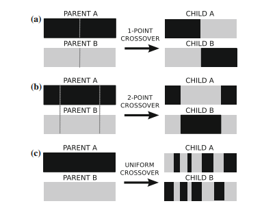
For evolving individuals, an EA evaluates each individual through a fitness function that measures the quality of the solutions that are being evolved. After the evaluation of all individuals that are part of the initial population, the algorithm’s iterative process starts. At each iteration, hereby called generation, the fittest individuals have a higher probability of being selected for reproduction to increase the chances of producing good solutions. The selected individuals undergo stochastic genetic operators, such as crossover and mutation, producing new offspring. These new individuals will replace the current population of individuals and the evolutionary process continues until a stopping criterion is satisfied (e.g., until a fixed number of generations is achieved, or until a satisfactory solution has been found).

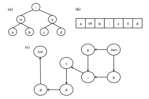
There are several kinds of EAs, such as genetic algorithms (GAs), genetic programming (GP), classifier systems (CS), evolution strategies (ES), evolutionary programming (EP), estimation of distribution algorithms (EDA), etc. This chapter will focus on GA and GP, the most commonly used EAs for data mining [19]. At a high level of abstraction, GAs and GP can be described by the pseudocode in Algorithm $1 .$

机器学习代写|决策树作业代写decision tree代考|Other Induction Strategies

决策树代写

机器学习代写|决策树作业代写decision tree代考|Other Induction Strategies

我们在上一节中对用于归纳决策树的贪心自上而下策略进行了全面回顾。在本节中,我们简要介绍了诱导决策树的替代策略。

决策树的自下而上归纳在 [59] 中首次提到。作者提出了一种类似于凝聚层次聚类的策略。该算法从每个叶子具有相同类的对象开始。这样,一个ķ-班级

问题将生成一个决策树ķ树叶。关键思想是递归地合并非终端节点中两个最相似的类。然后,超平面与新的非终端节点相关联,这与自上而下的倾斜树归纳方法非常相似(在 [59] 中,线性判别分析程序生成超平面)。接下来,新的非终端节点中的所有对象都被认为是同一类的成员(体现两个聚类类的人工类),并且该过程再次评估哪些是两个最相似的类。通过递归重复这个策略,我们最终得到一个决策树,其中首先进行更明显的区分,而将更细微的区分推迟到较低级别。兰德维尔德等人。[59] 建议使用马氏距离来评估类之间的相似性:
在哪里μ是一世是类的平均属性向量是一世和Σ是汇集在所有类上的协方差矩阵。

这种自下而上归纳策略的一些明显缺点是:(i)二元类问题提供了一个 l 级决策树(根节点和两个孩子);这样一棵简单的树不能模拟复杂的问题;(ii) 来自同一类的实例可能位于属性空间的非常不同的区域,损害了来自同一类的实例应该位于同一叶节点的初始假设;(iii) 层次聚类和超平面生成是昂贵的操作;事实上,在马氏距离中反转协方差矩阵的过程通常与时间复杂度成正比这(n3).5我们认为这些问题是自下而上归纳没有像自上而下归纳那样流行的主要原因之一。为了缓解这些问题,Barros 等人。[4] 提出了一种名为 BUTIA 的自下而上的归纳算法,它将 EM 聚类与 SVM 分类器相结合。作者后来将 BUTIA 推广到生成倾斜决策树的框架,即 BUTIF [5],它允许应用不同的聚类和分类策略。

在[56]中研究了混合诱导。想法是结合自下而上和自上而下的方法来构建最终的决策树。该算法首先执行如上所述的自下而上方法,直到获得两个子组。然后,从这些子组中提取两个中心(平均属性向量)和协方差信息,并用于根据归一化误差平方和标准以自上而下的方式划分训练数据。如果这两个新的分区导致了分离的类,那么混合归纳就结束了;否则,对于每个不考虑类的子组,通过再次从自下而上过程开始递归地执行混合归纳。Kim 和 Landgrebe [56] 认为,在混合归纳中,“它更有可能收敛到信息价值类别,

在这个方向上提供指导,而直接的自上而下的方法并不能保证这种趋同”。

一些研究试图避免通常用于诱导树的贪婪策略。例如,前瞻被用于试图改进贪婪归纳[17,23,29,79,84]. Murthy 和 Salzberg [79] 表明,一级前瞻无助于构建明显更好的树木,实际上会恶化诱导的树木质量。最近避免贪婪决策树归纳的策略是通过进化算法生成决策树。所涉及的想法是将每个决策树视为群体中的一个个体,它是通过一定数量的世代进化而来的。决策树由随机执行的遗传算子修改。[6] 中介绍了通过进化算法对决策树归纳的全面回顾。

机器学习代写|决策树作业代写decision tree代考|Chapter Remarks

在本章中,我们介绍了在编写决策树归纳算法时必须面对的主要设计选择。我们特别强调了贪心自上而下的归纳策略,因为它是迄今为止研究最多的决策树归纳技术。

关于自上而下的归纳,我们提出了最知名的单变量决策树拆分度量,以及文献中发现的一些新标准,以统一的符号表示。此外,我们介绍了一些用于构建具有多变量测试的决策树的策略,即所谓的倾斜树。特别是,我们展示了有效的倾斜决策树归纳必须利用启发式算法才能在非终端节点内推导出“好的”超平面。我们详细介绍了这Cl算法[77,80]用于在随机扰动过程的帮助下推导超平面。接下来,我们描述了 CART [12] 和 C4.5 [89] 等经典算法中使用的最常见的停止标准和后剪枝技术,并通过列举可能的处理策略来结束关于自上而下归纳的讨论缺少值,无论是在成长阶段还是在新实例的分类过程中。

我们用一些替代的归纳策略结束了对决策树的分析,例如自下而上的归纳和混合归纳。此外,我们简要讨论了试图通过实施前瞻技术、进化算法、波束搜索、线性规划、(非)增量重组、倾斜或随时学习来避免贪婪策略的工作。在接下来的章节中,我们将概述进化算法和超启发式,并回顾如何将它们应用于决策树归纳。

机器学习代写|决策树作业代写decision tree代考|Evolutionary Algorithms

进化算法 (EA) 是一组优化技术,其设计基于生物过程的隐喻。Fretias [20] 将 EA 定义为“受新达尔文进化过程启发的随机搜索算法”,Weise [44] 指出,“EA 是基于群体的元启发式优化算法,它使用受生物学启发的机制 (…)迭代地细化一组候选解决方案”。

围绕 EA 的想法如下。有一群人,其中每个人都是给定问题的可能解决方案。这个群体通过随机算子向越来越好的解决方案发展。进化完成后,最适合的个体代表手头问题的“接近最佳”解决方案。

对于进化中的个体,EA 通过一个适应度函数来评估每个个体,该函数测量正在进化的解决方案的质量。在对属于初始种群的所有个体进行评估后,算法的迭代过程开始。在每次迭代中,在此称为生成,最适合的个体有更高的概率被选中进行繁殖,以增加产生良好解决方案的机会。选定的个体经过随机遗传算子,例如交叉和突变,产生新的后代。这些新个体将取代当前个体种群并且进化过程继续直到满足停止标准(例如,直到达到固定数量的世代,或直到找到令人满意的解决方案)。

EA有几种类型,如遗传算法(GAs)、遗传编程(GP)、分类系统(CS)、进化策略(ES)、进化编程(EP)、分布估计算法(EDA)等。本章将重点介绍 GA 和 GP,这是数据挖掘中最常用的 EA [19]。在高抽象层次上,GAs 和 GP 可以用 Algorithm 中的伪代码来描述1.

机器学习代写|决策树作业代写decision tree代考 请认准statistics-lab™

统计代写请认准statistics-lab™. statistics-lab™为您的留学生涯保驾护航。

金融工程代写

金融工程是使用数学技术来解决金融问题。金融工程使用计算机科学、统计学、经济学和应用数学领域的工具和知识来解决当前的金融问题,以及设计新的和创新的金融产品。

非参数统计代写

非参数统计指的是一种统计方法,其中不假设数据来自于由少数参数决定的规定模型;这种模型的例子包括正态分布模型和线性回归模型。

广义线性模型代考

广义线性模型(GLM)归属统计学领域,是一种应用灵活的线性回归模型。该模型允许因变量的偏差分布有除了正态分布之外的其它分布。

术语 广义线性模型(GLM)通常是指给定连续和/或分类预测因素的连续响应变量的常规线性回归模型。它包括多元线性回归,以及方差分析和方差分析(仅含固定效应)。

有限元方法代写

有限元方法(FEM)是一种流行的方法,用于数值解决工程和数学建模中出现的微分方程。典型的问题领域包括结构分析、传热、流体流动、质量运输和电磁势等传统领域。

有限元是一种通用的数值方法,用于解决两个或三个空间变量的偏微分方程(即一些边界值问题)。为了解决一个问题,有限元将一个大系统细分为更小、更简单的部分,称为有限元。这是通过在空间维度上的特定空间离散化来实现的,它是通过构建对象的网格来实现的:用于求解的数值域,它有有限数量的点。边界值问题的有限元方法表述最终导致一个代数方程组。该方法在域上对未知函数进行逼近。[1] 然后将模拟这些有限元的简单方程组合成一个更大的方程系统,以模拟整个问题。然后,有限元通过变化微积分使相关的误差函数最小化来逼近一个解决方案。

tatistics-lab作为专业的留学生服务机构,多年来已为美国、英国、加拿大、澳洲等留学热门地的学生提供专业的学术服务,包括但不限于Essay代写,Assignment代写,Dissertation代写,Report代写,小组作业代写,Proposal代写,Paper代写,Presentation代写,计算机作业代写,论文修改和润色,网课代做,exam代考等等。写作范围涵盖高中,本科,研究生等海外留学全阶段,辐射金融,经济学,会计学,审计学,管理学等全球99%专业科目。写作团队既有专业英语母语作者,也有海外名校硕博留学生,每位写作老师都拥有过硬的语言能力,专业的学科背景和学术写作经验。我们承诺100%原创,100%专业,100%准时,100%满意。

随机分析代写


随机微积分是数学的一个分支,对随机过程进行操作。它允许为随机过程的积分定义一个关于随机过程的一致的积分理论。这个领域是由日本数学家伊藤清在第二次世界大战期间创建并开始的。

时间序列分析代写

随机过程,是依赖于参数的一组随机变量的全体,参数通常是时间。 随机变量是随机现象的数量表现,其时间序列是一组按照时间发生先后顺序进行排列的数据点序列。通常一组时间序列的时间间隔为一恒定值(如1秒,5分钟,12小时,7天,1年),因此时间序列可以作为离散时间数据进行分析处理。研究时间序列数据的意义在于现实中,往往需要研究某个事物其随时间发展变化的规律。这就需要通过研究该事物过去发展的历史记录,以得到其自身发展的规律。

回归分析代写

多元回归分析渐进(Multiple Regression Analysis Asymptotics)属于计量经济学领域,主要是一种数学上的统计分析方法,可以分析复杂情况下各影响因素的数学关系,在自然科学、社会和经济学等多个领域内应用广泛。

MATLAB代写

MATLAB 是一种用于技术计算的高性能语言。它将计算、可视化和编程集成在一个易于使用的环境中,其中问题和解决方案以熟悉的数学符号表示。典型用途包括:数学和计算算法开发建模、仿真和原型制作数据分析、探索和可视化科学和工程图形应用程序开发,包括图形用户界面构建MATLAB 是一个交互式系统,其基本数据元素是一个不需要维度的数组。这使您可以解决许多技术计算问题,尤其是那些具有矩阵和向量公式的问题,而只需用 C 或 Fortran 等标量非交互式语言编写程序所需的时间的一小部分。MATLAB 名称代表矩阵实验室。MATLAB 最初的编写目的是提供对由 LINPACK 和 EISPACK 项目开发的矩阵软件的轻松访问,这两个项目共同代表了矩阵计算软件的最新技术。MATLAB 经过多年的发展,得到了许多用户的投入。在大学环境中,它是数学、工程和科学入门和高级课程的标准教学工具。在工业领域,MATLAB 是高效研究、开发和分析的首选工具。MATLAB 具有一系列称为工具箱的特定于应用程序的解决方案。对于大多数 MATLAB 用户来说非常重要,工具箱允许您学习应用专业技术。工具箱是 MATLAB 函数(M 文件)的综合集合,可扩展 MATLAB 环境以解决特定类别的问题。可用工具箱的领域包括信号处理、控制系统、神经网络、模糊逻辑、小波、仿真等。

R语言代写问卷设计与分析代写
PYTHON代写回归分析与线性模型代写
MATLAB代写方差分析与试验设计代写
STATA代写机器学习/统计学习代写
SPSS代写计量经济学代写
EVIEWS代写时间序列分析代写
EXCEL代写深度学习代写
SQL代写各种数据建模与可视化代写

机器学习代写|决策树作业代写decision tree代考|Cost-Complexity Pruning

如果你也在 怎样代写决策树decision tree这个学科遇到相关的难题,请随时右上角联系我们的24/7代写客服。

决策树是一种决策支持工具,它使用决策及其可能后果的树状模型,包括偶然事件结果、资源成本和效用。它是显示一个只包含条件控制语句的算法的一种方式。

statistics-lab™ 为您的留学生涯保驾护航 在代写决策树decision tree方面已经树立了自己的口碑, 保证靠谱, 高质且原创的统计Statistics代写服务。我们的专家在代写决策树decision tree代写方面经验极为丰富,各种代写决策树decision tree相关的作业也就用不着说。

我们提供的决策树decision tree及其相关学科的代写,服务范围广, 其中包括但不限于:

  • Statistical Inference 统计推断
  • Statistical Computing 统计计算
  • Advanced Probability Theory 高等概率论
  • Advanced Mathematical Statistics 高等数理统计学
  • (Generalized) Linear Models 广义线性模型
  • Statistical Machine Learning 统计机器学习
  • Longitudinal Data Analysis 纵向数据分析
  • Foundations of Data Science 数据科学基础
机器学习代写|决策树作业代写decision tree代考|Cost-Complexity Pruning

机器学习代写|决策树作业代写decision tree代考|Cost-Complexity Pruning

Cost-complexity pruning is the post-pruning strategy of the CART system, detailed in [12]. It consists of two steps:

  1. Generate a sequence of increasingly smaller trees, beginning with $T$ and ending with the root node of $T$, by successively pruning the subtree yielding the lowest cost complexity, in a bottom-up fashion;
  2. Choose the best tree among the sequence based on its relative size and accuracy (either on a pruning set, or provided by a cross-validation procedure in the training set).

The idea within step 1 is that pruned tree $T_{i+1}$ is obtained by pruning the subtrees that show the lowest increase in the apparent error (error in the training set) per pruned leaf. Since the apparent error of pruned node $t$ increases by the amount $r^{(t)}-r^{T^{(r)}}$, whereas its number of leaves decreases by $\left|\lambda_{T^{(t)}}\right|-1$ units, the following ratio measures the increase in apparent error rate per pruned leaf:
$$
\alpha=\frac{r^{(r)}-r^{T^{(t)}}}{\left|\lambda_{T^{(t)}}\right|-1}
$$
Therefore, $T_{i+1}$ is obtained by pruning all nodes in $T_{i}$ with the lowest value of $\alpha$. $T_{0}$ is obtained by pruning all nodes in $T$ whose $\alpha$ value is 0 . It is possible to show that each tree $T_{i}$ is associated to a distinct value $\alpha_{i}$, such that $\alpha_{i}<\alpha_{i+1}$. Building the sequence of trees in step 1 takes quadratic time with respect to the number of internal nodes.

Regarding step 2, CCP chooses the smallest tree whose error (either on the pruning set or on cross-validation) is not more than one standard error (SE) greater than the lowest error observed in the sequence of trees. This strategy is known as “1-SE” variant since the work of Esposito et al. [33], which proposes ignoring the standard error constraint, calling the strategy of selecting trees based only on accuracy of “0-SE”. It is argued that 1-SE has a tendency of overpruning trees, since its selection is based on a conservative constraint $[32,33]$.

机器学习代写|决策树作业代写decision tree代考|Error-Based Pruning

This strategy was proposed by Quinlan and it is implemented as the default pruning strategy of C4.5 [89]. It is an improvement over PEP, based on a far more pessimistic estimate of the expected error. Unlike PEP, EBP performs a bottom-up search, and it performs not only the replacement of non-terminal nodes by leaves but also the grafting $g^{4}$ of subtree $T^{(t)}$ onto the place of parent $t$. Grafting is exemplified in Fig. $2.2$.
Since grafting is potentially a time-consuming task, only the child subtree $T^{\left(t^{\prime}\right)}$ of $t$ with the greatest number of instances is considered to be grafted onto the place of $t$.

For deciding whether to replace a non-terminal node by a leaf (subtree replacement), to graft a subtree onto the place of its parent (subtree raising) or not to prune at all, a pessimistic estimate of the expected error is calculated by using an upper confidence bound. Assuming that errors in the training set are binomially distributed with a given probability $p$ in $N_{x}^{(t)}$ trials, it is possible to compute the exact value of the upper confidence bound as the value of $p$ for which a binomially distributed random variable $P$ shows $E^{(t)}$ successes in $N_{x}^{(t)}$ trials with probability $C F$. In other words, given a particular confidence $C F$ (C4.5 default value is $C F=25 \%$ ), we can find the upper bound of the expected error $\left(E E_{U B}\right)$ as follows:
$$
E E_{U B}=\frac{f+\frac{z^{2}}{2 N_{x}}+z \sqrt{\frac{f}{N_{x}}-\frac{f^{2}}{N_{x}}+\frac{z^{2}}{4 N_{x}^{2}}}}{1+\frac{z^{2}}{N_{x}}}
$$
where $f=E^{(t)} / N_{x}$ and $z$ is the number of standard deviations corresponding to the confidence $C F$ (e.g., for $C F=25 \%, z=0.69$ ).

In order to calculate the expected error of node $t\left(E E^{(t)}\right)$, one must simply compute $N_{x}^{(t)} \times E E_{U B}$. For evaluating a subtree $T^{(t)}$, one must sum the expected error of every leaf of that subtree, i.e., $\sum_{s \in \lambda_{T}(t)} E E^{(s)}$. Hence, given a non-terminal node $t$, it is possible to decide whether one should perform subtree replacement (when condition $E E^{(t)} \leq E E^{T^{(t)}}$ holds), subtree raising (when conditions $\exists j \in \zeta_{t}, E E^{(j)}<E E^{(t)} \wedge$ $\forall i \in \zeta_{I}, N_{x}^{(i)}<N_{x}^{(j)}$ hold), or not to prune $t$ otherwise.

An advantage of EBP is the new grafting operation that allows pruning useless branches without ignoring interesting lower branches (an elegant solution to the horizon effect problem). A drawback of the method is the parameter $C F$, even though it represents a confidence level. Smaller values of $C F$ result in more pruning.

机器学习代写|决策树作业代写decision tree代考|Empirical Evaluations

Some studies in the literature performed empirical analyses for evaluating pruning strategies. For instance, Quinlan [94] compared four methods of tree pruning (three of them presented in the previous sections-REP, PEP and CCP 1-SE). He argued that those methods in which a pruning set is needed (REP and CCP) did not perform noticeably better than the other methods, and thus their requirement for additional data is a weakness.

Mingers [71] compared five pruning methods, all of them presented in the previous sections (CCP, CVP, MEP, REP and PEP), and related them to different splitting measures. He states that pruning can improve the accuracy of induced decision trees by up to $25 \%$ in domains with noise and residual variation. In addition, he highlights the following findings: (i) MEP (the original version by Niblett and Bratko [82]) is the least accurate method due to its sensitivity to the number of classes in the data; (ii) PEP is the most “crude” strategy, though the fastest one-due to some bad results,

it should be used with caution; (iii) CVP, CCP and REP performed well, providing consistently low error-rates for all data sets used; and (iv) there is no evidence of an interaction between the splitting measure and the pruning method used for inducing a decision tree.

Buntine [16], in his PhD thesis, also reports experiments on pruning methods (PEP, MEP, CCP 0-SE and 1-SE for both pruning set and cross-validation). Some of his findings were: (i) CCP $0-S E$ versions were marginally superior than the $1-S E$ versions; (ii) CCP 1-SE versions were superior in data sets with little apparent structure, where more severe pruning was inherently better; (iii) CCP 0-SE with crossvalidation was marginally better than the other methods, though not in all data sets; and (iv) PEP performed reasonably well in all data sets, and was significantly superior in well-structured data sets (mushroom, glass and LED, all from UCI [36]);

Esposito et al. [32] compare the six post-pruning methods presented in the previous sections within an extended C4.5 system. Their findings were the following: (i) MEP, CVP, and EBP tend to underprune, whereas 1-SE (both cross-validation and pruning set versions) and REP have a propensity for overpruning; (ii) using a pruning-set is not usually a good option; (iii) PEP and EBP behave similarly, despite the difference in their formulation; (iv) pruning does not generally decrease the accuracy of a decision tree (only one of the domains tested was deemed as “pruning-averse”); and (v) data sets not prone to pruning are usually the ones with the highest base error whereas data sets with a low base error tend to benefit of any pruning strategy.

For a comprehensive survey of strategies for simplifying decision trees, please refer to [13]. For more details on post-pruning techniques in decision trees for regression, we recommend $[12,54,85,97,113-115]$.

机器学习代写|决策树作业代写decision tree代考|Cost-Complexity Pruning

决策树代写

机器学习代写|决策树作业代写decision tree代考|Cost-Complexity Pruning

成本复杂度剪枝是 CART 系统的后剪枝策略,详见 [12]。它由两个步骤组成:

  1. 生成一系列越来越小的树,从吨并以根节点结束吨,通过以自下而上的方式连续修剪产生最低成本复杂度的子树;
  2. 根据其相对大小和准确性(在修剪集上,或由训练集中的交叉验证程序提供)在序列中选择最佳树。

第 1 步中的想法是修剪过的树吨一世+1通过修剪显示每个修剪叶的明显误差(训练集中的误差)增加最低的子树来获得。由于修剪节点的明显错误吨增加金额r(吨)−r吨(r),而它的叶子数量减少了|λ吨(吨)|−1单位,以下比率衡量每个修剪过的叶子的明显错误率的增加:
一种=r(r)−r吨(吨)|λ吨(吨)|−1
所以,吨一世+1通过修剪所有节点获得吨一世具有最低值一种. 吨0通过修剪所有节点获得吨谁的一种值为 0 。可以证明每棵树吨一世与不同的值相关联一种一世, 这样一种一世<一种一世+1. 在步骤 1 中构建树序列需要与内部节点数量成二次方的时间。

关于步骤 2,CCP 选择最小的树,其误差(在修剪集或交叉验证上)不超过一个标准误差 (SE),大于在树序列中观察到的最低误差。由于 Esposito 等人的工作,这种策略被称为“1-SE”变体。[33],它提出忽略标准误差约束,调用仅基于“0-SE”精度的选择树的策略。有人认为 1-SE 具有过度修剪树的趋势,因为它的选择是基于保守约束[32,33].

机器学习代写|决策树作业代写decision tree代考|Error-Based Pruning

该策略由 Quinlan 提出,并作为 C4.5 [89] 的默认剪枝策略实现。它是对 PEP 的改进,基于对预期误差的更为悲观的估计。与 PEP 不同,EBP 执行自下而上的搜索,它不仅执行非终端节点的叶子替换,还执行嫁接G4子树的吨(吨)到父母的地方吨. 嫁接示例如图 1 所示。2.2.
由于嫁接可能是一项耗时的任务,因此只有子子树吨(吨′)的吨实例数最多的被认为是嫁接到吨.

为了决定是否用叶子替换非终端节点(子树替换),将子树嫁接到其父节点的位置(子树提升)或根本不修剪,通过使用计算预期误差的悲观估计置信上限。假设训练集中的错误以给定的概率呈二项式分布p在ñX(吨)试验,可以将置信上限的确切值计算为p一个二项分布的随机变量磷节目和(吨)成功ñX(吨)概率试验CF. 换句话说,给定一个特定的信心CF(C4.5 默认值为CF=25%),我们可以找到预期误差的上限(和和在乙)如下:
和和在乙=F+和22ñX+和FñX−F2ñX+和24ñX21+和2ñX
在哪里F=和(吨)/ñX和和是对应于置信度的标准差数CF(例如,对于CF=25%,和=0.69 ).

为了计算节点的预期误差吨(和和(吨)), 必须简单地计算ñX(吨)×和和在乙. 用于评估子树吨(吨),必须将该子树的每个叶子的预期误差求和,即∑s∈λ吨(吨)和和(s). 因此,给定一个非终端节点吨,可以决定是否应该执行子树替换(当条件和和(吨)≤和和吨(吨)成立),子树提升(当条件∃j∈G吨,和和(j)<和和(吨)∧ ∀一世∈G一世,ñX(一世)<ñX(j)持有),或不修剪吨除此以外。

EBP 的一个优点是新的嫁接操作,它允许修剪无用的分支而不会忽略有趣的较低分支(对地平线效应问题的优雅解决方案)。该方法的一个缺点是参数CF,即使它代表一个置信水平。较小的值CF导致更多的修剪。

机器学习代写|决策树作业代写decision tree代考|Empirical Evaluations

文献中的一些研究对评估修剪策略进行了实证分析。例如,Quinlan [94] 比较了四种树修剪方法(其中三种在前面的章节中介绍过——REP、PEP 和 CCP 1-SE)。他认为,那些需要修剪集的方法(REP 和 CCP)的性能并没有明显优于其他方法,因此它们对额外数据的要求是一个弱点。

Mingers [71] 比较了五种修剪方法,所有这些方法都在前面的章节中介绍过(CCP、CVP、MEP、REP 和 PEP),并将它们与不同的分裂措施相关联。他指出,剪枝可以将诱导决策树的准确性提高多达25%在具有噪声和残余变化的域中。此外,他强调了以下发现:(i)MEP(Niblett 和 Bratko [82] 的原始版本)是最不准确的方法,因为它对数据中的类数很敏感;(ii) PEP 是最“粗鲁”的策略,虽然是最快的策略——由于一些糟糕的结果,

应谨慎使用;(iii) CVP、CCP 和 REP 表现良好,为所有使用的数据集提供始终如一的低错误率;(iv) 没有证据表明分裂度量和用于诱导决策树的修剪方法之间存在相互作用。

Buntine [16] 在他的博士论文中还报告了剪枝方法的实验(PEP、MEP、CCP 0-SE 和 1-SE 用于剪枝集和交叉验证)。他的一些发现是:(i) CCP0−小号和版本略优于1−小号和版本;(ii) CCP 1-SE 版本在几乎没有明显结构的数据集中表现出色,其中更严格的修剪本质上更好;(iii) 具有交叉验证的 CCP 0-SE 略好于其他方法,尽管并非在所有数据集中;(iv) PEP 在所有数据集中表现相当不错,并且在结构良好的数据集中(蘑菇、玻璃和 LED,均来自 UCI [36])显着优于;

埃斯波西托等人。[32] 在扩展的 C4.5 系统中比较了前几节中介绍的六种后修剪方法。他们的发现如下:(i)MEP、CVP 和 EBP 倾向于欠修剪,而 1-SE(交叉验证和修剪集版本)和 REP 有过度修剪的倾向;(ii) 使用剪枝集通常不是一个好的选择;(iii) PEP 和 EBP 的行为相似,尽管它们的表述不同;(iv) 修剪通常不会降低决策树的准确性(只有一个测试域被认为是“厌恶修剪”);(v) 不易修剪的数据集通常是具有最高基误差的数据集,而具有低基误差的数据集往往会受益于任何修剪策略。

有关简化决策树的策略的全面调查,请参阅[13]。有关回归决策树中的后修剪技术的更多详细信息,我们建议[12,54,85,97,113−115].

机器学习代写|决策树作业代写decision tree代考 请认准statistics-lab™

统计代写请认准statistics-lab™. statistics-lab™为您的留学生涯保驾护航。

金融工程代写

金融工程是使用数学技术来解决金融问题。金融工程使用计算机科学、统计学、经济学和应用数学领域的工具和知识来解决当前的金融问题,以及设计新的和创新的金融产品。

非参数统计代写

非参数统计指的是一种统计方法,其中不假设数据来自于由少数参数决定的规定模型;这种模型的例子包括正态分布模型和线性回归模型。

广义线性模型代考

广义线性模型(GLM)归属统计学领域,是一种应用灵活的线性回归模型。该模型允许因变量的偏差分布有除了正态分布之外的其它分布。

术语 广义线性模型(GLM)通常是指给定连续和/或分类预测因素的连续响应变量的常规线性回归模型。它包括多元线性回归,以及方差分析和方差分析(仅含固定效应)。

有限元方法代写

有限元方法(FEM)是一种流行的方法,用于数值解决工程和数学建模中出现的微分方程。典型的问题领域包括结构分析、传热、流体流动、质量运输和电磁势等传统领域。

有限元是一种通用的数值方法,用于解决两个或三个空间变量的偏微分方程(即一些边界值问题)。为了解决一个问题,有限元将一个大系统细分为更小、更简单的部分,称为有限元。这是通过在空间维度上的特定空间离散化来实现的,它是通过构建对象的网格来实现的:用于求解的数值域,它有有限数量的点。边界值问题的有限元方法表述最终导致一个代数方程组。该方法在域上对未知函数进行逼近。[1] 然后将模拟这些有限元的简单方程组合成一个更大的方程系统,以模拟整个问题。然后,有限元通过变化微积分使相关的误差函数最小化来逼近一个解决方案。

tatistics-lab作为专业的留学生服务机构,多年来已为美国、英国、加拿大、澳洲等留学热门地的学生提供专业的学术服务,包括但不限于Essay代写,Assignment代写,Dissertation代写,Report代写,小组作业代写,Proposal代写,Paper代写,Presentation代写,计算机作业代写,论文修改和润色,网课代做,exam代考等等。写作范围涵盖高中,本科,研究生等海外留学全阶段,辐射金融,经济学,会计学,审计学,管理学等全球99%专业科目。写作团队既有专业英语母语作者,也有海外名校硕博留学生,每位写作老师都拥有过硬的语言能力,专业的学科背景和学术写作经验。我们承诺100%原创,100%专业,100%准时,100%满意。

随机分析代写


随机微积分是数学的一个分支,对随机过程进行操作。它允许为随机过程的积分定义一个关于随机过程的一致的积分理论。这个领域是由日本数学家伊藤清在第二次世界大战期间创建并开始的。

时间序列分析代写

随机过程,是依赖于参数的一组随机变量的全体,参数通常是时间。 随机变量是随机现象的数量表现,其时间序列是一组按照时间发生先后顺序进行排列的数据点序列。通常一组时间序列的时间间隔为一恒定值(如1秒,5分钟,12小时,7天,1年),因此时间序列可以作为离散时间数据进行分析处理。研究时间序列数据的意义在于现实中,往往需要研究某个事物其随时间发展变化的规律。这就需要通过研究该事物过去发展的历史记录,以得到其自身发展的规律。

回归分析代写

多元回归分析渐进(Multiple Regression Analysis Asymptotics)属于计量经济学领域,主要是一种数学上的统计分析方法,可以分析复杂情况下各影响因素的数学关系,在自然科学、社会和经济学等多个领域内应用广泛。

MATLAB代写

MATLAB 是一种用于技术计算的高性能语言。它将计算、可视化和编程集成在一个易于使用的环境中,其中问题和解决方案以熟悉的数学符号表示。典型用途包括:数学和计算算法开发建模、仿真和原型制作数据分析、探索和可视化科学和工程图形应用程序开发,包括图形用户界面构建MATLAB 是一个交互式系统,其基本数据元素是一个不需要维度的数组。这使您可以解决许多技术计算问题,尤其是那些具有矩阵和向量公式的问题,而只需用 C 或 Fortran 等标量非交互式语言编写程序所需的时间的一小部分。MATLAB 名称代表矩阵实验室。MATLAB 最初的编写目的是提供对由 LINPACK 和 EISPACK 项目开发的矩阵软件的轻松访问,这两个项目共同代表了矩阵计算软件的最新技术。MATLAB 经过多年的发展,得到了许多用户的投入。在大学环境中,它是数学、工程和科学入门和高级课程的标准教学工具。在工业领域,MATLAB 是高效研究、开发和分析的首选工具。MATLAB 具有一系列称为工具箱的特定于应用程序的解决方案。对于大多数 MATLAB 用户来说非常重要,工具箱允许您学习应用专业技术。工具箱是 MATLAB 函数(M 文件)的综合集合,可扩展 MATLAB 环境以解决特定类别的问题。可用工具箱的领域包括信号处理、控制系统、神经网络、模糊逻辑、小波、仿真等。

R语言代写问卷设计与分析代写
PYTHON代写回归分析与线性模型代写
MATLAB代写方差分析与试验设计代写
STATA代写机器学习/统计学习代写
SPSS代写计量经济学代写
EVIEWS代写时间序列分析代写
EXCEL代写深度学习代写
SQL代写各种数据建模与可视化代写

机器学习代写|决策树作业代写decision tree代考|Pruning

如果你也在 怎样代写决策树decision tree这个学科遇到相关的难题,请随时右上角联系我们的24/7代写客服。

决策树是一种决策支持工具,它使用决策及其可能后果的树状模型,包括偶然事件结果、资源成本和效用。它是显示一个只包含条件控制语句的算法的一种方式。

statistics-lab™ 为您的留学生涯保驾护航 在代写决策树decision tree方面已经树立了自己的口碑, 保证靠谱, 高质且原创的统计Statistics代写服务。我们的专家在代写决策树decision tree代写方面经验极为丰富,各种代写决策树decision tree相关的作业也就用不着说。

我们提供的决策树decision tree及其相关学科的代写,服务范围广, 其中包括但不限于:

  • Statistical Inference 统计推断
  • Statistical Computing 统计计算
  • Advanced Probability Theory 高等概率论
  • Advanced Mathematical Statistics 高等数理统计学
  • (Generalized) Linear Models 广义线性模型
  • Statistical Machine Learning 统计机器学习
  • Longitudinal Data Analysis 纵向数据分析
  • Foundations of Data Science 数据科学基础
Decision Trees - Mihail Eric
机器学习代写|决策树作业代写decision tree代考|Pruning

机器学习代写|决策树作业代写decision tree代考|Reduced-Error Pruning

Reduced-error pruning is a conceptually simple strategy proposed by Quinlan [94]. It uses a pruning set (a part of the training set) to evaluate the goodness of a given subtree from $T$. The idea is to evaluate each non-terminal node $t \in \zeta_{T}$ with regard to the classification error in the pruning set. If such an error decreases when we replace the subtree $T^{(t)}$ by a leaf node, than $T^{(t)}$ must be pruned.

Quinlan imposes a constraint: a node $t$ cannot be pruned if it contains a subtree that yields a lower classification error in the pruning set. The practical consequence of this constraint is that REP should be performed in a bottom-up fashion. The REP pruned tree $T^{\prime}$ presents an interesting optimality property: it is the smallest most accurate tree resulting from pruning original tree $T$ [94]. Besides this optimality property, another advantage of REP is its linear complexity, since each node is visited only once in $T$. An obvious disadvantage is the need of using a pruning set, which means one has to divide the original training set, resulting in less instances to grow the tree. This disadvantage is particularly serious for small data sets.

机器学习代写|决策树作业代写decision tree代考|Pessimistic Error Pruning

Also proposed by Quinlan [94], the pessimistic error pruning uses the training set for both growing and pruning the tree. The apparent error rate, i.e., the error rate calculated over the training set, is optimistically biased and cannot be used to decide whether pruning should be performed or not. Quinlan thus proposes adjusting the apparent error according to the continuity correction for the binomial distribution (cc) in order to provide a more realistic error rate. Consider the apparent error of a pruned node $t$, and the error of its entire subtree $T^{(t)}$ before pruning is performed, respectively:
$$
\begin{aligned}
r^{(t)} &=\frac{E^{(t)}}{N_{x}^{(t)}} \
r^{T^{(t)}} &=\frac{\sum_{s \in \lambda_{T^{(t)}}} E^{(s)}}{\sum_{s \in \lambda_{T^{(t)}}} N_{x}^{(s)}} .
\end{aligned}
$$
Modifying (2.33) and (2.34) according to $c c$ results in:
$$
\begin{gathered}
r_{c c}^{(t)}=\frac{E^{(t)}+1 / 2}{N_{x}^{(t)}} \
r_{c c}^{T^{(t)}}=\frac{\sum_{s \in \lambda_{T}(t)} E^{(s)}+1 / 2}{\sum_{s \in \lambda_{T}(t)} N_{x}^{(s)}}=\frac{\frac{\left|\lambda_{T(t)}\right|}{2} \sum_{s \in \lambda_{T(t)}} E^{(s)}}{\sum_{s \in \lambda_{T}(t)} N_{x}^{(s)}} .
\end{gathered}
$$
For the sake of simplicity, we will refer to the adjusted number of errors rather than the adjusted error rate, i.e., $E_{c c}^{(t)}=E^{(t)}+1 / 2$ and $E_{c c}^{T^{(t)}}=\left(\left|\lambda_{T^{(t)}}\right| / 2\right) \sum_{s \in \lambda_{T^{(t)}}} E^{(s)}$. Ideally, pruning should occur if $E_{c c}^{(t)} \leq E_{c c}^{T^{(t)}}$, but note that this condition seldom holds, since the decision tree is usually grown up to the homogeneity stopping criterion (criterion 1 in Sect. 2.3.2), and thus $E_{c c}^{T^{(t)}}=\left|\lambda_{T^{(t)}}\right| / 2$ whereas $E_{c c}^{(t)}$ will very probably be a higher value. In fact, due to the homogeneity stopping criterion, $E_{c c}^{T^{(t)}}$ becomes simply a measure of complexity which associates each leaf node with a cost of $1 / 2$. Quinlan, aware of this situation, weakens the original condition a

$$
E_{c c}^{(t)} \leq E_{c c}^{T^{(t)}}
$$
to
$$
E_{c c}^{(t)} \leq E_{c c}^{T^{(t)}}+S E\left(E_{c c}^{T^{(\mathrm{r})}}\right)
$$
where
$$
S E\left(E_{c c}^{T^{(t)}}\right)=\sqrt{\frac{E_{c c}^{T^{(t)}} *\left(N_{x}^{(t)}-E_{c c}^{T^{(t)}}\right)}{N_{x}^{(t)}}}
$$
is the standard error for the subtree $T^{(t)}$, computed as if the distribution of errors were binomial.

PEP is computed in a top-down fashion, and if a given node $t$ is pruned, its descendants are not examined, which makes this pruning strategy quite efficient in terms of computational effort. As a point of criticism, Esposito et al. [32] point out that the introduction of the continuity correction in the estimation of the error rate has no theoretical justification, since it was never applied to correct over-optimistic estimates of error rates in statistics.

机器学习代写|决策树作业代写decision tree代考|Minimum Error Pruning

Originally proposed by Niblett and Bratko [82] and further extended by Cestnik and Bartko [19], minimum error pruning is a bottom-up approach that seeks to minimize the expected error rate for unseen cases. It estimates the expected error rate in node $t\left(E E^{(t)}\right)$ as follows:
$$
E E^{(t)}=\min {\xi M}\left[\frac{N{x}^{(t)}-N_{\bullet, y y^{(t)}}^{(t)}+\left(1-p_{\bullet}^{(t)}\right) \times m}{N_{x}^{(t)}+m}\right] .
$$
where $m$ is a parameter that determines the importance of the a priori probability on the estimation of the error. Eq. (2.39), presented in [19], is a generalisation of the expected error rate presented in [82] if we assume that $m=k$ and that $p_{\bullet}^{(t)}=$ $1 / k, \forall y_{n} \in Y$.

MEP is performed by comparing $E E^{(t)}$ with the weighted sum of the expected error rate of all children nodes from $t$. Each weight is given by $p_{y_{j}, \boldsymbol{e}}$, assuming $v_{j}$ is the partition corresponding to the $j$ th child of $t$. A disadvantage of MEP is the need of setting the ad-hoc parameter $m$. Usually, the higher the value of $m$, the more severe the pruning. Cestnik and Bratko [19] suggest that a domain expert should set $m$ according to the level of noise in the data. Alternatively, a set of trees pruned with different values of $m$ could be offered to the domain expert, so he/she can choose the best one according to his/her experience.

SAS Help Center: Pruning
机器学习代写|决策树作业代写decision tree代考|Pruning

决策树代写

机器学习代写|决策树作业代写decision tree代考|Reduced-Error Pruning

减少错误修剪是 Quinlan [94] 提出的概念上简单的策略。它使用修剪集(训练集的一部分)来评估给定子树的优度吨. 这个想法是评估每个非终端节点吨∈G吨关于剪枝集中的分类误差。如果我们替换子树时这样的错误减少了吨(吨)通过一个叶节点,比吨(吨)必须修剪。

Quinlan 施加了一个约束:一个节点吨如果它包含在修剪集中产生较低分类错误的子树,则无法修剪。这种约束的实际结果是 REP 应该以自下而上的方式执行。REP 修剪树吨′提出了一个有趣的最优性:它是修剪原始树得到的最小最准确的树吨[94]。除了这个最优性之外,REP 的另一个优点是它的线性复杂性,因为每个节点只被访问一次吨. 一个明显的缺点是需要使用剪枝集,这意味着必须分割原始训练集,导致生成树的实例更少。这个缺点对于小数据集尤其严重。

机器学习代写|决策树作业代写decision tree代考|Pessimistic Error Pruning

Quinlan [94] 也提出,悲观错误修剪使用训练集来生长和修剪树。表观错误率,即在训练集上计算的错误率,具有乐观偏差,不能用于决定是否应该进行剪枝。因此,Quinlan 建议根据二项式分布 (cc) 的连续性校正来调整表观误差,以提供更真实的错误率。考虑修剪节点的明显错误吨, 及其整个子树的误差吨(吨)在进行剪枝之前,分别为:
r(吨)=和(吨)ñX(吨) r吨(吨)=∑s∈λ吨(吨)和(s)∑s∈λ吨(吨)ñX(s).
修改 (2.33) 和 (2.34) 根据CC结果是:
rCC(吨)=和(吨)+1/2ñX(吨) rCC吨(吨)=∑s∈λ吨(吨)和(s)+1/2∑s∈λ吨(吨)ñX(s)=|λ吨(吨)|2∑s∈λ吨(吨)和(s)∑s∈λ吨(吨)ñX(s).
为简单起见,我们将参考调整后的错误数而不是调整后的错误率,即和CC(吨)=和(吨)+1/2和和CC吨(吨)=(|λ吨(吨)|/2)∑s∈λ吨(吨)和(s). 理想情况下,修剪应该发生在和CC(吨)≤和CC吨(吨),但请注意,这种情况很少成立,因为决策树通常会长大到同质性停止标准(第 2.3.2 节中的标准 1),因此和CC吨(吨)=|λ吨(吨)|/2然而和CC(吨)很可能会是一个更高的价值。事实上,由于同质性停止准则,和CC吨(吨)成为简单的复杂性度量,它将每个叶节点与成本相关联1/2. 昆兰意识到这种情况,削弱了原有的条件和CC(吨)≤和CC吨(吨)

和CC(吨)≤和CC吨(吨)+小号和(和CC吨(r))
在哪里
小号和(和CC吨(吨))=和CC吨(吨)∗(ñX(吨)−和CC吨(吨))ñX(吨)
是子树的标准误差吨(吨), 计算得好像误差分布是二项式的。

PEP 以自上而下的方式计算,如果给定节点吨被修剪,它的后代没有被检查,这使得这种修剪策略在计算工作方面非常有效。作为一个批评点,Esposito 等人。[32] 指出,在错误率估计中引入连续性校正没有理论依据,因为它从未应用于纠正统计中错误率的过度乐观估计。

机器学习代写|决策树作业代写decision tree代考|Minimum Error Pruning

最初由 Niblett 和 Bratko [82] 提出,并由 Cestnik 和 Bartko [19] 进一步扩展,最小错误修剪是一种自下而上的方法,旨在最小化未见案例的预期错误率。它估计节点中的预期错误率吨(和和(吨))如下:
和和(吨)=分钟X米[ñX(吨)−ñ∙,是是(吨)(吨)+(1−p∙(吨))×米ñX(吨)+米].
在哪里米是一个参数,它决定了先验概率对误差估计的重要性。方程。[19] 中提出的 (2.39) 是 [82] 中提出的预期错误率的概括,如果我们假设米=ķ然后p∙(吨)= 1/ķ,∀是n∈是.

MEP 通过比较来执行和和(吨)与所有子节点的预期错误率的加权和吨. 每个权重由下式给出p是j,和, 假设在j是对应的分区j的第一个孩子吨. MEP 的一个缺点是需要设置 ad-hoc 参数米. 通常,值越高米,剪枝越严重。Cestnik 和 Bratko [19] 建议领域专家应该设置米根据数据中的噪声水平。或者,用不同的值修剪一组树米可以提供给领域专家,因此他/她可以根据自己的经验选择最好的。

机器学习代写|决策树作业代写decision tree代考 请认准statistics-lab™

统计代写请认准statistics-lab™. statistics-lab™为您的留学生涯保驾护航。

金融工程代写

金融工程是使用数学技术来解决金融问题。金融工程使用计算机科学、统计学、经济学和应用数学领域的工具和知识来解决当前的金融问题,以及设计新的和创新的金融产品。

非参数统计代写

非参数统计指的是一种统计方法,其中不假设数据来自于由少数参数决定的规定模型;这种模型的例子包括正态分布模型和线性回归模型。

广义线性模型代考

广义线性模型(GLM)归属统计学领域,是一种应用灵活的线性回归模型。该模型允许因变量的偏差分布有除了正态分布之外的其它分布。

术语 广义线性模型(GLM)通常是指给定连续和/或分类预测因素的连续响应变量的常规线性回归模型。它包括多元线性回归,以及方差分析和方差分析(仅含固定效应)。

有限元方法代写

有限元方法(FEM)是一种流行的方法,用于数值解决工程和数学建模中出现的微分方程。典型的问题领域包括结构分析、传热、流体流动、质量运输和电磁势等传统领域。

有限元是一种通用的数值方法,用于解决两个或三个空间变量的偏微分方程(即一些边界值问题)。为了解决一个问题,有限元将一个大系统细分为更小、更简单的部分,称为有限元。这是通过在空间维度上的特定空间离散化来实现的,它是通过构建对象的网格来实现的:用于求解的数值域,它有有限数量的点。边界值问题的有限元方法表述最终导致一个代数方程组。该方法在域上对未知函数进行逼近。[1] 然后将模拟这些有限元的简单方程组合成一个更大的方程系统,以模拟整个问题。然后,有限元通过变化微积分使相关的误差函数最小化来逼近一个解决方案。

tatistics-lab作为专业的留学生服务机构,多年来已为美国、英国、加拿大、澳洲等留学热门地的学生提供专业的学术服务,包括但不限于Essay代写,Assignment代写,Dissertation代写,Report代写,小组作业代写,Proposal代写,Paper代写,Presentation代写,计算机作业代写,论文修改和润色,网课代做,exam代考等等。写作范围涵盖高中,本科,研究生等海外留学全阶段,辐射金融,经济学,会计学,审计学,管理学等全球99%专业科目。写作团队既有专业英语母语作者,也有海外名校硕博留学生,每位写作老师都拥有过硬的语言能力,专业的学科背景和学术写作经验。我们承诺100%原创,100%专业,100%准时,100%满意。

随机分析代写


随机微积分是数学的一个分支,对随机过程进行操作。它允许为随机过程的积分定义一个关于随机过程的一致的积分理论。这个领域是由日本数学家伊藤清在第二次世界大战期间创建并开始的。

时间序列分析代写

随机过程,是依赖于参数的一组随机变量的全体,参数通常是时间。 随机变量是随机现象的数量表现,其时间序列是一组按照时间发生先后顺序进行排列的数据点序列。通常一组时间序列的时间间隔为一恒定值(如1秒,5分钟,12小时,7天,1年),因此时间序列可以作为离散时间数据进行分析处理。研究时间序列数据的意义在于现实中,往往需要研究某个事物其随时间发展变化的规律。这就需要通过研究该事物过去发展的历史记录,以得到其自身发展的规律。

回归分析代写

多元回归分析渐进(Multiple Regression Analysis Asymptotics)属于计量经济学领域,主要是一种数学上的统计分析方法,可以分析复杂情况下各影响因素的数学关系,在自然科学、社会和经济学等多个领域内应用广泛。

MATLAB代写

MATLAB 是一种用于技术计算的高性能语言。它将计算、可视化和编程集成在一个易于使用的环境中,其中问题和解决方案以熟悉的数学符号表示。典型用途包括:数学和计算算法开发建模、仿真和原型制作数据分析、探索和可视化科学和工程图形应用程序开发,包括图形用户界面构建MATLAB 是一个交互式系统,其基本数据元素是一个不需要维度的数组。这使您可以解决许多技术计算问题,尤其是那些具有矩阵和向量公式的问题,而只需用 C 或 Fortran 等标量非交互式语言编写程序所需的时间的一小部分。MATLAB 名称代表矩阵实验室。MATLAB 最初的编写目的是提供对由 LINPACK 和 EISPACK 项目开发的矩阵软件的轻松访问,这两个项目共同代表了矩阵计算软件的最新技术。MATLAB 经过多年的发展,得到了许多用户的投入。在大学环境中,它是数学、工程和科学入门和高级课程的标准教学工具。在工业领域,MATLAB 是高效研究、开发和分析的首选工具。MATLAB 具有一系列称为工具箱的特定于应用程序的解决方案。对于大多数 MATLAB 用户来说非常重要,工具箱允许您学习应用专业技术。工具箱是 MATLAB 函数(M 文件)的综合集合,可扩展 MATLAB 环境以解决特定类别的问题。可用工具箱的领域包括信号处理、控制系统、神经网络、模糊逻辑、小波、仿真等。

R语言代写问卷设计与分析代写
PYTHON代写回归分析与线性模型代写
MATLAB代写方差分析与试验设计代写
STATA代写机器学习/统计学习代写
SPSS代写计量经济学代写
EVIEWS代写时间序列分析代写
EXCEL代写深度学习代写
SQL代写各种数据建模与可视化代写

机器学习代写|决策树作业代写decision tree代考|Other Classification Criteria

如果你也在 怎样代写决策树decision tree这个学科遇到相关的难题,请随时右上角联系我们的24/7代写客服。

决策树是一种决策支持工具,它使用决策及其可能后果的树状模型,包括偶然事件结果、资源成本和效用。它是显示一个只包含条件控制语句的算法的一种方式。

statistics-lab™ 为您的留学生涯保驾护航 在代写决策树decision tree方面已经树立了自己的口碑, 保证靠谱, 高质且原创的统计Statistics代写服务。我们的专家在代写决策树decision tree代写方面经验极为丰富,各种代写决策树decision tree相关的作业也就用不着说。

我们提供的决策树decision tree及其相关学科的代写,服务范围广, 其中包括但不限于:

  • Statistical Inference 统计推断
  • Statistical Computing 统计计算
  • Advanced Probability Theory 高等概率论
  • Advanced Mathematical Statistics 高等数理统计学
  • (Generalized) Linear Models 广义线性模型
  • Statistical Machine Learning 统计机器学习
  • Longitudinal Data Analysis 纵向数据分析
  • Foundations of Data Science 数据科学基础
机器学习代写|决策树作业代写decision tree代考|Other Classification Criteria

机器学习代写|决策树作业代写decision tree代考|Other Classification Criteria

In this category, we include all criteria that did not fit in the previously-mentioned categories.

Li and Dubes [62] propose a binary criterion for binary-class problems called permutation statistic. It evaluates the degree of similarity between two vectors, $V_{a_{i}}$ and $y$, and the larger this statistic, the more alike the vectors. Vector $V_{a_{i}}$ is calculated as follows. Let $a_{i}$ be a given numeric attribute with the values $[8.20,7.3,9.35,4.8,7.65,4.33]$ and $N_{x}=6$. Vector $y=[0,0,1,1,0,1]$ holds the corresponding class labels. Now consider a given threshold $\Delta=5.0$. Vector $V_{a_{i}}$ is calculated in two steps: first, attribute $a_{i}$ values are sorted, i.e., $a_{i}=$ $[4.33,4.8,7.3,7.65,8.20,9.35]$, consequently rearranging $y=[1,1,0,0,0,1] ;$ then, $V_{a_{i}}(n)$ takes 0 when $a_{i}(n) \leq \Delta$, and 1 otherwise. Thus, $V_{a_{i}}=[0,0,1,1,1,1]$. The permutation statistic first analyses how many $1-1$ matches $(d)$ vectors $V_{a_{i}}$ and $y$ have. In this particular example, $d=1$. Next, it counts how many l’s there are in $V_{a_{i}}\left(n_{a}\right)$ and in $y\left(n_{y}\right)$. Finally, the permutation statistic can be computed as:
$$
\begin{aligned}
\beta^{\text {permutation }}\left(V_{a_{i}}, y\right) &=\sum_{j=0}^{d} \frac{\left(\begin{array}{c}
n_{a} \
j
\end{array}\right)\left(\begin{array}{c}
N_{x}-n_{a} \
n_{y}-j
\end{array}\right)}{\left(\begin{array}{c}
N_{x} \
n_{y}
\end{array}\right)}-\frac{\left(\begin{array}{c}
n_{a} \
d
\end{array}\right)\left(\begin{array}{c}
N_{x}-n_{a} \
n_{y}-d
\end{array}\right)}{\left(\begin{array}{c}
N_{x} \
n_{g}
\end{array}\right)} U \
\left(\begin{array}{c}
n \
m
\end{array}\right) &=0 \text { if } n<0 \text { or } m<0 \text { or } n<m \
&=\frac{n !}{m !(n-m) !} \text { otherwise }
\end{aligned}
$$
where $U$ is a (continuous) random variable distributed uniformly over $[0,1]$.

机器学习代写|决策树作业代写decision tree代考|Regression Criteria

All criteria presented so far are dedicated to classification problems. For regression problems, where the target variable $y$ is continuous, a common approach is to calculate the mean squared error (MSE) as a splitting criterion:
$$
\operatorname{MSE}\left(a_{i}, \mathbf{X}, y\right)=N_{x}^{-1} \sum_{j=1}^{\left|a_{i}\right|} \sum_{x_{l} \in v_{j}}\left(y\left(x_{l}\right)-\overline{v_{v}}\right)^{2}
$$
where $\overline{y_{v}}=N_{v_{i},}^{-1} \sum_{x_{i} \in v_{j}} y\left(x_{l}\right)$. Just as with clustering, we are trying to minimize the within-partition variance. Usually, the sum of squared errors is weighted over each partition according to the estimated probability of an instance belonging to the given partition [12]. Thus, we should rewrite MSE to:
$$
w \operatorname{MSE}\left(a_{i}, \mathbf{X}, y\right)=\sum_{j=1}^{\left|a_{l}\right|} p_{v_{j}}, \sum_{x_{l} \in v_{j}}\left(y\left(x_{l}\right)-\overline{y_{v_{j}}}\right)^{2}
$$
Another common criterion for regression is the sum of absolute deviations (SAD) [12], or similarly its weighted version given by:
$$
w S A D\left(a_{i}, \mathbf{X}, y\right)=\sum_{j=1}^{\left|a_{i}\right|} p_{v j \cdot \bullet} \sum_{x_{l} \in v_{j}} a b s\left(y\left(x_{l}\right)-\operatorname{median}\left(y_{v j}\right)\right)
$$
where median $\left(y_{v_{j}}\right)$ is the target attribute’s median of instances belonging to $\mathbf{X}{\mathrm{a}{i}=\mathbf{v}{\text {}}}$. Quinlan [93] proposes the use of the standard deviation reduction (SDR) for his pioneering system of model trees induction, M5. Wang and Witten [124] extend the work of Quinlan in their proposed system M5′, also employing the SDR criterion. It is given by: $$ \operatorname{SDR}\left(a{i}, \mathbf{X}, y\right)=\sigma_{X}-\sum_{j=1}^{\left|a_{i}\right|} p_{v_{j}, \bullet} \sigma_{v j}
$$
where $\sigma_{X}$ is the standard deviation of instances in $\mathbf{X}$ and $\sigma_{v_{j}}$ the standard deviation of instances in $\mathbf{X}{\mathbf{a}{l}=\mathbf{v}{j}}$. SDR should be maximized, i.e., the weighted sum of standard deviations of each partition should be as small as possible. Thus, partitioning the instance space according to a particular attribute $a{i}$ should provide partitions whose target attribute variance is small (once again we are interested in minimizing the within-partition variance). Observe that minimizing the second term in SDR is equivalent to minimizing wMSE, but in SDR we are using the partition standard deviation $(\sigma)$ as a similarity criterion whereas in wMSE we are using the partition variance $\left(\sigma^{2}\right)$.

机器学习代写|决策树作业代写decision tree代考|Multivariate Splits

All criteria presented so far are intended for building univariate splits. Decision trees with multivariate splits (known as oblique, linear or multivariate decision trees) are not so popular as the univariate ones, mainly because they are harder to interpret. Nevertheless, researchers reckon that multivariate splits can improve the performance

of the tree in several data sets, while generating smaller trees $[47,77,98]$. Clearly, there is a tradeoff to consider in allowing multivariate tests: simple tests may result in large trees that are hard to understand, yet multivariate tests may result in small trees with tests hard to understand [121].

A decision tree with multivariate splits is able to produce polygonal (polyhedral) partitions of the attribute space (hyperplanes at an oblique orientation to the attribute axes) whereas univariate trees can only produce hyper-rectangles parallel to the attribute axes. The tests at each node have the form:
$$
w_{0}+\sum_{i=1}^{n} w_{i} a_{i}(x) \leq 0
$$
where $w_{i}$ is a real-valued coefficient associated to the $i$ th attribute and $w_{0}$ the disturbance coefficient of the test.

CART (Classification and Regression Trees) [12] is one of the first systems that allowed multivariate splits. It employs a hill-climbing strategy with a backward attribute elimination for finding good (albeit suboptimal) linear combinations of attributes in non-terminal nodes. It is a fully-deterministic algorithm with no built-in mechanisms to escape local-optima. Breiman et al. [12] point out that the proposed algorithm has much room for improvement.

Another approach for building oblique decision trees is LMDT (Linear Machine Decision Trees) $[14,119]$, which is an evolution of the perceptron tree method [117]. Each non-terminal node holds a linear machine [83], which is a set of $k$ linear discriminant functions that are used collectively to assign an instance to one of the $k$ existing classes. LMDT uses heuristics to determine when a linear machine has stabilized (since convergence cannot be guaranteed). More specifically, for handling non-linearly separable problems, a method similar to simulated annealing (SA) is used (called thermal training). Draper and Brodley [30] show how LMDT can be altered to induce decision trees that minimize arbitrary misclassification cost functions.

SADT (Simulated Annealing of Decision Trees) [47] is a system that employs SA for finding good coefficient values for attributes in non-terminal nodes of decision trees. First, it places a hyperplane in a canonical location, and then iteratively perturbs the coefficients in small random amounts. At the beginning, when the temperature parameter of the SA is high, practically any perturbation of the coefficients is accepted regardless of the goodness-of-split value (the value of the utilised splitting criterion). As the SA cools down, only perturbations that improve the goodness-of-split are likely to be allowed. Although SADT can eventually escape from local-optima, its efficiency is compromised since it may consider tens of thousands of hyperplanes in a single node during annealing.

机器学习代写|决策树作业代写decision tree代考|Other Classification Criteria

决策树代写

机器学习代写|决策树作业代写decision tree代考|Other Classification Criteria

在此类别中,我们包括了所有不符合上述类别的标准。

Li 和 Dubes [62] 提出了一种二元类问题的二元标准,称为排列统计。它评估两个向量之间的相似程度,在一种一世和是,并且这个统计量越大,向量越相似。向量在一种一世计算如下。让一种一世是具有值的给定数字属性[8.20,7.3,9.35,4.8,7.65,4.33]和ñX=6. 向量是=[0,0,1,1,0,1]持有相应的类标签。现在考虑给定的阈值Δ=5.0. 向量在一种一世计算分两步:首先,属性一种一世值是排序的,即一种一世= [4.33,4.8,7.3,7.65,8.20,9.35],因此重新排列是=[1,1,0,0,0,1];然后,在一种一世(n)取 0 时一种一世(n)≤Δ, 否则为 1。因此,在一种一世=[0,0,1,1,1,1]. 排列统计量首先分析有多少1−1火柴(d)矢量图在一种一世和是有。在这个特定的例子中,d=1. 接下来,它计算有多少 l 有在一种一世(n一种)并且在是(n是). 最后,排列统计量可以计算为:
b排列 (在一种一世,是)=∑j=0d(n一种 j)(ñX−n一种 n是−j)(ñX n是)−(n一种 d)(ñX−n一种 n是−d)(ñX nG)在 (n 米)=0 如果 n<0 或者 米<0 或者 n<米 =n!米!(n−米)! 除此以外 
在哪里在是一个(连续的)随机变量,均匀分布在[0,1].

机器学习代写|决策树作业代写decision tree代考|Regression Criteria

到目前为止提出的所有标准都专用于分类问题。对于回归问题,其中目标变量是是连续的,常用的方法是计算均方误差(MSE)作为分割标准:
MSE⁡(一种一世,X,是)=ñX−1∑j=1|一种一世|∑Xl∈在j(是(Xl)−在在¯)2
在哪里是在¯=ñ在一世,−1∑X一世∈在j是(Xl). 就像聚类一样,我们试图最小化分区内的方差。通常,误差平方和根据属于给定分区的实例的估计概率在每个分区上加权 [12]。因此,我们应该将 MSE 重写为:
在MSE⁡(一种一世,X,是)=∑j=1|一种l|p在j,∑Xl∈在j(是(Xl)−是在j¯)2
回归的另一个常见标准是绝对偏差之和 (SAD) [12],或者类似地,其加权版本由下式给出:
在小号一种D(一种一世,X,是)=∑j=1|一种一世|p在j⋅∙∑Xl∈在j一种bs(是(Xl)−中位数⁡(是在j))
其中中位数(是在j)是目标属性属于的实例的中位数X一种一世=在. Quinlan [93] 建议在他的模型树归纳系统 M5 中使用标准差缩减 (SDR)。Wang 和 Witten [124] 在他们提出的系统 M5′ 中扩展了 Quinlan 的工作,也采用了 SDR 标准。它由以下给出:特别提款权⁡(一种一世,X,是)=σX−∑j=1|一种一世|p在j,∙σ在j
在哪里σX是实例的标准差X和σ在j实例的标准差X一种l=在j. SDR 应最大化,即每个分区的标准差的加权和应尽可能小。因此,根据特定属性划分实例空间一种一世应该提供目标属性方差很小的分区(我们再次对最小化分区内方差感兴趣)。观察到最小化 SDR 中的第二项等同于最小化 wMSE,但在 SDR 中,我们使用的是分区标准差(σ)作为相似性标准,而在 wMSE 中,我们使用分区方差(σ2).

机器学习代写|决策树作业代写decision tree代考|Multivariate Splits

到目前为止提出的所有标准都旨在构建单变量拆分。具有多元分裂的决策树(称为倾斜、线性或多元决策树)不像单变量决策树那么受欢迎,主要是因为它们更难解释。尽管如此,研究人员认为多变量拆分可以提高性能

在几个数据集中的树,同时生成更小的树[47,77,98]. 显然,在允许多变量测试时需要考虑权衡:简单的测试可能会导致难以理解的大树,而多变量测试可能会导致测试难以理解的小树 [121]。

具有多元分裂的决策树能够产生属性空间的多边形(多面体)分区(与属性轴倾斜方向的超平面),而单变量树只能产生平行于属性轴的超矩形。每个节点的测试具有以下形式:
在0+∑一世=1n在一世一种一世(X)≤0
在哪里在一世是与相关的实值系数一世属性和在0测试的干扰系数。

CART(分类和回归树)[12] 是最早允许多变量拆分的系统之一。它采用具有后向属性消除的爬山策略,以在非终端节点中找到良好(尽管次优)的属性线性组合。它是一种完全确定的算法,没有内置机制来逃避局部最优。布雷曼等人。[12]指出,所提出的算法有很大的改进空间。

构建倾斜决策树的另一种方法是 LMDT(线性机器决策树)[14,119],这是感知器树方法的演变[117]。每个非终端节点都有一个线性机器[83],它是一组ķ线性判别函数共同用于将实例分配给其中一个ķ现有的类。LMDT 使用启发式方法来确定线性机器何时稳定(因为无法保证收敛)。更具体地说,为了处理非线性可分问题,使用类似于模拟退火 (SA) 的方法(称为热训练)。Draper 和 Brodley [30] 展示了如何更改 LMDT 以诱导决策树,从而最大限度地减少任意错误分类成本函数。

SADT(决策树的模拟退火)[47] 是一个系统,它使用 SA 来为决策树的非终端节点中的属性找到良好的系数值。首先,它将超平面放置在规范位置,然后以小随机量迭代地扰动系数。开始时,当 SA 的温度参数较高时,几乎可以接受系数的任何扰动,而不管分割的优度值(使用的分割标准的值)。随着 SA 冷却下来,可能只允许提高分裂优度的扰动。尽管 SADT 最终可以摆脱局部最优,但它的效率会受到影响,因为它可能会在退火期间考虑单个节点中的数万个超平面。

机器学习代写|决策树作业代写decision tree代考 请认准statistics-lab™

统计代写请认准statistics-lab™. statistics-lab™为您的留学生涯保驾护航。

金融工程代写

金融工程是使用数学技术来解决金融问题。金融工程使用计算机科学、统计学、经济学和应用数学领域的工具和知识来解决当前的金融问题,以及设计新的和创新的金融产品。

非参数统计代写

非参数统计指的是一种统计方法,其中不假设数据来自于由少数参数决定的规定模型;这种模型的例子包括正态分布模型和线性回归模型。

广义线性模型代考

广义线性模型(GLM)归属统计学领域,是一种应用灵活的线性回归模型。该模型允许因变量的偏差分布有除了正态分布之外的其它分布。

术语 广义线性模型(GLM)通常是指给定连续和/或分类预测因素的连续响应变量的常规线性回归模型。它包括多元线性回归,以及方差分析和方差分析(仅含固定效应)。

有限元方法代写

有限元方法(FEM)是一种流行的方法,用于数值解决工程和数学建模中出现的微分方程。典型的问题领域包括结构分析、传热、流体流动、质量运输和电磁势等传统领域。

有限元是一种通用的数值方法,用于解决两个或三个空间变量的偏微分方程(即一些边界值问题)。为了解决一个问题,有限元将一个大系统细分为更小、更简单的部分,称为有限元。这是通过在空间维度上的特定空间离散化来实现的,它是通过构建对象的网格来实现的:用于求解的数值域,它有有限数量的点。边界值问题的有限元方法表述最终导致一个代数方程组。该方法在域上对未知函数进行逼近。[1] 然后将模拟这些有限元的简单方程组合成一个更大的方程系统,以模拟整个问题。然后,有限元通过变化微积分使相关的误差函数最小化来逼近一个解决方案。

tatistics-lab作为专业的留学生服务机构,多年来已为美国、英国、加拿大、澳洲等留学热门地的学生提供专业的学术服务,包括但不限于Essay代写,Assignment代写,Dissertation代写,Report代写,小组作业代写,Proposal代写,Paper代写,Presentation代写,计算机作业代写,论文修改和润色,网课代做,exam代考等等。写作范围涵盖高中,本科,研究生等海外留学全阶段,辐射金融,经济学,会计学,审计学,管理学等全球99%专业科目。写作团队既有专业英语母语作者,也有海外名校硕博留学生,每位写作老师都拥有过硬的语言能力,专业的学科背景和学术写作经验。我们承诺100%原创,100%专业,100%准时,100%满意。

随机分析代写


随机微积分是数学的一个分支,对随机过程进行操作。它允许为随机过程的积分定义一个关于随机过程的一致的积分理论。这个领域是由日本数学家伊藤清在第二次世界大战期间创建并开始的。

时间序列分析代写

随机过程,是依赖于参数的一组随机变量的全体,参数通常是时间。 随机变量是随机现象的数量表现,其时间序列是一组按照时间发生先后顺序进行排列的数据点序列。通常一组时间序列的时间间隔为一恒定值(如1秒,5分钟,12小时,7天,1年),因此时间序列可以作为离散时间数据进行分析处理。研究时间序列数据的意义在于现实中,往往需要研究某个事物其随时间发展变化的规律。这就需要通过研究该事物过去发展的历史记录,以得到其自身发展的规律。

回归分析代写

多元回归分析渐进(Multiple Regression Analysis Asymptotics)属于计量经济学领域,主要是一种数学上的统计分析方法,可以分析复杂情况下各影响因素的数学关系,在自然科学、社会和经济学等多个领域内应用广泛。

MATLAB代写

MATLAB 是一种用于技术计算的高性能语言。它将计算、可视化和编程集成在一个易于使用的环境中,其中问题和解决方案以熟悉的数学符号表示。典型用途包括:数学和计算算法开发建模、仿真和原型制作数据分析、探索和可视化科学和工程图形应用程序开发,包括图形用户界面构建MATLAB 是一个交互式系统,其基本数据元素是一个不需要维度的数组。这使您可以解决许多技术计算问题,尤其是那些具有矩阵和向量公式的问题,而只需用 C 或 Fortran 等标量非交互式语言编写程序所需的时间的一小部分。MATLAB 名称代表矩阵实验室。MATLAB 最初的编写目的是提供对由 LINPACK 和 EISPACK 项目开发的矩阵软件的轻松访问,这两个项目共同代表了矩阵计算软件的最新技术。MATLAB 经过多年的发展,得到了许多用户的投入。在大学环境中,它是数学、工程和科学入门和高级课程的标准教学工具。在工业领域,MATLAB 是高效研究、开发和分析的首选工具。MATLAB 具有一系列称为工具箱的特定于应用程序的解决方案。对于大多数 MATLAB 用户来说非常重要,工具箱允许您学习应用专业技术。工具箱是 MATLAB 函数(M 文件)的综合集合,可扩展 MATLAB 环境以解决特定类别的问题。可用工具箱的领域包括信号处理、控制系统、神经网络、模糊逻辑、小波、仿真等。

R语言代写问卷设计与分析代写
PYTHON代写回归分析与线性模型代写
MATLAB代写方差分析与试验设计代写
STATA代写机器学习/统计学习代写
SPSS代写计量经济学代写
EVIEWS代写时间序列分析代写
EXCEL代写深度学习代写
SQL代写各种数据建模与可视化代写

机器学习代写|决策树作业代写decision tree代考| Selecting Splits

如果你也在 怎样代写决策树decision tree这个学科遇到相关的难题,请随时右上角联系我们的24/7代写客服。

决策树是一种决策支持工具,它使用决策及其可能后果的树状模型,包括偶然事件结果、资源成本和效用。它是显示一个只包含条件控制语句的算法的一种方式。

statistics-lab™ 为您的留学生涯保驾护航 在代写决策树decision tree方面已经树立了自己的口碑, 保证靠谱, 高质且原创的统计Statistics代写服务。我们的专家在代写决策树decision tree代写方面经验极为丰富,各种代写决策树decision tree相关的作业也就用不着说。

我们提供的决策树decision tree及其相关学科的代写,服务范围广, 其中包括但不限于:

  • Statistical Inference 统计推断
  • Statistical Computing 统计计算
  • Advanced Probability Theory 高等概率论
  • Advanced Mathematical Statistics 高等数理统计学
  • (Generalized) Linear Models 广义线性模型
  • Statistical Machine Learning 统计机器学习
  • Longitudinal Data Analysis 纵向数据分析
  • Foundations of Data Science 数据科学基础
Sustainability | Free Full-Text | Assessment Urban Transport Service and  Pythagorean Fuzzy Sets CODAS Method: A Case of Study of Ciudad Juárez | HTML
机器学习代写|决策树作业代写decision tree代考| Selecting Splits

机器学习代写|决策树作业代写decision tree代考|Selecting Splits

A major issue in top-down induction of decision trees is which attribute(s) to choose for splitting a node in subsets. For the case of axis-parallel decision trees (also known as univariate), the problem is to choose the attribute that better discriminates the input data. A decision rule based on such an attribute is thus generated, and the input data is filtered according to the outcomes of this rule. For oblique decision trees (also known as multivariate), the goal is to find a combination of attributes with good discriminatory power. Either way, both strategies are concerned with ranking attributes quantitatively.

We have divided the work in univariate criteria in the following categories: (i) information theory-based criteria; (ii) distance-based criteria; (iii) other classification criteria; and (iv) regression criteria. These categories are sometimes fuzzy and do not constitute a taxonomy by any means. Many of the criteria presented in a given category can be shown to be approximations of criteria in other categories.

机器学习代写|决策树作业代写decision tree代考|Information Theory-Based Criteria

Examples of this category are criteria based, directly or indirectly, on Shannon’s entropy [104]. Entropy is known to be a unique function which satisfies the four axioms of uncertainty. It represents the average amount of information when coding each class into a codeword with ideal length according to its probability. Some interesting facts regarding entropy are:

  • For a fixed number of classes, entropy increases as the probability distribution of classes becomes more uniform;
  • If the probability distribution of classes is uniform, entropy increases logarithmically as the number of classes in a sample increases;
  • If a partition induced on a set $\mathbf{X}$ by an attribute $a_{j}$ is a refinement of a partition induced by $a_{i}$, then the entropy of the partition induced by $a_{j}$ is never higher than the entropy of the partition induced by $a_{i}$ (and it is only equal if the class distribution is kept identical after partitioning). This means that progressively refining a set in sub-partitions will continuously decrease the entropy value, regardless of the class distribution achieved after partitioning a set.

The first splitting criterion that arose based on entropy is the global mutual information (GMI) $[41,102,108]$, given by:
$$
G M I\left(a_{i}, \mathbf{X}, y\right)=\frac{1}{N_{x}} \sum_{l=1}^{k} \sum_{j=1}^{\left|a_{i}\right|} N_{v j \cap \cap_{i}} \log {e} \frac{N{v_{j} \cap \cap_{y}} N_{x}}{N_{v_{j}, \bullet} N_{\mathbf{\bullet}, u}}
$$
Ching et al. [22] propose the use of GMI as a tool for supervised discretization. They name it class-attribute mutual information, though the criterion is exactly the same. GMI is bounded by zero (when $a_{i}$ and $y$ are completely independent) and its maximum value is $\max \left(\log {2}\left|a{i}\right|, \log {2} k\right.$ ) (when there is a maximum correlation between $a{i}$ and $y$ ). Ching et al. [22] reckon this measure is biased towards attributes with many distinct values, and thus propose the following normalization called classattribute interdependence redundancy (CAIR):
$$
\operatorname{CAIR}\left(a_{i}, \mathbf{X}, y\right)=\frac{G M I}{-\sum_{j=1}^{\left|a_{i}\right|} \sum_{l=1}^{k} p_{v_{j}} \cap \cap_{y} \log {2} p{v_{j} \cap \mathrm{y}{t}}} $$ which is actually dividing GMI by the joint entropy of $a{i}$ and $y$. Clearly CAIR $\left(a_{i}, \mathbf{X}, y\right) \geq 0$, since both GMI and the joint entropy are greater (or equal) than zero. In fact, $0 \leq \operatorname{CAIR}\left(a_{i}, \mathbf{X}, y\right) \leq 1$, with $\operatorname{CAIR}\left(a_{i}, \mathbf{X}, y\right)=0$ when $a_{i}$ and $y$ are totally independent and $\operatorname{CAIR}\left(a_{i}, \mathbf{X}, y\right)=1$ when they are totally dependent. The term redundancy in CAIR comes from the fact that one may discretize a continuous attribute in intervals in such a way that the class-attribute interdependence is kept intact (i.e., redundant values are combined in an interval). In the decision tree partitioning context, we must look for an attribute that maximizes CAIR (or similarly, that maximizes GMI).

机器学习代写|决策树作业代写decision tree代考|Distance-Based Criteria

Criteria in this category evaluate separability, divergency or discrimination between classes. They measure the distance between class probability distributions.

A popular distance criterion which is also from the class of impurity-based criteria is the Gini index $[12,39,88]$. It is given by:
$$
\phi^{G i n i}(y, \mathbf{X})=1-\sum_{l=1}^{k} p_{\bullet}, y^{2}
$$

Breiman et al. [12] also acknowledge Gini’s bias towards attributes with many values. They propose the twoing binary criterion for solving this matter. It belongs to the class of binary criteria, which requires attributes to have their domain split into two mutually exclusive subdomains, allowing binary splits only. For every binary criteria, the process of dividing attribute $a_{i}$ values into two subdomains, $d_{1}$ and $d_{2}$, is exhaustive ${ }^{1}$ and the division that maximizes its value is selected for attribute $a_{i}$. In other words, a binary criterion $\beta$ is tested over all possible subdomains in order to provide the optimal binary split, $\beta^{}$ : $$ \beta^{}=\max {d{1}, d_{2}} \beta\left(a_{i}, d_{1}, d_{2}, \mathbf{X}, y\right)
$$
s.t.
$$
\begin{aligned}
&d_{1} \cup d_{2}=\operatorname{dom}\left(a_{i}\right) \
&d_{1} \cap d_{2}=\emptyset
\end{aligned}
$$
Now that we have defined binary criteria, the twoing binary criterion is given by:
$$
\beta^{\text {twoing }}\left(a_{i}, d_{1}, d_{2}, \mathbf{X}, y\right)=0.25 \times p_{d_{1}, \bullet} \times p_{d_{2}, \bullet} \times\left(\sum_{l=1}^{k} a b s\left(p_{y_{i} \mid d_{1}}-p_{y_{i} \mid d_{2}}\right)\right)^{2}
$$
where $a b s(.)$ returns the absolute value.
Friedman [38] and Rounds [99] propose a binary criterion based on the Kolmogorov-Smirnoff (KS) distance for handling binary-class problems:
$$
\beta^{K S}\left(a_{i}, d_{1}, d_{2}, \mathbf{X}, y\right)=a b s\left(p_{d_{1} \mid y_{1}}-p_{d_{1} \mid y_{2}}\right)
$$
Haskell and Noui-Mehidi [45] propose extending $\beta^{K S}$ for handling multi-class problems. Utgoff and Clouse [120] also propose a multi-class extension to $\beta^{K S}$, as well as missing data treatment, and they present empirical results which show their criterion is similar in accuracy to Quinlan’s gain ratio, but produces smaller-sized trees.

Distance - Wikipedia
机器学习代写|决策树作业代写decision tree代考| Selecting Splits

决策树代写

机器学习代写|决策树作业代写decision tree代考|Selecting Splits

决策树自上而下归纳的一个主要问题是选择哪些属性来将节点拆分为子集。对于轴平行决策树(也称为单变量)的情况,问题是选择更好地区分输入数据的属性。从而生成基于这样一个属性的决策规则,并根据该规则的结果过滤输入数据。对于倾斜决策树(也称为多变量),目标是找到具有良好区分能力的属性组合。无论哪种方式,这两种策略都与定量地排列属性有关。

我们将单变量标准的工作分为以下几类:(i)基于信息论的标准;(ii) 基于距离的标准;(iii) 其他分类标准;(iv) 回归标准。这些类别有时是模糊的,无论如何都不构成分类。给定类别中的许多标准可以显示为其他类别中标准的近似值。

机器学习代写|决策树作业代写decision tree代考|Information Theory-Based Criteria

此类别的示例是直接或间接基于香农熵的标准[104]。众所周知,熵是一个独特的函数,它满足四个不确定性公理。它表示将每个类根据其概率编码成具有理想长度的码字时的平均信息量。关于熵的一些有趣的事实是:

  • 对于固定数量的类,熵随着类的概率分布变得更加均匀而增加;
  • 如果类的概率分布是均匀的,则熵会随着样本中类数的增加而对数增加;
  • 如果在集合上引起分区X按属性一种j是由以下引起的分区的细化一种一世,然后由下式诱导的分区的熵一种j永远不会高于由一种一世(并且只有在分区后类分布保持相同时才相等)。这意味着逐步细化子分区中的集合将不断降低熵值,而不管划分集合后实现的类分布如何。

基于熵的第一个分裂标准是全局互信息(GMI)[41,102,108],由:
G米一世(一种一世,X,是)=1ñX∑l=1ķ∑j=1|一种一世|ñ在j∩∩一世日志⁡和ñ在j∩∩是ñXñ在j,∙ñ∙,在
清等人。[22] 提出使用 GMI 作为监督离散化的工具。他们将其命名为类属性互信息,尽管标准完全相同。GMI 以零为界(当一种一世和是完全独立),其最大值为最大限度(日志⁡2|一种一世|,日志⁡2ķ) (当两者之间存在最大相关时一种一世和是)。清等人。[22] 认为该度量偏向于具有许多不同值的属性,因此提出了以下称为类属性相互依赖冗余 (CAIR) 的归一化:
液体⁡(一种一世,X,是)=G米一世−∑j=1|一种一世|∑l=1ķp在j∩∩是日志⁡2p在j∩是吨这实际上是将 GMI 除以联合熵一种一世和是. 显然是 CAIR(一种一世,X,是)≥0,因为 GMI 和联合熵都大于(或等于)零。实际上,0≤液体⁡(一种一世,X,是)≤1, 和液体⁡(一种一世,X,是)=0什么时候一种一世和是完全独立并且液体⁡(一种一世,X,是)=1当他们完全依赖时。CAIR 中的冗余一词源于这样一个事实,即可以将连续属性离散化为区间,以保持类属性相互依赖性保持完整(即,冗余值组合在一个区间中)。在决策树划分上下文中,我们必须寻找最大化 CAIR(或类似地,最大化 GMI)的属性。

机器学习代写|决策树作业代写decision tree代考|Distance-Based Criteria

此类别中的标准评估类别之间的可分离性、差异性或区分性。他们测量类概率分布之间的距离。

一个流行的距离标准也来自基于杂质的标准类别是基尼指数[12,39,88]. 它由以下给出:
φG一世n一世(是,X)=1−∑l=1ķp∙,是2

布雷曼等人。[12] 也承认 Gini 对具有许多值的属性的偏见。他们提出了解决这个问题的二元标准。它属于二进制标准类,它要求属性将其域拆分为两个互斥的子域,只允许二进制拆分。对于每一个二元准则,划分属性的过程一种一世值分为两个子域,d1和d2, 是详尽的1并且选择最大化其值的划分作为属性一种一世. 换句话说,二元标准b在所有可能的子域上进行测试,以提供最佳的二元分割,b :b=最大限度d1,d2b(一种一世,d1,d2,X,是)
英石
d1∪d2=dom⁡(一种一世) d1∩d2=∅
既然我们已经定义了二元标准,二元二元标准由下式给出:
b合二为一 (一种一世,d1,d2,X,是)=0.25×pd1,∙×pd2,∙×(∑l=1ķ一种bs(p是一世∣d1−p是一世∣d2))2
在哪里一种bs(.)返回绝对值。
Friedman [38] 和 Rounds [99] 提出了一种基于 Kolmogorov-Smirnoff (KS) 距离的二元标准,用于处理二元类问题:
bķ小号(一种一世,d1,d2,X,是)=一种bs(pd1∣是1−pd1∣是2)
Haskell 和 Noui-Mehidi [45] 建议扩展bķ小号用于处理多类问题。Utgoff 和 Clouse [120] 还提出了一个多类扩展bķ小号,以及缺失数据处理,他们提供的经验结果表明,他们的标准在准确性上与 Quinlan 的增益率相似,但会产生更小的树。

机器学习代写|决策树作业代写decision tree代考 请认准statistics-lab™

统计代写请认准statistics-lab™. statistics-lab™为您的留学生涯保驾护航。

金融工程代写

金融工程是使用数学技术来解决金融问题。金融工程使用计算机科学、统计学、经济学和应用数学领域的工具和知识来解决当前的金融问题,以及设计新的和创新的金融产品。

非参数统计代写

非参数统计指的是一种统计方法,其中不假设数据来自于由少数参数决定的规定模型;这种模型的例子包括正态分布模型和线性回归模型。

广义线性模型代考

广义线性模型(GLM)归属统计学领域,是一种应用灵活的线性回归模型。该模型允许因变量的偏差分布有除了正态分布之外的其它分布。

术语 广义线性模型(GLM)通常是指给定连续和/或分类预测因素的连续响应变量的常规线性回归模型。它包括多元线性回归,以及方差分析和方差分析(仅含固定效应)。

有限元方法代写

有限元方法(FEM)是一种流行的方法,用于数值解决工程和数学建模中出现的微分方程。典型的问题领域包括结构分析、传热、流体流动、质量运输和电磁势等传统领域。

有限元是一种通用的数值方法,用于解决两个或三个空间变量的偏微分方程(即一些边界值问题)。为了解决一个问题,有限元将一个大系统细分为更小、更简单的部分,称为有限元。这是通过在空间维度上的特定空间离散化来实现的,它是通过构建对象的网格来实现的:用于求解的数值域,它有有限数量的点。边界值问题的有限元方法表述最终导致一个代数方程组。该方法在域上对未知函数进行逼近。[1] 然后将模拟这些有限元的简单方程组合成一个更大的方程系统,以模拟整个问题。然后,有限元通过变化微积分使相关的误差函数最小化来逼近一个解决方案。

tatistics-lab作为专业的留学生服务机构,多年来已为美国、英国、加拿大、澳洲等留学热门地的学生提供专业的学术服务,包括但不限于Essay代写,Assignment代写,Dissertation代写,Report代写,小组作业代写,Proposal代写,Paper代写,Presentation代写,计算机作业代写,论文修改和润色,网课代做,exam代考等等。写作范围涵盖高中,本科,研究生等海外留学全阶段,辐射金融,经济学,会计学,审计学,管理学等全球99%专业科目。写作团队既有专业英语母语作者,也有海外名校硕博留学生,每位写作老师都拥有过硬的语言能力,专业的学科背景和学术写作经验。我们承诺100%原创,100%专业,100%准时,100%满意。

随机分析代写


随机微积分是数学的一个分支,对随机过程进行操作。它允许为随机过程的积分定义一个关于随机过程的一致的积分理论。这个领域是由日本数学家伊藤清在第二次世界大战期间创建并开始的。

时间序列分析代写

随机过程,是依赖于参数的一组随机变量的全体,参数通常是时间。 随机变量是随机现象的数量表现,其时间序列是一组按照时间发生先后顺序进行排列的数据点序列。通常一组时间序列的时间间隔为一恒定值(如1秒,5分钟,12小时,7天,1年),因此时间序列可以作为离散时间数据进行分析处理。研究时间序列数据的意义在于现实中,往往需要研究某个事物其随时间发展变化的规律。这就需要通过研究该事物过去发展的历史记录,以得到其自身发展的规律。

回归分析代写

多元回归分析渐进(Multiple Regression Analysis Asymptotics)属于计量经济学领域,主要是一种数学上的统计分析方法,可以分析复杂情况下各影响因素的数学关系,在自然科学、社会和经济学等多个领域内应用广泛。

MATLAB代写

MATLAB 是一种用于技术计算的高性能语言。它将计算、可视化和编程集成在一个易于使用的环境中,其中问题和解决方案以熟悉的数学符号表示。典型用途包括:数学和计算算法开发建模、仿真和原型制作数据分析、探索和可视化科学和工程图形应用程序开发,包括图形用户界面构建MATLAB 是一个交互式系统,其基本数据元素是一个不需要维度的数组。这使您可以解决许多技术计算问题,尤其是那些具有矩阵和向量公式的问题,而只需用 C 或 Fortran 等标量非交互式语言编写程序所需的时间的一小部分。MATLAB 名称代表矩阵实验室。MATLAB 最初的编写目的是提供对由 LINPACK 和 EISPACK 项目开发的矩阵软件的轻松访问,这两个项目共同代表了矩阵计算软件的最新技术。MATLAB 经过多年的发展,得到了许多用户的投入。在大学环境中,它是数学、工程和科学入门和高级课程的标准教学工具。在工业领域,MATLAB 是高效研究、开发和分析的首选工具。MATLAB 具有一系列称为工具箱的特定于应用程序的解决方案。对于大多数 MATLAB 用户来说非常重要,工具箱允许您学习应用专业技术。工具箱是 MATLAB 函数(M 文件)的综合集合,可扩展 MATLAB 环境以解决特定类别的问题。可用工具箱的领域包括信号处理、控制系统、神经网络、模糊逻辑、小波、仿真等。

R语言代写问卷设计与分析代写
PYTHON代写回归分析与线性模型代写
MATLAB代写方差分析与试验设计代写
STATA代写机器学习/统计学习代写
SPSS代写计量经济学代写
EVIEWS代写时间序列分析代写
EXCEL代写深度学习代写
SQL代写各种数据建模与可视化代写

机器学习代写|决策树作业代写decision tree代考|Decision-Tree Induction

如果你也在 怎样代写决策树decision tree这个学科遇到相关的难题,请随时右上角联系我们的24/7代写客服。

决策树是一种决策支持工具,它使用决策及其可能后果的树状模型,包括偶然事件结果、资源成本和效用。它是显示一个只包含条件控制语句的算法的一种方式。

statistics-lab™ 为您的留学生涯保驾护航 在代写决策树decision tree方面已经树立了自己的口碑, 保证靠谱, 高质且原创的统计Statistics代写服务。我们的专家在代写决策树decision tree代写方面经验极为丰富,各种代写决策树decision tree相关的作业也就用不着说。

我们提供的决策树decision tree及其相关学科的代写,服务范围广, 其中包括但不限于:

  • Statistical Inference 统计推断
  • Statistical Computing 统计计算
  • Advanced Probability Theory 高等概率论
  • Advanced Mathematical Statistics 高等数理统计学
  • (Generalized) Linear Models 广义线性模型
  • Statistical Machine Learning 统计机器学习
  • Longitudinal Data Analysis 纵向数据分析
  • Foundations of Data Science 数据科学基础
Machine Learning/Inductive Inference/Decision Trees/Overview
机器学习代写|决策树作业代写decision tree代考|Decision-Tree Induction

机器学习代写|决策树作业代写decision tree代考|Origins

Automatically generating rules in the form of decision trees has been object of study of most research fields in which data exploration techniques have been developed [78]. Disciplines like engineering (pattern recognition), statistics, decision theory, and more recently artificial intelligence (machine learning) have a large number of studies dedicated to the generation and application of decision trees.

In statistics, we can trace the origins of decision trees to research that proposed building binary segmentation trees for understanding the relationship between target and input attributes. Some examples are AID [107], MAID [40], THAID [76], and CHAID [55]. The application that motivated these studies is survey data analysis. In engineering (pattern recognition), research on decision trees was motivated by the need to interpret images from remote sensing satellites in the 70 s [46]. Decision trees, and induction methods in general, arose in machine learning to avoid the knowledge acquisition bottleneck for expert systems [78].

Specifically regarding top-down induction of decision trees (by far the most popular approach of decision-tree induction), Hunt’s Concept Learning System (CLS) [49] can be regarded as the pioneering work for inducing decision trees. Systems that directly descend from Hunt’s CLS are ID3 [91], ACLS [87], and Assistant [57].

机器学习代写|决策树作业代写decision tree代考|Basic Concepts

Decision trees are an efficient nonparametric method that can be applied either to classification or to regression tasks. They are hierarchical data structures for supervised learning whereby the input space is split into local regions in order to predict the dependent variable [2].

A decision tree can be seen as a graph $G=(V, E)$ consisting of a finite, nonempty set of nodes (vertices) $V$ and a set of edges $E$. Such a graph has to satisfy the following properties [101]:

  • The edges must be ordered pairs $(v, w)$ of vertices, i.e., the graph must be directed;
  • There can be no cycles within the graph, i.e., the graph must be acyclic;
  • There is exactly one node, called the root, which no edges enter;
  • Every node, except for the root, has exactly one entering edge;
  • There is a unique path-a sequence of edges of the form $\left(v_{1}, v_{2}\right),\left(v_{2}, v_{3}\right), \ldots$, $\left(v_{n-1}, v_{n}\right)$-from the root to each node;
  • When there is a path from node $v$ to $w, v \neq w, v$ is a proper ancestor of $w$ and $w$ is a proper descendant of $v$. A node with no proper descendant is called a leaf (or a terminal). All others are called internal nodes (except for the root).

Root and internal nodes hold a test over a given data set attribute (or a set of attributes), and the edges correspond to the possible outcomes of the test. Leaf nodes can either hold class labels (classification), continuous values (regression), (non-) linear models (regression), or even models produced by other machine learning algorithms. For predicting the dependent variable value of a certain instance, one has to navigate through the decision tree. Starting from the root, one has to follow the edges according to the results of the tests over the attributes. When reaching a leaf node, the information it contains is responsible for the prediction outcome. For instance, a traditional decision tree for classification holds class labels in its leaves.
Decision trees can be regarded as a disjunction of conjunctions of constraints on the attribute values of instances [74]. Each path from the root to a leaf is actually a conjunction of attribute tests, and the tree itself allows the choice of different paths, that is, a disjunction of these conjunctions.

Other important definitions regarding decision trees are the concepts of depth and breadth. The average number of layers (levels) from the root node to the terminal nodes is referred to as the average depth of the tree. The average number of internal nodes in each level of the tree is referred to as the average breadth of the tree. Both depth and breadth are indicators of tree complexity, that is, the higher their values are, the more complex the corresponding decision tree is.

In Fig. 2.1, an example of a general decision tree for classification is presented. Circles denote the root and internal nodes whilst squares denote the leaf nodes. In

this particular example, the decision tree is designed for classification and thus the leaf nodes hold class labels.

There are many decision trees that can be grown from the same data. Induction of an optimal decision tree from data is considered to be a hard task. For instance, Hyafil and Rivest [50] have shown that constructing a minimal binary tree with regard to the expected number of tests required for classifying an unseen object is an NP-complete problem. Hancock et al. [43] have proved that finding a minimal decision tree consistent with the training set is NP-Hard, which is also the case of finding the minimal equivalent decision tree for a given decision tree [129], and building the optimal decision tree from decision tables [81]. These papers indicate that growing optimal decision trees (a brute-force approach) is only feasible in very small problems.

Hence, it was necessary the development of heuristics for solving the problem of growing decision trees. In that sense, several approaches which were developed in the last three decades are capable of providing reasonably accurate, if suboptimal, decision trees in a reduced amount of time. Among these approaches, there is a clear preference in the literature for algorithms that rely on a greedy, top-down, recursive partitioning strategy for the growth of the tree (top-down induction).

机器学习代写|决策树作业代写decision tree代考|Top-Down Induction

Hunt’s Concept Learning System framework (CLS) [49] is said to be the pioneer work in top-down induction of decision trees. CLS attempts to minimize the cost of classifying an object. Cost, in this context, is referred to two different concepts: the
10
2 Decision-Tree Induction
measurement cost of determining the value of a certain property (attribute) exhibited by the object, and the cost of classifying the object as belonging to class $j$ when it actually belongs to class $k$. At each stage, CLS exploits the space of possible decision trees to a fixed depth, chooses an action to minimize cost in this limited space, then moves one level down in the tree.

In a higher level of abstraction, Hunt’s algorithm can be recursively defined in only two steps. Let $\mathbf{X}{t}$ be the set of training instances associated with node $t$ and $y=\left{y{1}, y_{2}, \ldots, y_{k}\right}$ be the class labels in a $k$-class problem [110]:

  1. If all the instances in $\mathbf{X}{t}$ belong to the same class $y{t}$ then $t$ is a leaf node labeled as $y_{t}$
  2. If $\mathbf{X}{T}$ contains instances that belong to more than one class, an attribute test condition is selected to partition the instances into smaller subsets. A child node is created for each outcome of the test condition and the instances in $\mathbf{X}{I}$ are distributed to the children based on the outcomes. Recursively apply the algorithm to each child node.

Hunt’s simplified algorithm is the basis for all current top-down decision-tree induction algorithms. Nevertheless, its assumptions are too stringent for practical use. For instance, it would only work if every combination of attribute values is present in the training data, and if the training data is inconsistency-free (each combination has a unique class label).

Hunt’s algorithm was improved in many ways. Its stopping criterion, for example, as expressed in step 1, requires all leaf nodes to be pure (i.e., belonging to the same class). In most practical cases, this constraint leads to enormous decision trees, which tend to suffer from overfitting (an issue discussed later in this chapter). Possible solutions to overcome this problem include prematurely stopping the tree growth when a minimum level of impurity is reached, or performing a pruning step after the tree has been fully grown (more details on other stopping criteria and on pruning in Sects. 2.3.2 and 2.3.3). Another design issue is how to select the attribute test condition to partition the instances into smaller subsets. In Hunt’s original approach, a cost-driven function was responsible for partitioning the tree. Subsequent algorithms such as ID3 [91, 92] and C4.5 [89] make use of information theory based functions for partitioning nodes in purer subsets (more details on Sect. 2.3.1).

An up-to-date algorithmic framework for top-down induction of decision trees is presented in [98], and we reproduce it in Algorithm 1. It contains three procedures: one for growing the tree (treeGrowing), one for pruning the tree (treePruning) and one to combine those two procedures (inducer). The first issue to be discussed is how to select the test condition $f(A)$, i.e., how to select the best combination of attribute(s) and value(s) for splitting nodes.

机器学习代写|决策树作业代写decision tree代考|Decision-Tree Induction

决策树代写

机器学习代写|决策树作业代写decision tree代考|Origins

以决策树的形式自动生成规则一直是开发数据探索技术的大多数研究领域的研究对象[78]。工程学(模式识别)、统计学、决策理论以及最近的人工智能(机器学习)等学科都有大量致力于决策树的生成和应用的研究。

在统计学中,我们可以将决策树的起源追溯到提出构建二元分割树以理解目标和输入属性之间关系的研究。一些例子是 AID [107]、MAID [40]、THAID [76] 和 CHAID [55]。推动这些研究的应用是调查数据分析。在工程(模式识别)中,决策树的研究是出于解释 70 年代遥感卫星图像的需要[46]。决策树和一般的归纳方法出现在机器学习中,以避免专家系统的知识获取瓶颈[78]。

特别是关于决策树的自上而下的归纳(迄今为止最流行的决策树归纳方法),亨特的概念学习系统(CLS)[49]可以被视为归纳决策树的开创性工作。直接源自 Hunt 的 CLS 的系统是 ID3 [91]、ACLS [87] 和 Assistant [57]。

机器学习代写|决策树作业代写decision tree代考|Basic Concepts

决策树是一种有效的非参数方法,可应用于分类或回归任务。它们是用于监督学习的分层数据结构,其中输入空间被分成局部区域以预测因变量 [2]。

决策树可以看作是一张图G=(在,和)由一组有限的非空节点(顶点)组成在和一组边和. 这样的图必须满足以下属性[101]:

  • 边必须是有序对(在,在)顶点数,即图必须是有向的;
  • 图内不能有环,即图必须是无环的;
  • 只有一个节点,称为根,没有边进入;
  • 除根外,每个节点都只有一个进入边;
  • 有一条唯一的路径——形式的一系列边(在1,在2),(在2,在3),…, (在n−1,在n)- 从根到每个节点;
  • 当有来自节点的路径时在到在,在≠在,在是正确的祖先在和在是正确的后裔在. 没有适当后代的节点称为叶子(或终端)。所有其他都称为内部节点(根除外)。

根节点和内部节点对给定的数据集属性(或一组属性)进行测试,边缘对应于测试的可能结果。叶节点可以保存类标签(分类)、连续值(回归)、(非)线性模型(回归),甚至可以保存其他机器学习算法产生的模型。为了预测某个实例的因变量值,必须浏览决策树。从根开始,必须根据对属性的测试结果跟踪边缘。当到达叶节点时,它包含的信息负责预测结果。例如,用于分类的传统决策树在其叶子中保存类标签。
决策树可以看作是对实例属性值的约束合取的析取[74]。从根到叶子的每条路径实际上是属性测试的合取,而树本身允许选择不同的路径,即这些合取的析取。

关于决策树的其他重要定义是深度和广度的概念。从根节点到终端节点的平均层数(层数)称为树的平均深度。树的每一层的内部节点的平均数称为树的平均宽度。深度和广度都是树复杂度的指标,即它们的值越高,对应的决策树越复杂。

在图 2.1 中,给出了一个用于分类的通用决策树的示例。圆圈表示根节点和内部节点,而正方形表示叶节点。在

在这个特定的例子中,决策树是为分类而设计的,因此叶节点持有类标签。

有许多决策树可以从相同的数据中生成。从数据中归纳出最优决策树被认为是一项艰巨的任务。例如,Hyafil 和 Rivest [50] 已经表明,根据对看不见的对象进行分类所需的预期测试次数构建最小二叉树是一个 NP 完全问题。汉考克等人。[43] 证明了找到与训练集一致的最小决策树是 NP-Hard,这也是为给定决策树 [129] 找到最小等效决策树的情况,并从决策中构建最优决策树表 [81]。这些论文表明,生长最优决策树(一种蛮力方法)仅在非常小的问题中是可行的。

因此,有必要开发启发式算法来解决生长决策树的问题。从这个意义上说,过去 30 年开发的几种方法能够在更短的时间内提供相当准确的决策树,如果不是最优的,决策树。在这些方法中,文献中明显偏爱依赖贪婪、自上而下、递归分区策略来生长树(自上而下归纳)的算法。

机器学习代写|决策树作业代写decision tree代考|Top-Down Induction

Hunt 的概念学习系统框架 (CLS) [49] 据说是自上而下归纳决策树的先驱工作。CLS 试图最小化对象分类的成本。在这种情况下,成本指的是两个不同的概念:确定对象表现出的某个属性(属性)值的
10
2 决策树归纳
测量成本,以及将对象归类为类别的成本j当它实际上属于类时ķ. 在每个阶段,CLS 将可能的决策树空间利用到一个固定的深度,在这个有限的空间中选择一个动作来最小化成本,然后在树中向下移动一个级别。

在更高的抽象层次上,Hunt 的算法可以递归地定义为只需要两个步骤。让X吨是与节点关联的训练实例集吨和y=\left{y{1}, y_{2}, \ldots, y_{k}\right}y=\left{y{1}, y_{2}, \ldots, y_{k}\right}是 a 中的类标签ķ-类问题[110]:

  1. 如果所有实例在X吨属于同一类是吨然后吨是一个叶节点,标记为是吨
  2. 如果X吨包含属于多个类的实例,选择属性测试条件将实例划分为更小的子集。为测试条件的每个结果和其中的实例创建一个子节点X一世根据结果​​分配给孩子们。递归地将算法应用于每个子节点。

Hunt 的简化算法是当前所有自上而下的决策树归纳算法的基础。然而,它的假设对于实际使用来说过于严格。例如,只有当训练数据中存在属性值的每个组合,并且训练数据没有不一致时(每个组合都有一个唯一的类标签),它才会起作用。

Hunt 的算法在很多方面都得到了改进。例如,它的停止标准,如步骤 1 所示,要求所有叶节点都是纯的(即,属于同一类)。在大多数实际情况下,这种约束会导致巨大的决策树,这往往会受到过度拟合的影响(本章稍后会讨论这个问题)。克服此问题的可能解决方案包括在达到最低杂质水平时过早停止树的生长,或在树完全生长后执行修剪步骤(有关其他停止标准和修剪的详细信息,请参阅第 2.3.2 节和2.3.3)。另一个设计问题是如何选择属性测试条件将实例划分为更小的子集。在 Hunt 的原始方法中,成本驱动的函数负责对树进行分区。

[98] 中提出了一种用于自上而下归纳决策树的最新算法框架,我们在算法 1 中重现了它。它包含三个过程:一个用于生长树(treeGrowing),一个用于修剪树(treePruning)和一个结合这两个程序(inducer)。首先要讨论的问题是如何选择测试条件F(一种),即如何选择属性和值的最佳组合来分割节点。

机器学习代写|决策树作业代写decision tree代考 请认准statistics-lab™

统计代写请认准statistics-lab™. statistics-lab™为您的留学生涯保驾护航。

金融工程代写

金融工程是使用数学技术来解决金融问题。金融工程使用计算机科学、统计学、经济学和应用数学领域的工具和知识来解决当前的金融问题,以及设计新的和创新的金融产品。

非参数统计代写

非参数统计指的是一种统计方法,其中不假设数据来自于由少数参数决定的规定模型;这种模型的例子包括正态分布模型和线性回归模型。

广义线性模型代考

广义线性模型(GLM)归属统计学领域,是一种应用灵活的线性回归模型。该模型允许因变量的偏差分布有除了正态分布之外的其它分布。

术语 广义线性模型(GLM)通常是指给定连续和/或分类预测因素的连续响应变量的常规线性回归模型。它包括多元线性回归,以及方差分析和方差分析(仅含固定效应)。

有限元方法代写

有限元方法(FEM)是一种流行的方法,用于数值解决工程和数学建模中出现的微分方程。典型的问题领域包括结构分析、传热、流体流动、质量运输和电磁势等传统领域。

有限元是一种通用的数值方法,用于解决两个或三个空间变量的偏微分方程(即一些边界值问题)。为了解决一个问题,有限元将一个大系统细分为更小、更简单的部分,称为有限元。这是通过在空间维度上的特定空间离散化来实现的,它是通过构建对象的网格来实现的:用于求解的数值域,它有有限数量的点。边界值问题的有限元方法表述最终导致一个代数方程组。该方法在域上对未知函数进行逼近。[1] 然后将模拟这些有限元的简单方程组合成一个更大的方程系统,以模拟整个问题。然后,有限元通过变化微积分使相关的误差函数最小化来逼近一个解决方案。

tatistics-lab作为专业的留学生服务机构,多年来已为美国、英国、加拿大、澳洲等留学热门地的学生提供专业的学术服务,包括但不限于Essay代写,Assignment代写,Dissertation代写,Report代写,小组作业代写,Proposal代写,Paper代写,Presentation代写,计算机作业代写,论文修改和润色,网课代做,exam代考等等。写作范围涵盖高中,本科,研究生等海外留学全阶段,辐射金融,经济学,会计学,审计学,管理学等全球99%专业科目。写作团队既有专业英语母语作者,也有海外名校硕博留学生,每位写作老师都拥有过硬的语言能力,专业的学科背景和学术写作经验。我们承诺100%原创,100%专业,100%准时,100%满意。

随机分析代写


随机微积分是数学的一个分支,对随机过程进行操作。它允许为随机过程的积分定义一个关于随机过程的一致的积分理论。这个领域是由日本数学家伊藤清在第二次世界大战期间创建并开始的。

时间序列分析代写

随机过程,是依赖于参数的一组随机变量的全体,参数通常是时间。 随机变量是随机现象的数量表现,其时间序列是一组按照时间发生先后顺序进行排列的数据点序列。通常一组时间序列的时间间隔为一恒定值(如1秒,5分钟,12小时,7天,1年),因此时间序列可以作为离散时间数据进行分析处理。研究时间序列数据的意义在于现实中,往往需要研究某个事物其随时间发展变化的规律。这就需要通过研究该事物过去发展的历史记录,以得到其自身发展的规律。

回归分析代写

多元回归分析渐进(Multiple Regression Analysis Asymptotics)属于计量经济学领域,主要是一种数学上的统计分析方法,可以分析复杂情况下各影响因素的数学关系,在自然科学、社会和经济学等多个领域内应用广泛。

MATLAB代写

MATLAB 是一种用于技术计算的高性能语言。它将计算、可视化和编程集成在一个易于使用的环境中,其中问题和解决方案以熟悉的数学符号表示。典型用途包括:数学和计算算法开发建模、仿真和原型制作数据分析、探索和可视化科学和工程图形应用程序开发,包括图形用户界面构建MATLAB 是一个交互式系统,其基本数据元素是一个不需要维度的数组。这使您可以解决许多技术计算问题,尤其是那些具有矩阵和向量公式的问题,而只需用 C 或 Fortran 等标量非交互式语言编写程序所需的时间的一小部分。MATLAB 名称代表矩阵实验室。MATLAB 最初的编写目的是提供对由 LINPACK 和 EISPACK 项目开发的矩阵软件的轻松访问,这两个项目共同代表了矩阵计算软件的最新技术。MATLAB 经过多年的发展,得到了许多用户的投入。在大学环境中,它是数学、工程和科学入门和高级课程的标准教学工具。在工业领域,MATLAB 是高效研究、开发和分析的首选工具。MATLAB 具有一系列称为工具箱的特定于应用程序的解决方案。对于大多数 MATLAB 用户来说非常重要,工具箱允许您学习应用专业技术。工具箱是 MATLAB 函数(M 文件)的综合集合,可扩展 MATLAB 环境以解决特定类别的问题。可用工具箱的领域包括信号处理、控制系统、神经网络、模糊逻辑、小波、仿真等。

R语言代写问卷设计与分析代写
PYTHON代写回归分析与线性模型代写
MATLAB代写方差分析与试验设计代写
STATA代写机器学习/统计学习代写
SPSS代写计量经济学代写
EVIEWS代写时间序列分析代写
EXCEL代写深度学习代写
SQL代写各种数据建模与可视化代写

机器学习代写|决策树作业代写decision tree代考|Classification

如果你也在 怎样代写决策树decision tree这个学科遇到相关的难题,请随时右上角联系我们的24/7代写客服。

决策树是一种决策支持工具,它使用决策及其可能后果的树状模型,包括偶然事件结果、资源成本和效用。它是显示一个只包含条件控制语句的算法的一种方式。

statistics-lab™ 为您的留学生涯保驾护航 在代写决策树decision tree方面已经树立了自己的口碑, 保证靠谱, 高质且原创的统计Statistics代写服务。我们的专家在代写决策树decision tree代写方面经验极为丰富,各种代写决策树decision tree相关的作业也就用不着说。

我们提供的决策树decision tree及其相关学科的代写,服务范围广, 其中包括但不限于:

  • Statistical Inference 统计推断
  • Statistical Computing 统计计算
  • Advanced Probability Theory 高等概率论
  • Advanced Mathematical Statistics 高等数理统计学
  • (Generalized) Linear Models 广义线性模型
  • Statistical Machine Learning 统计机器学习
  • Longitudinal Data Analysis 纵向数据分析
  • Foundations of Data Science 数据科学基础
机器学习代写|决策树作业代写decision tree代考|Classification

机器学习代写|决策树作业代写decision tree代考|Introduction

Classification, which is the data mining task of assigning objects to predefined categories, is widely used in the process of intelligent decision making. Many classification techniques have been proposed by researchers in machine learning, statistics, and pattern recognition. Such techniques can be roughly divided according to the their level of comprehensibility. For instance, techniques that produce interpretable classification models are known as white-box approaches, whereas those that do not are known as black-box approaches. There are several advantages in employing white-box techniques for classification, such as increasing the user confidence in the prediction, providing new insight about the classification problem, and allowing the detection of errors either in the model or in the data [12]. Examples of white-box classification techniques are classification rules and decision trees. The latter is the main focus of this book.

A decision tree is a classifier represented by a flowchart-like tree structure that has been widely used to represent classification models, specially due to its comprehensible nature that resembles the human reasoning. In a recent poll from the kdnuggets website [13], decision trees figured as the most used data mining/analytic method by researchers and practitioners, reaffirming its importance in machine learning tasks. Decision-tree induction algorithms present several advantages over other learning algorithms, such as robustness to noise, low computational cost for generating the model, and ability to deal with redundant attributes [22].

Several attempts on optimising decision-tree algorithms have been made by researchers within the last decades, even though the most successful algorithms date back to the mid-80s [4] and early $90 \mathrm{~s}[21]$. Many strategies were employed for deriving accurate decision trees, such as bottom-up induction $[1,17]$, linear programming [3], hybrid induction [15], and ensemble of trees [5], just to name a few. Nevertheless, no strategy has been more successful in generating accurate and comprehensible decision trees with low computational effort than the greedy top-down induction strategy.

A greedy top-down decision-tree induction algorithm recursively analyses if a sample of data should be partitioned into subsets according to a given rule, or if no further partitioning is needed. This analysis takes into account a stopping criterion, for

deciding when tree growth should halt, and a splitting criterion, which is responsible for choosing the “best” rule for partitioning a subset. Further improvements over this basic strategy include pruning tree nodes for enhancing the tree’s capability of dealing with noisy data, and strategies for dealing with missing values, imbalanced classes, oblique splits, among others.

A very large number of approaches were proposed in the literature for each one of these design components of decision-tree induction algorithms. For instance, new measures for node-splitting tailored to a vast number of application domains were proposed, as well as many different strategies for selecting multiple attributes for composing the node rule (multivariate split). There are even studies in the literature that survey the numerous approaches for pruning a decision tree $[6,9]$. It is clear that by improving these design components, more effective decision-tree induction algorithms can be obtained.

机器学习代写|决策树作业代写decision tree代考|Book Outline

This book is structured in 7 chapters, as follows.
Chapter 2 [Decision-Tree Induction]. This chapter presents the origins, basic concepts, detailed components of top-down induction, and also other decision-tree induction strategies.

Chapter 3 [Evolutionary Algorithms and Hyper-Heuristics]. This chapter covers the origins, basic concepts, and techniques for both Evolutionary Algorithms and Hyper-Heuristics.

Chapter 4 [HEAD-DT: Automatic Design of Decision-Tree Induction Algorithms]. This chapter introduces and discusses the hyper-heuristic evolutionary algorithm that is capable of automatically designing decision-tree algorithms. Details such as the evolutionary scheme, building blocks, fitness evaluation, selection, genetic operators, and search space are covered in depth.

Chapter 5 [HEAD-DT: Experimental Analysis]. This chapter presents a thorough empirical analysis on the distinct scenarios in which HEAD-DT may be applied to. In addition, a discussion on the cost effectiveness of automatic design, as well as examples of automatically-designed algorithms and a baseline comparison between genetic and random search are also presented.

Chapter 6 [HEAD-DT: Fitness Function Analysis]. This chapter conducts an investigation of 15 distinct versions for HEAD-DT by varying its fitness function, and a new set of experiments with the best-performing strategies in balanced and imbalanced data sets is described.

Chapter 7 [Conclusions]. We finish this book by presenting the current limitations of the automatic design, as well as our view of several exciting opportunities for future work.

机器学习代写|决策树作业代写decision tree代考|Decision-tree induction algorithms

Abstract Decision-tree induction algorithms are highly used in a variety of domains for knowledge discovery and pattern recognition. They have the advantage of producing a comprehensible classification/regression model and satisfactory accuracy levels in several application domains, such as medical diagnosis and credit risk assessment. In this chapter, we present in detail the most common approach for decision-tree induction: top-down induction (Sect. 2.3). Furthermore, we briefly comment on some alternative strategies for induction of decision trees (Sect. 2.4). Our goal is to summarize the main design options one has to face when building decision-tree induction algorithms. These design choices will be specially interesting when designing an evolutionary algorithm for evolving decision-tree induction algorithms.

Keywords Decision trees – Hunt’s algorithm . Top-down induction – Design components

机器学习代写|决策树作业代写decision tree代考|Classification

决策树代写

机器学习代写|决策树作业代写decision tree代考|Introduction

分类是将对象分配到预定义类别的数据挖掘任务,广泛应用于智能决策过程。机器学习、统计学和模式识别领域的研究人员已经提出了许多分类技术。这些技术可以根据它们的可理解程度大致划分。例如,产生可解释分类模型的技术被称为白盒方法,而那些不能产生可解释分类模型的技术被称为黑盒方法。使用白盒技术进行分类有几个优点,例如增加用户对预测的信心,提供关于分类问题的新见解,以及允许检测模型或数据中的错误 [12]。白盒分类技术的例子是分类规则和决策树。后者是本书的重点。

决策树是由类似流程图的树结构表示的分类器,已广泛用于表示分类模型,特别是由于其类似于人类推理的可理解性。在 kdnuggets 网站 [13] 最近的一项民意调查中,决策树被认为是研究人员和从业者最常用的数据挖掘/分析方法,重申了其在机器学习任务中的重要性。与其他学习算法相比,决策树归纳算法具有几个优点,例如对噪声的鲁棒性、生成模型的低计算成本以及处理冗余属性的能力 [22]。

尽管最成功的算法可以追溯到 80 年代中期 [4] 和早期90 s[21]. 采用了许多策略来推导准确的决策树,例如自下而上的归纳[1,17]、线性规划 [3]、混合归纳 [15] 和树的集合 [5],仅举几例。然而,没有一种策略比贪心自上而下的归纳策略更成功地生成准确且易于理解的决策树,而且计算量很小。

贪心自上而下的决策树归纳算法递归地分析数据样本是否应根据给定规则划分为子集,或者是否需要进一步划分。该分析考虑了一个停止标准,对于

决定何时停止树的生长,以及一个分裂标准,它负责选择划分子集的“最佳”规则。对这一基本策略的进一步改进包括修剪树节点以增强树处理噪声数据的能力,以及处理缺失值、不平衡类、倾斜分割等的策略。

对于决策树归纳算法的这些设计组件中的每一个,文献中都提出了非常大量的方法。例如,提出了针对大量应用领域量身定制的节点拆分新措施,以及用于选择多个属性来组成节点规则(多变量拆分)的许多不同策略。文献中甚至有研究调查了修剪决策树的众多方法[6,9]. 很明显,通过改进这些设计组件,可以获得更有效的决策树归纳算法。

机器学习代写|决策树作业代写decision tree代考|Book Outline

本书共7章,内容如下。
第 2 章【决策树归纳】。本章介绍自上而下归纳的起源、基本概念、详细组成部分以及其他决策树归纳策略。

第 3 章 [进化算法和超启发式]。本章涵盖进化算法和超启发式算法的起源、基本概念和技术。

第 4 章 [HEAD-DT:决策树归纳算法的自动设计]。本章介绍并讨论了能够自动设计决策树算法的超启发式进化算法。深入介绍了进化方案、构建块、适应度评估、选择、遗传算子和搜索空间等细节。

第 5 章 [HEAD-DT:实验分析]。本章对 HEAD-DT 可能适用的不同场景进行了全面的实证分析。此外,还讨论了自动设计的成本效益,以及自动设计算法的示例以及遗传和随机搜索之间的基线比较。

第 6 章 [HEAD-DT:适应度函数分析]。本章通过改变其适应度函数对 HEAD-DT 的 15 个不同版本进行了调查,并描述了一组在平衡和不平衡数据集中表现最佳策略的新实验。

第7章[结论]。我们通过介绍当前自动设计的局限性以及我们对未来工作的几个令人兴奋的机会的看法来结束这本书。

机器学习代写|决策树作业代写decision tree代考|Decision-tree induction algorithms

摘要 决策树归纳算法广泛应用于知识发现和模式识别的各个领域。它们具有在多个应用领域(例如医疗诊断和信用风险评估)生成可理解的分类/回归模型和令人满意的准确度水平的优势。在本章中,我们将详细介绍最常见的决策树归纳方法:自上而下的归纳(第 2.3 节)。此外,我们简要评论了一些用于归纳决策树的替代策略(第 2.4 节)。我们的目标是总结在构建决策树归纳算法时必须面对的主要设计选项。在为进化决策树归纳算法设计进化算法时,这些设计选择将特别有趣。

关键词决策树——亨特算法。自上而下的归纳——设计组件

机器学习代写|决策树作业代写decision tree代考 请认准statistics-lab™

统计代写请认准statistics-lab™. statistics-lab™为您的留学生涯保驾护航。

金融工程代写

金融工程是使用数学技术来解决金融问题。金融工程使用计算机科学、统计学、经济学和应用数学领域的工具和知识来解决当前的金融问题,以及设计新的和创新的金融产品。

非参数统计代写

非参数统计指的是一种统计方法,其中不假设数据来自于由少数参数决定的规定模型;这种模型的例子包括正态分布模型和线性回归模型。

广义线性模型代考

广义线性模型(GLM)归属统计学领域,是一种应用灵活的线性回归模型。该模型允许因变量的偏差分布有除了正态分布之外的其它分布。

术语 广义线性模型(GLM)通常是指给定连续和/或分类预测因素的连续响应变量的常规线性回归模型。它包括多元线性回归,以及方差分析和方差分析(仅含固定效应)。

有限元方法代写

有限元方法(FEM)是一种流行的方法,用于数值解决工程和数学建模中出现的微分方程。典型的问题领域包括结构分析、传热、流体流动、质量运输和电磁势等传统领域。

有限元是一种通用的数值方法,用于解决两个或三个空间变量的偏微分方程(即一些边界值问题)。为了解决一个问题,有限元将一个大系统细分为更小、更简单的部分,称为有限元。这是通过在空间维度上的特定空间离散化来实现的,它是通过构建对象的网格来实现的:用于求解的数值域,它有有限数量的点。边界值问题的有限元方法表述最终导致一个代数方程组。该方法在域上对未知函数进行逼近。[1] 然后将模拟这些有限元的简单方程组合成一个更大的方程系统,以模拟整个问题。然后,有限元通过变化微积分使相关的误差函数最小化来逼近一个解决方案。

tatistics-lab作为专业的留学生服务机构,多年来已为美国、英国、加拿大、澳洲等留学热门地的学生提供专业的学术服务,包括但不限于Essay代写,Assignment代写,Dissertation代写,Report代写,小组作业代写,Proposal代写,Paper代写,Presentation代写,计算机作业代写,论文修改和润色,网课代做,exam代考等等。写作范围涵盖高中,本科,研究生等海外留学全阶段,辐射金融,经济学,会计学,审计学,管理学等全球99%专业科目。写作团队既有专业英语母语作者,也有海外名校硕博留学生,每位写作老师都拥有过硬的语言能力,专业的学科背景和学术写作经验。我们承诺100%原创,100%专业,100%准时,100%满意。

随机分析代写


随机微积分是数学的一个分支,对随机过程进行操作。它允许为随机过程的积分定义一个关于随机过程的一致的积分理论。这个领域是由日本数学家伊藤清在第二次世界大战期间创建并开始的。

时间序列分析代写

随机过程,是依赖于参数的一组随机变量的全体,参数通常是时间。 随机变量是随机现象的数量表现,其时间序列是一组按照时间发生先后顺序进行排列的数据点序列。通常一组时间序列的时间间隔为一恒定值(如1秒,5分钟,12小时,7天,1年),因此时间序列可以作为离散时间数据进行分析处理。研究时间序列数据的意义在于现实中,往往需要研究某个事物其随时间发展变化的规律。这就需要通过研究该事物过去发展的历史记录,以得到其自身发展的规律。

回归分析代写

多元回归分析渐进(Multiple Regression Analysis Asymptotics)属于计量经济学领域,主要是一种数学上的统计分析方法,可以分析复杂情况下各影响因素的数学关系,在自然科学、社会和经济学等多个领域内应用广泛。

MATLAB代写

MATLAB 是一种用于技术计算的高性能语言。它将计算、可视化和编程集成在一个易于使用的环境中,其中问题和解决方案以熟悉的数学符号表示。典型用途包括:数学和计算算法开发建模、仿真和原型制作数据分析、探索和可视化科学和工程图形应用程序开发,包括图形用户界面构建MATLAB 是一个交互式系统,其基本数据元素是一个不需要维度的数组。这使您可以解决许多技术计算问题,尤其是那些具有矩阵和向量公式的问题,而只需用 C 或 Fortran 等标量非交互式语言编写程序所需的时间的一小部分。MATLAB 名称代表矩阵实验室。MATLAB 最初的编写目的是提供对由 LINPACK 和 EISPACK 项目开发的矩阵软件的轻松访问,这两个项目共同代表了矩阵计算软件的最新技术。MATLAB 经过多年的发展,得到了许多用户的投入。在大学环境中,它是数学、工程和科学入门和高级课程的标准教学工具。在工业领域,MATLAB 是高效研究、开发和分析的首选工具。MATLAB 具有一系列称为工具箱的特定于应用程序的解决方案。对于大多数 MATLAB 用户来说非常重要,工具箱允许您学习应用专业技术。工具箱是 MATLAB 函数(M 文件)的综合集合,可扩展 MATLAB 环境以解决特定类别的问题。可用工具箱的领域包括信号处理、控制系统、神经网络、模糊逻辑、小波、仿真等。

R语言代写问卷设计与分析代写
PYTHON代写回归分析与线性模型代写
MATLAB代写方差分析与试验设计代写
STATA代写机器学习/统计学习代写
SPSS代写计量经济学代写
EVIEWS代写时间序列分析代写
EXCEL代写深度学习代写
SQL代写各种数据建模与可视化代写