标签： MATH3202

数学代写|运筹学作业代写operational research代考|PROTOTYPE EXAMPLE

Posted on 2023年7月7日2023年10月9日 by statistics-lab

如果你也在怎样代写运筹学Operations Research 这个学科遇到相关的难题，请随时右上角联系我们的24/7代写客服。运筹学Operations Research（英式英语：operational research），通常简称为OR，是一门研究开发和应用先进的分析方法来改善决策的学科。它有时被认为是数学科学的一个子领域。管理科学一词有时被用作同义词。

运筹学Operations Research采用了其他数学科学的技术，如建模、统计和优化，为复杂的决策问题找到最佳或接近最佳的解决方案。由于强调实际应用，运筹学与许多其他学科有重叠之处，特别是工业工程。运筹学通常关注的是确定一些现实世界目标的极端值：最大（利润、绩效或收益）或最小（损失、风险或成本）。运筹学起源于二战前的军事工作，它的技术已经发展到涉及各种行业的问题。

statistics-lab™ 为您的留学生涯保驾护航在代写运筹学operational research方面已经树立了自己的口碑, 保证靠谱, 高质且原创的统计Statistics代写服务。我们的专家在代写运筹学operational research代写方面经验极为丰富，各种代写运筹学operational research相关的作业也就用不着说。

数学代写|运筹学作业代写operational research代考|PROTOTYPE EXAMPLE

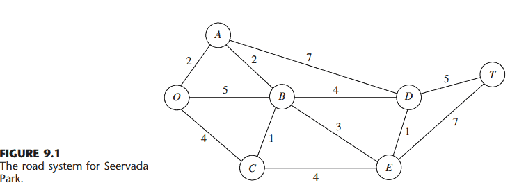
SEERVADA PARK has recently been set aside for a limited amount of sightseeing and backpack hiking. Cars are not allowed into the park, but there is a narrow, winding road system for trams and for jeeps driven by the park rangers. This road system is shown (without the curves) in Fig. 9.1, where location $O$ is the entrance into the park; other letters designate the locations of ranger stations (and other limited facilities). The numbers give the distances of these winding roads in miles.

The park contains a scenic wonder at station $T$. A small number of trams are used to transport sightseers from the park entrance to station $T$ and back.

The park management currently faces three problems. One is to determine which route from the park entrance to station $T$ has the smallest total distance for the operation of the trams. (This is an example of the shortest-path problem to be discussed in Sec. 9.3.)
A second problem is that telephone lines must be installed under the roads to establish telephone communication among all the stations (including the park entrance). Because the installation is both expensive and disruptive to the natural environment, lines will be installed under just enough roads to provide some connection between every pair of stations. The question is where the lines should be laid to accomplish this with a minimum total number of miles of line installed. (This is an example of the minimum spanning tree problem to be discussed in Sec. 9.4.)

The third problem is that more people want to take the tram ride from the park entrance to station $T$ than can be accommodated during the peak season. To avoid unduly disturbing the ecology and wildlife of the region, a strict ration has been placed on the number of tram trips that can be made on each of the roads per day. (These limits differ for the different roads, as we shall describe in detail in Sec. 9.5.) Therefore, during the peak season, various routes might be followed regardless of distance to increase the number of tram trips that can be made each day. The question pertains to how to route the various trips to maximize the number of trips that can be made per day without violating the limits on any individual road. (This is an example of the maximum flow problem to be discussed in Sec. 9.5.)

数学代写|运筹学作业代写operational research代考|THE TERMINOLOGY OF NETWORKS

A relatively extensive terminology has been developed to describe the various kinds of networks and their components. Although we have avoided as much of this special vocabulary as we could, we still need to introduce a considerable number of terms for use throughout the chapter. We suggest that you read through this section once at the outset to understand the definitions and then plan to return to refresh your memory as the terms are used in subsequent sections. To assist you, each term is highlighted in boldface at the point where it is defined.

A network consists of a set of points and a set of lines connecting certain pairs of the points. The points are called nodes (or vertices); e.g., the network in Fig. 9.1 has seven nodes designated by the seven circles. The lines are called arcs (or links or edges or branches); e.g., the network in Fig. 9.1 has 12 arcs corresponding to the 12 roads in the road system. Arcs are labeled by naming the nodes at either end; for example, $A B$ is the $\operatorname{arc}$ between nodes $A$ and $B$ in Fig. 9.1.

The arcs of a network may have a flow of some type through them, e.g., the flow of trams on the roads of Seervada Park in Sec. 9.1. Table 9.1 gives several examples of flow in typical networks. If flow through an arc is allowed in only one direction (e.g., a oneway street), the arc is said to be a directed arc. The direction is indicated by adding an arrowhead at the end of the line representing the arc. When a directed arc is labeled by listing two nodes it connects, the from node always is given before the to node; e.g., an arc that is directed from node $A$ to node $B$ must be labeled as $A B$ rather than $B A$. Alternatively, this arc may be labeled as $A \rightarrow B$.

If flow through an arc is allowed in either direction (e.g., a pipeline that can be used to pump fluid in either direction), the arc is said to be an undirected arc. To help you distinguish between the two kinds of arcs, we shall frequently refer to undirected arcs by the suggestive name of links.

运筹学代考

数学代写|运筹学作业代写operational research代考|PROTOTYPE EXAMPLE

SEERVADA公园最近被划为有限数量的观光和背包徒步旅行。汽车不允许进入公园，但有一条狭窄蜿蜒的道路供有轨电车和公园护林员驾驶的吉普车通行。该道路系统如图9.1所示(没有曲线)，其中位置$O$为进入公园的入口;其他字母标明了护林站(和其他有限设施)的位置。这些数字以英里为单位给出了这些蜿蜒道路的距离。

这个公园在$T$站有一个风景奇观。少量有轨电车用于将游客从公园入口运送到$T$站并返回。

公园管理目前面临三个问题。一是确定哪条路线从公园入口到$T$站的电车运行总距离最小。(这是9.3节将要讨论的最短路径问题的一个例子。)
第二个问题是，必须在道路下安装电话线，以便在所有车站(包括公园入口)之间建立电话通信。由于安装线路既昂贵又破坏自然环境，因此线路将安装在刚好足够的道路下面，以便在每一对车站之间提供一些连接。问题是，为了实现这一目标，应该在哪里铺设这些线路，同时安装的线路总里程最少。(这是最小生成树问题的一个例子，将在第9.4节讨论。)

第三个问题是，更多的人想乘坐有轨电车从公园入口到T站，而不是在旺季容纳。为了避免对该地区的生态和野生动物造成过度的干扰，每天每条道路上的电车班次都有严格的限制。(这些限制因道路不同而不同，我们将在第9.5节详细描述。)因此，在高峰季节，无论距离远近，都可以选择不同的路线，以增加每天的有轨电车班次。这个问题是关于如何在不违反任何一条道路的限制的情况下，将各种旅行路线安排到每天可以进行的旅行数量最大化。(这是9.5节将讨论的最大流量问题的一个例子。)

数学代写|运筹学作业代写operational research代考|THE TERMINOLOGY OF NETWORKS

已经发展了一个相对广泛的术语来描述各种网络及其组成部分。尽管我们已经尽可能避免使用这些特殊词汇，但我们仍然需要在本章中介绍相当数量的术语。我们建议您在开始时通读一遍本节以理解定义，然后计划在后续章节中使用这些术语时返回来刷新您的记忆。为了帮助您，每个术语在定义处都以黑体字突出显示。

网络由一组点和一组连接点对的线组成。这些点被称为节点(或顶点);例如，图9.1中的网络有七个节点，由七个圆圈表示。这些线被称为弧(或链接、边或分支);例如，图9.1中的网络有12个圆弧，对应道路系统中的12条道路。通过命名两端的节点来标记弧;例如，$A B$是图9.1中$A$和$B$之间的$\operatorname{arc}$。

网络的弧线可能有某种类型的流通过它们，例如第9.1节中Seervada公园道路上的有轨电车流。表9.1给出了几个典型网络中的流程示例。如果气流只允许从一个方向流过一个弧(例如，单行道)，则称该弧为有向弧。方向是通过在代表圆弧的线的末端添加一个箭头来指示的。当有向弧通过列出它所连接的两个节点来标记时，从节点总是在到节点之前给出;例如，从节点$A$指向节点$B$的弧线必须标记为$A B$而不是$B A$。或者，这条弧可以标记为$A \右转B$。

如果允许沿任一方向流过弧(例如，可用于向任一方向泵送流体的管道)，则称该弧为无向弧。为了帮助您区分这两种类型的弧，我们将经常通过链接的暗示性名称来提及无向弧。

统计代写|运筹学作业代写operational research代考请认准statistics-lab™

统计代写请认准statistics-lab™. statistics-lab™为您的留学生涯保驾护航。

金融工程代写

金融工程是使用数学技术来解决金融问题。金融工程使用计算机科学、统计学、经济学和应用数学领域的工具和知识来解决当前的金融问题，以及设计新的和创新的金融产品。

非参数统计代写

非参数统计指的是一种统计方法，其中不假设数据来自于由少数参数决定的规定模型；这种模型的例子包括正态分布模型和线性回归模型。

广义线性模型代考

广义线性模型（GLM）归属统计学领域，是一种应用灵活的线性回归模型。该模型允许因变量的偏差分布有除了正态分布之外的其它分布。

术语广义线性模型（GLM）通常是指给定连续和/或分类预测因素的连续响应变量的常规线性回归模型。它包括多元线性回归，以及方差分析和方差分析（仅含固定效应）。

有限元方法代写

有限元方法（FEM）是一种流行的方法，用于数值解决工程和数学建模中出现的微分方程。典型的问题领域包括结构分析、传热、流体流动、质量运输和电磁势等传统领域。

有限元是一种通用的数值方法，用于解决两个或三个空间变量的偏微分方程（即一些边界值问题）。为了解决一个问题，有限元将一个大系统细分为更小、更简单的部分，称为有限元。这是通过在空间维度上的特定空间离散化来实现的，它是通过构建对象的网格来实现的：用于求解的数值域，它有有限数量的点。边界值问题的有限元方法表述最终导致一个代数方程组。该方法在域上对未知函数进行逼近。[1] 然后将模拟这些有限元的简单方程组合成一个更大的方程系统，以模拟整个问题。然后，有限元通过变化微积分使相关的误差函数最小化来逼近一个解决方案。

tatistics-lab作为专业的留学生服务机构，多年来已为美国、英国、加拿大、澳洲等留学热门地的学生提供专业的学术服务，包括但不限于Essay代写，Assignment代写，Dissertation代写，Report代写，小组作业代写，Proposal代写，Paper代写，Presentation代写，计算机作业代写，论文修改和润色，网课代做，exam代考等等。写作范围涵盖高中，本科，研究生等海外留学全阶段，辐射金融，经济学，会计学，审计学，管理学等全球99%专业科目。写作团队既有专业英语母语作者，也有海外名校硕博留学生，每位写作老师都拥有过硬的语言能力，专业的学科背景和学术写作经验。我们承诺100%原创，100%专业，100%准时，100%满意。

随机分析代写

随机微积分是数学的一个分支，对随机过程进行操作。它允许为随机过程的积分定义一个关于随机过程的一致的积分理论。这个领域是由日本数学家伊藤清在第二次世界大战期间创建并开始的。

时间序列分析代写

随机过程，是依赖于参数的一组随机变量的全体，参数通常是时间。随机变量是随机现象的数量表现，其时间序列是一组按照时间发生先后顺序进行排列的数据点序列。通常一组时间序列的时间间隔为一恒定值（如1秒，5分钟，12小时，7天，1年），因此时间序列可以作为离散时间数据进行分析处理。研究时间序列数据的意义在于现实中，往往需要研究某个事物其随时间发展变化的规律。这就需要通过研究该事物过去发展的历史记录，以得到其自身发展的规律。

回归分析代写

多元回归分析渐进（Multiple Regression Analysis Asymptotics）属于计量经济学领域，主要是一种数学上的统计分析方法，可以分析复杂情况下各影响因素的数学关系，在自然科学、社会和经济学等多个领域内应用广泛。

MATLAB代写

MATLAB 是一种用于技术计算的高性能语言。它将计算、可视化和编程集成在一个易于使用的环境中，其中问题和解决方案以熟悉的数学符号表示。典型用途包括：数学和计算算法开发建模、仿真和原型制作数据分析、探索和可视化科学和工程图形应用程序开发，包括图形用户界面构建MATLAB 是一个交互式系统，其基本数据元素是一个不需要维度的数组。这使您可以解决许多技术计算问题，尤其是那些具有矩阵和向量公式的问题，而只需用 C 或 Fortran 等标量非交互式语言编写程序所需的时间的一小部分。MATLAB 名称代表矩阵实验室。MATLAB 最初的编写目的是提供对由 LINPACK 和 EISPACK 项目开发的矩阵软件的轻松访问，这两个项目共同代表了矩阵计算软件的最新技术。MATLAB 经过多年的发展，得到了许多用户的投入。在大学环境中，它是数学、工程和科学入门和高级课程的标准教学工具。在工业领域，MATLAB 是高效研究、开发和分析的首选工具。MATLAB 具有一系列称为工具箱的特定于应用程序的解决方案。对于大多数 MATLAB 用户来说非常重要，工具箱允许您学习和应用专业技术。工具箱是 MATLAB 函数（M 文件）的综合集合，可扩展 MATLAB 环境以解决特定类别的问题。可用工具箱的领域包括信号处理、控制系统、神经网络、模糊逻辑、小波、仿真等。

R语言代写	问卷设计与分析代写
PYTHON代写	回归分析与线性模型代写
MATLAB代写	方差分析与试验设计代写
STATA代写	机器学习/统计学习代写
SPSS代写	计量经济学代写
EVIEWS代写	时间序列分析代写
EXCEL代写	深度学习代写
SQL代写	各种数据建模与可视化代写

数学代写|运筹学作业代写operational research代考|THE TRANSPORTATION PROBLEM

Posted on 2023年7月7日2023年7月7日 by statistics-lab

数学代写|运筹学作业代写operational research代考|THE TRANSPORTATION PROBLEM

One of the main products of the P \& T COMPANY is canned peas. The peas are prepared at three canneries (near Bellingham, Washington; Eugene, Oregon; and Albert Lea, Minnesota) and then shipped by truck to four distributing warehouses in the western United States (Sacramento, California; Salt Lake City, Utah; Rapid City, South Dakota; and Albuquerque, New Mexico), as shown in Fig. 8.1. Because the shipping costs are a major expense, management is initiating a study to reduce them as much as possible. For the upcoming season, an estimate has been made of the output from each cannery, and each warehouse has been allocated a certain amount from the total supply of peas. This information (in units of truckloads), along with the shipping cost per truckload for each cannery-warehouse combination, is given in Table 8.2. Thus, there are a total of 300 truckloads to be shipped. The problem now is to determine which plan for assigning these shipments to the various cannery-warehouse combinations would minimize the total shipping cost.

By ignoring the geographical layout of the canneries and warehouses, we can provide a network representation of this problem in a simple way by lining up all the canneries in one column on the left and all the warehouses in one column on the right. This representation is shown in Fig. 8.2. The arrows show the possible routes for the truckloads, where the number next to each arrow is the shipping cost per truckload for that route. A square bracket next to each location gives the number of truckloads to be shipped out of that location (so that the allocation into each warehouse is given as a negative number).

The problem depicted in Fig. 8.2 is actually a linear programming problem of the transportation problem type. To formulate the model, let $Z$ denote total shipping cost, and let $x_{i j}(i=1,2,3 ; j=1,2,3,4)$ be the number of truckloads to be shipped from cannery $i$ to warehouse $j$. Thus, the objective is to choose the values of these 12 decision variables (the $x_{i j}$ ) so as to
$$
\begin{aligned}
& \text { Minimize } Z=464 x_{11}+513 x_{12}+654 x_{13}+867 x_{14}+352 x_{21}+416 x_{22} \
& +690 x_{23}+791 x_{24}+995 x_{31}+682 x_{32}+388 x_{33}+685 x_{34}, \
&
\end{aligned}
$$

数学代写|运筹学作业代写operational research代考|An Award Winning Application of a Transportation Problem

Except for its small size, the P \& T Co. problem is typical of the problems faced by many corporations which must ship goods from their manufacturing plants to their customers.
For example, consider an award winning OR study conducted at Proctor \& Gamble (as described in the January-February 1997 issue of Interfaces). Prior to the study, the company’s supply chain consisted of hundreds of suppliers, over 50 product categories, over 60 plants, 15 distribution centers, and over 1,000 customer zones. However, as the company moved toward global brands, management realized that it needed to consolidate plants to reduce manufacturing expenses, improve speed to market, and reduce capital investment. Therefore, the study focused on redesigning the company’s production and distribution system for its North American operations. The result was a reduction in the number of North American plants by almost 20 percent, saving over $\$ 200$ million in pretax costs per year.

A major part of the study revolved around formulating and solving transportation problems for individual product categories. For each option regarding the plants to keep open, etc., solving the corresponding transportation problem for a product category shows what the distribution cost would be for shipping the product category from those plants to the distribution centers and customer zones. Numerous such transportation problems were solved in the process of identifying the best new production and distribution system.

运筹学代考

数学代写|运筹学作业代写operational research代考|THE TRANSPORTATION PROBLEM

P ＆ T公司的主要产品之一是罐装豌豆。豌豆是在三个罐头厂(华盛顿州贝灵汉附近;俄勒冈州尤金;和Albert Lea，明尼苏达州)，然后用卡车运到美国西部的四个配送仓库(加利福尼亚州萨克拉门托;犹他州盐湖城;拉皮德城，南达科他州;和新墨西哥州阿尔伯克基)，如图8.1所示。由于运输费用是一项主要开支，管理部门正在着手研究如何尽可能地减少运输费用。对于即将到来的季节，已经对每个罐头厂的产量进行了估计，并且每个仓库从豌豆的总供应量中分配了一定的数量。表8.2给出了这些信息(以卡车为单位)，以及每个罐头厂-仓库组合的每卡车运输成本。因此，总共有300辆卡车要装运。现在的问题是确定将这些货物分配到各种罐头厂-仓库组合的哪个计划将使总运输成本最小化。

通过忽略罐头厂和仓库的地理布局，我们可以以一种简单的方式提供这个问题的网络表示:将所有罐头厂排在左边一列，将所有仓库排在右边一列。这种表示如图8.2所示。箭头显示了卡车可能的运输路线，每个箭头旁边的数字是该路线上每辆卡车的运输成本。每个位置旁边的方括号给出了要从该位置运出的卡车数量(因此每个仓库的分配以负数给出)。

图8.2所描述的问题实际上是运输问题类型的线性规划问题。为建立模型，设$Z$表示总运输成本，设$x_{i j}(i=1,2,3 ; j=1,2,3,4)$为从罐头厂$i$运送到仓库$j$的卡车数量。因此，目标是选择这12个决策变量($x_{i j}$)的值，以便
$$
\begin{aligned}
& \text { Minimize } Z=464 x_{11}+513 x_{12}+654 x_{13}+867 x_{14}+352 x_{21}+416 x_{22} \
& +690 x_{23}+791 x_{24}+995 x_{31}+682 x_{32}+388 x_{33}+685 x_{34}, \
&
\end{aligned}
$$

数学代写|运筹学作业代写operational research代考|An Award Winning Application of a Transportation Problem

除了规模小之外，宝洁公司的问题是许多公司所面临的典型问题，这些公司必须把货物从制造工厂运送到客户那里。
例如，考虑在Proctor ＆ Gamble进行的获奖OR研究(如1997年1 – 2月的《界面》所述)。在研究之前，该公司的供应链由数百家供应商、50多个产品类别、60多个工厂、15个配送中心和1000多个客户区组成。然而，随着公司走向全球品牌，管理层意识到需要整合工厂，以减少制造费用，提高上市速度，并减少资本投资。因此，研究的重点是重新设计公司的生产和分销系统，为其北美业务。结果是北美工厂的数量减少了近20％，每年节省了超过$\$ 200$万美元的税前成本。

研究的一个主要部分是围绕制定和解决个别产品类别的运输问题。对于关于工厂保持开放等的每个选项，解决产品类别的相应运输问题将显示将产品类别从这些工厂运输到配送中心和客户区域的配送成本。在确定最佳的新生产和分配系统的过程中，解决了许多这样的运输问题。

统计代写请认准statistics-lab™. statistics-lab™为您的留学生涯保驾护航。

金融工程代写

非参数统计代写

非参数统计指的是一种统计方法，其中不假设数据来自于由少数参数决定的规定模型；这种模型的例子包括正态分布模型和线性回归模型。

广义线性模型代考

广义线性模型（GLM）归属统计学领域，是一种应用灵活的线性回归模型。该模型允许因变量的偏差分布有除了正态分布之外的其它分布。

有限元方法代写

随机分析代写

时间序列分析代写

回归分析代写

MATLAB代写

R语言代写	问卷设计与分析代写
PYTHON代写	回归分析与线性模型代写
MATLAB代写	方差分析与试验设计代写
STATA代写	机器学习/统计学习代写
SPSS代写	计量经济学代写
EVIEWS代写	时间序列分析代写
EXCEL代写	深度学习代写
SQL代写	各种数据建模与可视化代写

数学代写|运筹学作业代写operational research代考|The Relevance of the Gradient for Concepts 1 and 2

Posted on 2023年7月7日2023年7月7日 by statistics-lab

数学代写|运筹学作业代写operational research代考|The Relevance of the Gradient for Concepts 1 and 2

The algorithm begins with an initial trial solution that (like all subsequent trial solutions) lies in the interior of the feasible region, i.e., inside the boundary of the feasible region. Thus, for the example, the solution must not lie on any of the three lines $\left(x_1=0, x_2=0\right.$, $x_1+x_2=8$ ) that form the boundary of this region in Fig. 7.3. (A trial solution that lies on the boundary cannot be used because this would lead to the undefined mathematical operation of division by zero at one point in the algorithm.) We have arbitrarily chosen $\left(x_1, x_2\right)=(2,2)$ to be the initial trial solution.

To begin implementing concepts 1 and 2, note in Fig. 7.3 that the direction of movement from $(2,2)$ that increases $Z$ at the fastest possible rate is perpendicular to (and toward) the objective function line $Z=16=x_1+2 x_2$. We have shown this direction by the arrow from $(2,2)$ to $(3,4)$. Using vector addition, we have
$$
(3,4)=(2,2)+(1,2),
$$
where the vector $(1,2)$ is the gradient of the objective function. (We will discuss gradients further in Sec. 13.5 in the broader context of nonlinear programming, where algorithms similar to Karmarkar’s have long been used.) The components of $(1,2)$ are just the coefficients in the objective function. Thus, with one subsequent modification, the gradient $(1,2)$ defines the ideal direction to which to move, where the question of the distance to move will be considered later.

The algorithm actually operates on linear programming problems after they have been rewritten in augmented form. Letting $x_3$ be the slack variable for the functional constraint of the example, we see that this form is
$$
\text { Maximize } Z=x_1+2 x_2 \text {, }
$$
subject to
$$
x_1+x_2+x_3=8
$$
and
$$
x_1 \geq 0, \quad x_2 \geq 0, \quad x_3 \geq 0 .
$$
In matrix notation (slightly different from Chap. 5 because the slack variable now is incorporated into the notation), the augmented form can be written in general as
$$
\begin{aligned}
& \text { Maximize } Z=\mathbf{c}^T \mathbf{x}, \
& \text { subject to } \
& \mathbf{A x}=\mathbf{b}
\end{aligned}
$$
and
$$
\mathbf{x} \geq \mathbf{0},
$$
where
$$
\mathbf{c}=\left[\begin{array}{l}
1 \
2 \
0
\end{array}\right], \quad \mathbf{x}=\left[\begin{array}{l}
x_1 \
x_2 \
x_3
\end{array}\right], \quad \mathbf{A}=\left[\begin{array}{lll}
1, & 1, & 1
\end{array}\right], \quad \mathbf{b}=[8], \quad \mathbf{0}=\left[\begin{array}{l}
0 \
0 \
0
\end{array}\right]
$$
for the example. Note that $\mathbf{c}^T=[1,2,0]$ now is the gradient of the objective function.

数学代写|运筹学作业代写operational research代考|Using the Projected Gradient to Implement Concepts 1 and 2

In augmented form, the initial trial solution for the example is $\left(x_1, x_2, x_3\right)=(2,2,4)$. Adding the gradient $(1,2,0)$ leads to
$$
(3,4,4)=(2,2,4)+(1,2,0)
$$
However, now there is a complication. The algorithm cannot move from $(2,2,4)$ toward $(3,4,4)$, because $(3,4,4)$ is infeasible! When $x_1=3$ and $x_2=4$, then $x_3=8-x_1-$ $x_2=1$ instead of 4 . The point $(3,4,4)$ lies on the near side as you look down on the feasible triangle in Fig. 7.4. Therefore, to remain feasible, the algorithm (indirectly) projects the point $(3,4,4)$ down onto the feasible triangle by dropping a line that is perpendicular to this triangle. A vector from $(0,0,0)$ to $(1,1,1)$ is perpendicular to this triangle, so the perpendicular line through $(3,4,4)$ is given by the equation
$$
\left(x_1, x_2, x_3\right)=(3,4,4)-\theta(1,1,1) \text {, }
$$
where $\theta$ is a scalar. Since the triangle satisfies the equation $x_1+x_2+x_3=8$, this perpendicular line intersects the triangle at $(2,3,3)$. Because
$$
(2,3,3)=(2,2,4)+(0,1,-1),
$$
the projected gradient of the objective function (the gradient projected onto the feasible region) is $(0,1,-1)$. It is this projected gradient that defines the direction of movement for the algorithm, as shown by the arrow in Fig. 7.4.

A formula is available for computing the projected gradient directly. By defining the projection matrix $\mathbf{P}$ as
$$
\mathbf{P}=\mathbf{I}-\mathbf{A}^T\left(\mathbf{A} \mathbf{A}^T\right)^{-1} \mathbf{A},
$$
the projected gradient (in column form) is
$$
\mathbf{c}_p=\mathbf{P c} .
$$

运筹学代考

数学代写|运筹学作业代写operational research代考|The Relevance of the Gradient for Concepts 1 and 2

该算法从一个初始试解开始，该初始试解(像所有后续的试解一样)位于可行域的内部，即在可行域的边界内。因此，例如，解不得位于图7.3中形成该区域边界的三条线$\left(x_1=0, x_2=0\right.$, $x_1+x_2=8$中的任何一条线上。(不能使用位于边界上的试解，因为这将导致算法中某一点被零除的未定义数学操作。)我们任意选择$\left(x_1, x_2\right)=(2,2)$作为初始试解。

为了开始实现概念1和2，请注意图7.3中从$(2,2)$开始以最快的速度增加$Z$的运动方向垂直于(并朝向)目标函数线$Z=16=x_1+2 x_2$。我们用从$(2,2)$到$(3,4)$的箭头表示了这个方向。用向量加法，我们有
$$
(3,4)=(2,2)+(1,2),
$$
其中向量$(1,2)$是目标函数的梯度。(我们将在13.5节中在更广泛的非线性规划背景下进一步讨论梯度，在非线性规划中，类似Karmarkar的算法早已被使用。)$(1,2)$的分量就是目标函数的系数。因此，通过一个后续修改，梯度$(1,2)$定义了移动的理想方向，其中移动距离的问题将在稍后考虑。

该算法实际上是在线性规划问题被改写成增广形式后运行的。设$x_3$为本例函数约束的松弛变量，我们看到这种形式是
$$
\text { Maximize } Z=x_1+2 x_2 \text {, }
$$
以
$$
x_1+x_2+x_3=8
$$
和
$$
x_1 \geq 0, \quad x_2 \geq 0, \quad x_3 \geq 0 .
$$
在矩阵表示法中(与第5章略有不同，因为松弛变量现在被合并到表示法中)，增广形式通常可以写成
$$
\begin{aligned}
& \text { Maximize } Z=\mathbf{c}^T \mathbf{x}, \
& \text { subject to } \
& \mathbf{A x}=\mathbf{b}
\end{aligned}
$$
和
$$
\mathbf{x} \geq \mathbf{0},
$$
在哪里
$$
\mathbf{c}=\left[\begin{array}{l}
1 \
2 \
0
\end{array}\right], \quad \mathbf{x}=\left[\begin{array}{l}
x_1 \
x_2 \
x_3
\end{array}\right], \quad \mathbf{A}=\left[\begin{array}{lll}
1, & 1, & 1
\end{array}\right], \quad \mathbf{b}=[8], \quad \mathbf{0}=\left[\begin{array}{l}
0 \
0 \
0
\end{array}\right]
$$
举个例子。注意$\mathbf{c}^T=[1,2,0]$现在是目标函数的梯度。

数学代写|运筹学作业代写operational research代考|Using the Projected Gradient to Implement Concepts 1 and 2

在增广形式中，该示例的初始试验解为$\left(x_1, x_2, x_3\right)=(2,2,4)$。添加渐变$(1,2,0)$导致
$$
(3,4,4)=(2,2,4)+(1,2,0)
$$
然而，现在有一个复杂的问题。算法不能从$(2,2,4)$移动到$(3,4,4)$，因为$(3,4,4)$是不可行的!当$x_1=3$和$x_2=4$时，则$x_3=8-x_1-$$x_2=1$而不是4。当你向下看图7.4中的可行三角形时，点$(3,4,4)$位于近侧。因此，为了保持可行，该算法(间接地)将点$(3,4,4)$投影到可行三角形上，方法是将一条垂直于可行三角形的直线向下投影。一个从$(0,0,0)$到$(1,1,1)$的向量垂直于这个三角形，所以通过$(3,4,4)$的垂直线由这个方程给出
$$
\left(x_1, x_2, x_3\right)=(3,4,4)-\theta(1,1,1) \text {, }
$$
其中$\theta$是标量。因为三角形满足方程$x_1+x_2+x_3=8$，所以这条垂线与三角形相交于$(2,3,3)$。因为
$$
(2,3,3)=(2,2,4)+(0,1,-1),
$$
目标函数的投影梯度(投影到可行区域上的梯度)为$(0,1,-1)$。正是这个投影梯度定义了算法的移动方向，如图7.4中的箭头所示。

给出了直接计算投影梯度的公式。通过定义投影矩阵$\mathbf{P}$为
$$
\mathbf{P}=\mathbf{I}-\mathbf{A}^T\left(\mathbf{A} \mathbf{A}^T\right)^{-1} \mathbf{A},
$$
投影梯度(以列形式)为
$$
\mathbf{c}_p=\mathbf{P c} .
$$

统计代写请认准statistics-lab™. statistics-lab™为您的留学生涯保驾护航。

金融工程代写

非参数统计代写

非参数统计指的是一种统计方法，其中不假设数据来自于由少数参数决定的规定模型；这种模型的例子包括正态分布模型和线性回归模型。

广义线性模型代考

广义线性模型（GLM）归属统计学领域，是一种应用灵活的线性回归模型。该模型允许因变量的偏差分布有除了正态分布之外的其它分布。

有限元方法代写

随机分析代写

时间序列分析代写

回归分析代写

MATLAB代写

R语言代写	问卷设计与分析代写
PYTHON代写	回归分析与线性模型代写
MATLAB代写	方差分析与试验设计代写
STATA代写	机器学习/统计学习代写
SPSS代写	计量经济学代写
EVIEWS代写	时间序列分析代写
EXCEL代写	深度学习代写
SQL代写	各种数据建模与可视化代写

数学代写|运筹学作业代写operational research代考|Case 2a—Changes in the Coefficients of a Nonbasic Variable

Posted on 2023年6月19日2023年6月19日 by statistics-lab

数学代写|运筹学作业代写operational research代考|Case 2a—Changes in the Coefficients of a Nonbasic Variable

Consider a particular variable $x_j$ (fixed $j$ ) that is a nonbasic variable in the optimal solution shown by the final simplex tableau. In Case $2 a$, the only change in the current model is that one or more of the coefficients of this variable $-c_j, a_{1 j}, a_{2 j}, \ldots, a_{m j}$-have been changed. Thus, letting $\bar{c}j$ and $\bar{a}{i j}$ denote the new values of these parameters, with $\overline{\mathbf{A}}j$ (column $j$ of matrix $\overline{\mathbf{A}}$ ) as the vector containing the $\bar{a}{i j}$, we have
$$
c_j \longrightarrow \bar{c}_j, \quad \mathbf{A}_j \longrightarrow \overline{\mathbf{A}}_j
$$
for the revised model.
As described at the beginning of Sec. 6.5, duality theory provides a very convenient way of checking these changes. In particular, if the complementary basic solution $\mathbf{y}^$ in the dual problem still satisfies the single dual constraint that has changed, then the original optimal solution in the primal problem remains optimal as is. Conversely, if $\mathbf{y}^$ violates this dual constraint, then this primal solution is no longer optimal.

If the optimal solution has changed and you wish to find the new one, you can do so rather easily. Simply apply the fundamental insight to revise the $x_j$ column (the only one that has changed) in the final simplex tableau. Specifically, the formulas in Table 6.17 reduce to the following:
Coefficient of $x_j$ in final row 0 :
Coefficient of $x_j$ in final rows 1 to $m$ :
$$
\begin{aligned}
& z_j^-\bar{c}_j=\mathbf{y}^ \overline{\mathbf{A}}_j-\bar{c}_j, \
& \mathbf{A}_j^*=\mathbf{S} * \overline{\mathbf{A}}_j .
\end{aligned}
$$
With the current basic solution no longer optimal, the new value of $z_j^*-c_j$ now will be the one negative coefficient in row 0 , so restart the simplex method with $x_j$ as the initial entering basic variable.

Note that this procedure is a streamlined version of the general procedure summarized at the end of Sec. 6.6. Steps 3 and 4 (conversion to proper form from Gaussian elimination and the feasibility test) have been deleted as irrelevant, because the only column being changed in the revision of the final tableau (before reoptimization) is for the nonbasic variable $x_j$. Step 5 (optimality test) has been replaced by a quicker test of optimality to be performed right after step 1 (revision of model). It is only if this test reveals that the optimal solution has changed, and you wish to find the new one, that steps 2 and 6 (revision of final tableau and reoptimization) are needed.

数学代写|运筹学作业代写operational research代考|Analyzing Simultaneous Changes in Objective Function Coefficients

Analyzing Simultaneous Changes in Objective Function Coefficients. Regardless of whether $x_j$ is a basic or nonbasic variable, the allowable range to stay optimal for $c_j$ is valid only if this objective function coefficient is the only one being changed. However, when simultaneous changes are made in the coefficients of the objective function, a 100 percent rule is available for checking whether the original solution must still be optimal. Much like the 100 percent rule for simultaneous changes in right-hand sides, this 100 percent rule combines the allowable changes (increase or decrease) for the individual $c_j$ that are given by the last two columns of a table like Table 6.23, as described below.
The 100 Percent Rule for Simultaneous Changes in Objective Function Coefficients: If simultaneous changes are made in the coefficients of the objective function, calculate for each change the percentage of the allowable change (increase or decrease) for that coefficient to remain within its allowable range to stay optimal. If the sum of the percentage changes does not exceed 100 percent, the original optimal solution definitely will still be optimal. (If the sum does exceed 100 percent, then we cannot be sure.)
Using Table 6.23 (and referring to Fig. 6.3 for visualization), this 100 percent rule says that $(0,9)$ will remain optimal for Variation 2 of the Wyndor Glass Co. model even if we simultaneously increase $c_1$ from 3 and decrease $c_2$ from 5 as long as these changes are not too large. For example, if $c_1$ is increased by 1.5 (33 $\frac{1}{3}$ percent of the allowable change), then $c_2$ can be decreased by as much as 2 (66 $\frac{2}{2}$ percent of the allowable change). Similarly, if $c_1$ is increased by 3 (66 $\frac{2}{3}$ percent of the allowable change), then $c_2$ can only changes revise the objective function to either $Z=4.5 x_1+3 x_2$ or $Z=6 x_1+4 x_2$, which causes the optimal objective function line in Fig. 6.3 to rotate clockwise until it coincides with the constraint boundary equation $3 x_1+2 x_2=18$.

运筹学代考

数学代写|运筹学作业代写operational research代考|Case 2a—Changes in the Coefficients of a Nonbasic Variable

考虑一个特定的变量$x_j$(固定的$j$)，它是最终单纯形表所示的最优解中的一个非基本变量。在情况$2 a$中，当前模型的唯一变化是该变量$-c_j, a_{1 j}, a_{2 j}, \ldots, a_{m j}$ -的一个或多个系数已被更改。因此，让$\bar{c}j$和$\bar{a}{i j}$表示这些参数的新值，用$\overline{\mathbf{A}}j$(矩阵$\overline{\mathbf{A}}$的$j$列)作为包含$\bar{a}{i j}$的向量，我们得到
$$
c_j \longrightarrow \bar{c}_j, \quad \mathbf{A}_j \longrightarrow \overline{\mathbf{A}}_j
$$
修改后的模型。
正如第6.5节开头所描述的，对偶理论提供了一种非常方便的检查这些更改的方法。特别是，如果对偶问题的互补基本解$\mathbf{y}^$仍然满足改变后的单对偶约束，则原始问题的原最优解仍然是最优解。相反，如果$\mathbf{y}^$违反了这个双重约束，那么这个原始解就不再是最优的。

如果最优解发生了变化，而您希望找到新的解，那么您可以很容易地做到这一点。只需应用基本见解来修改最终simplex表中的$x_j$列(唯一更改的列)。具体来说，表6.17中的公式可以简化为:
最后第0行$x_j$系数:
最后1 ～ $m$中$x_j$的系数:
$$
\begin{aligned}
& z_j^-\bar{c}_j=\mathbf{y}^ \overline{\mathbf{A}}_j-\bar{c}_j, \
& \mathbf{A}_j^*=\mathbf{S} * \overline{\mathbf{A}}_j .
\end{aligned}
$$
由于当前基本解不再是最优的，$z_j^*-c_j$的新值现在将是第0行中的一个负系数，因此重新启动单纯形方法，将$x_j$作为初始输入基本变量。

注意，这个过程是第6.6节末尾总结的一般过程的精简版本。步骤3和4(从高斯消去和可行性测试转换为适当形式)已被删除，因为在最终表的修订中(在重新优化之前)唯一更改的列是用于非基本变量$x_j$。第5步(最优性测试)已经被第1步(模型修正)之后执行的更快速的最优性测试所取代。只有当这个测试表明最优解发生了变化，而您希望找到新的解决方案时，才需要第2步和第6步(修改最终表格和重新优化)。

数学代写|运筹学作业代写operational research代考|Analyzing Simultaneous Changes in Objective Function Coefficients

分析目标函数系数的同步变化。无论$x_j$是基本变量还是非基本变量，只有当目标函数系数是唯一被改变的变量时，$c_j$保持最优的允许范围才有效。然而，当目标函数的系数同时发生变化时，可以使用100％规则来检查原始解决方案是否必须仍然是最优的。与右侧同时更改的100％规则非常相似，这个100％规则结合了表(如表6.23)的最后两列给出的单个$c_j$的允许更改(增加或减少)，如下所述。
目标函数系数同时变化100％规则:如果目标函数的系数同时发生变化，则计算每次变化允许变化(增加或减少)的百分比，使该系数保持在其允许范围内以保持最佳状态。如果百分比变化的总和不超过100％，那么原始的最优解肯定仍然是最优的。(如果总数确实超过100％，那么我们就不能确定。)
使用表6.23(并参考图6.3进行可视化)，这个100％规则表明$(0,9)$对于Wyndor Glass Co.模型的变体2仍然是最优的，即使我们同时从3增加$c_1$并从5减少$c_2$，只要这些变化不是太大。例如，如果$c_1$增加1.5(占允许变化的33％ $\frac{1}{3}$ ％)，那么$c_2$可以减少2(占允许变化的66％ $\frac{2}{2}$ ％)。同样，如果$c_1$增加3 (66.$\frac{2}{3}$ ％的允许变化)，则$c_2$只能将目标函数修改为$Z=4.5 x_1+3 x_2$或$Z=6 x_1+4 x_2$，从而导致图6.3中最优目标函数线顺时针旋转，直到与约束边界方程$3 x_1+2 x_2=18$重合。

统计代写请认准statistics-lab™. statistics-lab™为您的留学生涯保驾护航。

金融工程代写

非参数统计代写

非参数统计指的是一种统计方法，其中不假设数据来自于由少数参数决定的规定模型；这种模型的例子包括正态分布模型和线性回归模型。

广义线性模型代考

广义线性模型（GLM）归属统计学领域，是一种应用灵活的线性回归模型。该模型允许因变量的偏差分布有除了正态分布之外的其它分布。

有限元方法代写

随机分析代写

时间序列分析代写

回归分析代写

MATLAB代写

R语言代写	问卷设计与分析代写
PYTHON代写	回归分析与线性模型代写
MATLAB代写	方差分析与试验设计代写
STATA代写	机器学习/统计学习代写
SPSS代写	计量经济学代写
EVIEWS代写	时间序列分析代写
EXCEL代写	深度学习代写
SQL代写	各种数据建模与可视化代写

数学代写|运筹学作业代写operational research代考|Interpretation of the Dual Problem

Posted on 2023年6月19日2023年6月19日 by statistics-lab

数学代写|运筹学作业代写operational research代考|Interpretation of the Dual Problem

To see how this interpretation of the primal problem leads to an economic interpretation for the dual problem, ${ }^1$ note in Table 6.4 that $W$ is the value of $Z$ (total profit) at the current iteration. Because
$$
W=b_1 y_1+b_2 y_2+\cdots+b_m y_m
$$
each $b_i y_i$ can thereby be interpreted as the current contribution to profit by having $b_i$ units of resource $i$ available for the primal problem. Thus,
The dual variable $y_i$ is interpreted as the contribution to profit per unit of resource $i$ $(i=1,2, \ldots, m)$, when the current set of basic variables is used to obtain the primal solution.
In other words, the $y_i$ values (or $y_i^*$ values in the optimal solution) are just the shadow prices discussed in Sec. 4.7.

For example, when iteration 2 of the simplex method finds the optimal solution for the Wyndor problem, it also finds the optimal values of the dual variables (as shown in the bottom row of Table 6.5) to be $y_1^=0, y_2^=\frac{3}{2}$, and $y_3^=1$. These are precisely the shadow prices found in Sec. 4.7 for this problem through graphical analysis. Recall that the resources for the Wyndor problem are the production capacities of the three plants being made available to the two new products under consideration, so that $b_i$ is the number of hours of production time per week being made available in Plant $i$ for these new products, where $i=1,2,3$. As discussed in Sec. 4.7, the shadow prices indicate that individually increasing any $b_i$ by 1 would increase the optimal value of the objective function (total weekly profit in units of thousands of dollars) by $y_i^$. Thus, $y_i^*$ can be interpreted as the contribution to profit per unit of resource $i$ when using the optimal solution.

数学代写|运筹学作业代写operational research代考|Interpretation of the Simplex Method

The interpretation of the dual problem also provides an economic interpretation of what the simplex method does in the primal problem. The goal of the simplex method is to find how to use the available resources in the most profitable feasible way. To attain this goal, we must reach a $\mathrm{BF}$ solution that satisfies all the requirements on profitable use of the resources (the constraints of the dual problem). These requirements comprise the condition for optimality for the algorithm. For any given BF solution, the requirements (dual constraints) associated with the basic variables are automatically satisfied (with equality). However, those associated with nonbasic variables may or may not be satisfied.

In particular, if an original variable $x_j$ is nonbasic so that activity $j$ is not used, then the current contribution to profit of the resources that would be required to undertake each unit of activity $j$
$$
\sum_{i=1}^m a_{i j} y_i
$$
may be smaller than, larger than, or equal to the unit profit $c_j$ obtainable from the activity. If it is smaller, so that $z_j-c_j<0$ in row 0 of the simplex tableau, then these resources can be used more profitably by initiating this activity. If it is larger $\left(z_j-c_j>0\right)$, then these resources already are being assigned elsewhere in a more profitable way, so they should not be diverted to activity $j$. If $z_j-c_j=0$, there would be no change in profitability by initiating activity $j$.

Similarly, if a slack variable $x_{n+i}$ is nonbasic so that the total allocation $b_i$ of resource $i$ is being used, then $y_i$ is the current contribution to profit of this resource on a marginal basis. Hence, if $y_i<0$, profit can be increased by cutting back on the use of this resource (i.e., increasing $x_{n+i}$ ). If $y_i>0$, it is worthwhile to continue fully using this resource, whereas this decision does not affect profitability if $y_i=0$.

运筹学代考

数学代写|运筹学作业代写operational research代考|Interpretation of the Dual Problem

为了了解这种对原始问题的解释如何导致对偶问题的经济解释，${ }^1$请注意表6.4中$W$是当前迭代中$Z$(总利润)的值。因为
$$
W=b_1 y_1+b_2 y_2+\cdots+b_m y_m
$$
因此，每个$b_i y_i$都可以被解释为当前对利润的贡献，因为原始问题有$b_i$单位的资源$i$可用。因此，
当使用当前的基本变量集来获得原始解时，对偶变量$y_i$被解释为对单位资源$i$$(i=1,2, \ldots, m)$的利润贡献。
换句话说，$y_i$值(或最优解中的$y_i^*$值)只是4.7节中讨论的影子价格。

例如，单纯形法的迭代2找到Wyndor问题的最优解时，也发现对偶变量(如表6.5下一行所示)的最优值为$y_1^=0, y_2^=\frac{3}{2}$，和$y_3^=1$。这些正是通过图形分析在4.7节中找到的影子价格。回想一下，Wyndor问题的资源是为考虑中的两种新产品提供的三个工厂的生产能力，因此$b_i$是工厂$i$为这些新产品提供的每周生产时间的小时数，其中$i=1,2,3$。正如第4.7节所讨论的，影子价格表明，单独将$b_i$增加1将使目标函数的最优值(以千美元为单位的每周总利润)增加$y_i^$。因此，$y_i^*$可以解释为使用最优解时，单位资源对利润的贡献$i$。

数学代写|运筹学作业代写operational research代考|Interpretation of the Simplex Method

对偶问题的解释也为单纯形法在原始问题中的作用提供了一种经济解释。单纯形法的目标是找出如何以最有利的可行方式利用现有资源。为了实现这一目标，我们必须达成一个$\mathrm{BF}$解决方案，满足资源有效利用的所有要求(双重问题的约束)。这些要求构成了算法最优性的条件。对于任何给定的BF解，与基本变量相关的要求(对偶约束)都会自动得到满足。然而，那些与非基本变量相关的变量可能满足，也可能不满足。

特别是，如果原始变量$x_j$是非基本的，因此活动$j$没有被使用，那么进行每个活动单位所需的资源当前对利润的贡献$j$
$$
\sum_{i=1}^m a_{i j} y_i
$$
可以小于、大于或等于单位利润$c_j$。如果它较小，那么在simplex表的第0行中为$z_j-c_j<0$，那么通过启动此活动可以更有效地使用这些资源。如果它更大$\left(z_j-c_j>0\right)$，那么这些资源已经以更有利可图的方式被分配到其他地方，因此它们不应该被转用于$j$活动。如果$z_j-c_j=0$，通过启动活动$j$，盈利能力不会发生变化。

类似地，如果一个松弛变量 $x_{n+i}$ 是非基本的，所以总分配 $b_i$ 资源 $i$ 是在被使用吗 $y_i$ 是该资源在边际基础上对利润的当期贡献。因此，如果 $y_i<0$，利润可以通过减少这种资源的使用来增加 $x_{n+i}$ ）. 如果 $y_i>0$，继续充分利用这一资源是值得的，而这一决定并不影响盈利能力，如果 $y_i=0$．

统计代写请认准statistics-lab™. statistics-lab™为您的留学生涯保驾护航。

金融工程代写

非参数统计代写

非参数统计指的是一种统计方法，其中不假设数据来自于由少数参数决定的规定模型；这种模型的例子包括正态分布模型和线性回归模型。

广义线性模型代考

广义线性模型（GLM）归属统计学领域，是一种应用灵活的线性回归模型。该模型允许因变量的偏差分布有除了正态分布之外的其它分布。

有限元方法代写

随机分析代写

时间序列分析代写

回归分析代写

MATLAB代写

R语言代写	问卷设计与分析代写
PYTHON代写	回归分析与线性模型代写
MATLAB代写	方差分析与试验设计代写
STATA代写	机器学习/统计学习代写
SPSS代写	计量经济学代写
EVIEWS代写	时间序列分析代写
EXCEL代写	深度学习代写
SQL代写	各种数据建模与可视化代写

数学代写|运筹学作业代写operational research代考|A FUNDAMENTAL INSIGHT

Posted on 2023年6月19日2023年6月19日 by statistics-lab

数学代写|运筹学作业代写operational research代考|A FUNDAMENTAL INSIGHT

We shall now focus on a property of the simplex method (in any form) that has been revealed by the revised simplex method in the preceding section. ${ }^1$ This fundamental insight provides the key to both duality theory and sensitivity analysis (Chap. 6), two very important parts of linear programming.

The insight involves the coefficients of the slack variables and the information they give. It is a direct result of the initialization, where the $i$ th slack variable $x_{n+i}$ is given a coefficient of +1 in Eq. (i) and a coefficient of 0 in every other equation [including Eq. (0)] for $i=1,2, \ldots, m$, as shown by the null vector $\mathbf{0}$ and the identity matrix $\mathbf{I}$ in the slack variables column for iteration 0 in Table 5.8. (For most of this section, we are assuming that the problem is in our standard form, with $b_i \geq 0$ for all $i=1,2, \ldots, m$, so that no additional adjustments are needed in the initialization.) The other key factor is that subsequent iterations change the initial equations only by

Multiplying (or dividing) an entire equation by a nonzero constant
Adding (or subtracting) a multiple of one entire equation to another entire equation
As already described in the preceding section, a sequence of these kinds of elementary algebraic operations is equivalent to premultiplying the initial simplex tableau by some matrix. (See Appendix 4 for a review of matrices.) The consequence can be summarized as follows.

数学代写|运筹学作业代写operational research代考|Mathematical Summary

Because its primary applications involve the final tableau, we shall now give a general mathematical expression for the fundamental insight just in terms of this tableau, using matrix notation. If you have not read Sec. 5.2, you now need to know that the parameters of the model are given by the matrix $\mathbf{A}=\left|a_{i j}\right|$ and the vectors $\mathbf{b}=\left|b_i\right|$ and $\mathbf{c}=\left|c_j\right|$, as displayed at the beginning of that section.

The only other notation needed is summarized and illustrated in Table 5.10. Notice how vector $\mathbf{t}$ (representing row 0) and matrix $\mathbf{T}$ (representing the other rows) together correspond to the rows of the initial tableau in Table 5.9 , whereas vector $\mathbf{t}^$ and matrix $\mathbf{T}^$ together correspond to the rows of the final tableau in Table 5.9. This table also shows these vectors and matrices partitioned into three parts: the coefficients of the original variables, the coefficients of the slack variables (our focus), and the right-hand side. Once again, the notation distinguishes between parts of the initial tableau and the final tableau by using an asterisk only in the latter case.

For the coefficients of the slack variables (the middle part) in the initial tableau of Table 5.10 , notice the null vector $\mathbf{0}$ in row 0 and the identity matrix $\mathbf{I}$ below, which provide the keys for the fundamental insight. The vector and matrix in the same location of the final tableau, $\mathbf{y}^$ and $\mathbf{S}^$, then play a prominent role in the equations for the fundamental insight. $\mathbf{A}$ and $\mathbf{b}$ in the initial tableau turn into $\mathbf{A}^$ and $\mathbf{b}^$ in the final tableau. For row 0 of the final tableau, the coefficients of the decision variables are $\mathbf{z}^-\mathbf{c}$ (so the vector $\mathbf{z}^$ is what has been added to the vector of initial coefficients, $-\mathbf{c}$ ), and the right-hand side $Z^*$ denotes the optimal value of $Z$.

运筹学代考

数学代写|运筹学作业代写operational research代考|A FUNDAMENTAL INSIGHT

现在，我们将集中讨论单纯形法(任何形式)的一个性质，这个性质在前一节中修订的单纯形法中已经揭示出来。${ }^1$这一基本见解为二元理论和灵敏度分析(第6章)提供了关键，这是线性规划的两个非常重要的部分。

这种洞察涉及到松弛变量的系数和它们所提供的信息。这是初始化的直接结果，其中$i$松弛变量$x_{n+i}$在Eq. (i)中系数为+1，在$i=1,2, \ldots, m$的其他方程[包括Eq.(0)]中系数为0，如表5.8中迭代0的松弛变量列中的零向量$\mathbf{0}$和单位矩阵$\mathbf{I}$所示。(对于本节的大部分内容，我们假设问题是我们的标准形式，所有$i=1,2, \ldots, m$都使用$b_i \geq 0$，因此在初始化时不需要进行额外的调整。)另一个关键因素是，随后的迭代只会改变初始方程

用一个非零常数乘以(或除以)整个方程

将一个完整方程的倍数加(或减)到另一个完整方程
如前一节所述，这类初等代数运算的序列等价于初始单纯形表与某个矩阵的预乘。(参见附录4对矩阵的回顾。)其结果可以概括如下。

数学代写|运筹学作业代写operational research代考|Mathematical Summary

因为它的主要应用涉及到最后的表格，我们现在将给出一个关于这个表格的基本见解的一般数学表达式，使用矩阵符号。如果您没有阅读第5.2节，那么您现在需要知道模型的参数由矩阵$\mathbf{A}=\left|a_{i j}\right|$和向量$\mathbf{b}=\left|b_i\right|$和$\mathbf{c}=\left|c_j\right|$给出，如该节开头所示。

表5.10总结并说明了唯一需要的其他表示法。注意，向量$\mathbf{t}$(表示第0行)和矩阵$\mathbf{T}$(表示其他行)一起对应于表5.9中初始表格的行，而向量$\mathbf{t}^$和矩阵$\mathbf{T}^$一起对应于表5.9中最终表格的行。该表还显示了这些向量和矩阵分为三部分:原始变量的系数，松弛变量的系数(我们的重点)和右侧。同样，表示法通过仅在后一种情况下使用星号来区分初始表格和最终表格的部分。

对于表5.10初始表格中的松弛变量(中间部分)的系数，请注意第0行中的空向量$\mathbf{0}$和下面的单位矩阵$\mathbf{I}$，它们为基本洞察力提供了关键。向量和矩阵在最终表格的相同位置，$\mathbf{y}^$和$\mathbf{S}^$，然后在方程中发挥突出作用，为基本的洞察力。初始表格中的$\mathbf{A}$和$\mathbf{b}$在最终表格中变成$\mathbf{A}^$和$\mathbf{b}^$。对于最终表格的第0行，决策变量的系数是$\mathbf{z}^-\mathbf{c}$(因此向量$\mathbf{z}^$是添加到初始系数向量$-\mathbf{c}$中的)，右边的$Z^*$表示$Z$的最优值。

统计代写请认准statistics-lab™. statistics-lab™为您的留学生涯保驾护航。

金融工程代写

非参数统计代写

非参数统计指的是一种统计方法，其中不假设数据来自于由少数参数决定的规定模型；这种模型的例子包括正态分布模型和线性回归模型。

广义线性模型代考

广义线性模型（GLM）归属统计学领域，是一种应用灵活的线性回归模型。该模型允许因变量的偏差分布有除了正态分布之外的其它分布。

有限元方法代写

随机分析代写

时间序列分析代写

回归分析代写

MATLAB代写

R语言代写	问卷设计与分析代写
PYTHON代写	回归分析与线性模型代写
MATLAB代写	方差分析与试验设计代写
STATA代写	机器学习/统计学习代写
SPSS代写	计量经济学代写
EVIEWS代写	时间序列分析代写
EXCEL代写	深度学习代写
SQL代写	各种数据建模与可视化代写

数学代写|运筹学作业代写operational research代考|Functional Constraints in $\geq$ Form

Posted on 2023年6月7日2023年6月7日 by statistics-lab

数学代写|运筹学作业代写operational research代考|Functional Constraints in $\geq$ Form

To illustrate how the artificial-variable technique deals with functional constraints in $\geq$ form, we will use the model for designing Mary’s radiation therapy, as presented in Sec. 3.4. For your convenience, this model is repeated below, where we have placed a box around the constraint of special interest here.
Radiation Therapy Example The graphical solution for this example (originally presented in Fig. 3.12) is repeated here in a slightly different form in Fig. 4.5. The three lines in the figure, along with the two axes, constitute the five constraint boundaries of the problem. The dots lying at the intersection of a pair of constraint boundaries are the corner-point solutions. The only two corner-point feasible solutions are $(6,6)$ and $(7.5,4.5)$, and the feasible region is the line segment connecting these two points. The optimal solution is $\left(x_1, x_2\right)=(7.5,4.5)$, with $Z=5.25$

We soon will show how the simplex method solves this problem by directly solving the corresponding artificial problem. However, first we must describe how to deal with the third constraint.

Our approach involves introducing both a surplus variable $x_5$ (defined as $x_5=$ $\left.0.6 x_1+0.4 x_2-6\right)$ and an artificial variable $\bar{x}_6$, as shown next.
$$
\begin{aligned}
& 0.6 x_1+0.4 x_2 \quad \geq 6 \
& \rightarrow \quad 0.6 x_1+0.4 x_2-x_5 \quad=6 \quad\left(x_5 \geq 0\right) \
& \rightarrow \quad 0.6 x_1+0.4 x_2-x_5+\bar{x}_6=6 \quad\left(x_5 \geq 0, \bar{x}_6 \geq 0\right) \text {. } \
&
\end{aligned}
$$
Here $x_5$ is called a surplus variable because it subtracts the surplus of the left-hand side over the right-hand side to convert the inequality constraint to an equivalent equality constraint. Once this conversion is accomplished, the artificial variable is introduced just as for any equality constraint.

数学代写|运筹学作业代写operational research代考|Minimization

One straightforward way of minimizing $Z$ with the simplex method is to exchange the roles of the positive and negative coefficients in row 0 for both the optimality test and step 1 of an iteration. However, rather than changing our instructions for the simplex method for this case, we present the following simple way of converting any minimization problem to an equivalent maximization problem:
Minimizing $\quad Z=\sum_{j=1}^n c_j x_j$
is equivalent to
$$
\text { maximizing } \quad-Z=\sum_{j=1}^n\left(-c_j\right) x_j \text {, }
$$
i.e., the two formulations yield the same optimal solution(s).
The two formulations are equivalent because the smaller $Z$ is, the larger $-Z$ is, so the solution that gives the smallest value of $Z$ in the entire feasible region must also give the largest value of $-Z$ in this region.

Therefore, in the radiation therapy example, we make the following change in the formulation:
$$
\begin{aligned}
& \text { Minimize } & Z & =0.4 x_1+0.5 x_2 \
\rightarrow & \text { Maximize } & -Z & =-0.4 x_1-0.5 x_2 .
\end{aligned}
$$
After artificial variables $\bar{x}_4$ and $\bar{x}_6$ are introduced and then the Big $M$ method is applied, the corresponding conversion is
$$
\begin{array}{lrr}
& \text { Minimize } & Z=0.4 x_1+0.5 x_2+M \bar{x}_4+M \bar{x}_6 \
\rightarrow & \text { Maximize } & -Z=-0.4 x_1-0.5 x_2-M \bar{x}_4-M \bar{x}_6 .
\end{array}
$$

运筹学代考

数学代写|运筹学作业代写operational research代考|Functional Constraints in $\geq$ Form

为了说明人工变量技术如何处理$\geq$形式的功能约束，我们将使用模型来设计Mary的放射治疗，如第3.4节所述。为了方便起见，我们在下面重复这个模型，在这里我们在特殊兴趣约束周围放置了一个方框。
这个例子的图形解(最初在图3.12中提出)在这里以稍微不同的形式重复在图4.5中。图中的三条线与两个轴一起构成了问题的五个约束边界。位于一对约束边界交点处的点是角点解。仅有的两个角点可行解为$(6,6)$和$(7.5,4.5)$，可行域为连接这两个点的线段。最优解是$\left(x_1, x_2\right)=(7.5,4.5)$$Z=5.25$

我们很快将展示单纯形法如何通过直接求解相应的人工问题来解决这个问题。然而，首先我们必须描述如何处理第三个约束。

我们的方法包括引入盈余变量$x_5$(定义为$x_5=$$\left.0.6 x_1+0.4 x_2-6\right)$)和人工变量$\bar{x}_6$，如下所示。
$$
\begin{aligned}
& 0.6 x_1+0.4 x_2 \quad \geq 6 \
& \rightarrow \quad 0.6 x_1+0.4 x_2-x_5 \quad=6 \quad\left(x_5 \geq 0\right) \
& \rightarrow \quad 0.6 x_1+0.4 x_2-x_5+\bar{x}_6=6 \quad\left(x_5 \geq 0, \bar{x}_6 \geq 0\right) \text {. } \
&
\end{aligned}
$$
这里$x_5$被称为剩余变量，因为它减去了左边的剩余，将不等式约束转换为等价的等式约束。一旦这种转换完成，就像对任何等式约束一样，引入人工变量。

数学代写|运筹学作业代写operational research代考|Minimization

使用单纯形方法最小化$Z$的一种直接方法是，在迭代的最优性测试和第1步中交换第0行中正负系数的角色。然而，在这种情况下，我们并没有改变单纯形法的指令，而是提出了以下简单的方法，将任何最小化问题转换为等效的最大化问题:
最小化$\quad Z=\sum_{j=1}^n c_j x_j$
等于
$$
\text { maximizing } \quad-Z=\sum_{j=1}^n\left(-c_j\right) x_j \text {, }
$$
也就是说，这两种公式产生相同的最优解。
这两个公式是等价的，因为$Z$越小，$-Z$越大，所以给出整个可行区域内$Z$最小值的解也必须给出该区域内$-Z$的最大值。

因此，在放射治疗的例子中，我们对配方做了以下更改:
$$
\begin{aligned}
& \text { Minimize } & Z & =0.4 x_1+0.5 x_2 \
\rightarrow & \text { Maximize } & -Z & =-0.4 x_1-0.5 x_2 .
\end{aligned}
$$
在引入人工变量$\bar{x}_4$和$\bar{x}_6$后，应用Big $M$方法进行相应的转换
$$
\begin{array}{lrr}
& \text { Minimize } & Z=0.4 x_1+0.5 x_2+M \bar{x}_4+M \bar{x}_6 \
\rightarrow & \text { Maximize } & -Z=-0.4 x_1-0.5 x_2-M \bar{x}_4-M \bar{x}_6 .
\end{array}
$$

统计代写请认准statistics-lab™. statistics-lab™为您的留学生涯保驾护航。

金融工程代写

非参数统计代写

非参数统计指的是一种统计方法，其中不假设数据来自于由少数参数决定的规定模型；这种模型的例子包括正态分布模型和线性回归模型。

广义线性模型代考

广义线性模型（GLM）归属统计学领域，是一种应用灵活的线性回归模型。该模型允许因变量的偏差分布有除了正态分布之外的其它分布。

有限元方法代写

随机分析代写

时间序列分析代写

回归分析代写

MATLAB代写

R语言代写	问卷设计与分析代写
PYTHON代写	回归分析与线性模型代写
MATLAB代写	方差分析与试验设计代写
STATA代写	机器学习/统计学习代写
SPSS代写	计量经济学代写
EVIEWS代写	时间序列分析代写
EXCEL代写	深度学习代写
SQL代写	各种数据建模与可视化代写

数学代写|运筹学作业代写operational research代考|Optimality Test for the New BF Solution

Posted on 2023年6月7日2023年6月7日 by statistics-lab

数学代写|运筹学作业代写operational research代考|Optimality Test for the New BF Solution

The current Eq. (0) gives the value of the objective function in terms of just the current nonbasic variables
$$
Z=30+3 x_1-\frac{5}{2} x_4
$$
Increasing either of these nonbasic variables from zero (while adjusting the values of the basic variables to continue satisfying the system of equations) would result in moving toward one of the two adjacent BF solutions. Because $x_1$ has a positive coefficient, increasing $x_1$ would lead to an adjacent BF solution that is better than the current BF solution, so the current solution is not optimal.
Iteration 2 and the Resulting Optimal Solution
Since $Z=30+3 x_1-\frac{5}{2} x_4, Z$ can be increased by increasing $x_1$, but not $x_4$. Therefore, step 1 chooses $x_1$ to be the entering basic variable.

For step 2, the current system of equations yields the following conclusions about how far $x_1$ can be increased (with $x_4=0$ ):
$$
\begin{array}{ll}
\boldsymbol{x}_3=4-x_1 \geq 0 & \Rightarrow x_1 \leq \frac{4}{1}=4 . \
\boldsymbol{x}_2=6 \geq 0 & \Rightarrow \text { no upper bound on } x_1 . \
\boldsymbol{x}_5=6-3 x_1 \geq 0 & \Rightarrow x_1 \leq \frac{6}{3}=2 \quad \leftarrow \text { minimum. }
\end{array}
$$
Therefore, the minimum ratio test indicates that $x_5$ is the leaving basic variable.

数学代写|运筹学作业代写operational research代考|THE SIMPLEX METHOD IN TABULAR FORM

The algebraic form of the simplex method presented in Sec. 4.3 may be the best one for learning the underlying logic of the algorithm. However, it is not the most convenient form for performing the required calculations. When you need to solve a problem by hand (or interactively with your OR Courseware), we recommend the tabular form described in this section. ${ }^1$

The tabular form of the simplex method records only the essential information, namely, (1) the coefficients of the variables, (2) the constants on the right-hand sides of the equations, and (3) the basic variable appearing in each equation. This saves writing the symbols for the variables in each of the equations, but what is even more important is the fact that it permits highlighting the numbers involved in arithmetic calculations and recording the computations compactly.

Table 4.3 compares the initial system of equations for the Wyndor Glass Co. problem in algebraic form (on the left) and in tabular form (on the right), where the table on the right is called a simplex tableau. The basic variable for each equation is shown in bold type on the left and in the first column of the simplex tableau on the right. [Although only the $x_j$ variables are basic or nonbasic, $Z$ plays the role of the basic variable for Eq. (0).] All variables not listed in this basic variable column $\left(x_1, x_2\right)$ automatically are nonbasic variables. After we set $x_1=0, x_2=0$, the right side column gives the resulting solution for the basic variables, so that the initial BF solution is $\left(x_1, x_2, x_3, x_4, x_5\right)=(0,0,4,12$, 18) which yields $Z=0$.
The tabular form of the simplex method uses a simplex tableau to compactly display the system of equations yielding the current $\mathrm{BF}$ solution. For this solution, each variable in the leftmost column equals the corresponding number in the rightmost column (and variables not listed equal zero). When the optimality test or an iteration is performed, the only relevant numbers are those to the right of the $\mathrm{Z}$ column. The term row refers to just a row of numbers to the right of the $Z$ column (including the right side number), where row $i$ corresponds to Eq. ( $i$ ).
We summarize the tabular form of the simplex method below and, at the same time, briefly describe its application to the Wyndor Glass Co. problem. Keep in mind that the logic is identical to that for the algebraic form presented in the preceding section. Only the form for displaying both the current system of equations and the subsequent iteration has changed (plus we shall no longer bother to bring variables to the right-hand side of an equation before drawing our conclusions in the optimality test or in steps 1 and 2 of an iteration).

运筹学代考

数学代写|运筹学作业代写operational research代考|Optimality Test for the New BF Solution

当前的Eq.(0)给出了仅以当前非基本变量表示的目标函数的值
$$
Z=30+3 x_1-\frac{5}{2} x_4
$$
从零增加这些非基本变量中的任何一个(同时调整基本变量的值以继续满足方程组)将导致向两个相邻BF解中的一个移动。因为$x_1$有一个正系数，增加$x_1$会导致相邻的BF解比当前的BF解更好，所以当前的解不是最优的。
迭代2和得到的最优解
因为$Z=30+3 x_1-\frac{5}{2} x_4, Z$可以通过增加$x_1$来增加，但$x_4$不行。因此，步骤1选择$x_1$作为输入基本变量。

对于步骤2，目前的方程组可以得出以下结论:$x_1$可以增加多少($x_4=0$):
$$
\begin{array}{ll}
\boldsymbol{x}_3=4-x_1 \geq 0 & \Rightarrow x_1 \leq \frac{4}{1}=4 . \
\boldsymbol{x}_2=6 \geq 0 & \Rightarrow \text { no upper bound on } x_1 . \
\boldsymbol{x}_5=6-3 x_1 \geq 0 & \Rightarrow x_1 \leq \frac{6}{3}=2 \quad \leftarrow \text { minimum. }
\end{array}
$$
因此，最小比值检验表明$x_5$为剩余基本变量。

数学代写|运筹学作业代写operational research代考|THE SIMPLEX METHOD IN TABULAR FORM

第4.3节中给出的单纯形方法的代数形式可能是学习算法底层逻辑的最佳形式。然而，它并不是执行所需计算的最方便的形式。当您需要手动(或与or课件交互)解决问题时，我们建议使用本节中描述的表格形式。 ${ }^1$

单纯形法的表格形式只记录了基本信息，即(1)变量的系数，(2)方程右侧的常数，(3)每个方程中出现的基本变量。这节省了为每个方程中的变量写符号的时间，但更重要的是，它允许突出显示算术计算中涉及的数字，并紧凑地记录计算。

表4.3比较了Wyndor Glass Co.问题的代数形式(左)和表格形式(右)的初始方程组，其中右边的表格称为单纯形表。每个方程的基本变量在左边以粗体显示，在右边的单纯形表的第一列中显示。[虽然只有$x_j$变量是基本变量或非基本变量，但$Z$对Eq.(0)起基本变量的作用]所有未列在此基本变量列$\left(x_1, x_2\right)$中的变量自动为非基本变量。在我们设置$x_1=0, x_2=0$之后，右侧列给出了基本变量的结果解，因此初始BF解为$\left(x_1, x_2, x_3, x_4, x_5\right)=(0,0,4,12$, 18)，结果为$Z=0$。
单纯形法的表格形式使用单纯形表紧凑地显示产生当前$\mathrm{BF}$解的方程组。对于这个解决方案，最左边列中的每个变量等于最右边列中的相应数字(未列出的变量等于零)。当执行最优性测试或迭代时，唯一相关的数字是$\mathrm{Z}$列右侧的数字。术语行指的是$Z$列右边的一行数字(包括右边的数字)，其中行$i$对应于公式($i$)。
我们在下面总结了单纯形法的表格形式，同时简要描述了它在温德尔玻璃公司问题中的应用。请记住，逻辑与前一节中给出的代数形式是相同的。只有显示当前方程组和后续迭代的形式发生了变化(此外，在最优性测试或迭代的第1步和第2步得出结论之前，我们将不再麻烦地将变量添加到方程的右侧)。

统计代写请认准statistics-lab™. statistics-lab™为您的留学生涯保驾护航。

金融工程代写

非参数统计代写

非参数统计指的是一种统计方法，其中不假设数据来自于由少数参数决定的规定模型；这种模型的例子包括正态分布模型和线性回归模型。

广义线性模型代考

广义线性模型（GLM）归属统计学领域，是一种应用灵活的线性回归模型。该模型允许因变量的偏差分布有除了正态分布之外的其它分布。

有限元方法代写

随机分析代写

时间序列分析代写

回归分析代写

MATLAB代写

R语言代写	问卷设计与分析代写
PYTHON代写	回归分析与线性模型代写
MATLAB代写	方差分析与试验设计代写
STATA代写	机器学习/统计学习代写
SPSS代写	计量经济学代写
EVIEWS代写	时间序列分析代写
EXCEL代写	深度学习代写
SQL代写	各种数据建模与可视化代写

数学代写|运筹学作业代写operational research代考|AUTO ASSEMBLY

Posted on 2023年6月7日2023年6月7日 by statistics-lab

数学代写|运筹学作业代写operational research代考|AUTO ASSEMBLY

Automobile Alliance, a large automobile manufacturing company, organizes the vehicles it manufactures into three families: a family of trucks, a family of small cars, and a family of midsized and luxury cars. One plant outside Detroit, MI, assembles two models from the family of midsized and luxury cars. The first model, the Family Thrillseeker, is a four-door sedan with vinyl seats, plastic interior, standard features, and excellent gas mileage. It is marketed as a smart buy for middle-class families with tight budgets, and each Family Thrillseeker sold generates a modest profit of $\$ 3,600$ for the company. The second model, the Classy Cruiser, is a two-door luxury sedan with leather seats, wooden interior, custom features, and navigational capabilities. It is marketed as a privilege of affluence for upper-middle-class families, and each Classy Cruiser sold generates a healthy profit of $\$ 5,400$ for the company.

Rachel Rosencrantz, the manager of the assembly plant, is currently deciding the production schedule for the next month. Specifically, she must decide how many Family Thrillseekers and how many Classy Cruisers to assemble in the plant to maximize profit for the company. She knows that the plant possesses a capacity of 48,000 laborhours during the month. She also knows that it takes 6 labor-hours to assemble one Family Thrillseeker and 10.5 labor-hours to assemble one Classy Cruiser.

Because the plant is simply an assembly plant, the parts required to assemble the two models are not produced at the plant. They are instead shipped from other plants around the Michigan area to the assembly plant. For example, tires, steering wheels, windows, seats, and doors all arrive from various supplier plants. For the next month, Rachel knows that she will be able to obtain only 20,000 doors (10,000 left-hand doors and 10,000 right-hand doors) from the door supplier. A recent labor strike forced the shutdown of that particular supplier plant for several days, and that plant will not be able to meet its production schedule for the next month. Both the Family Thrillseeker and the Classy Cruiser use the same door part.

In addition, a recent company forecast of the monthly demands for different automobile models suggests that the demand for the Classy Cruiser is limited to 3,500 cars. There is no limit on the demand for the Family Thrillseeker within the capacity limits of the assembly plant.

数学代写|运筹学作业代写operational research代考|CUTTING CAFETERIA COSTS

A cafeteria at All-State University has one special dish it serves like clockwork every Thursday at noon. This supposedly tasty dish is a casserole that contains sautéed onions, boiled sliced potatoes, green beans, and cream of mushroom soup. Unfortunately, students fail to see the special quality of this dish, and they loathingly refer to it as the Killer Casserole. The students reluctantly eat the casserole, however, because the cafeteria provides only a limited selection of dishes for Thursday’s lunch (namely, the casserole).
Maria Gonzalez, the cafeteria manager, is looking to cut costs for the coming year, and she believes that one sure way to cut costs is to buy less expensive and perhaps lower-quality ingredients. Because the casserole is a weekly staple of the cafeteria menu, she concludes that if she can cut costs on the ingredients purchased for the casserole, she can significantly reduce overall cafeteria operating costs. She therefore de

cides to invest time in determining how to minimize the costs of the casserole while maintaining nutritional and taste requirements.

Maria focuses on reducing the costs of the two main ingredients in the casserole, the potatoes and green beans. These two ingredients are responsible for the greatest costs, nutritional content, and taste of the dish.

Maria buys the potatoes and green beans from a wholesaler each week. Potatoes cost $\$ 0.40$ per pound, and green beans cost $\$ 1.00$ per pound.

All-State University has established nutritional requirements that each main dish of the cafeteria must meet. Specifically, the total amount of the dish prepared for all the students for one meal must contain 180 grams (g) of protein, 80 milligrams (mg) of iron, and $1,050 \mathrm{mg}$ of vitamin C. (There are $453.6 \mathrm{~g}$ in $1 \mathrm{lb}$ and $1,000 \mathrm{mg}$ in $1 \mathrm{~g}$.) For simplicity when planning, Maria assumes that only the potatoes and green beans contribute to the nutritional content of the casserole.

Because Maria works at a cutting-edge technological university, she has been exposed to the numerous resources on the World Wide Web. She decides to surf the Web to find the nutritional content of potatoes and green beans. Her research yields the following nutritional information about the two ingredients:
\begin{tabular}{l|c|c}
\hline & Potatoes & Green Beans \
\hline Protein & $1.5 \mathrm{~g}$ per $100 \mathrm{~g}$ & $5.67 \mathrm{~g}$ per 10 ounces \
Iron & $0.3 \mathrm{mg}$ per $100 \mathrm{~g}$ & $3.402 \mathrm{mg}$ per 10 ounces \
Vitamin C & $12 \mathrm{mg}$ per $100 \mathrm{~g}$ & $28.35 \mathrm{mg}$ per 10 ounces \
\hline
\end{tabular}
(There are $28.35 \mathrm{~g}$ in 1 ounce.)

运筹学代考

数学代写|运筹学作业代写operational research代考|AUTO ASSEMBLY

汽车联盟是一家大型汽车制造公司，将其生产的车辆分为三个家庭:卡车家庭，小型车家庭，中型和豪华车家庭。位于密歇根州底特律郊外的一家工厂组装了中型和豪华轿车家族中的两款车型。第一款车型Family Thrillseeker是一款四门轿车，配有乙烯基座椅、塑料内饰、标准配置和出色的油耗。这款产品的营销目标是为预算紧张的中产阶级家庭提供明智的购买选择，每卖出一款Family Thrillseeker，公司就能获得3,600美元的微薄利润。第二款车型是经典巡洋舰(Classy Cruiser)，这是一款双门豪华轿车，配有真皮座椅、木制内饰、定制功能和导航功能。它被宣传为中上层家庭的富裕特权，每辆售出的Classy Cruiser为公司带来了5400美元的健康利润。

组装厂的经理瑞秋·罗森克兰茨目前正在决定下个月的生产计划。具体来说，她必须决定多少家庭寻求刺激者和多少经典巡洋舰组装在工厂为公司的利润最大化。她知道这家工厂当月的产能为4.8万工时。她还知道，组装一辆Family Thrillseeker需要6个工时，组装一辆Classy Cruiser需要10.5个工时。

由于该工厂只是一个组装工厂，因此组装两种型号所需的部件并不在该工厂生产。相反，它们是从密歇根地区的其他工厂运到组装厂的。例如，轮胎、方向盘、窗户、座椅和门都来自不同的供应商工厂。下个月，Rachel知道她只能从门供应商那里获得20,000扇门(10,000扇左门和10,000扇右门)。最近的一次劳工罢工迫使该供应商工厂关闭了几天，该工厂将无法满足下个月的生产计划。无论是家庭惊险探索者和经典巡洋舰使用相同的门部分。

此外，该公司最近对不同车型的月需求进行了预测，结果显示，对“经典巡洋舰”的需求将限制在3500辆。在装配工厂的能力范围内，对Family Thrillseeker的需求是没有限制的。

数学代写|运筹学作业代写operational research代考|CUTTING CAFETERIA COSTS

州立大学的自助餐厅有一道特别的菜，每周四中午准时供应。这道据说很美味的菜是用砂锅炖的，里面有洋葱、煮土豆片、四季豆和奶油蘑菇汤。不幸的是，学生们没有看到这道菜的特殊品质，他们厌恶地把它称为杀手砂锅。然而，学生们不情愿地吃了砂锅菜，因为自助餐厅提供的周四午餐(即砂锅菜)的选择有限。
餐厅经理玛丽亚·冈萨雷斯(Maria Gonzalez)正在为来年削减成本，她认为，削减成本的一个可靠方法是购买更便宜、或许质量更低的食材。因为砂锅菜是餐厅每周菜单上的主食，她得出结论，如果她能削减砂锅菜原料的采购成本，她就能显著降低餐厅的整体运营成本。于是她走了。

需要花时间决定如何在保持营养和口味要求的同时最小化砂锅菜的成本。

玛丽亚专注于降低砂锅中土豆和四季豆这两种主要食材的成本。这两种食材的成本、营养成分和味道都是最高的。

玛丽亚每周从批发商那里购买土豆和青豆。土豆每磅$\$ 0.40$，青豆每磅$\$ 1.00$。

全州立大学已经制定了营养要求，食堂的每一道主菜都必须满足。具体来说，为所有学生准备的一餐饭必须含有180克蛋白质、80毫克铁和$1,050 \mathrm{mg}$维生素c ($1 \mathrm{lb}$和$1 \mathrm{~g}$中分别有$453.6 \mathrm{~g}$和$1,000 \mathrm{mg}$)。为了简化计划，玛丽亚假设只有土豆和四季豆是砂锅菜的营养成分。

因为玛丽亚在一所尖端的科技大学工作，她接触到了万维网上的大量资源。她决定上网查找土豆和四季豆的营养成分。她的研究得出了以下两种成分的营养信息:
\begin{tabular}{l|c|c}
\hline & Potatoes & Green Beans \hline Protein & $1.5 \mathrm{~g}$ per $100 \mathrm{~g}$ & $5.67 \mathrm{~g}$ per 10 ounces \Iron &$0.3 \mathrm{mg}$ per $100 \mathrm{~g}$ & $3.402 \mathrm{mg}$ per 10 ounces \Vitamin C &$12 \mathrm{mg}$ per $100 \mathrm{~g}$ & $28.35 \mathrm{mg}$ per 10 ounces \hline
\end{tabular}
(每盎司含有$28.35 \mathrm{~g}$。)

统计代写请认准statistics-lab™. statistics-lab™为您的留学生涯保驾护航。

金融工程代写

非参数统计代写

非参数统计指的是一种统计方法，其中不假设数据来自于由少数参数决定的规定模型；这种模型的例子包括正态分布模型和线性回归模型。

广义线性模型代考

广义线性模型（GLM）归属统计学领域，是一种应用灵活的线性回归模型。该模型允许因变量的偏差分布有除了正态分布之外的其它分布。

有限元方法代写

随机分析代写

时间序列分析代写

回归分析代写

MATLAB代写

R语言代写	问卷设计与分析代写
PYTHON代写	回归分析与线性模型代写
MATLAB代写	方差分析与试验设计代写
STATA代写	机器学习/统计学习代写
SPSS代写	计量经济学代写
EVIEWS代写	时间序列分析代写
EXCEL代写	深度学习代写
SQL代写	各种数据建模与可视化代写

数学代写|运筹学作业代写operational research代考|DISPLAYING AND SOLVING LINEAR PROGRAMMING MODELS ON A SPREADSHEET

Posted on 2023年5月24日2023年5月24日 by statistics-lab

数学代写|运筹学作业代写operational research代考|DISPLAYING AND SOLVING LINEAR PROGRAMMING MODELS ON A SPREADSHEET

Spreadsheet software, such as Excel, is a popular tool for analyzing and solving small linear programming problems. The main features of a linear programming model, including all its parameters, can be easily entered onto a spreadsheet. However, spreadsheet software can do much more than just display data. If we include some additional information, the spreadsheet can be used to quickly analyze potential solutions. For example, a potential solution can be checked to see if it is feasible and what $Z$ value (profit or cost) it achieves. Much of the power of the spreadsheet lies in its ability to immediately see the results of any changes made in the solution.

In addition, the Excel Solver can quickly apply the simplex method to find an optimal solution for the model.

To illustrate this process, we now return to the Wyndor example introduced in Sec. 3.1.
Displaying the Model on a Spreadsheet
After expressing profits in units of thousands of dollars, Table 3.1 in Sec. 3.1 gives all the parameters of the model for the Wyndor problem. Figure 3.14 shows the necessary additions to this table for an Excel spreadsheet. In particular, a row is added (row 9, labeled “Solution”) to store the values of the decision variables. Next, a column is added (column E, labeled “Totals”). For each functional constraint, the number in column E is the numerical value of the left-hand side of that constraint. Recall that the left-hand side represents the actual amount of the resource used, given the values of the decision variables in row 9. For example, for the Plant 3 constraint in row 7 , the amount of this resource used (in hours of production time per week) is
Production time used in Plant $3=3 x_1+2 x_2$.
In the language of Excel, the equivalent equation for the number in cell E7 is
$$
\mathrm{E} 7=\mathrm{C} 7 * \mathrm{C} 9+\mathrm{D} 7 * \mathrm{D} 9 .
$$
Notice that this equation involves the sum of two products. There is a function in Excel, called SUMPRODUCT, that will sum up the product of each of the individual terms in two different ranges of cells. For instance, SUMPRODUCT(C7:D7,C9:D9) takes each of the individual terms in the range C7:D7, multiplies them by the corresponding term in the range C9:D9, and then sums up these individual products, just as shown in the above equation. Although optional with such short equations, this function is especially handy as a shortcut for entering longer linear programming equations.

数学代写|运筹学作业代写operational research代考|Using the Excel Solver to Solve the Model

Excel includes a tool called Solver that uses the simplex method to find an optimal solution. (A more powerful version of Solver, called Premium Solver, also is available in your OR Courseware.) Before using Solver, all the following components of the model need to be included on the spreadsheet:

Each decision variable
The objective function and its value
Each functional constraint
The spreadsheet layout shown in Fig. 3.14 includes all these components. The parameters for the functional constraints are in rows 5,6 , and 7 , and the coefficients for the objective function are in row 8 . The values of the decision variables are in cells $\mathrm{C} 9$ and $\mathrm{D} 9$, and the value of the objective function is in cell E8. Since we don’t know what the values of the decision variables should be, they are just entered as zeros. The Solver will then change these to the optimal values after solving the problem.

The Solver can be started by choosing “Solver” in the Tools menu. The Solver dialogue box is shown in Fig. 3.15. The “Target Cell” is the cell containing the value of the objective function, while the “Changing Cells” are the cells containing the values of the decision variables.

Before the Solver can apply the simplex method, it needs to know exactly where each component of the model is located on the spreadsheet. You can either type in the cell addresses or click on them. Since the target cell is cell E8 and the changing cells are in the range C9:D9, these addresses are entered into the Solver dialogue box as shown in Fig. 3.15. (Excel then automatically enters the dollar signs shown in the figure to fix these addresses.) Since the goal is to maximize the objective function, “Max” also has been selected.

运筹学代考

DISPLAYING AND SOLVING LINEAR PROGRAMMING MODELS ON A SPREADSHEET

电子表格软件，如Excel，是分析和解决小型线性规划问题的流行工具。线性规划模型的主要特征，包括其所有参数，可以很容易地输入到电子表格中。然而，电子表格软件可以做的不仅仅是显示数据。如果我们包含一些额外的信息，电子表格可以用来快速分析潜在的解决方案。例如，可以检查一个潜在的解决方案，看看它是否可行，以及它实现的$Z$价值(利润或成本)是多少。电子表格的强大之处在于它能够立即看到解决方案中任何更改的结果。

此外，Excel求解器可以快速应用单纯形法找到模型的最优解。

为了说明这个过程，我们现在回到3.1节介绍的Wyndor示例。
在电子表格中显示模型
在以千美元为单位表示利润后，3.1节中的表3.1给出了windor问题模型的所有参数。图3.14显示了为创建Excel电子表格而对该表添加的必要内容。特别地，添加了一行(第9行，标记为“Solution”)来存储决策变量的值。接下来，添加一列(列E，标记为“总计”)。对于每个函数约束，E列中的数字是该约束左侧的数值。回想一下，左边表示给定第9行中决策变量的值的实际资源使用量。例如，对于第7行中的工厂3约束，该资源的使用量(以每周生产时间的小时数为单位)为
工厂生产时间$3=3 x_1+2 x_2$。
在Excel语言中，单元格E7中数字的等效方程为
$$
\mathrm{E} 7=\mathrm{C} 7 * \mathrm{C} 9+\mathrm{D} 7 * \mathrm{D} 9 .
$$
注意这个方程涉及到两个乘积的和。Excel中有一个名为SUMPRODUCT的函数，它将对两个不同单元格区域中每个单独项的乘积求和。例如，SUMPRODUCT(C7:D7,C9:D9)取范围C7:D7中的每一个单独的项，将它们乘以范围C9:D9中的相应项，然后将这些单独的乘积相加，如上面的等式所示。虽然对于这样短的方程是可选的，但这个函数作为输入较长的线性规划方程的快捷方式特别方便。

数学代写|运筹学作业代写operational research代考|Using the Excel Solver to Solve the Model

Excel包含一个名为Solver的工具，它使用单纯形法找到最优解。(一个更强大的Solver版本，称为Premium Solver，也可以在你的OR课件中找到。)在使用Solver之前，模型的以下所有组件都需要包含在电子表格中:

每个决策变量

目标函数及其值

每个功能约束
图3.14所示的电子表格布局包括所有这些组件。函数约束的参数在第5、6和7行，目标函数的系数在第8行。决策变量的值在单元格$\mathrm{C} 9$和$\mathrm{D} 9$中，目标函数的值在单元格E8中。因为我们不知道决策变量的值应该是多少，所以它们只是作为0输入。求解器将在解决问题后将这些值更改为最优值。

可以通过在工具菜单中选择“求解器”来启动求解器。“求解器”对话框如图3.15所示。“目标单元格”是包含目标函数值的单元格，而“变化单元格”是包含决策变量值的单元格。

在求解器可以应用单纯形法之前，它需要确切地知道模型的每个组件在电子表格上的位置。您可以键入单元格地址或单击它们。由于目标单元格为E8，变化单元格在C9:D9范围内，因此将这些地址输入到求解器对话框中，如图3.15所示。(Excel然后自动输入如图所示的美元符号来固定这些地址。)由于目标是使目标函数最大化，所以也选择了“Max”。

统计代写请认准statistics-lab™. statistics-lab™为您的留学生涯保驾护航。

R语言代写	问卷设计与分析代写
PYTHON代写	回归分析与线性模型代写
MATLAB代写	方差分析与试验设计代写
STATA代写	机器学习/统计学习代写
SPSS代写	计量经济学代写
EVIEWS代写	时间序列分析代写
EXCEL代写	深度学习代写
SQL代写	各种数据建模与可视化代写