如果你也在 怎样代写运筹学Operations Research 这个学科遇到相关的难题,请随时右上角联系我们的24/7代写客服。运筹学Operations Research(英式英语:operational research),通常简称为OR,是一门研究开发和应用先进的分析方法来改善决策的学科。它有时被认为是数学科学的一个子领域。管理科学一词有时被用作同义词。
运筹学Operations Research采用了其他数学科学的技术,如建模、统计和优化,为复杂的决策问题找到最佳或接近最佳的解决方案。由于强调实际应用,运筹学与许多其他学科有重叠之处,特别是工业工程。运筹学通常关注的是确定一些现实世界目标的极端值:最大(利润、绩效或收益)或最小(损失、风险或成本)。运筹学起源于二战前的军事工作,它的技术已经发展到涉及各种行业的问题。
statistics-lab™ 为您的留学生涯保驾护航 在代写运筹学operational research方面已经树立了自己的口碑, 保证靠谱, 高质且原创的统计Statistics代写服务。我们的专家在代写运筹学operational research代写方面经验极为丰富,各种代写运筹学operational research相关的作业也就用不着说。

数学代写|运筹学作业代写operational research代考|The Relevance of the Gradient for Concepts 1 and 2
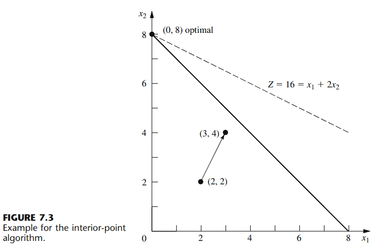
The algorithm begins with an initial trial solution that (like all subsequent trial solutions) lies in the interior of the feasible region, i.e., inside the boundary of the feasible region. Thus, for the example, the solution must not lie on any of the three lines $\left(x_1=0, x_2=0\right.$, $x_1+x_2=8$ ) that form the boundary of this region in Fig. 7.3. (A trial solution that lies on the boundary cannot be used because this would lead to the undefined mathematical operation of division by zero at one point in the algorithm.) We have arbitrarily chosen $\left(x_1, x_2\right)=(2,2)$ to be the initial trial solution.
To begin implementing concepts 1 and 2, note in Fig. 7.3 that the direction of movement from $(2,2)$ that increases $Z$ at the fastest possible rate is perpendicular to (and toward) the objective function line $Z=16=x_1+2 x_2$. We have shown this direction by the arrow from $(2,2)$ to $(3,4)$. Using vector addition, we have
$$
(3,4)=(2,2)+(1,2),
$$
where the vector $(1,2)$ is the gradient of the objective function. (We will discuss gradients further in Sec. 13.5 in the broader context of nonlinear programming, where algorithms similar to Karmarkar’s have long been used.) The components of $(1,2)$ are just the coefficients in the objective function. Thus, with one subsequent modification, the gradient $(1,2)$ defines the ideal direction to which to move, where the question of the distance to move will be considered later.
The algorithm actually operates on linear programming problems after they have been rewritten in augmented form. Letting $x_3$ be the slack variable for the functional constraint of the example, we see that this form is
$$
\text { Maximize } Z=x_1+2 x_2 \text {, }
$$
subject to
$$
x_1+x_2+x_3=8
$$
and
$$
x_1 \geq 0, \quad x_2 \geq 0, \quad x_3 \geq 0 .
$$
In matrix notation (slightly different from Chap. 5 because the slack variable now is incorporated into the notation), the augmented form can be written in general as
$$
\begin{aligned}
& \text { Maximize } Z=\mathbf{c}^T \mathbf{x}, \
& \text { subject to } \
& \mathbf{A x}=\mathbf{b}
\end{aligned}
$$
and
$$
\mathbf{x} \geq \mathbf{0},
$$
where
$$
\mathbf{c}=\left[\begin{array}{l}
1 \
2 \
0
\end{array}\right], \quad \mathbf{x}=\left[\begin{array}{l}
x_1 \
x_2 \
x_3
\end{array}\right], \quad \mathbf{A}=\left[\begin{array}{lll}
1, & 1, & 1
\end{array}\right], \quad \mathbf{b}=[8], \quad \mathbf{0}=\left[\begin{array}{l}
0 \
0 \
0
\end{array}\right]
$$
for the example. Note that $\mathbf{c}^T=[1,2,0]$ now is the gradient of the objective function.
数学代写|运筹学作业代写operational research代考|Using the Projected Gradient to Implement Concepts 1 and 2
In augmented form, the initial trial solution for the example is $\left(x_1, x_2, x_3\right)=(2,2,4)$. Adding the gradient $(1,2,0)$ leads to
$$
(3,4,4)=(2,2,4)+(1,2,0)
$$
However, now there is a complication. The algorithm cannot move from $(2,2,4)$ toward $(3,4,4)$, because $(3,4,4)$ is infeasible! When $x_1=3$ and $x_2=4$, then $x_3=8-x_1-$ $x_2=1$ instead of 4 . The point $(3,4,4)$ lies on the near side as you look down on the feasible triangle in Fig. 7.4. Therefore, to remain feasible, the algorithm (indirectly) projects the point $(3,4,4)$ down onto the feasible triangle by dropping a line that is perpendicular to this triangle. A vector from $(0,0,0)$ to $(1,1,1)$ is perpendicular to this triangle, so the perpendicular line through $(3,4,4)$ is given by the equation
$$
\left(x_1, x_2, x_3\right)=(3,4,4)-\theta(1,1,1) \text {, }
$$
where $\theta$ is a scalar. Since the triangle satisfies the equation $x_1+x_2+x_3=8$, this perpendicular line intersects the triangle at $(2,3,3)$. Because
$$
(2,3,3)=(2,2,4)+(0,1,-1),
$$
the projected gradient of the objective function (the gradient projected onto the feasible region) is $(0,1,-1)$. It is this projected gradient that defines the direction of movement for the algorithm, as shown by the arrow in Fig. 7.4.
A formula is available for computing the projected gradient directly. By defining the projection matrix $\mathbf{P}$ as
$$
\mathbf{P}=\mathbf{I}-\mathbf{A}^T\left(\mathbf{A} \mathbf{A}^T\right)^{-1} \mathbf{A},
$$
the projected gradient (in column form) is
$$
\mathbf{c}_p=\mathbf{P c} .
$$

运筹学代考
数学代写|运筹学作业代写operational research代考|The Relevance of the Gradient for Concepts 1 and 2
该算法从一个初始试解开始,该初始试解(像所有后续的试解一样)位于可行域的内部,即在可行域的边界内。因此,例如,解不得位于图7.3中形成该区域边界的三条线$\left(x_1=0, x_2=0\right.$, $x_1+x_2=8$中的任何一条线上。(不能使用位于边界上的试解,因为这将导致算法中某一点被零除的未定义数学操作。)我们任意选择$\left(x_1, x_2\right)=(2,2)$作为初始试解。
为了开始实现概念1和2,请注意图7.3中从$(2,2)$开始以最快的速度增加$Z$的运动方向垂直于(并朝向)目标函数线$Z=16=x_1+2 x_2$。我们用从$(2,2)$到$(3,4)$的箭头表示了这个方向。用向量加法,我们有
$$
(3,4)=(2,2)+(1,2),
$$
其中向量$(1,2)$是目标函数的梯度。(我们将在13.5节中在更广泛的非线性规划背景下进一步讨论梯度,在非线性规划中,类似Karmarkar的算法早已被使用。)$(1,2)$的分量就是目标函数的系数。因此,通过一个后续修改,梯度$(1,2)$定义了移动的理想方向,其中移动距离的问题将在稍后考虑。
该算法实际上是在线性规划问题被改写成增广形式后运行的。设$x_3$为本例函数约束的松弛变量,我们看到这种形式是
$$
\text { Maximize } Z=x_1+2 x_2 \text {, }
$$
以
$$
x_1+x_2+x_3=8
$$
和
$$
x_1 \geq 0, \quad x_2 \geq 0, \quad x_3 \geq 0 .
$$
在矩阵表示法中(与第5章略有不同,因为松弛变量现在被合并到表示法中),增广形式通常可以写成
$$
\begin{aligned}
& \text { Maximize } Z=\mathbf{c}^T \mathbf{x}, \
& \text { subject to } \
& \mathbf{A x}=\mathbf{b}
\end{aligned}
$$
和
$$
\mathbf{x} \geq \mathbf{0},
$$
在哪里
$$
\mathbf{c}=\left[\begin{array}{l}
1 \
2 \
0
\end{array}\right], \quad \mathbf{x}=\left[\begin{array}{l}
x_1 \
x_2 \
x_3
\end{array}\right], \quad \mathbf{A}=\left[\begin{array}{lll}
1, & 1, & 1
\end{array}\right], \quad \mathbf{b}=[8], \quad \mathbf{0}=\left[\begin{array}{l}
0 \
0 \
0
\end{array}\right]
$$
举个例子。注意$\mathbf{c}^T=[1,2,0]$现在是目标函数的梯度。
数学代写|运筹学作业代写operational research代考|Using the Projected Gradient to Implement Concepts 1 and 2
在增广形式中,该示例的初始试验解为$\left(x_1, x_2, x_3\right)=(2,2,4)$。添加渐变$(1,2,0)$导致
$$
(3,4,4)=(2,2,4)+(1,2,0)
$$
然而,现在有一个复杂的问题。算法不能从$(2,2,4)$移动到$(3,4,4)$,因为$(3,4,4)$是不可行的!当$x_1=3$和$x_2=4$时,则$x_3=8-x_1-$$x_2=1$而不是4。当你向下看图7.4中的可行三角形时,点$(3,4,4)$位于近侧。因此,为了保持可行,该算法(间接地)将点$(3,4,4)$投影到可行三角形上,方法是将一条垂直于可行三角形的直线向下投影。一个从$(0,0,0)$到$(1,1,1)$的向量垂直于这个三角形,所以通过$(3,4,4)$的垂直线由这个方程给出
$$
\left(x_1, x_2, x_3\right)=(3,4,4)-\theta(1,1,1) \text {, }
$$
其中$\theta$是标量。因为三角形满足方程$x_1+x_2+x_3=8$,所以这条垂线与三角形相交于$(2,3,3)$。因为
$$
(2,3,3)=(2,2,4)+(0,1,-1),
$$
目标函数的投影梯度(投影到可行区域上的梯度)为$(0,1,-1)$。正是这个投影梯度定义了算法的移动方向,如图7.4中的箭头所示。
给出了直接计算投影梯度的公式。通过定义投影矩阵$\mathbf{P}$为
$$
\mathbf{P}=\mathbf{I}-\mathbf{A}^T\left(\mathbf{A} \mathbf{A}^T\right)^{-1} \mathbf{A},
$$
投影梯度(以列形式)为
$$
\mathbf{c}_p=\mathbf{P c} .
$$

统计代写请认准statistics-lab™. statistics-lab™为您的留学生涯保驾护航。
金融工程代写
金融工程是使用数学技术来解决金融问题。金融工程使用计算机科学、统计学、经济学和应用数学领域的工具和知识来解决当前的金融问题,以及设计新的和创新的金融产品。
非参数统计代写
非参数统计指的是一种统计方法,其中不假设数据来自于由少数参数决定的规定模型;这种模型的例子包括正态分布模型和线性回归模型。
广义线性模型代考
广义线性模型(GLM)归属统计学领域,是一种应用灵活的线性回归模型。该模型允许因变量的偏差分布有除了正态分布之外的其它分布。
术语 广义线性模型(GLM)通常是指给定连续和/或分类预测因素的连续响应变量的常规线性回归模型。它包括多元线性回归,以及方差分析和方差分析(仅含固定效应)。
有限元方法代写
有限元方法(FEM)是一种流行的方法,用于数值解决工程和数学建模中出现的微分方程。典型的问题领域包括结构分析、传热、流体流动、质量运输和电磁势等传统领域。
有限元是一种通用的数值方法,用于解决两个或三个空间变量的偏微分方程(即一些边界值问题)。为了解决一个问题,有限元将一个大系统细分为更小、更简单的部分,称为有限元。这是通过在空间维度上的特定空间离散化来实现的,它是通过构建对象的网格来实现的:用于求解的数值域,它有有限数量的点。边界值问题的有限元方法表述最终导致一个代数方程组。该方法在域上对未知函数进行逼近。[1] 然后将模拟这些有限元的简单方程组合成一个更大的方程系统,以模拟整个问题。然后,有限元通过变化微积分使相关的误差函数最小化来逼近一个解决方案。
tatistics-lab作为专业的留学生服务机构,多年来已为美国、英国、加拿大、澳洲等留学热门地的学生提供专业的学术服务,包括但不限于Essay代写,Assignment代写,Dissertation代写,Report代写,小组作业代写,Proposal代写,Paper代写,Presentation代写,计算机作业代写,论文修改和润色,网课代做,exam代考等等。写作范围涵盖高中,本科,研究生等海外留学全阶段,辐射金融,经济学,会计学,审计学,管理学等全球99%专业科目。写作团队既有专业英语母语作者,也有海外名校硕博留学生,每位写作老师都拥有过硬的语言能力,专业的学科背景和学术写作经验。我们承诺100%原创,100%专业,100%准时,100%满意。
随机分析代写
随机微积分是数学的一个分支,对随机过程进行操作。它允许为随机过程的积分定义一个关于随机过程的一致的积分理论。这个领域是由日本数学家伊藤清在第二次世界大战期间创建并开始的。
时间序列分析代写
随机过程,是依赖于参数的一组随机变量的全体,参数通常是时间。 随机变量是随机现象的数量表现,其时间序列是一组按照时间发生先后顺序进行排列的数据点序列。通常一组时间序列的时间间隔为一恒定值(如1秒,5分钟,12小时,7天,1年),因此时间序列可以作为离散时间数据进行分析处理。研究时间序列数据的意义在于现实中,往往需要研究某个事物其随时间发展变化的规律。这就需要通过研究该事物过去发展的历史记录,以得到其自身发展的规律。
回归分析代写
多元回归分析渐进(Multiple Regression Analysis Asymptotics)属于计量经济学领域,主要是一种数学上的统计分析方法,可以分析复杂情况下各影响因素的数学关系,在自然科学、社会和经济学等多个领域内应用广泛。
MATLAB代写
MATLAB 是一种用于技术计算的高性能语言。它将计算、可视化和编程集成在一个易于使用的环境中,其中问题和解决方案以熟悉的数学符号表示。典型用途包括:数学和计算算法开发建模、仿真和原型制作数据分析、探索和可视化科学和工程图形应用程序开发,包括图形用户界面构建MATLAB 是一个交互式系统,其基本数据元素是一个不需要维度的数组。这使您可以解决许多技术计算问题,尤其是那些具有矩阵和向量公式的问题,而只需用 C 或 Fortran 等标量非交互式语言编写程序所需的时间的一小部分。MATLAB 名称代表矩阵实验室。MATLAB 最初的编写目的是提供对由 LINPACK 和 EISPACK 项目开发的矩阵软件的轻松访问,这两个项目共同代表了矩阵计算软件的最新技术。MATLAB 经过多年的发展,得到了许多用户的投入。在大学环境中,它是数学、工程和科学入门和高级课程的标准教学工具。在工业领域,MATLAB 是高效研究、开发和分析的首选工具。MATLAB 具有一系列称为工具箱的特定于应用程序的解决方案。对于大多数 MATLAB 用户来说非常重要,工具箱允许您学习和应用专业技术。工具箱是 MATLAB 函数(M 文件)的综合集合,可扩展 MATLAB 环境以解决特定类别的问题。可用工具箱的领域包括信号处理、控制系统、神经网络、模糊逻辑、小波、仿真等。