分类: AP统计代写

统计代写|AP统计代写AP统计代考|MAZ611U

如果你也在 怎样代写AP统计这个学科遇到相关的难题,请随时右上角联系我们的24/7代写客服。

 AP统计学与大学的统计学课程在核心内容上是一致的,只是涉及的深度稍浅,AP统计学主要包含以下四部分内容。 第一部分 如何获取数据,获取数据的方式有哪些呢? 获取数据的方式主要包括普查、抽样调查、观测研究和实验设计等。

statistics-lab™ 为您的留学生涯保驾护航 在代写AP统计方面已经树立了自己的口碑, 保证靠谱, 高质且原创的统计Statistics代写服务。我们的专家在代写AP统计代写方面经验极为丰富,各种代写AP统计相关的作业也就用不着说。

我们提供的AP统计及其相关学科的代写,服务范围广, 其中包括但不限于:

  • Statistical Inference 统计推断
  • Statistical Computing 统计计算
  • Advanced Probability Theory 高等概率论
  • Advanced Mathematical Statistics 高等数理统计学
  • (Generalized) Linear Models 广义线性模型
  • Statistical Machine Learning 统计机器学习
  • Longitudinal Data Analysis 纵向数据分析
  • Foundations of Data Science 数据科学基础
统计代写|AP统计代写AP统计代考|MAZ611U

统计代写|AP统计代写AP统计代考|General Test-Taking Tips

Much of being good at test-taking is experience. Your own test-taking history and these tips should help you demonstrate what you know (and you know a lot) on the exam. The tips in this section are of a general nature-they apply to taking tests in general as well as to both multiple-choice and free-response type questions.

  1. Look over the entire exam first, whichever part you are working on. With the exception of, maybe, Question #1 in each section, the questions are not presented in order of difficulty. Find and do the easy questions first.
  2. Don’t spend too much time on any one question. Remember that you have an average of slightly more than two minutes for each multiple-choice question, $12-13$ minutes for Questions 1-5 of the free-response section, and 25-30 minutes for the investigative task. Some questions are very short and will give you extra time to spend on the more difficult questions. At the other time extreme, spending 10 minutes on one multiplechoice question (or 30 minutes on one free-response question) is not a good use of time-you won’t have time to finish.
  3. Become familiar with the instructions for the different parts of the exam before the day of the exam. You don’t want to have to waste time figuring out how to process the exam. You’ll have your hands full using the available time figuring out how to do the questions. Look at the Practice Exams at the end of this book so you understand the nature of the test.
  4. Be neat! On the Statistics exam, communication is very important. This means no smudges on the multiple-choice part of the exam and legible responses on the free-response. A machine may score a smudge as incorrect and readers will spend only so long trying to decipher your handwriting.
  5. Practice working as many exam-like problems as you can in the weeks before the exam. This will help you know which statistical technique to choose on each question. It’s a great feeling to see a problem on the exam and know that you can do it quickly and easily because it’s just like a problem you’ve practiced on.
  6. Make sure your calculator has new batteries. There’s nothing worse than a “Replace batteries now” warning at the start of the exam. Bring a spare calculator if you have or can borrow one (you are allowed to have two calculators).
  7. Bring a supply of sharpened pencils to the exam. You don’t want to have to waste time walking to the pencil sharpener during the exam. (The other students will be grateful for the quiet, as well.) Also, bring a good-quality eraser to the exam so that any erasures are neat and complete.
  8. Get a good night’s sleep before the exam. You’ll do your best if you are relaxed and confident in your knowledge. If you don’t know the material by the night before the exam, you aren’t going to learn it in one evening. Relax. Maybe watch an early movie. If you know your stuff and aren’t overly tired, you should do fine.

统计代写|AP统计代写AP统计代考|Tips for Multiple-Choice Questions

There are whole industries dedicated to teaching you how to take a test. In reality, no amount of test-taking strategy will replace knowledge of the subject. If you are on top of the subject, you’ll most likely do well even if you haven’t paid $\$ 500$ for a test-prep course.

The following tips, when combined with your statistics knowledge, should help you do well.

  1. Read the question carefully before beginning. A lot of mistakes get made because students don’t completely understand the question before trying to answer it. The result is that they will often answer a different question than they were asked.
  2. Try to answer the question before you look at the answers. Looking at the choices and trying to figure out which one works best is not a good strategy. You run the risk of being led astray by an incorrect answer. Instead, try to answer the question first, as if there was just a blank for the answer and no choices.
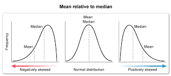
  3. Understand that the incorrect answers (which are called distractors) are designed to appear reasonable. Watch out for words like never and always in answer choices. These frequently indicate distractors. Don’t get suckered into choosing an answer just because it sounds good! The question designers try to make all the logical mistakes you might make and the answers they come up with become the distractors. For example, suppose you are asked for the median of the five numbers $3,4,6,7$, and 15 . The correct answer is 6 (the middle score in the ordered list). But suppose you misread the question and calculated the mean instead. You’d get 7 and, be assured, 7 will appear as one of the distractors.
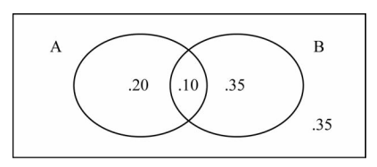
  4. Drawing a picture can often help visualize the situation described in the problem. Sometimes, relationships become clearer when a picture is used to display them. For example, using Venn diagrams can often help you “see” the nature of a probability problem. Another example would be using a graph or a scatterplot of some given data as part of doing a regression analysis.
  5. Answer each question. You will earn one point for each correct answer. Incorrect answers are worth zero points and no points are earned for blank responses. If you aren’t sure of an answer, eliminate as many choices as you can, then guess.
  6. Double check that you have (a) answered the question you are working on, especially if you’ve left some questions blank (it’s horrible to realize at some point that all of your responses are one question off!) and (b) that you have filled in the correct bubble for your answer. If you need to make changes, make sure you erase completely and neatly.
统计代写|AP统计代写AP统计代考|MAZ611U

AP统计代写

统计代写|AP统计代写AP统计代考|General Test-Taking Tips

擅长应试的很大一部分是经验。您自己的考试历史和这些提示应该可以帮助您展示您在考试中所知道的(并且您知道的很多)。本节中的提示具有一般性质——它们适用于一般考试以及多项选择题和自由回答题。

  1. 首先查看整个考试,无论您正在研究哪个部分。除了每个部分中的问题 #1 之外,这些问题没有按难度顺序排列。首先找到并做简单的问题。
  2. 不要在任何一个问题上花费太多时间。请记住,每个多项选择题的平均时间略多于两分钟,12−13自由回答部分的问题 1-5 分钟,调查任务 25-30 分钟。有些问题很短,会给你额外的时间来解决更难的问题。在另一个极端情况下,在一个多项选择题上花费 10 分钟(或在一个自由回答问题上花费 30 分钟)并不是一种很好的时间利用方式——你将没有时间完成。
  3. 在考试前熟悉考试不同部分的说明。您不想浪费时间弄清楚如何处理考试。您将充分利用可用的时间来弄清楚如何做这些问题。查看本书末尾的练习考试,以便了解考试的性质。
  4. 保持整洁!在统计学考试中,沟通非常重要。这意味着考试的多项选择部分没有污点,自由回答的答案清晰易读。机器可能会将污迹记为不正确,而读者只会花很长时间尝试破译您的笔迹。
  5. 在考试前的几周内尽可能多地练习解决类似考试的问题。这将帮助您了解在每个问题上选择哪种统计技术。在考试中看到一个问题并知道您可以快速轻松地完成它是一种很棒的感觉,因为它就像您练习过的问题一样。
  6. 确保您的计算器有新电池。没有什么比考试开始时出现“立即更换电池”警告更糟糕的了。如果您有或可以借用一个备用计算器(您可以拥有两个计算器)。
  7. 考试时带上削尖的铅笔。您不想在考试期间浪费时间走到卷笔刀旁。(其他学生也会因为安静而感激。)另外,考试时带上质量好的橡皮擦,这样任何擦除都整齐完整。
  8. 考试前睡个好觉。如果您对自己的知识感到放松和自信,您会尽力而为。如果你在考试前一晚还不知道这些材料,你就不会在一个晚上学会它。放松。也许看一部早期的电影。如果您知道自己的东西并且不太累,那么您应该做得很好。

统计代写|AP统计代写AP统计代考|Tips for Multiple-Choice Questions

整个行业都致力于教你如何参加考试。实际上,再多的应试策略也无法取代对这门学科的了解。如果你掌握了这个主题,即使你没有付钱,你也很可能会做得很好$500备考课程。

以下提示与您的统计知识相结合,应该可以帮助您做得更好。

  1. 在开始之前仔细阅读问题。因为学生在尝试回答之前没有完全理解问题,所以会犯很多错误。结果是他们经常会回答与他们被问到的不同的问题。
  2. 在查看答案之前尝试回答问题。查看选择并试图找出哪个最有效并不是一个好策略。你冒着被错误答案误导的风险。相反,试着先回答这个问题,好像答案只有一个空白,没有选择。
  3. 理解不正确的答案(称为干扰项)是为了显得合理而设计的。在答案选择中注意像从不和总是这样的词。这些经常表明干扰因素。不要仅仅因为听起来不错就选择一个答案!问题设计者试图犯下你可能犯的所有逻辑错误,而他们提出的答案会分散注意力。例如,假设您被要求输入五个数字的中位数3,4,6,7, 和 15 . 正确答案是 6(排序列表中的中间分数)。但是假设您误读了问题并计算了平均值。你会得到 7,而且,请放心,7 将作为干扰因素之一出现。
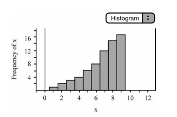
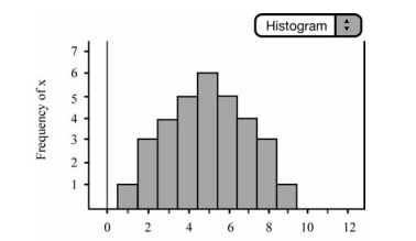
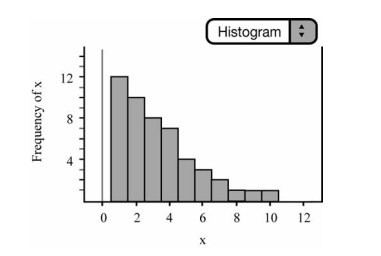
  4. 绘制图片通常可以帮助形象化问题中描述的情况。有时,当使用图片显示它们时,关系会变得更加清晰。例如,使用维恩图通常可以帮助您“了解”概率问题的本质。另一个例子是使用一些给定数据的图表或散点图作为回归分析的一部分。
  5. 回答每个问题。每答对一题,您将获得一分。不正确的答案是零分,空白回答不得分。如果您不确定答案,请消除尽可能多的选择,然后猜测。
  6. 仔细检查您是否 (a) 回答了您正在处理的问题,特别是如果您将一些问题留空(在某些时候意识到您的所有回答都是一个问题,这太可怕了!)和 (b) 您已为您的答案填入正确的气泡。如果您需要进行更改,请确保您完全整齐地擦除。
统计代写|AP统计代写AP统计代考 请认准statistics-lab™

统计代写请认准statistics-lab™. statistics-lab™为您的留学生涯保驾护航。

金融工程代写

金融工程是使用数学技术来解决金融问题。金融工程使用计算机科学、统计学、经济学和应用数学领域的工具和知识来解决当前的金融问题,以及设计新的和创新的金融产品。

非参数统计代写

非参数统计指的是一种统计方法,其中不假设数据来自于由少数参数决定的规定模型;这种模型的例子包括正态分布模型和线性回归模型。

广义线性模型代考

广义线性模型(GLM)归属统计学领域,是一种应用灵活的线性回归模型。该模型允许因变量的偏差分布有除了正态分布之外的其它分布。

术语 广义线性模型(GLM)通常是指给定连续和/或分类预测因素的连续响应变量的常规线性回归模型。它包括多元线性回归,以及方差分析和方差分析(仅含固定效应)。

有限元方法代写

有限元方法(FEM)是一种流行的方法,用于数值解决工程和数学建模中出现的微分方程。典型的问题领域包括结构分析、传热、流体流动、质量运输和电磁势等传统领域。

有限元是一种通用的数值方法,用于解决两个或三个空间变量的偏微分方程(即一些边界值问题)。为了解决一个问题,有限元将一个大系统细分为更小、更简单的部分,称为有限元。这是通过在空间维度上的特定空间离散化来实现的,它是通过构建对象的网格来实现的:用于求解的数值域,它有有限数量的点。边界值问题的有限元方法表述最终导致一个代数方程组。该方法在域上对未知函数进行逼近。[1] 然后将模拟这些有限元的简单方程组合成一个更大的方程系统,以模拟整个问题。然后,有限元通过变化微积分使相关的误差函数最小化来逼近一个解决方案。

tatistics-lab作为专业的留学生服务机构,多年来已为美国、英国、加拿大、澳洲等留学热门地的学生提供专业的学术服务,包括但不限于Essay代写,Assignment代写,Dissertation代写,Report代写,小组作业代写,Proposal代写,Paper代写,Presentation代写,计算机作业代写,论文修改和润色,网课代做,exam代考等等。写作范围涵盖高中,本科,研究生等海外留学全阶段,辐射金融,经济学,会计学,审计学,管理学等全球99%专业科目。写作团队既有专业英语母语作者,也有海外名校硕博留学生,每位写作老师都拥有过硬的语言能力,专业的学科背景和学术写作经验。我们承诺100%原创,100%专业,100%准时,100%满意。

随机分析代写


随机微积分是数学的一个分支,对随机过程进行操作。它允许为随机过程的积分定义一个关于随机过程的一致的积分理论。这个领域是由日本数学家伊藤清在第二次世界大战期间创建并开始的。

时间序列分析代写

随机过程,是依赖于参数的一组随机变量的全体,参数通常是时间。 随机变量是随机现象的数量表现,其时间序列是一组按照时间发生先后顺序进行排列的数据点序列。通常一组时间序列的时间间隔为一恒定值(如1秒,5分钟,12小时,7天,1年),因此时间序列可以作为离散时间数据进行分析处理。研究时间序列数据的意义在于现实中,往往需要研究某个事物其随时间发展变化的规律。这就需要通过研究该事物过去发展的历史记录,以得到其自身发展的规律。

回归分析代写

多元回归分析渐进(Multiple Regression Analysis Asymptotics)属于计量经济学领域,主要是一种数学上的统计分析方法,可以分析复杂情况下各影响因素的数学关系,在自然科学、社会和经济学等多个领域内应用广泛。

MATLAB代写

MATLAB 是一种用于技术计算的高性能语言。它将计算、可视化和编程集成在一个易于使用的环境中,其中问题和解决方案以熟悉的数学符号表示。典型用途包括:数学和计算算法开发建模、仿真和原型制作数据分析、探索和可视化科学和工程图形应用程序开发,包括图形用户界面构建MATLAB 是一个交互式系统,其基本数据元素是一个不需要维度的数组。这使您可以解决许多技术计算问题,尤其是那些具有矩阵和向量公式的问题,而只需用 C 或 Fortran 等标量非交互式语言编写程序所需的时间的一小部分。MATLAB 名称代表矩阵实验室。MATLAB 最初的编写目的是提供对由 LINPACK 和 EISPACK 项目开发的矩阵软件的轻松访问,这两个项目共同代表了矩阵计算软件的最新技术。MATLAB 经过多年的发展,得到了许多用户的投入。在大学环境中,它是数学、工程和科学入门和高级课程的标准教学工具。在工业领域,MATLAB 是高效研究、开发和分析的首选工具。MATLAB 具有一系列称为工具箱的特定于应用程序的解决方案。对于大多数 MATLAB 用户来说非常重要,工具箱允许您学习应用专业技术。工具箱是 MATLAB 函数(M 文件)的综合集合,可扩展 MATLAB 环境以解决特定类别的问题。可用工具箱的领域包括信号处理、控制系统、神经网络、模糊逻辑、小波、仿真等。

R语言代写问卷设计与分析代写
PYTHON代写回归分析与线性模型代写
MATLAB代写方差分析与试验设计代写
STATA代写机器学习/统计学习代写
SPSS代写计量经济学代写
EVIEWS代写时间序列分析代写
EXCEL代写深度学习代写
SQL代写各种数据建模与可视化代写

英国补考|AP统计代写AP统计代考|MT605B

如果你也在 怎样代写AP统计这个学科遇到相关的难题,请随时右上角联系我们的24/7代写客服。

 AP统计学与大学的统计学课程在核心内容上是一致的,只是涉及的深度稍浅,AP统计学主要包含以下四部分内容。 第一部分 如何获取数据,获取数据的方式有哪些呢? 获取数据的方式主要包括普查、抽样调查、观测研究和实验设计等。

statistics-lab™ 为您的留学生涯保驾护航 在代写AP统计方面已经树立了自己的口碑, 保证靠谱, 高质且原创的统计Statistics代写服务。我们的专家在代写AP统计代写方面经验极为丰富,各种代写AP统计相关的作业也就用不着说。

我们提供的AP统计及其相关学科的代写,服务范围广, 其中包括但不限于:

  • Statistical Inference 统计推断
  • Statistical Computing 统计计算
  • Advanced Probability Theory 高等概率论
  • Advanced Mathematical Statistics 高等数理统计学
  • (Generalized) Linear Models 广义线性模型
  • Statistical Machine Learning 统计机器学习
  • Longitudinal Data Analysis 纵向数据分析
  • Foundations of Data Science 数据科学基础
英国补考|AP统计代写AP统计代考|MT605B

英国补考|AP统计代写AP统计代考|Three Approaches to Preparing for the AP Statistics Exam

No one knows your study habits, likes, and dislikes better than you. So, you are the only one who can decide which approach you want and/or need, to adopt to prepare for the AP Statistics exam. This may help you place yourself in a particular prep mode. This chapter presents three possible study plans, labeled A, B, and C. Look at the brief profiles below and try to determine which of these three plans is right for you.
You’re a full-school-year prep student if:

  1. You are the kind of person who likes to plan for everything far in advance.
  2. You arrive at the airport two hours before your flight.
  3. You like detailed planning and everything in its place.
  4. You feel that you must be thoroughly prepared.
  5. You hate surprises.
    If you fit this profile, consider Plan A.

You’re a one-semester prep student if:

  1. You get to the airport one hour before your flight is scheduled to leave.
  2. You are willing to plan ahead to feel comfortable in stressful situations, but are okay with skipping some details.
  3. You feel more comfortable when you know what to expect, but a surprise or two is $\mathrm{OK}$.
  4. You are always on time for appointments.
    If you fit this profile, consider Plan $\mathbf{B}$.
    You’re a 6-week prep student if:
  5. You get to the airport at the last possible moment.
  6. You work best under pressure and tight deadlines.
  7. You feel very confident with the skills and background you’ve learned in your AP Statistics class.
  8. You decided late in the year to take the exam.
  9. You like surprises.
  10. You feel okay if you arrive 10-15 minutes late for an appointment.
    If you fit this profile, consider Plan $\mathbf{C}$.

英国补考|AP统计代写AP统计代考|SOLUTIONS TO DIAGNOSTIC TEST—SECTION

We would expect the residual for $5.5$ to be in the same general area as the residuals for $4,5,6$, and 7 (circled on the graph). The residuals in this area are all positive $\Rightarrow$ actual $-$ predicted $>0 \Rightarrow$ actual $>$ predicted. The prediction would probably be too small.

  1. a. It is an observational study. The researcher made no attempt to impose a treatment on the subjects in the study. The hired person simply observed and recorded behavior.
    b. – The article made no mention of the sample size. Without that you are unable to judge how much sampling variability there might have been. It’s possible that the 63-59 split was attributable to sampling variability.
  • The study was done at one Scorebucks, on one morning, for a single 2-hour period. The population at that Scorebucks might differ in some significant way from the patrons at other Scorebucks around the city (and there are many, many of them). It might have been different on a different day or during a different time of the day. A single 2-hour period may not have been enough time to collect sufficient data (we don’t know because the sample size wasn’t given) and, again, a 2-hour period in the afternoon might have yielded different results.
    c. You would conduct the study at multiple Scorebucks, possibly blocking by location if you believe that might make a difference (i.e., would a working-class neighborhood have different preferences than the ritziest neighborhood?). You would observe at different times of the day and on different days. You would make sure that the total sample size was large enough to control for sampling variability (replication).
英国补考|AP统计代写AP统计代考|MT605B

AP统计代写

英国补考|AP统计代写AP统计代考|Three Approaches to Preparing for the AP Statistics Exam

没有人比你更了解你的学习习惯、好恶。因此,您是唯一可以决定您想要和/或需要采用哪种方法来准备 AP 统计考试的人。这可以帮助您将自己置于特定的准备模式。本章介绍了三种可能的学习计划,分别标记为 A、B 和 C。请查看下面的简要介绍,并尝试确定这三个计划中的哪一个适合您。
如果满足以下条件,您是全学年预科学生:

  1. 你是那种喜欢提前计划好一切的人。
  2. 您在航班起飞前两小时到达机场。
  3. 你喜欢详细的计划和一切。
  4. 你觉得你必须做好充分的准备。
  5. 你讨厌惊喜。
    如果您符合此配置文件,请考虑计划 A。

如果满足以下条件,您是一个学期的预科生:

  1. 您在航班计划起飞前一小时到达机场。
  2. 您愿意提前计划以在压力大的情况下感到舒适,但可以跳过一些细节。
  3. 当您知道会发生什么时,您会感觉更舒服,但是一两个惊喜是○ķ.
  4. 您总是准时赴约。
    如果您符合此配置文件,请考虑计划乙.
    如果满足以下条件,您是为期 6 周的预科学生:
  5. 你会在最后一刻到达机场。
  6. 你在压力和紧迫的期限内工作得最好。
  7. 你对你在 AP 统计课上学到的技能和背景感到非常自信。
  8. 你决定在年底参加考试。
  9. 你喜欢惊喜。
  10. 如果约会迟到 10 到 15 分钟,您会感觉很好。
    如果您符合此配置文件,请考虑计划C.

英国补考|AP统计代写AP统计代考|SOLUTIONS TO DIAGNOSTIC TEST—SECTION

我们预计残差为5.5与残差在同一区域内4,5,6, 和 7(在图表上圈出)。该区域的残差都是正数⇒实际的−预料到的>0⇒实际的>预料到的。预测可能太小了。

  1. 一个。这是一项观察性研究。研究人员没有试图对研究中的受试者施加治疗。被雇用的人只是观察和记录行为。
    湾。– 文章没有提到样本量。否则,您将无法判断可能存在多少抽样可变性。63-59 的分裂可能是由于抽样的变异性。
  • 这项研究是在一天早上用一个 Scorebucks 完成的,时间为 2 小时。该 Scorebucks 的人口可能与城市周围其他 Scorebucks 的顾客有一些显着差异(而且有很多很多)。在不同的一天或一天​​中的不同时间可能会有所不同。单个 2 小时的时间可能不足以收集足够的数据(我们不知道,因为没有给出样本量),同样,下午的 2 小时可能会产生不同的结果。
    C。您将在多个 Scorebucks 进行研究,如果您认为这可能会产生影响,可能会按位置进行阻止(即,工人阶级社区的偏好会与最豪华的社区不同吗?)。你会在一天中的不同时间和不同的日子观察。您将确保总样本量足够大以控制抽样变异性(复制)。
统计代写|AP统计代写AP统计代考 请认准statistics-lab™

统计代写请认准statistics-lab™. statistics-lab™为您的留学生涯保驾护航。

金融工程代写

金融工程是使用数学技术来解决金融问题。金融工程使用计算机科学、统计学、经济学和应用数学领域的工具和知识来解决当前的金融问题,以及设计新的和创新的金融产品。

非参数统计代写

非参数统计指的是一种统计方法,其中不假设数据来自于由少数参数决定的规定模型;这种模型的例子包括正态分布模型和线性回归模型。

广义线性模型代考

广义线性模型(GLM)归属统计学领域,是一种应用灵活的线性回归模型。该模型允许因变量的偏差分布有除了正态分布之外的其它分布。

术语 广义线性模型(GLM)通常是指给定连续和/或分类预测因素的连续响应变量的常规线性回归模型。它包括多元线性回归,以及方差分析和方差分析(仅含固定效应)。

有限元方法代写

有限元方法(FEM)是一种流行的方法,用于数值解决工程和数学建模中出现的微分方程。典型的问题领域包括结构分析、传热、流体流动、质量运输和电磁势等传统领域。

有限元是一种通用的数值方法,用于解决两个或三个空间变量的偏微分方程(即一些边界值问题)。为了解决一个问题,有限元将一个大系统细分为更小、更简单的部分,称为有限元。这是通过在空间维度上的特定空间离散化来实现的,它是通过构建对象的网格来实现的:用于求解的数值域,它有有限数量的点。边界值问题的有限元方法表述最终导致一个代数方程组。该方法在域上对未知函数进行逼近。[1] 然后将模拟这些有限元的简单方程组合成一个更大的方程系统,以模拟整个问题。然后,有限元通过变化微积分使相关的误差函数最小化来逼近一个解决方案。

tatistics-lab作为专业的留学生服务机构,多年来已为美国、英国、加拿大、澳洲等留学热门地的学生提供专业的学术服务,包括但不限于Essay代写,Assignment代写,Dissertation代写,Report代写,小组作业代写,Proposal代写,Paper代写,Presentation代写,计算机作业代写,论文修改和润色,网课代做,exam代考等等。写作范围涵盖高中,本科,研究生等海外留学全阶段,辐射金融,经济学,会计学,审计学,管理学等全球99%专业科目。写作团队既有专业英语母语作者,也有海外名校硕博留学生,每位写作老师都拥有过硬的语言能力,专业的学科背景和学术写作经验。我们承诺100%原创,100%专业,100%准时,100%满意。

随机分析代写


随机微积分是数学的一个分支,对随机过程进行操作。它允许为随机过程的积分定义一个关于随机过程的一致的积分理论。这个领域是由日本数学家伊藤清在第二次世界大战期间创建并开始的。

时间序列分析代写

随机过程,是依赖于参数的一组随机变量的全体,参数通常是时间。 随机变量是随机现象的数量表现,其时间序列是一组按照时间发生先后顺序进行排列的数据点序列。通常一组时间序列的时间间隔为一恒定值(如1秒,5分钟,12小时,7天,1年),因此时间序列可以作为离散时间数据进行分析处理。研究时间序列数据的意义在于现实中,往往需要研究某个事物其随时间发展变化的规律。这就需要通过研究该事物过去发展的历史记录,以得到其自身发展的规律。

回归分析代写

多元回归分析渐进(Multiple Regression Analysis Asymptotics)属于计量经济学领域,主要是一种数学上的统计分析方法,可以分析复杂情况下各影响因素的数学关系,在自然科学、社会和经济学等多个领域内应用广泛。

MATLAB代写

MATLAB 是一种用于技术计算的高性能语言。它将计算、可视化和编程集成在一个易于使用的环境中,其中问题和解决方案以熟悉的数学符号表示。典型用途包括:数学和计算算法开发建模、仿真和原型制作数据分析、探索和可视化科学和工程图形应用程序开发,包括图形用户界面构建MATLAB 是一个交互式系统,其基本数据元素是一个不需要维度的数组。这使您可以解决许多技术计算问题,尤其是那些具有矩阵和向量公式的问题,而只需用 C 或 Fortran 等标量非交互式语言编写程序所需的时间的一小部分。MATLAB 名称代表矩阵实验室。MATLAB 最初的编写目的是提供对由 LINPACK 和 EISPACK 项目开发的矩阵软件的轻松访问,这两个项目共同代表了矩阵计算软件的最新技术。MATLAB 经过多年的发展,得到了许多用户的投入。在大学环境中,它是数学、工程和科学入门和高级课程的标准教学工具。在工业领域,MATLAB 是高效研究、开发和分析的首选工具。MATLAB 具有一系列称为工具箱的特定于应用程序的解决方案。对于大多数 MATLAB 用户来说非常重要,工具箱允许您学习应用专业技术。工具箱是 MATLAB 函数(M 文件)的综合集合,可扩展 MATLAB 环境以解决特定类别的问题。可用工具箱的领域包括信号处理、控制系统、神经网络、模糊逻辑、小波、仿真等。

R语言代写问卷设计与分析代写
PYTHON代写回归分析与线性模型代写
MATLAB代写方差分析与试验设计代写
STATA代写机器学习/统计学习代写
SPSS代写计量经济学代写
EVIEWS代写时间序列分析代写
EXCEL代写深度学习代写
SQL代写各种数据建模与可视化代写

统计代写|AP统计代写AP统计代考|MT605A

如果你也在 怎样代写AP统计这个学科遇到相关的难题,请随时右上角联系我们的24/7代写客服。

 AP统计学与大学的统计学课程在核心内容上是一致的,只是涉及的深度稍浅,AP统计学主要包含以下四部分内容。 第一部分 如何获取数据,获取数据的方式有哪些呢? 获取数据的方式主要包括普查、抽样调查、观测研究和实验设计等。

statistics-lab™ 为您的留学生涯保驾护航 在代写AP统计方面已经树立了自己的口碑, 保证靠谱, 高质且原创的统计Statistics代写服务。我们的专家在代写AP统计代写方面经验极为丰富,各种代写AP统计相关的作业也就用不着说。

我们提供的AP统计及其相关学科的代写,服务范围广, 其中包括但不限于:

  • Statistical Inference 统计推断
  • Statistical Computing 统计计算
  • Advanced Probability Theory 高等概率论
  • Advanced Mathematical Statistics 高等数理统计学
  • (Generalized) Linear Models 广义线性模型
  • Statistical Machine Learning 统计机器学习
  • Longitudinal Data Analysis 纵向数据分析
  • Foundations of Data Science 数据科学基础
统计代写|AP统计代写AP统计代考|MT605A

统计代写|AP统计代写AP统计代考|Who Writes the AP Statistics Exam

Development of each AP exam is a multiyear effort that involves many education and testing professionals and students. At the heart of the effort is the AP Statistics Test Development Committee, a group of college and high school statistics teachers who are typically asked to serve for three years. The committee and other college professors create a large pool of multiple-choice questions. With the help of the testing experts at Educational Testing Service (ETS), these questions are then pretested with college students enrolled in Statistics courses for accuracy, appropriateness, clarity, and assurance that there is only one possible answer. The results of this pretesting allow each question to be categorized by degree of difficulty.

The free-response essay questions that make up Section II go through a similar process of creation, modification, pretesting, and final refinement so that the questions cover the necessary areas of material and are at an appropriate level of difficulty and clarity. The committee also makes a great deal of effort to construct a free-response exam that will allow for clear and equitable grading by the AP readers.

At the conclusion of each AP reading and scoring of exams, the exam itself and the results are thoroughly evaluated by the committee and by ETS. In this way, the College Board can use the results to make suggestions for course development in high schools and to plan future exams.

统计代写|AP统计代写AP统计代考|What Is the Graphing Calculator Policy

The following is the policy on graphing calculators as stated on the College Board’s AP Central Web site:

Each student is expected to bring to the exam a graphing calculator with statistical capabilities. The computational capabilities should include standard statistical univariate and bivariate summaries, through linear regression. The graphical capabilities should include common univariate and bivariate displays such as histograms, boxplots, and scatterplots.

  • You can bring two calculators to the exam.
  • The calculator memory will not be cleared but you may only use the memory to store programs, not notes.
  • For the exam, you’re not allowed to access any information in your graphing calculators or elsewhere if it’s not directly related to upgrading the statistical functionality of older graphing calculators to make them comparable to statistical features found on newer models. The only acceptable upgrades are those that improve the computational functionalities and/or graphical functionalities for data you key into the calculator while taking the examination. Unacceptable enhancements include, but aren’t limited to, keying or scanning text or response templates into the calculator.

During the exam, you can’t use minicomputers, pocket organizers, electronic writing pads, or calculators with QWERTY (i.e., typewriter) keyboards.

You may use a calculator to do needed computations. However, remember that the person reading your exam needs to see your reasoning in order to score your exam. Your teacher can check for a list of acceptable calculators on AP Central. The TI-83/84 is certainly OK.

统计代写|AP统计代写AP统计代考|MT605A

AP统计代写

统计代写|AP统计代写AP统计代考|Who Writes the AP Statistics Exam

每个 AP 考试的开发都是一项多年的工作,涉及许多教育和测试专业人​​士和学生。这项工作的核心是 AP 统计测试发展委员会,这是一群大学和高中统计教师,他们通常被要求服务三年。委员会和其他大学教授创建了大量的多项选择题。在教育测试服务中心 (ETS) 的测试专家的帮助下,这些问题将由参加统计课程的大学生进行预测试,以确保其准确性、适当性、清晰性,并确保只有一个可能的答案。该预测试的结果允许按难度对每个问题进行分类。

构成第二部分的自由回答论文问题经历了类似的创建、修改、预测试和最终完善的过程,以便问题涵盖必要的材料领域,并具有适当的难度和清晰度。委员会还做出了巨大的努力来构建一个自由回答的考试,这将使 AP 读者能够清晰和公平地评分。

在每次 AP 阅读和考试评分结束时,委员会和 ETS 都会对考试本身和结果进行全面评估。这样,大学理事会就可以利用这些结果为高中的课程发展提出建议,并计划未来的考试。

统计代写|AP统计代写AP统计代考|What Is the Graphing Calculator Policy

以下是美国大学理事会 AP Central 网站上关于图形计算器的政策:

每个学生都应携带具有统计功能的图形计算器参加考试。计算能力应包括标准统计单变量和双变量汇总,通过线性回归。图形功能应包括常见的单变量和双变量显示,例如直方图、箱线图和散点图。

  • 您可以带两个计算器参加考试。
  • 计算器内存不会被清除,但您只能使用内存来存储程序,而不是笔记。
  • 对于考试,如果与升级旧图形计算器的统计功能没有直接关系,则不允许您访问图形计算器或其他地方的任何信息,以使其与新模型上的统计功能相媲美。唯一可接受的升级是那些改进了您在考试时输入计算器的数据的计算功能和/或图形功能。不可接受的增强包括但不限于将文本或响应模板键入或扫描到计算器中。

在考试期间,您不能使用带有 QWERTY(即打字机)键盘的小型计算机、袖珍管理器、电子书写板或计算器。

您可以使用计算器进行所需的计算。但是,请记住,阅读您的考试的人需要看到您的推理才能为您的考试评分。您的老师可以在 AP Central 上查看可接受的计算器列表。TI-83/84 肯定没问题。

统计代写|AP统计代写AP统计代考 请认准statistics-lab™

统计代写请认准statistics-lab™. statistics-lab™为您的留学生涯保驾护航。

金融工程代写

金融工程是使用数学技术来解决金融问题。金融工程使用计算机科学、统计学、经济学和应用数学领域的工具和知识来解决当前的金融问题,以及设计新的和创新的金融产品。

非参数统计代写

非参数统计指的是一种统计方法,其中不假设数据来自于由少数参数决定的规定模型;这种模型的例子包括正态分布模型和线性回归模型。

广义线性模型代考

广义线性模型(GLM)归属统计学领域,是一种应用灵活的线性回归模型。该模型允许因变量的偏差分布有除了正态分布之外的其它分布。

术语 广义线性模型(GLM)通常是指给定连续和/或分类预测因素的连续响应变量的常规线性回归模型。它包括多元线性回归,以及方差分析和方差分析(仅含固定效应)。

有限元方法代写

有限元方法(FEM)是一种流行的方法,用于数值解决工程和数学建模中出现的微分方程。典型的问题领域包括结构分析、传热、流体流动、质量运输和电磁势等传统领域。

有限元是一种通用的数值方法,用于解决两个或三个空间变量的偏微分方程(即一些边界值问题)。为了解决一个问题,有限元将一个大系统细分为更小、更简单的部分,称为有限元。这是通过在空间维度上的特定空间离散化来实现的,它是通过构建对象的网格来实现的:用于求解的数值域,它有有限数量的点。边界值问题的有限元方法表述最终导致一个代数方程组。该方法在域上对未知函数进行逼近。[1] 然后将模拟这些有限元的简单方程组合成一个更大的方程系统,以模拟整个问题。然后,有限元通过变化微积分使相关的误差函数最小化来逼近一个解决方案。

tatistics-lab作为专业的留学生服务机构,多年来已为美国、英国、加拿大、澳洲等留学热门地的学生提供专业的学术服务,包括但不限于Essay代写,Assignment代写,Dissertation代写,Report代写,小组作业代写,Proposal代写,Paper代写,Presentation代写,计算机作业代写,论文修改和润色,网课代做,exam代考等等。写作范围涵盖高中,本科,研究生等海外留学全阶段,辐射金融,经济学,会计学,审计学,管理学等全球99%专业科目。写作团队既有专业英语母语作者,也有海外名校硕博留学生,每位写作老师都拥有过硬的语言能力,专业的学科背景和学术写作经验。我们承诺100%原创,100%专业,100%准时,100%满意。

随机分析代写


随机微积分是数学的一个分支,对随机过程进行操作。它允许为随机过程的积分定义一个关于随机过程的一致的积分理论。这个领域是由日本数学家伊藤清在第二次世界大战期间创建并开始的。

时间序列分析代写

随机过程,是依赖于参数的一组随机变量的全体,参数通常是时间。 随机变量是随机现象的数量表现,其时间序列是一组按照时间发生先后顺序进行排列的数据点序列。通常一组时间序列的时间间隔为一恒定值(如1秒,5分钟,12小时,7天,1年),因此时间序列可以作为离散时间数据进行分析处理。研究时间序列数据的意义在于现实中,往往需要研究某个事物其随时间发展变化的规律。这就需要通过研究该事物过去发展的历史记录,以得到其自身发展的规律。

回归分析代写

多元回归分析渐进(Multiple Regression Analysis Asymptotics)属于计量经济学领域,主要是一种数学上的统计分析方法,可以分析复杂情况下各影响因素的数学关系,在自然科学、社会和经济学等多个领域内应用广泛。

MATLAB代写

MATLAB 是一种用于技术计算的高性能语言。它将计算、可视化和编程集成在一个易于使用的环境中,其中问题和解决方案以熟悉的数学符号表示。典型用途包括:数学和计算算法开发建模、仿真和原型制作数据分析、探索和可视化科学和工程图形应用程序开发,包括图形用户界面构建MATLAB 是一个交互式系统,其基本数据元素是一个不需要维度的数组。这使您可以解决许多技术计算问题,尤其是那些具有矩阵和向量公式的问题,而只需用 C 或 Fortran 等标量非交互式语言编写程序所需的时间的一小部分。MATLAB 名称代表矩阵实验室。MATLAB 最初的编写目的是提供对由 LINPACK 和 EISPACK 项目开发的矩阵软件的轻松访问,这两个项目共同代表了矩阵计算软件的最新技术。MATLAB 经过多年的发展,得到了许多用户的投入。在大学环境中,它是数学、工程和科学入门和高级课程的标准教学工具。在工业领域,MATLAB 是高效研究、开发和分析的首选工具。MATLAB 具有一系列称为工具箱的特定于应用程序的解决方案。对于大多数 MATLAB 用户来说非常重要,工具箱允许您学习应用专业技术。工具箱是 MATLAB 函数(M 文件)的综合集合,可扩展 MATLAB 环境以解决特定类别的问题。可用工具箱的领域包括信号处理、控制系统、神经网络、模糊逻辑、小波、仿真等。

R语言代写问卷设计与分析代写
PYTHON代写回归分析与线性模型代写
MATLAB代写方差分析与试验设计代写
STATA代写机器学习/统计学习代写
SPSS代写计量经济学代写
EVIEWS代写时间序列分析代写
EXCEL代写深度学习代写
SQL代写各种数据建模与可视化代写

统计代写|AP统计辅导AP统计答疑|Inference for Proportions

如果你也在 怎样代写AP统计这个学科遇到相关的难题,请随时右上角联系我们的24/7代写客服。

 AP统计学与大学的统计学课程在核心内容上是一致的,只是涉及的深度稍浅,AP统计学主要包含以下四部分内容。 第一部分 如何获取数据,获取数据的方式有哪些呢? 获取数据的方式主要包括普查、抽样调查、观测研究和实验设计等。

statistics-lab™ 为您的留学生涯保驾护航 在代写AP统计方面已经树立了自己的口碑, 保证靠谱, 高质且原创的统计Statistics代写服务。我们的专家在代写AP统计代写方面经验极为丰富,各种代写AP统计相关的作业也就用不着说。

我们提供的AP统计及其相关学科的代写,服务范围广, 其中包括但不限于:

  • Statistical Inference 统计推断
  • Statistical Computing 统计计算
  • Advanced Probability Theory 高等概率论
  • Advanced Mathematical Statistics 高等数理统计学
  • (Generalized) Linear Models 广义线性模型
  • Statistical Machine Learning 统计机器学习
  • Longitudinal Data Analysis 纵向数据分析
  • Foundations of Data Science 数据科学基础
One Sample z-Test for Proportions
统计代写|AP统计辅导AP统计答疑|Inference for Proportions

统计代写|AP统计辅导AP统计答疑|One-Sample z-Interval for Proportions

  • Now that we’ve discussed various statistical inference procedures for population means, it’s time to turn our attention to statistical inference involving proportions. We are often concerned about the unknown proportion of the population that has some particular outcome of interest.
  • Remember the appropriate statistical notation when dealing with proportions. Always use $\hat{p}$ when referring to a sample proportion and $p$ when referring to a population proportion.
  • As discussed in Chapter 6, the sampling distribution of $\hat{p}$ is approximately normal, provided that $n p$ and $n(1-p)$ are at least 10 . The standard deviation of the sampling distribution of $\hat{p}$ is
    $\sqrt{\frac{p(1-p)}{n}}$ as long as the population is at least 10 times the sample size. When dealing with confidence intervals, we do not know $p$. Because $\hat{p}$ is an unbiased estimator of $p$, we use $\hat{p}$ to estimate $p$. These two values should be close in value, provided that the sample is large enough.
    We can then use the standard error of $\hat{p}$, which is: $S E=\sqrt{\frac{\hat{p}(1-\hat{p})}{n}}$.
  • When constructing a one-proportion z-interval, we use:
    $$
    \hat{p} \pm z^{*} \sqrt{\frac{\hat{p}(1-\hat{p})}{n}}
    $$

统计代写|AP统计辅导AP统计答疑|Margin of Error

  • Now that we’ve discussed how to construct a one-sample t-interval for the mean of a population and a one-proportion z-interval for the population proportion, it’s time to discuss the margin of error. When dealing with a one-proportion z-interval, the margin of error is the distance from the endpoints of the confidence interval to the center of the interval, $\hat{p}$. The margin of error is the product of the $\mathrm{z}^{}$ value and the standard error and is affected primarily by the sample size and the $\mathrm{z}^{}$ value (confidence level). The margin of error for a t-interval is affected in a similar fashion by the sample size and the level of confidence.
  • We know that as the sample size increases, the variability of the sampling distribution decreases. The effects of changing the sample size on the confidence interval become evident if we change the sample size while keeping the standard deviation and confidence level the same. Consider Example 1: How does the confidence interval change when we increase the sample size in Example 1 from 100 to 500 ? What happens if we increase the sample size in Example 1 to 1000 ?
    $$
    \begin{array}{llll}
    90 \% \text { C.I. } & n=100 & 0.18 \pm 1.645 \sqrt{\frac{.18(1-.18)}{100}} & (0.1168,0.2432) \
    90 \% \text { C.I. } & n=500 & 0.18 \pm 1.645 \sqrt{\frac{.18(1-.18)}{500}} & (0.1517,0.2083) \
    90 \% \text { C.I. } & n=1000 & 0.18 \pm 1.645 \sqrt{\frac{.18(1-.18)}{1000}} & (0.1600,0.2000)
    \end{array}
    $$Notice that as the sample size increases, the width of the confidence interval decreases. This is due to the fact that there is less sampling variability in larger samples than in smaller samples. Thus, the standard deviation of the sampling distribution is smaller, and, consequently, the margin of error is smaller. This causes the confidence interval to be narrower. It’s easy to see the advantage of using larger samples when performing inference. Cost and other factors sometimes prohibit using larger samples.

统计代写|AP统计辅导AP统计答疑|One-Sample z-Test for Proportions

  • Hypothesis testing for a one-proportion z-test is similar to that of a one-sample t-test, at least to some extent. The difference is that we are dealing with proportions instead of means. The assumptions and conditions are the same for a one-proportion z-test as they are for a one-proportion z-interval. Keep in mind, however, that since we do not know the true population proportion, $p$, we use the hypothesized value, $p_{0}$, when checking the assumptions and conditions. We also use $p_{0}$ for calculating the standard error of the sampling distribution of $\hat{p}$. As with a one-sample $\mathrm{t}$-test, we use an equality when stating the null hypothesis and an inequality when stating the alternative hypothesis. We will use the same three-step process for organizing the inference procedure as we have done thus far to help ensure that we include the essentials of inference.
  • Provided that the assumptions and conditions for a one-proportion z-test are met, we can calculate the test statistic using:
    $$
    z=\frac{\left(\hat{p}-p_{0}\right)}{\sqrt{\frac{p_{0}\left(1-p_{0}\right)}{n}}}
    $$

We then obtain a p-value based on the value of $z$ and make a decision whether to reject or fail to reject the null hypothesis. Consider the following example.

  • Example 3: A beverage company claims that $45 \%$ of adults drink diet soda. Skeptical about the claim, Addison obtains a random sample of 1000 adults and finds that 419 of them drink diet soda. Is there evidence to support Addison’s suspicion that less than $45 \%$ of adults drink diet soda?
    Solution:
    Step 1: We will conduct a one-proportion z-test.
    Let $p=$ proportion of all adults who drink diet soda
    $$
    \begin{aligned}
    &H_{0}: p=0.45 \
    &H_{a}: p<0.45
    \end{aligned}
    $$
    Assumptions and conditions that verify:
  1. Individuals are independent. We are given a random sample, and we are safe to assume that there are more than 10,000 adults who drink diet soda $(10 n<\mathrm{N})$.
  2. Sample is large enough: $\hat{p}=\frac{419}{1000}=0.419$ $1000(.419)=419 \geq 10$ and $1000(.581)=581 \geq 10$. Be sure to show the actual numbers! Therefore, we are safe to assume that the sampling distribution of $\hat{p}$ is approximately normal.
One and Two Sample Z Proportion Hypothesis Tests
统计代写|AP统计辅导AP统计答疑|Inference for Proportions

AP统计代写

统计代写|AP统计辅导AP统计答疑|One-Sample z-Interval for Proportions

  • 既然我们已经讨论了总体均值的各种统计推断程序,现在是时候将注意力转向涉及比例的统计推断了。我们经常担心具有某些特定结果的未知人口比例。
  • 在处理比例时记住适当的统计符号。始终使用p^当提到样本比例和p当提到人口比例时。
  • 如第 6 章所述,抽样分布p^大约是正常的,前提是np和n(1−p)至少有 10 个。抽样分布的标准差p^是
    p(1−p)n只要总体至少是样本量的 10 倍。在处理置信区间时,我们不知道p. 因为p^是一个无偏估计量p, 我们用p^估计p. 如果样本足够大,这两个值应该接近。
    然后我们可以使用标准误p^,即:小号和=p^(1−p^)n.
  • 在构造一个比例 z 区间时,我们使用:
    p^±和∗p^(1−p^)n

统计代写|AP统计辅导AP统计答疑|Margin of Error

  • 既然我们已经讨论了如何为总体平均值构建一个样本 t 区间和为总体比例构建一个比例 z 区间,现在该讨论误差幅度了。在处理一个比例 z 区间时,误差范围是从置信区间的端点到区间中心的距离,p^. 误差幅度是和值和标准误差,主要受样本量和和值(置信水平)。t 区间的误差幅度以类似的方式受到样本大小和置信水平的影响。
  • 我们知道,随着样本量的增加,抽样分布的可变性会降低。如果我们在保持标准差和置信水平相同的情况下改变样本大小,那么改变样本大小对置信区间的影响就会变得很明显。考虑示例 1:当我们将示例 1 中的样本量从 100 增加到 500 时,置信区间如何变化?如果我们将示例 1 中的样本量增加到 1000 会发生什么?
    90% CI n=1000.18±1.645.18(1−.18)100(0.1168,0.2432) 90% CI n=5000.18±1.645.18(1−.18)500(0.1517,0.2083) 90% CI n=10000.18±1.645.18(1−.18)1000(0.1600,0.2000)请注意,随着样本量的增加,置信区间的宽度会减小。这是因为大样本的抽样变异性比小样本的小。因此,抽样分布的标准偏差较小,因此,误差范围较小。这会导致置信区间变窄。在执行推理时很容易看出使用更大样本的优势。成本和其他因素有时会阻止使用更大的样本。

统计代写|AP统计辅导AP统计答疑|One-Sample z-Test for Proportions

  • 一个比例 z 检验的假设检验与一个样本 t 检验的假设检验相似,至少在某种程度上是这样。不同之处在于我们处理的是比例而不是平均值。一个比例 z 检验的假设和条件与一个比例 z 区间的假设和条件相同。但是请记住,由于我们不知道真实的人口比例,p,我们使用假设值,p0,在检查假设和条件时。我们还使用p0用于计算样本分布的标准误差p^. 与一个样本一样吨-test,我们在陈述原假设时使用等式,在陈述备择假设时使用不等式。我们将使用与迄今为止所做的相同的三步过程来组织推理过程,以帮助确保我们包含推理的基本要素。
  • 如果满足一个比例 z 检验的假设和条件,我们可以使用以下方法计算检验统计量:
    和=(p^−p0)p0(1−p0)n

然后我们根据以下值获得一个 p 值和并决定是否拒绝或不拒绝原假设。考虑以下示例。

  • 示例 3:一家饮料公司声称45%成人喝减肥汽水。对这一说法持怀疑态度的艾迪生随机抽取了 1000 名成年人样本,发现其中 419 人饮用无糖汽水。是否有证据支持艾迪生的怀疑,即少于45%的成年人喝无糖汽水?
    解决方案:
    第 1 步:我们将进行一个比例 z 检验。
    让p=饮用无糖汽水的所有成年人的比例
    H0:p=0.45 H一种:p<0.45
    验证的假设和条件:
  1. 个人是独立的。我们得到一个随机样本,我们可以有把握地假设有超过 10,000 名成年人饮用无糖汽水(10n<ñ).
  2. 样本足够大:p^=4191000=0.419 1000(.419)=419≥10和1000(.581)=581≥10. 一定要显示实际数字!因此,我们可以安全地假设p^大约是正常的。
统计代写|AP统计辅导AP统计答疑 请认准statistics-lab™

统计代写请认准statistics-lab™. statistics-lab™为您的留学生涯保驾护航。

金融工程代写

金融工程是使用数学技术来解决金融问题。金融工程使用计算机科学、统计学、经济学和应用数学领域的工具和知识来解决当前的金融问题,以及设计新的和创新的金融产品。

非参数统计代写

非参数统计指的是一种统计方法,其中不假设数据来自于由少数参数决定的规定模型;这种模型的例子包括正态分布模型和线性回归模型。

广义线性模型代考

广义线性模型(GLM)归属统计学领域,是一种应用灵活的线性回归模型。该模型允许因变量的偏差分布有除了正态分布之外的其它分布。

术语 广义线性模型(GLM)通常是指给定连续和/或分类预测因素的连续响应变量的常规线性回归模型。它包括多元线性回归,以及方差分析和方差分析(仅含固定效应)。

有限元方法代写

有限元方法(FEM)是一种流行的方法,用于数值解决工程和数学建模中出现的微分方程。典型的问题领域包括结构分析、传热、流体流动、质量运输和电磁势等传统领域。

有限元是一种通用的数值方法,用于解决两个或三个空间变量的偏微分方程(即一些边界值问题)。为了解决一个问题,有限元将一个大系统细分为更小、更简单的部分,称为有限元。这是通过在空间维度上的特定空间离散化来实现的,它是通过构建对象的网格来实现的:用于求解的数值域,它有有限数量的点。边界值问题的有限元方法表述最终导致一个代数方程组。该方法在域上对未知函数进行逼近。[1] 然后将模拟这些有限元的简单方程组合成一个更大的方程系统,以模拟整个问题。然后,有限元通过变化微积分使相关的误差函数最小化来逼近一个解决方案。

tatistics-lab作为专业的留学生服务机构,多年来已为美国、英国、加拿大、澳洲等留学热门地的学生提供专业的学术服务,包括但不限于Essay代写,Assignment代写,Dissertation代写,Report代写,小组作业代写,Proposal代写,Paper代写,Presentation代写,计算机作业代写,论文修改和润色,网课代做,exam代考等等。写作范围涵盖高中,本科,研究生等海外留学全阶段,辐射金融,经济学,会计学,审计学,管理学等全球99%专业科目。写作团队既有专业英语母语作者,也有海外名校硕博留学生,每位写作老师都拥有过硬的语言能力,专业的学科背景和学术写作经验。我们承诺100%原创,100%专业,100%准时,100%满意。

随机分析代写


随机微积分是数学的一个分支,对随机过程进行操作。它允许为随机过程的积分定义一个关于随机过程的一致的积分理论。这个领域是由日本数学家伊藤清在第二次世界大战期间创建并开始的。

时间序列分析代写

随机过程,是依赖于参数的一组随机变量的全体,参数通常是时间。 随机变量是随机现象的数量表现,其时间序列是一组按照时间发生先后顺序进行排列的数据点序列。通常一组时间序列的时间间隔为一恒定值(如1秒,5分钟,12小时,7天,1年),因此时间序列可以作为离散时间数据进行分析处理。研究时间序列数据的意义在于现实中,往往需要研究某个事物其随时间发展变化的规律。这就需要通过研究该事物过去发展的历史记录,以得到其自身发展的规律。

回归分析代写

多元回归分析渐进(Multiple Regression Analysis Asymptotics)属于计量经济学领域,主要是一种数学上的统计分析方法,可以分析复杂情况下各影响因素的数学关系,在自然科学、社会和经济学等多个领域内应用广泛。

MATLAB代写

MATLAB 是一种用于技术计算的高性能语言。它将计算、可视化和编程集成在一个易于使用的环境中,其中问题和解决方案以熟悉的数学符号表示。典型用途包括:数学和计算算法开发建模、仿真和原型制作数据分析、探索和可视化科学和工程图形应用程序开发,包括图形用户界面构建MATLAB 是一个交互式系统,其基本数据元素是一个不需要维度的数组。这使您可以解决许多技术计算问题,尤其是那些具有矩阵和向量公式的问题,而只需用 C 或 Fortran 等标量非交互式语言编写程序所需的时间的一小部分。MATLAB 名称代表矩阵实验室。MATLAB 最初的编写目的是提供对由 LINPACK 和 EISPACK 项目开发的矩阵软件的轻松访问,这两个项目共同代表了矩阵计算软件的最新技术。MATLAB 经过多年的发展,得到了许多用户的投入。在大学环境中,它是数学、工程和科学入门和高级课程的标准教学工具。在工业领域,MATLAB 是高效研究、开发和分析的首选工具。MATLAB 具有一系列称为工具箱的特定于应用程序的解决方案。对于大多数 MATLAB 用户来说非常重要,工具箱允许您学习应用专业技术。工具箱是 MATLAB 函数(M 文件)的综合集合,可扩展 MATLAB 环境以解决特定类别的问题。可用工具箱的领域包括信号处理、控制系统、神经网络、模糊逻辑、小波、仿真等。

R语言代写问卷设计与分析代写
PYTHON代写回归分析与线性模型代写
MATLAB代写方差分析与试验设计代写
STATA代写机器学习/统计学习代写
SPSS代写计量经济学代写
EVIEWS代写时间序列分析代写
EXCEL代写深度学习代写
SQL代写各种数据建模与可视化代写

统计代写|AP统计辅导AP统计答疑|One-Sample t-Test for the Mean

如果你也在 怎样代写AP统计这个学科遇到相关的难题,请随时右上角联系我们的24/7代写客服。

 AP统计学与大学的统计学课程在核心内容上是一致的,只是涉及的深度稍浅,AP统计学主要包含以下四部分内容。 第一部分 如何获取数据,获取数据的方式有哪些呢? 获取数据的方式主要包括普查、抽样调查、观测研究和实验设计等。

statistics-lab™ 为您的留学生涯保驾护航 在代写AP统计方面已经树立了自己的口碑, 保证靠谱, 高质且原创的统计Statistics代写服务。我们的专家在代写AP统计代写方面经验极为丰富,各种代写AP统计相关的作业也就用不着说。

我们提供的AP统计及其相关学科的代写,服务范围广, 其中包括但不限于:

  • Statistical Inference 统计推断
  • Statistical Computing 统计计算
  • Advanced Probability Theory 高等概率论
  • Advanced Mathematical Statistics 高等数理统计学
  • (Generalized) Linear Models 广义线性模型
  • Statistical Machine Learning 统计机器学习
  • Longitudinal Data Analysis 纵向数据分析
  • Foundations of Data Science 数据科学基础
Predicting predator-prey populations
统计代写|AP统计辅导AP统计答疑|One-Sample t-Test for the Mean

统计代写|AP统计辅导AP统计答疑|One-Sample t-Test for the Mean

  • The following example (Example 2) will be used to outline the essentials of a one-sample t-test. This is an example of a hypothesis test, or test of significance. We use this form of statistical inference when we wish to test a claim that has been made concerning a population. As with confidence intervals, we use sample data to help us make decisions about the population of interest. In other words, we use the sample data to see if there is enough “evidence” to support the claim or to reject it.
  • We will use the same basic three-step method for hypothesis testing that we used for confidence intervals with some minor modifications. Remember, it’s not the numbering of the steps that’s important; it’s what’s in the three steps. Make sure that no matter how you solve inference problems, you include all the essentials.
  • Use the following three-step method when performing a hypothesis test for the mean of a population:
  1. Identify the parameter of interest, choose the appropriate inference procedure, and verify that the assumptions and conditions for that procedure are met. Define any variables of interest. State the appropriate null and alternative hypotheses.
  2. Carry out the inference procedure. Do the math! Calculate the test statistic and find the p-value.
  3. Interpret the results in context of the problem. This is by far the most important part of inference. Be sure that your decision to reject or fail to reject the null hypothesis is done in context of the problem and is based upon the p-value.As noted in step 1, hypothesis testing typically involves a null hypothesis and an alternative hypothesis. It’s important to note that we are not proving anything; we are simply testing to see if there is enough evidence to reject or fail to reject the null hypothesis. The null hypothesis is denoted by $H_{0}$, pronounced $H$-nought. The alternative hypothesis is denoted by $H_{a}$.
  4. The null hypothesis should always include an equality (like $\leq,=$, or $\geq$ ) and must always be written using parameters and not statistics! Of course, you should define any variables you use. For example: $H_{0}: \mu=\mu_{0}$, where $\mu_{0}$ is the hypothesized value.
  5. The alternative hypothesis can be one-sided or two-sided. A one-sided alternative would be either $H_{a}: \mu<\mu_{0}$ or $H_{a}: \mu>\mu_{0}$. A two-sided alternative would be: $H_{a}: \mu \neq \mu_{0}$.

统计代写|AP统计辅导AP统计答疑|Two-Sample t-Interval for the Difference Between Two Means

We are sometimes interested in the difference in two population means, $\mu_{1}-\mu_{2}$. The assumptions and conditions necessary to carry out a confidence interval or test of significance are the same for two-sample means as they are for one-sample means, with the addition that the samples must be independent of one another. You must check the assumptions and conditions for each independent sample.

Remember that the population standard deviations are usually unknown. Recall that when this is the case, we use the sample standard deviation to estimate the population standard deviation. Thus, the standard error (SE) of the sampling distribution is $\sqrt{\frac{s_{1}^{2}}{n_{1}}+\frac{s_{2}^{2}}{n_{2}}}$.

  • Once we’ve checked the assumptions and conditions, we can proceed to finding the confidence interval for the difference of the means of the two independent groups. We can use $\left(\overline{x_{1}}-\overline{x_{2}}\right) \pm t^{} \times \sqrt{\frac{s_{1}^{2}}{n_{1}}+\frac{s_{2}^{2}}{n_{2}}}$. The $t^{}$ value depends on the particular level of confidence that you want and on the degrees of freedom $(d f)$.
  • To find the degrees of freedom of a two-sample t-statistic, we can use one of two methods:

Method 1: Use the calculator-generated degrees of freedom. This gives an accurate approximation of the t-distribution based on degrees of freedom from the data. Usually, we obtain non-whole number values using this method. The formula our calculator uses is somewhat complex, and we probably don’t need to be too concerned with how the degrees of freedom are calculated. Make sure, however, that you always state the degrees of freedom that you are using, regardless of what method you use.

Method 2: Use the degrees of freedom equal to the smaller of the two values of $n_{1}-1$ and $n_{2}-2$. This is considered a conservative method.

统计代写|AP统计辅导AP统计答疑|Two-Sample t-Test for the Difference Between

  • The assumptions and conditions for a two-sample hypothesis test for means are the same as the assumptions and conditions for a two-sample t-interval. The null hypothesis for this type of test can be written as: $H_{0}: \mu_{1}=\mu_{2}$ or $H_{0}: \mu_{1}-\mu_{2}=0$

As with a one-sample t-test, the alternative hypothesis can be written with $\neq,<$, or $>$. Once the appropriate assumptions and conditions have been met, we can calculate the two-sample t-statistic as follows:
$$
t=\frac{\left(\overline{x_{1}}-\overline{x_{2}}\right)-\left(\mu_{1}-\mu_{2}\right)}{\sqrt{\frac{s_{1}^{2}}{n_{1}}+\frac{s_{2}^{2}}{n_{2}}}}
$$

  • Example 4: Let’s revisit Example 3. Two cross-country coaches from different teams are discussing their boys’ and girls’ teams. One coach believes that male and female cross-country runners in the state of Indiana differ in the number of miles they run, on average, each week. The other coach disagrees. He feels that male and female cross-country athletes run about the same number of miles per week, on average. Is there reason to believe that male and female cross-country runners in Indiana differ in the number of miles they run, on average, each week? Give appropriate statistical evidence to support your answer.

Step 1: To answer the question, we will perform a two-sample t-test. We have already defined our variables and checked the appropriate assumptions and conditions for this type of inference in Example 3 . We state the null and alternative hypotheses:
$$
\begin{aligned}
&H_{0}: \mu_{1}=\mu_{2} \
&H_{0}: \mu_{1} \neq \mu_{2}
\end{aligned}
$$
Step 2: Since the assumptions and conditions have been met, we can calculate the test statistic as follows:
$$
\begin{aligned}
&t=\frac{\left(\overline{x_{1}}-\overline{x_{2}}\right)-\left(\mu_{1}-\mu_{2}\right)}{\sqrt{\frac{s_{1}^{2}}{n_{1}}+\frac{s_{2}^{2}}{n_{2}}}} \
&t=\frac{(49.3-44.85)-0}{\sqrt{\frac{12.8968}{20}+\frac{12.5626}{20}}} d f=37.9738 \
&t \approx 1.1053 \quad p \approx .2760 \text { (p-value) }
\end{aligned}
$$
Step 3: With a p-value of approximately $0.2760$, we fail to reject the null hypothesis at any reasonable level of significance. We conclude that male and female cross-country runners do not differ in average weekly mileage.

统计代写|AP统计辅导AP统计答疑|One-Sample t-Test for the Mean

AP统计代写

统计代写|AP统计辅导AP统计答疑|One-Sample t-Test for the Mean

  • 以下示例(示例 2)将用于概述单样本 t 检验的要点。这是假设检验或显着性检验的示例。当我们希望测试关于人口的声明时,我们会使用这种形式的统计推断。与置信区间一样,我们使用样本数据来帮助我们对感兴趣的人群做出决定。换句话说,我们使用样本数据来查看是否有足够的“证据”来支持或拒绝它。
  • 我们将使用与置信区间相同的基本三步法进行假设检验,但稍作修改。请记住,重要的不是步骤的编号;这就是三个步骤中的内容。确保无论您如何解决推理问题,都包含所有要点。
  • 对总体均值执行假设检验时,请使用以下三步法:
  1. 确定感兴趣的参数,选择适当的推理过程,并验证该过程的假设和条件是否得到满足。定义任何感兴趣的变量。陈述适当的零假设和替代假设。
  2. 执行推理过程。算一算!计算检验统计量并找到 p 值。
  3. 在问题的上下文中解释结果。这是推理中最重要的部分。确保您拒绝或不拒绝原假设的决定是在问题的背景下做出的,并且基于 p 值。如步骤 1 中所述,假设检验通常涉及原假设和备择假设。需要注意的是,我们没有证明任何东西。我们只是在测试是否有足够的证据来拒绝或无法拒绝原假设。原假设表示为H0, 发音H-没有。备择假设表示为H一种.
  4. 原假设应始终包含等式(如≤,=, 或者≥) 并且必须始终使用参数而不是统计数据来编写!当然,您应该定义您使用的任何变量。例如:H0:μ=μ0, 在哪里μ0是假设值。
  5. 备择假设可以是单面的或双面的。一个单方面的选择是H一种:μ<μ0或者H一种:μ>μ0. 一个双向的替代方案是:H一种:μ≠μ0.

统计代写|AP统计辅导AP统计答疑|Two-Sample t-Interval for the Difference Between Two Means

我们有时对两种总体均值的差异感兴趣,μ1−μ2. 执行置信区间或显着性检验所需的假设和条件对于两样本均值与单样本均值相同,此外,样本必须相互独立。您必须检查每个独立样本的假设和条件。

请记住,总体标准差通常是未知的。回想一下,在这种情况下,我们使用样本标准差来估计总体标准差。因此,抽样分布的标准误差 (SE) 为s12n1+s22n2.

  • 一旦我们检查了假设和条件,我们就可以继续寻找两个独立组的平均值差异的置信区间。我们可以用(X1¯−X2¯)±吨×s12n1+s22n2. 这吨值取决于您想要的特定置信水平和自由度(dF).
  • 要找到双样本 t 统计量的自由度,我们可以使用以下两种方法之一:

方法 1:使用计算器生成的自由度。这给出了基于数据自由度的 t 分布的准确近似值。通常,我们使用这种方法获得非整数值。我们的计算器使用的公式有些复杂,我们可能不需要太关心如何计算自由度。但是,请确保您始终说明您使用的自由度,无论您使用什么方法。

方法 2:使用等于两个值中较小者的自由度n1−1和n2−2. 这被认为是一种保守的方法。

统计代写|AP统计辅导AP统计答疑|Two-Sample t-Test for the Difference Between

  • 均值的双样本假设检验的假设和条件与双样本 t 区间的假设和条件相同。这种检验的原假设可以写成:H0:μ1=μ2或者H0:μ1−μ2=0

与单样本 t 检验一样,备择假设可以写成≠,<, 或者>. 一旦满足了适当的假设和条件,我们就可以计算两样本 t 统计量,如下所示:
吨=(X1¯−X2¯)−(μ1−μ2)s12n1+s22n2

  • 示例 4:让我们重温示例 3。来自不同球队的两名越野教练正在讨论他们的男队和女队。一位教练认为,印第安纳州的男性和女性越野跑者平均每周跑的英里数不同。另一位教练不同意。他认为男性和女性越野运动员平均每周跑的英里数大致相同。是否有理由相信印第安纳州的男性和女性越野跑者平均每周跑的英里数不同?提供适当的统计证据来支持你的答案。

第 1 步:为了回答这个问题,我们将执行两个样本的 t 检验。我们已经在示例 3 中定义了变量并检查了此类推理的适当假设和条件。我们陈述零假设和备择假设:
H0:μ1=μ2 H0:μ1≠μ2
步骤 2:由于已经满足假设和条件,我们可以计算测试统计量如下:
吨=(X1¯−X2¯)−(μ1−μ2)s12n1+s22n2 吨=(49.3−44.85)−012.896820+12.562620dF=37.9738 吨≈1.1053p≈.2760 (p 值) 
第 3 步:p 值约为0.2760,我们未能在任何合理的显着性水平上拒绝原假设。我们得出结论,男性和女性越野跑者的平均每周里程没有差异。

统计代写|AP统计辅导AP统计答疑 请认准statistics-lab™

统计代写请认准statistics-lab™. statistics-lab™为您的留学生涯保驾护航。

金融工程代写

金融工程是使用数学技术来解决金融问题。金融工程使用计算机科学、统计学、经济学和应用数学领域的工具和知识来解决当前的金融问题,以及设计新的和创新的金融产品。

非参数统计代写

非参数统计指的是一种统计方法,其中不假设数据来自于由少数参数决定的规定模型;这种模型的例子包括正态分布模型和线性回归模型。

广义线性模型代考

广义线性模型(GLM)归属统计学领域,是一种应用灵活的线性回归模型。该模型允许因变量的偏差分布有除了正态分布之外的其它分布。

术语 广义线性模型(GLM)通常是指给定连续和/或分类预测因素的连续响应变量的常规线性回归模型。它包括多元线性回归,以及方差分析和方差分析(仅含固定效应)。

有限元方法代写

有限元方法(FEM)是一种流行的方法,用于数值解决工程和数学建模中出现的微分方程。典型的问题领域包括结构分析、传热、流体流动、质量运输和电磁势等传统领域。

有限元是一种通用的数值方法,用于解决两个或三个空间变量的偏微分方程(即一些边界值问题)。为了解决一个问题,有限元将一个大系统细分为更小、更简单的部分,称为有限元。这是通过在空间维度上的特定空间离散化来实现的,它是通过构建对象的网格来实现的:用于求解的数值域,它有有限数量的点。边界值问题的有限元方法表述最终导致一个代数方程组。该方法在域上对未知函数进行逼近。[1] 然后将模拟这些有限元的简单方程组合成一个更大的方程系统,以模拟整个问题。然后,有限元通过变化微积分使相关的误差函数最小化来逼近一个解决方案。

tatistics-lab作为专业的留学生服务机构,多年来已为美国、英国、加拿大、澳洲等留学热门地的学生提供专业的学术服务,包括但不限于Essay代写,Assignment代写,Dissertation代写,Report代写,小组作业代写,Proposal代写,Paper代写,Presentation代写,计算机作业代写,论文修改和润色,网课代做,exam代考等等。写作范围涵盖高中,本科,研究生等海外留学全阶段,辐射金融,经济学,会计学,审计学,管理学等全球99%专业科目。写作团队既有专业英语母语作者,也有海外名校硕博留学生,每位写作老师都拥有过硬的语言能力,专业的学科背景和学术写作经验。我们承诺100%原创,100%专业,100%准时,100%满意。

随机分析代写


随机微积分是数学的一个分支,对随机过程进行操作。它允许为随机过程的积分定义一个关于随机过程的一致的积分理论。这个领域是由日本数学家伊藤清在第二次世界大战期间创建并开始的。

时间序列分析代写

随机过程,是依赖于参数的一组随机变量的全体,参数通常是时间。 随机变量是随机现象的数量表现,其时间序列是一组按照时间发生先后顺序进行排列的数据点序列。通常一组时间序列的时间间隔为一恒定值(如1秒,5分钟,12小时,7天,1年),因此时间序列可以作为离散时间数据进行分析处理。研究时间序列数据的意义在于现实中,往往需要研究某个事物其随时间发展变化的规律。这就需要通过研究该事物过去发展的历史记录,以得到其自身发展的规律。

回归分析代写

多元回归分析渐进(Multiple Regression Analysis Asymptotics)属于计量经济学领域,主要是一种数学上的统计分析方法,可以分析复杂情况下各影响因素的数学关系,在自然科学、社会和经济学等多个领域内应用广泛。

MATLAB代写

MATLAB 是一种用于技术计算的高性能语言。它将计算、可视化和编程集成在一个易于使用的环境中,其中问题和解决方案以熟悉的数学符号表示。典型用途包括:数学和计算算法开发建模、仿真和原型制作数据分析、探索和可视化科学和工程图形应用程序开发,包括图形用户界面构建MATLAB 是一个交互式系统,其基本数据元素是一个不需要维度的数组。这使您可以解决许多技术计算问题,尤其是那些具有矩阵和向量公式的问题,而只需用 C 或 Fortran 等标量非交互式语言编写程序所需的时间的一小部分。MATLAB 名称代表矩阵实验室。MATLAB 最初的编写目的是提供对由 LINPACK 和 EISPACK 项目开发的矩阵软件的轻松访问,这两个项目共同代表了矩阵计算软件的最新技术。MATLAB 经过多年的发展,得到了许多用户的投入。在大学环境中,它是数学、工程和科学入门和高级课程的标准教学工具。在工业领域,MATLAB 是高效研究、开发和分析的首选工具。MATLAB 具有一系列称为工具箱的特定于应用程序的解决方案。对于大多数 MATLAB 用户来说非常重要,工具箱允许您学习应用专业技术。工具箱是 MATLAB 函数(M 文件)的综合集合,可扩展 MATLAB 环境以解决特定类别的问题。可用工具箱的领域包括信号处理、控制系统、神经网络、模糊逻辑、小波、仿真等。

R语言代写问卷设计与分析代写
PYTHON代写回归分析与线性模型代写
MATLAB代写方差分析与试验设计代写
STATA代写机器学习/统计学习代写
SPSS代写计量经济学代写
EVIEWS代写时间序列分析代写
EXCEL代写深度学习代写
SQL代写各种数据建模与可视化代写

统计代写|AP统计辅导AP统计答疑|Inference for Means

如果你也在 怎样代写AP统计这个学科遇到相关的难题,请随时右上角联系我们的24/7代写客服。

 AP统计学与大学的统计学课程在核心内容上是一致的,只是涉及的深度稍浅,AP统计学主要包含以下四部分内容。 第一部分 如何获取数据,获取数据的方式有哪些呢? 获取数据的方式主要包括普查、抽样调查、观测研究和实验设计等。

statistics-lab™ 为您的留学生涯保驾护航 在代写AP统计方面已经树立了自己的口碑, 保证靠谱, 高质且原创的统计Statistics代写服务。我们的专家在代写AP统计代写方面经验极为丰富,各种代写AP统计相关的作业也就用不着说。

我们提供的AP统计及其相关学科的代写,服务范围广, 其中包括但不限于:

  • Statistical Inference 统计推断
  • Statistical Computing 统计计算
  • Advanced Probability Theory 高等概率论
  • Advanced Mathematical Statistics 高等数理统计学
  • (Generalized) Linear Models 广义线性模型
  • Statistical Machine Learning 统计机器学习
  • Longitudinal Data Analysis 纵向数据分析
  • Foundations of Data Science 数据科学基础
统计代写|AP统计辅导AP统计答疑|Inference for Means

统计代写|AP统计辅导AP统计答疑|The t-Distributions

  • The Central Limit Theorem (CLT) is a very powerful tool, as was evident in the previous chapter. Our penny activity demonstrated that as long as we have a large enough sample, the sampling distribution of $\bar{x}$ is approximately normal. This is true no matter what the population distribution looks like. To use a z-statistic, however, we have to know the population standard deviation, $\sigma$. In the real world, $\sigma$ is usually unknown. Remember, we use statistical inference to make predictions about what we believe to be true about a population.
  • When $\sigma$ is unknown, we estimate $\sigma$ with $s$. Recall that $s$ is the sample standard deviation. When using $s$ to estimate $\sigma$, the standard deviation of the sampling distribution for means is $s_{-}=\frac{s}{\sqrt{n}}$. When you use $s$ to estimate $\sigma$, the standard deviation of the sampling distribution is called the standard error of the sample mean, $\bar{x}$.
  • While working for Guinness Brewing in Dublin, Ireland, William S. Gosset discovered that when he used $s$ to estimate $\sigma$, the shape of the sampling distribution changed depending on the sample size. This new distribution was not exactly normal. Gosset called this new distribution the $t$-distribution. It is sometimes referred to as the student’s $\mathbf{t}$.
  • The t-distribution, like the standard normal distribution, is singlepeaked, symmetrical, and bell shaped. It’s important to notice, as mentioned earlier, that as the sample size $(n)$ increases, the variability of the sampling distribution decreases. Thus, as the sample size increases, the t-distributions approach the standard normal model. When the sample size is small, there is more variability in the sampling distribution, and therefore there is more area (probability) under the density curve in the “tails” of the distribution. Since the area in the “tails” of the distribution is greater, the t-distributions are “flatter” than the standard normal curve. We refer to a t-distribution by its degrees of freedom. There are $n-1$ degrees of freedom. The ” $n-1$ ” degrees of freedom are used since we are using $s$ to estimate $\sigma$ and $s$ has $n-1$ degrees of freedom. Figure $7.1$ shows two different t-distributions with 3 and 12 degrees of freedom, respectively, along with the standard normal curve. It’s important to note that when dealing with a normal distribution, $z=\frac{\overline{x-\mu}}{\sigma / \sqrt{n}}$ and when working with a t-distribution, $t=\frac{\bar{x}-\mu}{s / \sqrt{n}}$. Using $s$ to estimate $\sigma$ introduces another source of variability into the statistic.

统计代写|AP统计辅导AP统计答疑|One-Sample t-Interval for the Mean

  • As mentioned earlier, we use statistical inference when we wish to estimate some parameter of the population. Often, we want to estimate the mean of a population. Since we know that sample statistics usually vary, we will construct a confidence interval. The confidence interval will give a range of values that would be reasonable values for the parameter of interest, based on the statistic obtained from the sample.In this section, we will focus on creating a confidence interval for the mean of a population.
  • When dealing with inference, we must always check certain assumptions for inference. This is imperative! These “assumptions” must be met for our inference to be reliable. We confirm or disconfirm these “assumptions” by checking the appropriate conditions. Throughout the remainder of this book, we will perform inference for different parameters of populations. We must always check that the assumptions are met before we draw conclusions about our population of interest. If the assumptions cannot be verified, our results may be inaccurate. For each type of inference, we will discuss the necessary assumptions and conditions.
  • The assumptions and conditions for a one-sample t-interval or onesample t-test are as follows:The t-procedures (t-interval and t-test) are robust, meaning that the results of our t-interval or t-test would not change very much even though the assumptions of the procedure are violated.
  • Let’s discuss the assumptions and conditions. The first assumption is that the individuals or observations are independent. This should be true if our sample data is an SRS or if our data comes from a randomized experiment and if the sample size is less than $10 \%$ of the population size. The second assumption is that the population is normal. We may know or be given that the population is normal. If this is the case, we state this in our problem. If we do not know or if we are not told that the population is normal and the sample size is small, we must then look at a graph of the sample data. A histogram or a modified boxplot is probably best suited for looking at the sample data. If the sample size is less than 30 , we must be cautious of outliers or skewness in the data. Since normal distributions drop off quickly, it is unlikely to take a sample from a normal population and have the sample contain outliers or skewness. Outliers and strong skewness in a sample can be an indication that the population from which the sample is drawn might be non-normal. If the sample is large, we know that no matter what the population distribution looks like, we are guaranteed that the sampling distribution will be approximately normal. If you are asked to work on a problem for which the assumptions cannot be verified, state that this is the case and that the results of the inference being performed may be inaccurate.

统计代写|AP统计辅导AP统计答疑|Interpreting Confidence Intervals

It is highly likely that your understanding of how to interpret a confidence interval will be tested on the AP* Exam. What exactly can we say when we interpret the confidence interval in the context of the problem? In Example 1, we concluded, with $90 \%$ confidence, that $\mu$ was between $44.314$ and $54.286$ miles. That is, the average number of miles run by a typical male high-school cross-country runner in the state of Indiana is between $44.314$ and $54.286$. What exactly does this mean? Here’s what we can say: We can say that if this process were repeated many times, approximately $90 \%$ of all confidence intervals that we construct would contain the true mean. That is, if we were to obtain 100 different samples, find the mean of each sample, and construct 100 different confidence intervals, we would expect about 90 of them to contain the true population mean, $\mu$. That is also to say that about 10 of our confidence intervals would not contain the true population mean. No matter how carefully we obtain our random sample, there will always be sampling variability, and this variability makes the process imperfect. Be Careful! We cannot say that there is a $90 \%$ probability that the true mean is between $44.314$ and $54.286$ miles. We cannot say that $90 \%$ of all males cross-country runners in the state of Indiana run between $44.314$ and $54.286$ miles per week on average. These and comments like these are common on multiplechoice questions on exams. We can only say that if this process were repeated many times, $90 \%$ of all confidence intervals that we construct would contain the true population mean (Figure 7.3).

统计代写|AP统计辅导AP统计答疑|Inference for Means

AP统计代写

统计代写|AP统计辅导AP统计答疑|The t-Distributions

  • 中心极限定理 (CLT) 是一个非常强大的工具,如前一章所述。我们的一分钱活动表明,只要我们有足够大的样本,样本分布X¯大约是正常的。无论人口分布如何,这都是正确的。然而,要使用 z 统计量,我们必须知道总体标准差,σ. 在现实世界,σ通常是未知的。请记住,我们使用统计推断来预测我们认为关于人口的真实情况。
  • 什么时候σ未知,我们估计σ和s. 回想起那个s是样本标准差。使用时s估计σ,均值的抽样分布的标准差为s−=sn. 当你使用s估计σ,抽样分布的标准差称为样本均值的标准差,X¯.
  • 在爱尔兰都柏林为 Guinness Brewing 工作时,William S. Gosset 发现,当他使用s估计σ,采样分布的形状根据样本大小而变化。这种新的分布并不完全正常。Gosset 将这种新发行版称为吨-分配。它有时被称为学生的吨.
  • t 分布与标准正态分布一样,是单峰的、对称的和钟形的。如前所述,重要的是要注意,作为样本量(n)增加,抽样分布的可变性减小。因此,随着样本量的增加,t 分布接近标准正态模型。当样本量较小时,抽样分布的变异性较大,因此分布“尾部”的密度曲线下面积(概率)较大。由于分布“尾部”的面积更大,因此 t 分布比标准正态曲线“更平坦”。我们通过其自由度来指代 t 分布。有n−1自由程度。这 ”n−1” 使用自由度,因为我们正在使用s估计σ和s拥有n−1自由程度。数字7.1显示了两个不同的 t 分布,分别具有 3 和 12 个自由度,以及标准正态曲线。需要注意的是,在处理正态分布时,和=X−μ¯σ/n在使用 t 分布时,吨=X¯−μs/n. 使用s估计σ在统计中引入了另一个可变性来源。

统计代写|AP统计辅导AP统计答疑|One-Sample t-Interval for the Mean

  • 如前所述,当我们希望估计总体的某些参数时,我们会使用统计推断。通常,我们想要估计总体的平均值。由于我们知道样本统计数据通常会有所不同,因此我们将构建一个置信区间。根据从样本中获得的统计数据,置信区间将给出一系列值,这些值对于感兴趣的参数来说是合理的值。在本节中,我们将重点关注为总体平均值创建置信区间。
  • 在处理推理时,我们必须始终检查某些假设以进行推理。这是必须的!必须满足这些“假设”才能使我们的推论可靠。我们通过检查适当的条件来确认或不确认这些“假设”。在本书的其余部分,我们将对不同的总体参数进行推断。在我们得出关于我们感兴趣的人群的结论之前,我们必须始终检查这些假设是否得到满足。如果假设无法验证,我们的结果可能不准确。对于每种类型的推理,我们将讨论必要的假设和条件。
  • 单样本 t 区间或单样本 t 检验的假设和条件如下: t 过程(t 区间和 t 检验)是稳健的,这意味着我们的 t 区间或 t 检验的结果即使违反了程序的假设,也不会发生太大变化。
  • 让我们讨论假设和条件。第一个假设是个体或观察是独立的。如果我们的样本数据是 SRS,或者我们的数据来自随机实验并且样本量小于10%的人口规模。第二个假设是人口是正常的。我们可能知道或被给予人口是正常的。如果是这种情况,我们会在问题中说明这一点。如果我们不知道或没有被告知总体正常且样本量很小,那么我们必须查看样本数据的图表。直方图或修改后的箱线图可能最适合查看样本数据。如果样本量小于 30 ,我们必须小心数据中的异常值或偏度。由于正态分布迅速下降,因此不太可能从正态总体中抽取样本并使样本包含异常值或偏度。样本中的异常值和强烈偏度可能表明从中抽取样本的总体可能是非正态的。如果样本很大,我们知道,无论总体分布如何,我们都可以保证抽样分布是近似正态的。如果您被要求处理无法验证假设的问题,请说明情况确实如此,并且执行的推理结果可能不准确。

统计代写|AP统计辅导AP统计答疑|Interpreting Confidence Intervals

您对如何解释置信区间的理解很可能会在 AP* 考试中得到检验。当我们在问题的背景下解释置信区间时,我们究竟能说什么?在示例 1 中,我们得出结论,90%信心,那μ介于44.314和54.286英里。也就是说,印第安纳州一个典型的男性高中越野跑者跑的平均英里数在44.314和54.286. 这到底是什么意思?这是我们可以说的:我们可以说,如果这个过程被重复很多次,大约90%在我们构建的所有置信区间中,都将包含真实均值。也就是说,如果我们要获得 100 个不同的样本,找到每个样本的均值,并构建 100 个不同的置信区间,我们预计其中大约 90 个包含真实的总体均值,μ. 也就是说,我们大约有 10 个置信区间不包含真实的总体均值。无论我们多么仔细地获得我们的随机样本,总会有抽样的可变性,而这种可变性使这个过程变得不完美。当心!我们不能说有一个90%真实均值在之间的概率44.314和54.286英里。我们不能这么说90%在印第安纳州的所有男性越野跑者中,44.314和54.286平均每周英里。这些和类似的评论在考试的多项选择题中很常见。我们只能说,如果这个过程重复多次,90%我们构建的所有置信区间将包含真实的总体均值(图 7.3)。

统计代写|AP统计辅导AP统计答疑 请认准statistics-lab™

统计代写请认准statistics-lab™. statistics-lab™为您的留学生涯保驾护航。

金融工程代写

金融工程是使用数学技术来解决金融问题。金融工程使用计算机科学、统计学、经济学和应用数学领域的工具和知识来解决当前的金融问题,以及设计新的和创新的金融产品。

非参数统计代写

非参数统计指的是一种统计方法,其中不假设数据来自于由少数参数决定的规定模型;这种模型的例子包括正态分布模型和线性回归模型。

广义线性模型代考

广义线性模型(GLM)归属统计学领域,是一种应用灵活的线性回归模型。该模型允许因变量的偏差分布有除了正态分布之外的其它分布。

术语 广义线性模型(GLM)通常是指给定连续和/或分类预测因素的连续响应变量的常规线性回归模型。它包括多元线性回归,以及方差分析和方差分析(仅含固定效应)。

有限元方法代写

有限元方法(FEM)是一种流行的方法,用于数值解决工程和数学建模中出现的微分方程。典型的问题领域包括结构分析、传热、流体流动、质量运输和电磁势等传统领域。

有限元是一种通用的数值方法,用于解决两个或三个空间变量的偏微分方程(即一些边界值问题)。为了解决一个问题,有限元将一个大系统细分为更小、更简单的部分,称为有限元。这是通过在空间维度上的特定空间离散化来实现的,它是通过构建对象的网格来实现的:用于求解的数值域,它有有限数量的点。边界值问题的有限元方法表述最终导致一个代数方程组。该方法在域上对未知函数进行逼近。[1] 然后将模拟这些有限元的简单方程组合成一个更大的方程系统,以模拟整个问题。然后,有限元通过变化微积分使相关的误差函数最小化来逼近一个解决方案。

tatistics-lab作为专业的留学生服务机构,多年来已为美国、英国、加拿大、澳洲等留学热门地的学生提供专业的学术服务,包括但不限于Essay代写,Assignment代写,Dissertation代写,Report代写,小组作业代写,Proposal代写,Paper代写,Presentation代写,计算机作业代写,论文修改和润色,网课代做,exam代考等等。写作范围涵盖高中,本科,研究生等海外留学全阶段,辐射金融,经济学,会计学,审计学,管理学等全球99%专业科目。写作团队既有专业英语母语作者,也有海外名校硕博留学生,每位写作老师都拥有过硬的语言能力,专业的学科背景和学术写作经验。我们承诺100%原创,100%专业,100%准时,100%满意。

随机分析代写


随机微积分是数学的一个分支,对随机过程进行操作。它允许为随机过程的积分定义一个关于随机过程的一致的积分理论。这个领域是由日本数学家伊藤清在第二次世界大战期间创建并开始的。

时间序列分析代写

随机过程,是依赖于参数的一组随机变量的全体,参数通常是时间。 随机变量是随机现象的数量表现,其时间序列是一组按照时间发生先后顺序进行排列的数据点序列。通常一组时间序列的时间间隔为一恒定值(如1秒,5分钟,12小时,7天,1年),因此时间序列可以作为离散时间数据进行分析处理。研究时间序列数据的意义在于现实中,往往需要研究某个事物其随时间发展变化的规律。这就需要通过研究该事物过去发展的历史记录,以得到其自身发展的规律。

回归分析代写

多元回归分析渐进(Multiple Regression Analysis Asymptotics)属于计量经济学领域,主要是一种数学上的统计分析方法,可以分析复杂情况下各影响因素的数学关系,在自然科学、社会和经济学等多个领域内应用广泛。

MATLAB代写

MATLAB 是一种用于技术计算的高性能语言。它将计算、可视化和编程集成在一个易于使用的环境中,其中问题和解决方案以熟悉的数学符号表示。典型用途包括:数学和计算算法开发建模、仿真和原型制作数据分析、探索和可视化科学和工程图形应用程序开发,包括图形用户界面构建MATLAB 是一个交互式系统,其基本数据元素是一个不需要维度的数组。这使您可以解决许多技术计算问题,尤其是那些具有矩阵和向量公式的问题,而只需用 C 或 Fortran 等标量非交互式语言编写程序所需的时间的一小部分。MATLAB 名称代表矩阵实验室。MATLAB 最初的编写目的是提供对由 LINPACK 和 EISPACK 项目开发的矩阵软件的轻松访问,这两个项目共同代表了矩阵计算软件的最新技术。MATLAB 经过多年的发展,得到了许多用户的投入。在大学环境中,它是数学、工程和科学入门和高级课程的标准教学工具。在工业领域,MATLAB 是高效研究、开发和分析的首选工具。MATLAB 具有一系列称为工具箱的特定于应用程序的解决方案。对于大多数 MATLAB 用户来说非常重要,工具箱允许您学习应用专业技术。工具箱是 MATLAB 函数(M 文件)的综合集合,可扩展 MATLAB 环境以解决特定类别的问题。可用工具箱的领域包括信号处理、控制系统、神经网络、模糊逻辑、小波、仿真等。

R语言代写问卷设计与分析代写
PYTHON代写回归分析与线性模型代写
MATLAB代写方差分析与试验设计代写
STATA代写机器学习/统计学习代写
SPSS代写计量经济学代写
EVIEWS代写时间序列分析代写
EXCEL代写深度学习代写
SQL代写各种数据建模与可视化代写

统计代写|AP统计辅导AP统计答疑|Sampling Distributions

如果你也在 怎样代写AP统计这个学科遇到相关的难题,请随时右上角联系我们的24/7代写客服。

 AP统计学与大学的统计学课程在核心内容上是一致的,只是涉及的深度稍浅,AP统计学主要包含以下四部分内容。 第一部分 如何获取数据,获取数据的方式有哪些呢? 获取数据的方式主要包括普查、抽样调查、观测研究和实验设计等。

statistics-lab™ 为您的留学生涯保驾护航 在代写AP统计方面已经树立了自己的口碑, 保证靠谱, 高质且原创的统计Statistics代写服务。我们的专家在代写AP统计代写方面经验极为丰富,各种代写AP统计相关的作业也就用不着说。

我们提供的AP统计及其相关学科的代写,服务范围广, 其中包括但不限于:

  • Statistical Inference 统计推断
  • Statistical Computing 统计计算
  • Advanced Probability Theory 高等概率论
  • Advanced Mathematical Statistics 高等数理统计学
  • (Generalized) Linear Models 广义线性模型
  • Statistical Machine Learning 统计机器学习
  • Longitudinal Data Analysis 纵向数据分析
  • Foundations of Data Science 数据科学基础
统计代写|AP统计辅导AP统计答疑|Sampling Distributions

统计代写|AP统计辅导AP统计答疑|Sampling Distributions

  • Understanding sampling distributions is an integral part of inferential statistics. Recall that in inferential statistics you are making conclusions or assumptions about an entire population based on sample data. In this chapter, we will explore sampling distributions for means and proportions. In the remaining chapters, we will call upon the topics of this and previous chapters in order to study inferential statistics.
  • From this point on, it’s important that we understand the difference between a parameter and a statistic. A parameter is a number that describes some attribute of a population. For example, we might be interested in the mean, $\mu$, and standard deviation, $\sigma$, of a population. There are many situations for which the mean and standard deviation of a population are unknown. In some cases, it is the population proportion that is not known. That is where inferential statistics comes in. We can use a statistic to estimate the parameter. A statistic is a number that describes an attribute of a sample. So, for the unknown $\mu$ we can use the sample mean, $\bar{x}$, as an estimate of $\mu$. It’s important to note that if we were to take another sample, we would probably get a different value for $\bar{x}$. In other words, if we keep sampling, we will probably keep getting different values for $\bar{x}$ (although some may be the same). Although $\mu$ may be unknown, it is a fixed number, as a population can have only one mean. The notation for the standard deviation of a sample is $s$. (Just remember that $s$ is for “sample.”) We sometimes use $s$ to estimate $\sigma$, as we will see in later chapters.To summarize the notation, remember that the symbols $\mu$ and $\sigma$ (parameters) are used to denote the mean and standard deviation of a population, and $\bar{x}$ and $s$ (statistics) are used to denote the mean and standard deviation of a sample. You might find it helpful to remember that $s$ stands for “statistic” and “sample” while $p$ stands for “parameter” and “population.” You should also remember that Greek letters are typically used for population parameters. Be sure to use the correct notation! It can help convince the reader (grader) of your AP* Exam that you understand the difference between a sample and a population.
  • Consider again a population with an unknown mean, $\mu$. Sometimes it is simply too difficult or costly to determine the true mean, $\mu$. When this is the case, we then take a random sample from the population and find the mean of the sample, $\bar{x}$. As mentioned earlier, we could repeat the sampling process many, many times. Each time we would recalculate the mean, and each time we might get a different value. This is called sampling variability. Remember, $\mu$ does not change. The population mean for a given population is a fixed value. The sample mean, $\bar{x}$, on the other hand, changes depending on which individuals from the population are chosen. Sometimes the value of $\bar{x}$ will be greater than the true population mean, $\mu$, and other times $\bar{x}$ will be smaller than $\mu$. This means that $\bar{x}$ is an unbiased estimator of $\mu$.
  • The sampling distribution is the distribution of the values of the statistic if all possible samples of a given size are taken from the population. Don’t confuse samples with sampling distributions. When we talk about sampling distributions, we are not talking about one sample; we are talking about all possible samples of a particular size that we could obtain from a given population.

统计代写|AP统计辅导AP统计答疑|Sample Means and the Central Limit Theorem

The following activity will help you understand the difference between a population and a sample, sampling distributions, sampling variability, and the Central Limit Theorem. I learned of this activity a few years ago from AP Statistics consultant and teacher Chris True. I am not sure where this activity originated, but it will help you understand the concepts presented in this chapter. If you’ve done this activity in class, that’s great! Read through the next few pages anyway, as it will provide you with a good review of sampling and the Central Limit Theorem.

The activity begins with students collecting pennies that are currently in circulation. Students bring in enough pennies over the period of a few days such that I get a total of about 600 to 700 pennies between all of my AP Statistics classes. Students enter the dates of the pennies into the graphing calculator (and Fathom) as they place the pennies into a container. These 600 to 700 pennies become our population of pennies. Then students make a guess as to what they think the distribution of our population of pennies will look like. Many are quick to think that the distribution of the population of pennies is approximately normal. After some thought and discussion about the dates of the pennies in the population, students begin to understand that the population distribution is not approximately normal but skewed to the left. Once we have discussed what we think the population distribution should look like, we examine a histogram or dotplot of the population of penny dates. As you can see in Figure 6.2, the distribution is indeed skewed to the left.

统计代写|AP统计辅导AP统计答疑|Sample Proportions and the Central Limit Theorem

  • Now that we’ve discussed sampling distributions, sample means, and the Central Limit Theorem, it’s time to turn our attention to sample proportions. Before we begin our discussion, it’s important to note that when referring to a sample proportion, we always use $\hat{p}$. When referring to a population proportion, we always use $p$. Note that some texts use $\pi$ instead of $p$. In this case, $\pi$ is just a Greek letter being used to denote the population proportion, not $3.1415 \ldots$
  • The Central Limit Theorem also applies to proportions as long as the following conditions apply:
  1. The sampled values must be independent of one another. Sometimes this is referred to as the $10 \%$ condition. That is, the sample size must be only $10 \%$ of the population size or less. If the sample size is larger than $10 \%$ of the population, it is unlikely that the individuals in the sample would be independent.
  2. The sample must be large enough. A general rule of thumb is that $n p \geq 10$ and $n(1-p) \geq 10$. As always, the sample must be random.
  • If these two conditions are met, the sampling distribution of $\hat{p}$ should be approximately normal. The mean of the sampling distribution of $\hat{p}$ is exactly equal to $p$. The standard deviation of the sampling distribution is equal to:
    $$
    \sqrt{\frac{p(1-p)}{n}}
    $$
  • Note that because the average of all possible $\hat{p}$ values is equal to $p$, the sample proportion, $\hat{p}$, is an unbiased estimator of the population proportion, $p$.
统计代写|AP统计辅导AP统计答疑|Sampling Distributions

AP统计代写

统计代写|AP统计辅导AP统计答疑|Sampling Distributions

  • 了解抽样分布是推理统计的一个组成部分。回想一下,在推论统计中,您是根据样本数据对整个人口做出结论或假设。在本章中,我们将探讨均值和比例的抽样分布。在剩下的章节中,我们将调用本章和前几章的主题来研究推论统计。
  • 从这一点开始,重要的是我们要了解参数和统计数据之间的区别。参数是描述总体某些属性的数字。例如,我们可能对均值感兴趣,μ, 和标准差,σ, 一个人口。在许多情况下,总体的均值和标准差是未知的。在某些情况下,人口比例是未知的。这就是推理统计的用武之地。我们可以使用统计来估计参数。统计量是描述样本属性的数字。所以,对于未知μ我们可以使用样本均值,X¯,作为估计μ. 重要的是要注意,如果我们要取另一个样本,我们可能会得到不同的值X¯. 换句话说,如果我们继续采样,我们可能会不断得到不同的值X¯(虽然有些可能是一样的)。虽然μ可能未知,它是一个固定数字,因为总体只能有一个均值。样本标准差的符号是s. (请记住s代表“样本”。)我们有时使用s估计σ,我们将在后面的章节中看到。总结符号,记住符号μ和σ(参数)用于表示总体的平均值和标准差,以及X¯和s(统计)用于表示样本的均值和标准差。您可能会发现记住这一点很有帮助s代表“统计”和“样本”,而p代表“参数”和“人口”。您还应该记住,希腊字母通常用于人口参数。一定要使用正确的符号!它可以帮助说服 AP* 考试的读者(评分者)您了解样本和总体之间的区别。
  • 再次考虑一个均值未知的总体,μ. 有时确定真正的平均值太困难或太昂贵,μ. 在这种情况下,我们从总体中随机抽取样本并找到样本的均值,X¯. 如前所述,我们可以多次重复采样过程。每次我们都会重新计算平均值,每次我们可能会得到不同的值。这称为抽样变异性。记住,μ不改变。给定总体的总体均值是一个固定值。样本均值,X¯另一方面,变化取决于从人口中选择了哪些个体。有时价值X¯将大于真实的总体均值,μ, 其他时候X¯会小于μ. 这意味着X¯是一个无偏估计量μ.
  • 如果给定大小的所有可能样本均取自总体,则抽样分布是统计值的分布。不要将样本与抽样分布混淆。当我们谈论抽样分布时,我们不是在谈论一个样本。我们谈论的是我们可以从给定人群中获得的所有可能的特定大小的样本。

统计代写|AP统计辅导AP统计答疑|Sample Means and the Central Limit Theorem

以下活动将帮助您了解总体和样本之间的差异、抽样分布、抽样变异性和中心极限定理。几年前,我从 AP 统计顾问和老师 Chris True 那里得知了这项活动。我不确定这项活动的起源,但它会帮助您理解本章中介绍的概念。如果你在课堂上做过这个活动,那就太好了!无论如何,请通读接下来的几页,因为它将为您提供对采样和中心极限定理的很好的回顾。

活动从学生收集当前流通的便士开始。学生们在几天内带来了足够的便士,这样我在所有 AP 统计学课程之间总共获得了大约 600 到 700 便士。学生将便士放入容器中时,将便士的日期输入图形计算器(和 Fathom)。这 600 到 700 便士成为我们的便士人口。然后学生们猜测他们认为我们的便士人口分布会是什么样子。许多人很快就认为便士人口的分布大致是正常的。在对人口中便士的日期进行一些思考和讨论后,学生开始理解人口分布不是近似正态的,而是向左倾斜的。一旦我们讨论了我们认为人口分布应该是什么样子,我们就会检查便士日期人口的直方图或点图。正如您在图 6.2 中看到的,分布确实向左倾斜。

统计代写|AP统计辅导AP统计答疑|Sample Proportions and the Central Limit Theorem

  • 现在我们已经讨论了抽样分布、样本均值和中心极限定理,是时候将注意力转向样本比例了。在我们开始讨论之前,重要的是要注意,在提到样本比例时,我们总是使用p^. 当提到人口比例时,我们总是使用p. 请注意,有些文本使用圆周率代替p. 在这种情况下,圆周率只是一个用来表示人口比例的希腊字母,而不是3.1415…
  • 只要满足以下条件,中心极限定理也适用于比例:
  1. 采样值必须相互独立。有时这被称为10%健康)状况。也就是说,样本量必须只有10%人口规模或更少。如果样本量大于10%在总体中,样本中的个体不太可能是独立的。
  2. 样本必须足够大。一般的经验法则是np≥10和n(1−p)≥10. 与往常一样,样本必须是随机的。
  • 如果满足这两个条件,则抽样分布p^应该是大致正常的。抽样分布的均值p^正好等于p. 抽样分布的标准差等于:
    p(1−p)n
  • 请注意,因为所有可能的平均值p^值等于p, 样本比例,p^, 是人口比例的无偏估计量,p.
统计代写|AP统计辅导AP统计答疑 请认准statistics-lab™

统计代写请认准statistics-lab™. statistics-lab™为您的留学生涯保驾护航。

金融工程代写

金融工程是使用数学技术来解决金融问题。金融工程使用计算机科学、统计学、经济学和应用数学领域的工具和知识来解决当前的金融问题,以及设计新的和创新的金融产品。

非参数统计代写

非参数统计指的是一种统计方法,其中不假设数据来自于由少数参数决定的规定模型;这种模型的例子包括正态分布模型和线性回归模型。

广义线性模型代考

广义线性模型(GLM)归属统计学领域,是一种应用灵活的线性回归模型。该模型允许因变量的偏差分布有除了正态分布之外的其它分布。

术语 广义线性模型(GLM)通常是指给定连续和/或分类预测因素的连续响应变量的常规线性回归模型。它包括多元线性回归,以及方差分析和方差分析(仅含固定效应)。

有限元方法代写

有限元方法(FEM)是一种流行的方法,用于数值解决工程和数学建模中出现的微分方程。典型的问题领域包括结构分析、传热、流体流动、质量运输和电磁势等传统领域。

有限元是一种通用的数值方法,用于解决两个或三个空间变量的偏微分方程(即一些边界值问题)。为了解决一个问题,有限元将一个大系统细分为更小、更简单的部分,称为有限元。这是通过在空间维度上的特定空间离散化来实现的,它是通过构建对象的网格来实现的:用于求解的数值域,它有有限数量的点。边界值问题的有限元方法表述最终导致一个代数方程组。该方法在域上对未知函数进行逼近。[1] 然后将模拟这些有限元的简单方程组合成一个更大的方程系统,以模拟整个问题。然后,有限元通过变化微积分使相关的误差函数最小化来逼近一个解决方案。

tatistics-lab作为专业的留学生服务机构,多年来已为美国、英国、加拿大、澳洲等留学热门地的学生提供专业的学术服务,包括但不限于Essay代写,Assignment代写,Dissertation代写,Report代写,小组作业代写,Proposal代写,Paper代写,Presentation代写,计算机作业代写,论文修改和润色,网课代做,exam代考等等。写作范围涵盖高中,本科,研究生等海外留学全阶段,辐射金融,经济学,会计学,审计学,管理学等全球99%专业科目。写作团队既有专业英语母语作者,也有海外名校硕博留学生,每位写作老师都拥有过硬的语言能力,专业的学科背景和学术写作经验。我们承诺100%原创,100%专业,100%准时,100%满意。

随机分析代写


随机微积分是数学的一个分支,对随机过程进行操作。它允许为随机过程的积分定义一个关于随机过程的一致的积分理论。这个领域是由日本数学家伊藤清在第二次世界大战期间创建并开始的。

时间序列分析代写

随机过程,是依赖于参数的一组随机变量的全体,参数通常是时间。 随机变量是随机现象的数量表现,其时间序列是一组按照时间发生先后顺序进行排列的数据点序列。通常一组时间序列的时间间隔为一恒定值(如1秒,5分钟,12小时,7天,1年),因此时间序列可以作为离散时间数据进行分析处理。研究时间序列数据的意义在于现实中,往往需要研究某个事物其随时间发展变化的规律。这就需要通过研究该事物过去发展的历史记录,以得到其自身发展的规律。

回归分析代写

多元回归分析渐进(Multiple Regression Analysis Asymptotics)属于计量经济学领域,主要是一种数学上的统计分析方法,可以分析复杂情况下各影响因素的数学关系,在自然科学、社会和经济学等多个领域内应用广泛。

MATLAB代写

MATLAB 是一种用于技术计算的高性能语言。它将计算、可视化和编程集成在一个易于使用的环境中,其中问题和解决方案以熟悉的数学符号表示。典型用途包括:数学和计算算法开发建模、仿真和原型制作数据分析、探索和可视化科学和工程图形应用程序开发,包括图形用户界面构建MATLAB 是一个交互式系统,其基本数据元素是一个不需要维度的数组。这使您可以解决许多技术计算问题,尤其是那些具有矩阵和向量公式的问题,而只需用 C 或 Fortran 等标量非交互式语言编写程序所需的时间的一小部分。MATLAB 名称代表矩阵实验室。MATLAB 最初的编写目的是提供对由 LINPACK 和 EISPACK 项目开发的矩阵软件的轻松访问,这两个项目共同代表了矩阵计算软件的最新技术。MATLAB 经过多年的发展,得到了许多用户的投入。在大学环境中,它是数学、工程和科学入门和高级课程的标准教学工具。在工业领域,MATLAB 是高效研究、开发和分析的首选工具。MATLAB 具有一系列称为工具箱的特定于应用程序的解决方案。对于大多数 MATLAB 用户来说非常重要,工具箱允许您学习应用专业技术。工具箱是 MATLAB 函数(M 文件)的综合集合,可扩展 MATLAB 环境以解决特定类别的问题。可用工具箱的领域包括信号处理、控制系统、神经网络、模糊逻辑、小波、仿真等。

R语言代写问卷设计与分析代写
PYTHON代写回归分析与线性模型代写
MATLAB代写方差分析与试验设计代写
STATA代写机器学习/统计学习代写
SPSS代写计量经济学代写
EVIEWS代写时间序列分析代写
EXCEL代写深度学习代写
SQL代写各种数据建模与可视化代写

统计代写|AP统计辅导AP统计答疑|Continuous Random Variables

如果你也在 怎样代写AP统计这个学科遇到相关的难题,请随时右上角联系我们的24/7代写客服。

 AP统计学与大学的统计学课程在核心内容上是一致的,只是涉及的深度稍浅,AP统计学主要包含以下四部分内容。 第一部分 如何获取数据,获取数据的方式有哪些呢? 获取数据的方式主要包括普查、抽样调查、观测研究和实验设计等。

statistics-lab™ 为您的留学生涯保驾护航 在代写AP统计方面已经树立了自己的口碑, 保证靠谱, 高质且原创的统计Statistics代写服务。我们的专家在代写AP统计代写方面经验极为丰富,各种代写AP统计相关的作业也就用不着说。

我们提供的AP统计及其相关学科的代写,服务范围广, 其中包括但不限于:

  • Statistical Inference 统计推断
  • Statistical Computing 统计计算
  • Advanced Probability Theory 高等概率论
  • Advanced Mathematical Statistics 高等数理统计学
  • (Generalized) Linear Models 广义线性模型
  • Statistical Machine Learning 统计机器学习
  • Longitudinal Data Analysis 纵向数据分析
  • Foundations of Data Science 数据科学基础
统计代写|AP统计辅导AP统计答疑|Continuous Random Variables

统计代写|AP统计辅导AP统计答疑|Continuous Random Variables

Some random variables are not discrete-that is, they do not always take on values that are countable numbers. The amount of time that it takes to type a five-page paper, the time it takes to run the 100 meter dash, and the amount of liquid that can travel through a drainage pipe are all examples of continuous random variables.

  • A continuous random variable is a random variable that can take on values that comprise an interval of real numbers. When dealing with probability distributions for continuous random variables we often use density curves to model the distributions. Remember that any density curve has area under the curve equal to one. The probability for a given event is the area under the curve for the range of values of X that make up the event. Since the probability for a continuous random variable is modeled by the area under the curve, the probability of $X$ being one specific value is equal to zero. The event being modeled must be for a range of values, not just one value of X. Think about it this way: The area for one specific value of $\mathrm{X}$ would be a line and a line has area equal to zero. This is an important distinction between discrete and continuous random variables. Finding $P(X \geq 3)$ and $P(X>3)$ would produce the same result if we were dealing with a continuous random variable since $P(X=3)=0$.Finding $P(X \geq 3)$ and $P(X>3)$ would probably produce different results if we were dealing with a discrete random variable. In this case, $X>3$ would begin with 4 because 4 is the first countable number greater than $3, X \geq 3$ would include 3 .
  • It is sometimes necessary to perform basic operations on random variables. Suppose that $\mathrm{X}$ is a random variable of interest. The expected value (mean) of X would be $\mu_{x}$ and the variance would be $\sigma_{x}^{2}$. Suppose also that a new random variable $Z$ can be defined such that $Z=a \pm b x$. The mean and variance of $Z$ can be found by applying the following Rules for Means and Variances:
    $$
    \begin{aligned}
    &\mu_{x}=a \pm b \mu_{x} \
    &\sigma_{z}^{2}=b^{2} \sigma_{x}^{2} \
    &\sigma_{z}=b \sigma_{x}
    \end{aligned}
    $$

统计代写|AP统计辅导AP统计答疑|Binomial Distributions

  • One type of discrete probability distribution that is of importance is the binomial distribution. Four conditions must be met in order for a distribution to be considered a binomial. These conditions are:
  1. Each observation can be considered a “success” or “failure.” Although we use the words “success” and “failure,” the observation might not be what we consider to be a success in a real-life situation. We are simply categorizing our observations into two categories.
  2. There must be a fixed number of trials or observations.
  3. The observations must be independent.
  4. The probability of success, which we call $p$, is the same from one trial to the next.
  • It’s important to note that many probability distributions do not fit a binomial setting, so it’s important that we can recognize when a distribution meets the four conditions of a binomial and when it does not. If a distribution meets the four conditions, we can use the shorthand notation, $B(n, p)$, to represent a binomial distribution with $n$ trials and probability of success equal to $p$. We sometimes call a binomial setting a Bernoulli trial. Once we have decided that a particular distribution is a binomial

distribution, we can then apply the Binomial Probability Model. The formula for a binomial distribution is given on the AP* Statistics formula sheet.

  • $P(X=k)=\left(\begin{array}{l}n \ k\end{array}\right) p^{k}(1-p)^{n-k} \quad$ where:
    $n=$ number of trials
    $p=$ probability of “success”
    $1-p=$ probability of “failure”
    $k=$ number of successes in $n$ trials
    $\left(\begin{array}{l}n \ k\end{array}\right)=\frac{n !}{(n-k) ! k !}$

统计代写|AP统计辅导AP统计答疑|Geometric Distributions

  • Example 24: Consider Julia, a basketball player who consistently makes $70 \%$ of her free throws. What is the probability that Julia makes her first free throw on her third attempt?
  • How does this example differ from that of the previous section? In this example there are not a set number of trials. Julia will keep attempting free throws until she makes one. This is the major difference between binomial distributions and geometric distributions.
  • There are four conditions that must be met in order for a distribution to fit a geometric setting. These conditions are:
  1. Each observation can be considered a “success” or “failure.”
  2. The observations must be independent.
  3. The probability of success, which we call $p$, is the same from one trial to the next.
  4. The variable that we are interested in is the number of observations it takes to obtain the first success.
  5. The probability that the first success is obtained in the $n$th observation is: $P(X=n)=(1-p)^{n-1} p$. Note that the smallest value that $n$ can be is 1 , not 0 . The first success can happen on the first attempt or later, but there has to be at least one attempt. This formula is not given on the AP* Exam!
  6. Returning to Example 24:
  7. We want to find the probability that Julia makes her first free throw on her third attempt.
  8. Applying the formula, we obtain:
  9. $$
  10. P(x=3)=(1-.7)^{3-1}(.7) \approx 0.063
  11. $$
  12. We can either use the formula to obtain the answer or we can use:
  13. Geompdf $(0.7,3)$ Notice that we drop the first value that we would have used in binompdf, which makes sense because in a geometric probability we don’t have a fixed number of trials and that’s what the first number in the binompdf command is used for.
  14. Once again, show the work for the formula, not the calculator command. No credit will be given for calculator notation.
统计代写|AP统计辅导AP统计答疑|Continuous Random Variables

AP统计代写

统计代写|AP统计辅导AP统计答疑|Continuous Random Variables

一些随机变量不是离散的——也就是说,它们并不总是采用可数的值。打五页纸所需的时间、跑 100 米冲刺所需的时间以及可以通过排水管的液体量都是连续随机变量的例子。

  • 连续随机变量是可以取包含实数区间的值的随机变量。在处理连续随机变量的概率分布时,我们经常使用密度曲线对分布进行建模。请记住,任何密度曲线的曲线下面积都等于 1。给定事件的概率是构成事件的 X 值范围的曲线下面积。由于连续随机变量的概率由曲线下面积建模,因此X作为一个特定值等于零。被建模的事件必须针对一系列值,而不仅仅是 X 的一个值。这样想:一个特定值的区域X将是一条线,一条线的面积为零。这是离散随机变量和连续随机变量之间的重要区别。发现磷(X≥3)和磷(X>3)如果我们处理一个连续随机变量,将产生相同的结果,因为磷(X=3)=0.发现磷(X≥3)和磷(X>3)如果我们处理离散随机变量,可能会产生不同的结果。在这种情况下,X>3会以 4 开头,因为 4 是第一个大于3,X≥3将包括 3 。
  • 有时需要对随机变量执行基本操作。假设X是一个感兴趣的随机变量。X 的期望值(平均值)为μX方差是σX2. 还假设一个新的随机变量从可以这样定义从=一种±bX. 的均值和方差从可以通过应用以下均值和方差规则找到:
    μX=一种±bμX σ和2=b2σX2 σ和=bσX

统计代写|AP统计辅导AP统计答疑|Binomial Distributions

  • 一种重要的离散概率分布是二项分布。必须满足四个条件才能将分布视为二项式。这些条件是:
  1. 每个观察都可以被认为是“成功”或“失败”。尽管我们使用“成功”和“失败”这两个词,但在现实生活中,观察结果可能不是我们认为的成功。我们只是将我们的观察分为两类。
  2. 必须有固定数量的试验或观察。
  3. 观察必须是独立的。
  4. 成功的概率,我们称之为p, 从一个试验到下一个试验是相同的。
  • 重要的是要注意许多概率分布不适合二项式设置,因此我们可以识别分布何时满足二项式的四个条件以及何时不满足,这一点很重要。如果一个分布满足这四个条件,我们可以使用简写符号,乙(n,p), 表示二项分布n试验和成功的概率等于p. 我们有时将二项式设置称为伯努利试验。一旦我们确定一个特定的分布是二项式的

分布,然后我们可以应用二项式概率模型。AP* 统计公式表中给出了二项分布的公式。

  • 磷(X=ķ)=(n ķ)pķ(1−p)n−ķ在哪里:
    n=试验次数
    p=“成功”的概率
    1−p=“失败”的概率
    ķ=成功次数n试验
    (n ķ)=n!(n−ķ)!ķ!

统计代写|AP统计辅导AP统计答疑|Geometric Distributions

  • 示例 24:考虑 Julia,一位始终如一的篮球运动员70%她的罚球。Julia 在第三次尝试中第一次罚球的概率是多少?
  • 这个例子与上一节的例子有何不同?在此示例中,没有固定数量的试验。朱莉娅将继续尝试罚球,直到她成功为止。这是二项分布和几何分布之间的主要区别。
  • 为了使分布适合几何设置,必须满足四个条件。这些条件是:
  1. 每个观察都可以被认为是“成功”或“失败”。
  2. 观察必须是独立的。
  3. 成功的概率,我们称之为p, 从一个试验到下一个试验是相同的。
  4. 我们感兴趣的变量是获得第一次成功所需的观察次数。
  5. 第一次成功的概率n观察结果是:磷(X=n)=(1−p)n−1p. 请注意,最小值n可以是 1 ,而不是 0 。第一次成功可以在第一次尝试或以后发生,但必须至少有一次尝试。AP* 考试中没有给出这个公式!
  6. 返回示例 24:
  7. 我们想要找出 Julia 在第三次尝试中第一次罚球的概率。
  8. 应用公式,我们得到:
  9. $$
  10. P(x=3)=(1-.7)^{3-1}(.7) \约 0.063
  11. $$
  12. 我们可以使用公式来获得答案,也可以使用:
  13. 几何pdf(0.7,3)请注意,我们删除了我们将在 binompdf 中使用的第一个值,这是有道理的,因为在几何概率中,我们没有固定的试验次数,这就是 binompdf 命令中的第一个数字的用途。
  14. 再次显示公式的工作,而不是计算器命令。计算器符号不计分。
统计代写|AP统计辅导AP统计答疑 请认准statistics-lab™

统计代写请认准statistics-lab™. statistics-lab™为您的留学生涯保驾护航。

金融工程代写

金融工程是使用数学技术来解决金融问题。金融工程使用计算机科学、统计学、经济学和应用数学领域的工具和知识来解决当前的金融问题,以及设计新的和创新的金融产品。

非参数统计代写

非参数统计指的是一种统计方法,其中不假设数据来自于由少数参数决定的规定模型;这种模型的例子包括正态分布模型和线性回归模型。

广义线性模型代考

广义线性模型(GLM)归属统计学领域,是一种应用灵活的线性回归模型。该模型允许因变量的偏差分布有除了正态分布之外的其它分布。

术语 广义线性模型(GLM)通常是指给定连续和/或分类预测因素的连续响应变量的常规线性回归模型。它包括多元线性回归,以及方差分析和方差分析(仅含固定效应)。

有限元方法代写

有限元方法(FEM)是一种流行的方法,用于数值解决工程和数学建模中出现的微分方程。典型的问题领域包括结构分析、传热、流体流动、质量运输和电磁势等传统领域。

有限元是一种通用的数值方法,用于解决两个或三个空间变量的偏微分方程(即一些边界值问题)。为了解决一个问题,有限元将一个大系统细分为更小、更简单的部分,称为有限元。这是通过在空间维度上的特定空间离散化来实现的,它是通过构建对象的网格来实现的:用于求解的数值域,它有有限数量的点。边界值问题的有限元方法表述最终导致一个代数方程组。该方法在域上对未知函数进行逼近。[1] 然后将模拟这些有限元的简单方程组合成一个更大的方程系统,以模拟整个问题。然后,有限元通过变化微积分使相关的误差函数最小化来逼近一个解决方案。

tatistics-lab作为专业的留学生服务机构,多年来已为美国、英国、加拿大、澳洲等留学热门地的学生提供专业的学术服务,包括但不限于Essay代写,Assignment代写,Dissertation代写,Report代写,小组作业代写,Proposal代写,Paper代写,Presentation代写,计算机作业代写,论文修改和润色,网课代做,exam代考等等。写作范围涵盖高中,本科,研究生等海外留学全阶段,辐射金融,经济学,会计学,审计学,管理学等全球99%专业科目。写作团队既有专业英语母语作者,也有海外名校硕博留学生,每位写作老师都拥有过硬的语言能力,专业的学科背景和学术写作经验。我们承诺100%原创,100%专业,100%准时,100%满意。

随机分析代写


随机微积分是数学的一个分支,对随机过程进行操作。它允许为随机过程的积分定义一个关于随机过程的一致的积分理论。这个领域是由日本数学家伊藤清在第二次世界大战期间创建并开始的。

时间序列分析代写

随机过程,是依赖于参数的一组随机变量的全体,参数通常是时间。 随机变量是随机现象的数量表现,其时间序列是一组按照时间发生先后顺序进行排列的数据点序列。通常一组时间序列的时间间隔为一恒定值(如1秒,5分钟,12小时,7天,1年),因此时间序列可以作为离散时间数据进行分析处理。研究时间序列数据的意义在于现实中,往往需要研究某个事物其随时间发展变化的规律。这就需要通过研究该事物过去发展的历史记录,以得到其自身发展的规律。

回归分析代写

多元回归分析渐进(Multiple Regression Analysis Asymptotics)属于计量经济学领域,主要是一种数学上的统计分析方法,可以分析复杂情况下各影响因素的数学关系,在自然科学、社会和经济学等多个领域内应用广泛。

MATLAB代写

MATLAB 是一种用于技术计算的高性能语言。它将计算、可视化和编程集成在一个易于使用的环境中,其中问题和解决方案以熟悉的数学符号表示。典型用途包括:数学和计算算法开发建模、仿真和原型制作数据分析、探索和可视化科学和工程图形应用程序开发,包括图形用户界面构建MATLAB 是一个交互式系统,其基本数据元素是一个不需要维度的数组。这使您可以解决许多技术计算问题,尤其是那些具有矩阵和向量公式的问题,而只需用 C 或 Fortran 等标量非交互式语言编写程序所需的时间的一小部分。MATLAB 名称代表矩阵实验室。MATLAB 最初的编写目的是提供对由 LINPACK 和 EISPACK 项目开发的矩阵软件的轻松访问,这两个项目共同代表了矩阵计算软件的最新技术。MATLAB 经过多年的发展,得到了许多用户的投入。在大学环境中,它是数学、工程和科学入门和高级课程的标准教学工具。在工业领域,MATLAB 是高效研究、开发和分析的首选工具。MATLAB 具有一系列称为工具箱的特定于应用程序的解决方案。对于大多数 MATLAB 用户来说非常重要,工具箱允许您学习应用专业技术。工具箱是 MATLAB 函数(M 文件)的综合集合,可扩展 MATLAB 环境以解决特定类别的问题。可用工具箱的领域包括信号处理、控制系统、神经网络、模糊逻辑、小波、仿真等。

R语言代写问卷设计与分析代写
PYTHON代写回归分析与线性模型代写
MATLAB代写方差分析与试验设计代写
STATA代写机器学习/统计学习代写
SPSS代写计量经济学代写
EVIEWS代写时间序列分析代写
EXCEL代写深度学习代写
SQL代写各种数据建模与可视化代写

统计代写|AP统计辅导AP统计答疑|Probability

如果你也在 怎样代写AP统计这个学科遇到相关的难题,请随时右上角联系我们的24/7代写客服。

 AP统计学与大学的统计学课程在核心内容上是一致的,只是涉及的深度稍浅,AP统计学主要包含以下四部分内容。 第一部分 如何获取数据,获取数据的方式有哪些呢? 获取数据的方式主要包括普查、抽样调查、观测研究和实验设计等。

statistics-lab™ 为您的留学生涯保驾护航 在代写AP统计方面已经树立了自己的口碑, 保证靠谱, 高质且原创的统计Statistics代写服务。我们的专家在代写AP统计代写方面经验极为丰富,各种代写AP统计相关的作业也就用不着说。

我们提供的AP统计及其相关学科的代写,服务范围广, 其中包括但不限于:

  • Statistical Inference 统计推断
  • Statistical Computing 统计计算
  • Advanced Probability Theory 高等概率论
  • Advanced Mathematical Statistics 高等数理统计学
  • (Generalized) Linear Models 广义线性模型
  • Statistical Machine Learning 统计机器学习
  • Longitudinal Data Analysis 纵向数据分析
  • Foundations of Data Science 数据科学基础
统计代写|AP统计辅导AP统计答疑|Probability

统计代写|AP统计辅导AP统计答疑|Probability and Probability Rules

  • An understanding of the concept of randomness is essential for tackling the concept of probability. What does it mean for something to be random? AP Statistics students usually have a fairly good concept of what it means for something to be random and have likely done some probability calculations in their previous math courses. I’m always a little surprised, however, when we use the random integer function of the graphing calculator when randomly assigning students to their seats or assigning students to do homework problems on the board. It’s almost as if students expect everyone in the class to be chosen before they are chosen for the second or third time. Occasionally, a student’s number will come up two or even three times before someone else’s, and students will comment that the random integer function on the calculator is not random. Granted, it’s unlikely for this to happen with 28 students in the class, but not impossible. Think about rolling a standard six-sided die. The outcomes associated with this event are random-that is, they are uncertain but follow a predictable distribution over the long run. The proportion associated with rolling any one of the six sides of the die over the long run is the probability of that outcome.
  • It’s important to understand what is meant by in the long run. When I assign students to their seats or use the random integer function of the graphing calculator to assign students to put problems on the board, we are experiencing what is happening in the short run. The Law of Large Numbers tells us that the long-run relative frequency of repeated, independent trials gets closer to the expected relative frequency once the number of trials increases. Events that seem unpredictable in the short run will eventually “settle down” after enough trials are accumulated. This may require many, many trials. The number of trials that it takes depends on the variability of the random variable of interest. The more variability, the more trials it takes. Casinos and insurance companies use the Law of Large Numbers on an everyday basis. Averaging our results over many, many individuals produces predictable results. Casinos are guaranteed to make a profit because they are in it for the long run whereas the gambler is in it for the relative short run.

统计代写|AP统计辅导AP统计答疑|Conditional Probability and Bayes’s Rule

  • Example 9: Example 5 is a good example of what we mean by conditional probability. That is, finding a given probability if it is known that another event or condition has occurred or not occurred. Knowing whether or not a heart was chosen as the first card determines the probability that the second card is a heart. We can find $P(2 n d$ card heart $\mid$ Ist card heart) by using the formula given in Example 5 and solving for $P(A \mid B)$, read $A$ given $B$.
    Thus, $P(A / B)=\frac{P(A \cap B)}{P(B)}$.

When applying the formula, just remember that the numerator is always the intersection (“and”) of the events, and the denominator is always the event that comes after the “given that” line. Applying the formula, we obtain:
$$
P(2 n d \text { card heart } / 1 s t \text { card heart })=\frac{P(2 n d \text { card heart } \cap 1 \text { st card heart })}{P(1 s t \text { card heart })}=\frac{\frac{11}{51} \cdot \frac{13}{52}}{\frac{13}{52}}=\frac{12}{51}
$$
The formula works, although we could have just looked at the tree diagram and avoided using the formula. Sometimes we can determine a conditional probability simply by using a tree diagram or looking at the data, if it’s given. The next problem is a good example of a problem where the formula for conditional probability really comes in handy.

  • Example 10: Suppose that a medical test can be used to determine if a patient has a particular disease. Many medical tests are not $100 \%$ accurate. Suppose the test gives a positive result $90 \%$ of the time if the person really has the disease and also gives a positive result $1 \%$ of the time when a person does not have the disease. Suppose that $2 \%$ of a given population actually have the disease. Find the probability that a randomly chosen person from this population tests positive for the disease.

统计代写|AP统计辅导AP统计答疑|Discrete Random Variables

Now that we’ve discussed the concepts of randomness and probability, we turn our attention to random variables. A random variable is a numeric variable from a random experiment that can take on different values. The random variable can be discrete or continuous. A discrete random variable, $\mathbf{X}$, is a random variable that can take on only a countable number. (In some cases a discrete random variable can take on a finite number of values and in others it can take on an infinite number of values.) For example, if I roll a standard six-sided die, there are only six possible values of $X$, which can take on the values $1,2,3,4,5$, or 6 . I can then create a valid probability distribution for $\mathrm{X}$, which lists the values of $X$ and the corresponding probability that $X$ will occur (Figure 5.8).

  • Example 14: Consider the experiment of rolling a standard (fair) six-sided die and the probability distribution in Figure $5.8$. Find the probability of rolling an odd number greater than 1 .
    Solution: Remember that this is a discrete random variable. This means that rolling an odd number greater than 1 is really rolling a 3 or a 5 . Also note that we can’t roll a 3 and a 5 with one roll of the die, which makes the events disjoint or mutually exclusive. We can simply add the probabilities of rolling a 3 and a 5 .
    $$
    P(3 \text { or } 5)=1 / 6+1 / 6=1 / 3
    $$
  • We sometimes need to find the mean and variance of a discrete random variable. We can accomplish this by using the following formulas:
    $$
    \text { Mean } \quad \mu_{x}=x_{1} p_{1}+x_{2} p_{2}+\ldots+x_{n} p_{n} \text { or } \sum x \cdot P(x)
    $$
    Variance $\quad \sigma_{x}^{2}=\left(x_{1}-\mu_{x}\right)^{2} p_{1}+\left(x_{2}-\mu_{x}\right)^{2} p_{2}+\ldots+\left(x_{n}-\mu_{x}\right)^{2} p_{n}$ or
    $$
    \sigma_{x}^{2}=\sum\left(x-\mu_{x}\right)^{2} \cdot P(x)
    $$
    Std. Dev $\quad \sigma_{x}=\sqrt{\operatorname{Var}(X)}$
    Recall that the standard deviation is the square root of the variance, so once we’ve found the variance it is easy to find the standard deviation. It’s important to understand how the formulas work. Remember that the mean is the center of the distribution. The mean is calculated by summing up the product of all values that the variable can take on and their respective probabilities. The more likely a given value of $\mathrm{X}$, the more that value of $\mathrm{X}$ is “weighted” when we calculate the mean. The variance is calculated by averaging the squared deviations for each value of $\mathrm{X}$ from the mean.
统计代写|AP统计辅导AP统计答疑|Probability

AP统计代写

统计代写|AP统计辅导AP统计答疑|Probability and Probability Rules

  • 理解随机性的概念对于解决概率的概念至关重要。随机的东西是什么意思?AP统计学学生通常对随机事物的含义有一个相当好的概念,并且可能在他们以前的数学课程中做过一些概率计算。然而,当我们使用图形计算器的随机整数函数将学生随机分配到他们的座位或分配学生在板上做作业时,我总是有点惊讶。就好像学生们希望班上的每个人都在第二次或第三次被选中之前被选中。有时候,一个学生的数字会比别人的数字高出两到三倍,学生会评论说计算器上的随机整数函数不是随机的。诚然,班上 28 名学生不太可能发生这种情况,但并非不可能。考虑滚动一个标准的六面模具。与此事件相关的结果是随机的——也就是说,它们是不确定的,但在长期内遵循可预测的分布。从长远来看,与掷骰子的六个面中的任何一个面相关的比例就是该结果的概率。
  • 从长远来看,理解这意味着什么很重要。当我将学生分配到他们的座位或使用图形计算器的随机整数函数分配学生将问题放在板上时,我们正在经历短期内发生的事情。大数定律告诉我们,一旦试验次数增加,重复独立试验的长期相对频率就会更接近预期的相对频率。短期内看似不可预测的事件在积累了足够的试验后最终会“安定下来”。这可能需要很多很多次的试验。它所进行的试验次数取决于感兴趣的随机变量的可变性。变异性越大,需要的试验就越多。赌场和保险公司每天都在使用大数定律。将我们的结果平均在许多人身上会产生可预测的结果。赌场可以保证获利,因为他们长期参与其中,而赌徒则相对短期参与其中。

统计代写|AP统计辅导AP统计答疑|Conditional Probability and Bayes’s Rule

  • 例 9:例 5 是条件概率的一个很好的例子。也就是说,如果已知另一个事件或条件已经发生或未发生,则找到给定的概率。知道红心是否被选为第一张牌就决定了第二张牌是红心的概率。我们可以找磷(2nd卡心∣Ist card heart) 通过使用示例 5 中给出的公式并求解磷(一种∣乙), 读一种给定乙.
    因此,磷(一种/乙)=磷(一种∩乙)磷(乙).

应用公式时,请记住,分子始终是事件的交集(“和”),分母始终是出现在“给定”行之后的事件。应用公式,我们得到:
磷(2nd 卡心 /1s吨 卡心 )=磷(2nd 卡心 ∩1 圣卡心 )磷(1s吨 卡心 )=1151⋅13521352=1251
该公式有效,尽管我们可以只查看树形图并避免使用该公式。有时我们可以简单地通过使用树形图或查看数据(如果有的话)来确定条件概率。下一个问题是条件概率公式真正派上用场的一个很好的例子。

  • 示例 10:假设可以使用医学测试来确定患者是否患有特定疾病。很多医学检查都没有100%准确的。假设测试给出了肯定的结果90%如果这个人真的患有这种疾病并且也给出了积极的结果1%一个人没有患病的时间。假设2%的特定人群实际上患有这种疾病。找出从该人群中随机选择的人对该疾病检测呈阳性的概率。

统计代写|AP统计辅导AP统计答疑|Discrete Random Variables

现在我们已经讨论了随机性和概率的概念,我们将注意力转向随机变量。随机变量是来自随机实验的数字变量,可以采用不同的值。随机变量可以是离散的或连续的。离散随机变量,X, 是一个只能取可数数的随机变量。(在某些情况下,离散随机变量可以取有限数量的值,而在其他情况下,它可以取无限数量的值。)例如,如果我掷一个标准的六面骰子,则只有六个可能的值X, 它可以取值1,2,3,4,5, 或 6 . 然后我可以创建一个有效的概率分布X,其中列出了的值X以及相应的概率X将发生(图 5.8)。

  • 示例 14:考虑滚动标准(公平)六面模具的实验和图 1 中的概率分布5.8. 求掷出大于 1 的奇数的概率。
    解决方案:记住这是一个离散的随机变量。这意味着滚动大于 1 的奇数实际上是滚动 3 或 5 。另请注意,我们不能用一次骰子掷出 3 和 5,这会使事件脱节或相互排斥。我们可以简单地将滚动 3 和 5 的概率相加。
    磷(3 或者 5)=1/6+1/6=1/3
  • 我们有时需要找到离散随机变量的均值和方差。我们可以通过使用以下公式来完成此操作:
     意思是 μX=X1p1+X2p2+…+Xnpn 或者 ∑X⋅磷(X)
    方差σX2=(X1−μX)2p1+(X2−μX)2p2+…+(Xn−μX)2pn或者
    σX2=∑(X−μX)2⋅磷(X)
    标准。开发σX=曾是⁡(X)
    回想一下,标准差是方差的平方根,所以一旦我们找到了方差,就很容易找到标准差。了解公式的工作原理很重要。请记住,均值是分布的中心。平均值是通过将变量可以采用的所有值及其各自概率的乘积相加来计算的。给定值的可能性越大X, 的值越大X当我们计算平均值时是“加权的”。方差是通过对每个值的平方偏差进行平均来计算的X从平均数。
统计代写|AP统计辅导AP统计答疑 请认准statistics-lab™

统计代写请认准statistics-lab™. statistics-lab™为您的留学生涯保驾护航。

金融工程代写

金融工程是使用数学技术来解决金融问题。金融工程使用计算机科学、统计学、经济学和应用数学领域的工具和知识来解决当前的金融问题,以及设计新的和创新的金融产品。

非参数统计代写

非参数统计指的是一种统计方法,其中不假设数据来自于由少数参数决定的规定模型;这种模型的例子包括正态分布模型和线性回归模型。

广义线性模型代考

广义线性模型(GLM)归属统计学领域,是一种应用灵活的线性回归模型。该模型允许因变量的偏差分布有除了正态分布之外的其它分布。

术语 广义线性模型(GLM)通常是指给定连续和/或分类预测因素的连续响应变量的常规线性回归模型。它包括多元线性回归,以及方差分析和方差分析(仅含固定效应)。

有限元方法代写

有限元方法(FEM)是一种流行的方法,用于数值解决工程和数学建模中出现的微分方程。典型的问题领域包括结构分析、传热、流体流动、质量运输和电磁势等传统领域。

有限元是一种通用的数值方法,用于解决两个或三个空间变量的偏微分方程(即一些边界值问题)。为了解决一个问题,有限元将一个大系统细分为更小、更简单的部分,称为有限元。这是通过在空间维度上的特定空间离散化来实现的,它是通过构建对象的网格来实现的:用于求解的数值域,它有有限数量的点。边界值问题的有限元方法表述最终导致一个代数方程组。该方法在域上对未知函数进行逼近。[1] 然后将模拟这些有限元的简单方程组合成一个更大的方程系统,以模拟整个问题。然后,有限元通过变化微积分使相关的误差函数最小化来逼近一个解决方案。

tatistics-lab作为专业的留学生服务机构,多年来已为美国、英国、加拿大、澳洲等留学热门地的学生提供专业的学术服务,包括但不限于Essay代写,Assignment代写,Dissertation代写,Report代写,小组作业代写,Proposal代写,Paper代写,Presentation代写,计算机作业代写,论文修改和润色,网课代做,exam代考等等。写作范围涵盖高中,本科,研究生等海外留学全阶段,辐射金融,经济学,会计学,审计学,管理学等全球99%专业科目。写作团队既有专业英语母语作者,也有海外名校硕博留学生,每位写作老师都拥有过硬的语言能力,专业的学科背景和学术写作经验。我们承诺100%原创,100%专业,100%准时,100%满意。

随机分析代写


随机微积分是数学的一个分支,对随机过程进行操作。它允许为随机过程的积分定义一个关于随机过程的一致的积分理论。这个领域是由日本数学家伊藤清在第二次世界大战期间创建并开始的。

时间序列分析代写

随机过程,是依赖于参数的一组随机变量的全体,参数通常是时间。 随机变量是随机现象的数量表现,其时间序列是一组按照时间发生先后顺序进行排列的数据点序列。通常一组时间序列的时间间隔为一恒定值(如1秒,5分钟,12小时,7天,1年),因此时间序列可以作为离散时间数据进行分析处理。研究时间序列数据的意义在于现实中,往往需要研究某个事物其随时间发展变化的规律。这就需要通过研究该事物过去发展的历史记录,以得到其自身发展的规律。

回归分析代写

多元回归分析渐进(Multiple Regression Analysis Asymptotics)属于计量经济学领域,主要是一种数学上的统计分析方法,可以分析复杂情况下各影响因素的数学关系,在自然科学、社会和经济学等多个领域内应用广泛。

MATLAB代写

MATLAB 是一种用于技术计算的高性能语言。它将计算、可视化和编程集成在一个易于使用的环境中,其中问题和解决方案以熟悉的数学符号表示。典型用途包括:数学和计算算法开发建模、仿真和原型制作数据分析、探索和可视化科学和工程图形应用程序开发,包括图形用户界面构建MATLAB 是一个交互式系统,其基本数据元素是一个不需要维度的数组。这使您可以解决许多技术计算问题,尤其是那些具有矩阵和向量公式的问题,而只需用 C 或 Fortran 等标量非交互式语言编写程序所需的时间的一小部分。MATLAB 名称代表矩阵实验室。MATLAB 最初的编写目的是提供对由 LINPACK 和 EISPACK 项目开发的矩阵软件的轻松访问,这两个项目共同代表了矩阵计算软件的最新技术。MATLAB 经过多年的发展,得到了许多用户的投入。在大学环境中,它是数学、工程和科学入门和高级课程的标准教学工具。在工业领域,MATLAB 是高效研究、开发和分析的首选工具。MATLAB 具有一系列称为工具箱的特定于应用程序的解决方案。对于大多数 MATLAB 用户来说非常重要,工具箱允许您学习应用专业技术。工具箱是 MATLAB 函数(M 文件)的综合集合,可扩展 MATLAB 环境以解决特定类别的问题。可用工具箱的领域包括信号处理、控制系统、神经网络、模糊逻辑、小波、仿真等。

R语言代写问卷设计与分析代写
PYTHON代写回归分析与线性模型代写
MATLAB代写方差分析与试验设计代写
STATA代写机器学习/统计学习代写
SPSS代写计量经济学代写
EVIEWS代写时间序列分析代写
EXCEL代写深度学习代写
SQL代写各种数据建模与可视化代写

统计代写|AP统计辅导AP统计答疑|Samples, Experiments, and Simulations

如果你也在 怎样代写AP统计这个学科遇到相关的难题,请随时右上角联系我们的24/7代写客服。

 AP统计学与大学的统计学课程在核心内容上是一致的,只是涉及的深度稍浅,AP统计学主要包含以下四部分内容。 第一部分 如何获取数据,获取数据的方式有哪些呢? 获取数据的方式主要包括普查、抽样调查、观测研究和实验设计等。

statistics-lab™ 为您的留学生涯保驾护航 在代写AP统计方面已经树立了自己的口碑, 保证靠谱, 高质且原创的统计Statistics代写服务。我们的专家在代写AP统计代写方面经验极为丰富,各种代写AP统计相关的作业也就用不着说。

我们提供的AP统计及其相关学科的代写,服务范围广, 其中包括但不限于:

  • Statistical Inference 统计推断
  • Statistical Computing 统计计算
  • Advanced Probability Theory 高等概率论
  • Advanced Mathematical Statistics 高等数理统计学
  • (Generalized) Linear Models 广义线性模型
  • Statistical Machine Learning 统计机器学习
  • Longitudinal Data Analysis 纵向数据分析
  • Foundations of Data Science 数据科学基础
统计代写|AP统计辅导AP统计答疑|Samples, Experiments, and Simulations

统计代写|AP统计辅导AP统计答疑|Sampling

It is imperative that we follow proper data collection methods when gathering data. Statistical inference is the process by which we draw conclusions about an entire population based on sample data. Whether we are designing an experiment or sampling part of a population, it’s critical that we understand how to correctly gather the data we use. Improper data collection leads to incorrect assumptions and predictions about the population of interest. If you learn nothing else about statistics, I hope you learn to be skeptical about how data is collected and to interpret the data correctly. Properly collected data can be extremely useful in many aspects of everyday life. Inference based on data that was poorly collected or obtained can be misleading and lead us to incorrect conclusions about the population.

  • You will encounter certain types of sampling in AP Statistics. As always, it’s important that you fully understand all the concepts discussed in this chapter. We begin with some basic definitions.
  • A population is all the individuals in a particular group of interest. We might be interested in how the student body of our high school views a new policy about cell phone usage in school. The population of interest is all students in the school. We might take a poll of some students at lunch or during English class on a particular day. The students we poll are considered a sample of the entire population. If we sample the entire student body, we are actually conducting a census. A census consists of all individuals in the entire population. The U.S. Census attempts to count every resident in the United States and is required by the Constitution every ten years. The data collected by the U.S. Census

will help determine the number of seats each state has in the House of Representatives. There has even been some political debate on whether or not the U.S. should spend money trying to count everyone when information could be gained by using appropriate sampling techniques.

  • A sampling frame is a list of individuals from the entire population from which the sample is drawn.

统计代写|AP统计辅导AP统计答疑|Designing Experiments

  • Now that we’ve discussed some different types of sampling, it’s time to turn our attention to experimental design. It’s important to understand both observational studies and experiments and the difference between them. In an observational study, we are observing individuals. We are studying some variable about the individuals but not imposing any treatment on them. We are simply studying what is already happening. In an experiment, we are actually imposing a treatment on the individuals and studying some variable associated with that treatment. The treatment is what is applied to the subjects or experimental units. We use the term “subjects” if the experimental units are humans. The treatments may have one or more factors, and each factor may have one or more levels.
  • Example 1: Consider an experiment where we want to test the effects of a new laundry detergent. We might consider two factors: water temperature and laundry detergent. The first factor, temperature, might have three levels: cold, warm, and hot water. The second factor, detergent, might have two levels: new detergent and old detergent. We can combine these to form six treatments as listed in Figure 4.1.
  • It’s important to note that we cannot prove or even imply a cause-andeffect relationship with an observational study. We can, however, prove a cause-and-effect relationship with an experiment. In an experiment, we observe the relationship between the explanatory and response variables and try to determine if a cause-and-effect relationship really does exist.
  • The first type of experiment that we will discuss is a completely randomized experiment. In a completely randomized experiment, subjects or experimental units are randomly assigned to a treatment group. Completely randomized experiments can be used to compare any number of treatments. Groups of equal size should be used, if possible.

统计代写|AP统计辅导AP统计答疑|Simulation

  • Simulation can be used in statistics to model random or chance behavior. In much the same way an airplane simulator models how an actual aircraft flies, simulation can be used to help us predict the probability of some real-life occurrences. For our purposes in AP Statistics, we’ll try to keep it simple. If you are asked to set up a simulation in class or even on an exam, keep it simple. Use things like the table of random digits, a coin, a die, or a deck of cards to model the behavior of the random phenomenon.
  • Let’s set up an example: As I was walking out of the grocery store a few years ago, my two children, Cassidy and Nolan (ages 5 and 7 at the time), noticed a lottery machine that sold “scratch-offs” near the exit of the store. Despite explaining to them how the “scratch-offs” worked and that the probability of winning was, well … not so good, they persuaded me to partake in the purchase of three $\$ 1$ “scratch-offs.” Being an AP Stats teacher and all, I knew I had a golden opportunity to teach them a lesson in probability and a “lesson” that gambling was “risky business.”Sure, we might win a buck or two, but chances were pretty good that we’d lose, and even if we did win, the kids would hopefully lose interest since we would most likely just be getting our money back. Once we were in the car, the lesson began. “Hmmm …”Odds are 1:4,”I told them. That means that on average, you win about one time for every five times you play. I carefully explained that the chances of winning were not very good and that if we won, chances were pretty good that we would not win a lot. Two “scratch-offs” later … two winners, $\$ 1$ each. Hmmm,… Not exactly what I had planned, but at least I had my \$2 back. “Can we buy some more?” they quickly asked. I told them that the next time we stopped for gas, we could buy two more “scratch-offs” but that was it. Surely they’d learn their lesson this time. Two weeks later, we purchased two more $\$ 1$ “scratch-offs.” Since I was in a hurry, I handed each of them a coin and a “scratch-off” and away we drove. Unfortunately for Nolan, his $\$ 1$ “scratch off” resulted in a loss. I felt a little bad about his losing, but in the long run it would probably be best. Moments later, Cassidy yells out, “I won a hundred dollars!” Sure, I thought. She’s probably just joking. “Let me see that!” I quickly pulled over at the next opportunity to realize that she had indeed won $\$ 100$ ! Again, not exactly what I’d planned, but hey … it was $\$ 100$ ! What are the chances of winning on three out of four “scratch-offs?” Let’s set up a simulation to try to answer the question.
统计代写|AP统计辅导AP统计答疑|Samples, Experiments, and Simulations

AP统计代写

统计代写|AP统计辅导AP统计答疑|Sampling

在收集数据时,我们必须遵循适当的数据收集方法。统计推断是我们根据样本数据得出关于整个人口结论的过程。无论我们是在设计实验还是对人口的一部分进行抽样,了解如何正确收集我们使用的数据都至关重要。不正确的数据收集会导致对感兴趣人群的错误假设和预测。如果您对统计一无所知,我希望您学会对如何收集数据持怀疑态度并正确解释数据。正确收集的数据在日常生活的许多方面都非常有用。基于收集或获得不充分的数据的推断可能会产生误导,并导致我们对人口做出错误的结论。

  • 您将在 AP 统计中遇到某些类型的抽样。与往常一样,充分理解本章讨论的所有概念很重要。我们从一些基本定义开始。
  • 人口是特定兴趣组中的所有个人。我们可能对我们高中的学生团体如何看待关于学校手机使用的新政策感兴趣。感兴趣的人群是学校的所有学生。我们可能会在某一天的午餐时间或英语课上对一些学生进行民意调查。我们调查的学生被认为是整个人口的样本。如果我们对整个学生群体进行抽样,我们实际上是在进行人口普查。人口普查由整个人口中的所有个人组成。美国人口普查试图统计美国的每一位居民,宪法要求每十年进行一次。美国人口普查收集的数据

将有助于确定每个州在众议院的席位数量。甚至在可以通过适当的抽样技术获得信息的情况下,美国是否应该花钱尝试计算每个人的数量,甚至存在一些政治辩论。

  • 抽样框架是从整个人口中抽取样本的个人列表。

统计代写|AP统计辅导AP统计答疑|Designing Experiments

  • 现在我们已经讨论了一些不同类型的抽样,是时候将注意力转向实验设计了。了解观察性研究和实验以及它们之间的区别非常重要。在一项观察性研究中,我们正在观察个体。我们正在研究有关个人的一些变量,但没有对他们施加任何治疗。我们只是在研究已经发生的事情。在一个实验中,我们实际上是在对个体施加治疗并研究与该治疗相关的一些变量。处理是应用于受试者或实验单元的处理。如果实验单位是人类,我们使用术语“受试者”。处理可以具有一个或多个因素,并且每个因素可以具有一个或多个水平。
  • 示例 1:考虑一个我们想要测试新洗衣粉效果的实验。我们可能会考虑两个因素:水温和洗衣粉。第一个因素,温度,可能有三个级别:冷水、温水和热水。第二个因素,洗涤剂,可能有两个层次:新洗涤剂和旧洗涤剂。我们可以将这些组合起来形成图 4.1 中列出的六种处理方法。
  • 需要注意的是,我们无法通过观察性研究证明甚至暗示因果关系。然而,我们可以通过实验证明因果关系。在实验中,我们观察解释变量和响应变量之间的关系,并尝试确定因果关系是否确实存在。
  • 我们将讨论的第一种实验是完全随机的实验。在完全随机的实验中,受试者或实验单元被随机分配到一个治疗组。完全随机的实验可用于比较任意数量的治疗。如果可能,应使用大小相等的组。

统计代写|AP统计辅导AP统计答疑|Simulation

  • 模拟可用于统计数据来模拟随机或偶然行为。与飞机模拟器模拟实际飞机如何飞行的方式大致相同,模拟可用于帮助我们预测某些现实生活中发生的概率。出于我们在 AP 统计中的目的,我们将尽量保持简单。如果您被要求在课堂甚至考试中设置模拟,请保持简单。使用随机数字表、硬币、骰子或一副牌来模拟随机现象的行为。
  • 让我们举个例子:几年前,当我走出杂货店时,我的两个孩子,卡西迪和诺兰(当时分别为 5 岁和 7 岁),注意到附近有一台售卖“刮刮乐”的彩票机。商店的出口。尽管向他们解释了“刮刮乐”是如何运作的,并且获胜的可能性是,嗯……不太好,但他们还是说服我参加了购买三个$1“刮擦。” 作为一名 AP Stats 老师,我知道我有一个千载难逢的机会来教他们概率论和赌博是“风险业务”的“教训”。当然,我们可能会赢一两块钱,但机会非常好我们会输,即使我们赢了,孩子们也可能会失去兴趣,因为我们很可能只是拿回我们的钱。一上车,上课就开始了。“嗯……”赔率是 1:4,”我告诉他们。这意味着平均而言,您每玩五次就会赢一次。我仔细解释说,获胜的机会不是很好,如果我们赢了,我们赢不了很多的机会。两次“刮擦”之后……两个获胜者,$1每个。嗯,……不完全是我的计划,但至少我拿回了 2美元。“我们可以再买一些吗?” 他们连忙问道。我告诉他们,下次我们停下来加油时,我们可以再买两个“刮擦”,但仅此而已。这次他们肯定会吸取教训的。两周后,我们又购买了两个$1“刮擦。” 由于我很着急,我递给他们每个人一枚硬币和一个“刮擦”,然后我们开车离开了。对诺兰来说不幸的是,他的$1“刮掉”导致亏损。我对他的失败感到有些难过,但从长远来看,这可能是最好的。片刻之后,卡西迪喊道:“我赢了一百美元!” 当然,我想。她大概只是在开玩笑吧。“让我看看!” 我很快抓住下一个机会停下来,意识到她确实赢了$100!再一次,不完全是我的计划,但是嘿……它是$100!在四分之三的“刮刮乐”中获胜的机会有多大?让我们建立一个模拟来尝试回答这个问题。
统计代写|AP统计辅导AP统计答疑 请认准statistics-lab™

统计代写请认准statistics-lab™. statistics-lab™为您的留学生涯保驾护航。

金融工程代写

金融工程是使用数学技术来解决金融问题。金融工程使用计算机科学、统计学、经济学和应用数学领域的工具和知识来解决当前的金融问题,以及设计新的和创新的金融产品。

非参数统计代写

非参数统计指的是一种统计方法,其中不假设数据来自于由少数参数决定的规定模型;这种模型的例子包括正态分布模型和线性回归模型。

广义线性模型代考

广义线性模型(GLM)归属统计学领域,是一种应用灵活的线性回归模型。该模型允许因变量的偏差分布有除了正态分布之外的其它分布。

术语 广义线性模型(GLM)通常是指给定连续和/或分类预测因素的连续响应变量的常规线性回归模型。它包括多元线性回归,以及方差分析和方差分析(仅含固定效应)。

有限元方法代写

有限元方法(FEM)是一种流行的方法,用于数值解决工程和数学建模中出现的微分方程。典型的问题领域包括结构分析、传热、流体流动、质量运输和电磁势等传统领域。

有限元是一种通用的数值方法,用于解决两个或三个空间变量的偏微分方程(即一些边界值问题)。为了解决一个问题,有限元将一个大系统细分为更小、更简单的部分,称为有限元。这是通过在空间维度上的特定空间离散化来实现的,它是通过构建对象的网格来实现的:用于求解的数值域,它有有限数量的点。边界值问题的有限元方法表述最终导致一个代数方程组。该方法在域上对未知函数进行逼近。[1] 然后将模拟这些有限元的简单方程组合成一个更大的方程系统,以模拟整个问题。然后,有限元通过变化微积分使相关的误差函数最小化来逼近一个解决方案。

tatistics-lab作为专业的留学生服务机构,多年来已为美国、英国、加拿大、澳洲等留学热门地的学生提供专业的学术服务,包括但不限于Essay代写,Assignment代写,Dissertation代写,Report代写,小组作业代写,Proposal代写,Paper代写,Presentation代写,计算机作业代写,论文修改和润色,网课代做,exam代考等等。写作范围涵盖高中,本科,研究生等海外留学全阶段,辐射金融,经济学,会计学,审计学,管理学等全球99%专业科目。写作团队既有专业英语母语作者,也有海外名校硕博留学生,每位写作老师都拥有过硬的语言能力,专业的学科背景和学术写作经验。我们承诺100%原创,100%专业,100%准时,100%满意。

随机分析代写


随机微积分是数学的一个分支,对随机过程进行操作。它允许为随机过程的积分定义一个关于随机过程的一致的积分理论。这个领域是由日本数学家伊藤清在第二次世界大战期间创建并开始的。

时间序列分析代写

随机过程,是依赖于参数的一组随机变量的全体,参数通常是时间。 随机变量是随机现象的数量表现,其时间序列是一组按照时间发生先后顺序进行排列的数据点序列。通常一组时间序列的时间间隔为一恒定值(如1秒,5分钟,12小时,7天,1年),因此时间序列可以作为离散时间数据进行分析处理。研究时间序列数据的意义在于现实中,往往需要研究某个事物其随时间发展变化的规律。这就需要通过研究该事物过去发展的历史记录,以得到其自身发展的规律。

回归分析代写

多元回归分析渐进(Multiple Regression Analysis Asymptotics)属于计量经济学领域,主要是一种数学上的统计分析方法,可以分析复杂情况下各影响因素的数学关系,在自然科学、社会和经济学等多个领域内应用广泛。

MATLAB代写

MATLAB 是一种用于技术计算的高性能语言。它将计算、可视化和编程集成在一个易于使用的环境中,其中问题和解决方案以熟悉的数学符号表示。典型用途包括:数学和计算算法开发建模、仿真和原型制作数据分析、探索和可视化科学和工程图形应用程序开发,包括图形用户界面构建MATLAB 是一个交互式系统,其基本数据元素是一个不需要维度的数组。这使您可以解决许多技术计算问题,尤其是那些具有矩阵和向量公式的问题,而只需用 C 或 Fortran 等标量非交互式语言编写程序所需的时间的一小部分。MATLAB 名称代表矩阵实验室。MATLAB 最初的编写目的是提供对由 LINPACK 和 EISPACK 项目开发的矩阵软件的轻松访问,这两个项目共同代表了矩阵计算软件的最新技术。MATLAB 经过多年的发展,得到了许多用户的投入。在大学环境中,它是数学、工程和科学入门和高级课程的标准教学工具。在工业领域,MATLAB 是高效研究、开发和分析的首选工具。MATLAB 具有一系列称为工具箱的特定于应用程序的解决方案。对于大多数 MATLAB 用户来说非常重要,工具箱允许您学习应用专业技术。工具箱是 MATLAB 函数(M 文件)的综合集合,可扩展 MATLAB 环境以解决特定类别的问题。可用工具箱的领域包括信号处理、控制系统、神经网络、模糊逻辑、小波、仿真等。

R语言代写问卷设计与分析代写
PYTHON代写回归分析与线性模型代写
MATLAB代写方差分析与试验设计代写
STATA代写机器学习/统计学习代写
SPSS代写计量经济学代写
EVIEWS代写时间序列分析代写
EXCEL代写深度学习代写
SQL代写各种数据建模与可视化代写