6 月 2022 - 统计代写答疑辅导

月度归档： 2022 年 6 月

统计代写|贝叶斯分析代写Bayesian Analysis代考|MAST90125

Posted on 2022年6月30日2022年6月30日 by statistics-lab

如果你也在怎样代写贝叶斯分析Bayesian Analysis这个学科遇到相关的难题，请随时右上角联系我们的24/7代写客服。

贝叶斯分析，一种统计推断方法（以英国数学家托马斯-贝叶斯命名），允许人们将关于人口参数的先验信息与样本所含信息的证据相结合，以指导统计推断过程。

statistics-lab™ 为您的留学生涯保驾护航在代写贝叶斯分析Bayesian Analysis方面已经树立了自己的口碑, 保证靠谱, 高质且原创的统计Statistics代写服务。我们的专家在代写贝叶斯分析Bayesian Analysis代写方面经验极为丰富，各种代写贝叶斯分析Bayesian Analysis相关的作业也就用不着说。

我们提供的贝叶斯分析Bayesian Analysis及其相关学科的代写，服务范围广, 其中包括但不限于:

Statistical Inference 统计推断
Statistical Computing 统计计算
Advanced Probability Theory 高等概率论
Advanced Mathematical Statistics 高等数理统计学
(Generalized) Linear Models 广义线性模型
Statistical Machine Learning 统计机器学习
Longitudinal Data Analysis 纵向数据分析
Foundations of Data Science 数据科学基础

统计代写|贝叶斯分析代写Bayesian Analysis代考|MAST90125

统计代写|贝叶斯分析代写Bayesian Analysis代考|INDEPENDENT AND CONDITIONALLY INDEPENDENT

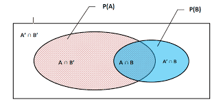
A pair of random variables $(X, Y)$ is said to be independent if for any $A$ and $B$,
$$
p(X \in A \mid Y \in B)=p(X \in A),
$$
or alternatively $p(Y \in B \mid X \in A)=p(Y \in B)$ (these two definitions are correct and equivalent under very mild conditions that prevent ill-formed conditioning on an event that has zero probability).

Using the chain rule, it can also be shown that the above two definitions are equivalent to the requirement that $p(X \in A, Y \in B)=p(X \in A) p(Y \in B)$ for all $A$ and $B$.

Independence between random variables implies that the random variables do not provide information about each other. This means that knowing the value of $X$ does not help us infer anything about the value of $Y$-in other words, it does not change the probability of $Y$. (Or vice-versa $-Y$ does not tell us anything about $X$.) While independence is an important concept in probability and statistics, in this book we will more frequently make use of a more refined notion of independence, called “conditional independence”-which is a generalization of the notion of independence described in the beginning of this section. A pair of random variables $(X, Y)$ is conditionally independent given a third random variable $Z$, if for any $A, B$ and $z$, it holds that $p(X \in A \mid Y \in B, Z=z)=p(X \in A \mid Z=z)$.

Conditional independence between two random variables (given a third one) implies that the two variables are not informative about each other, if the value of the third one is known. 3
Conditional independence (and independence) can be generalized to multiple random variables as well. We say that a set of random variables $X_{1}, \ldots, X_{n}$, are mutually conditionally independent given another set of random variables $Z_{1}, \ldots, Z_{m}$ if the following applies for any $A_{1}, \ldots, A_{n}$ and $z_{1}, \ldots, z_{m}:$
$$
\begin{gathered}
p\left(X_{1} \in A_{1}, \ldots, X_{n} \in A_{n} \mid Z_{1}=z_{1}, \ldots, Z_{m}=z_{m}\right)= \
\prod_{i=1}^{n} p\left(X_{i} \in A_{i} \mid Z_{1}=z_{1}, \ldots, Z_{m}=z_{m}\right) .
\end{gathered}
$$
This type of independence is weaker than pairwise independence for a set of random variables, in which only pairs of random variables are required to be independent. (Also see exercises.)

统计代写|贝叶斯分析代写Bayesian Analysis代考|EXCHANGEABLE RANDOM VARIABLES

Another type of relationship that can be present between random variables is that of exchangeability. A sequence of random variables $X_{1}, X_{2}, \ldots$ over $\Omega$ is said to be exchangeable, if for any finite subset, permuting the random variables in this finite subset, does not change their joint distribution. More formally, for any $S=\left{a_{1}, \ldots, a_{m}\right}$ where $a_{i} \geq 1$ is an integer, and for any permutation $\pi$ on ${1, \ldots, m}$, it holds that: ${ }^{4}$
$$
p\left(x_{a_{1}}, \ldots, x_{a_{m}}\right)=p\left(x_{a_{\pi(1)}}, \ldots, x_{\left.a_{\pi(m)}\right)}\right) .
$$
Due to a theorem by de Finetti (Finetti, 1980), exchangeability can be thought of as meaning “conditionally independent and identically distributed” in the following sense. De Finetti showed that if a sequence of random variables $X_{1}, X_{2}, \ldots$ is exchangeable, then under some regularity conditions, there exists a sample space $\Theta$ and a distribution over $\Theta, p(\theta)$, such that:
$$
p\left(X_{a_{1}}, \ldots, X_{a_{m}}\right)=\int_{\theta} \prod_{i=1}^{m} p\left(X_{a_{i}} \mid \theta\right) p(\theta) d \theta,
$$
for any set of $m$ integers, $\left{a_{1}, \ldots, a_{m}\right}$. The interpretation of this is that exchangeable random variables can be represented as a (potentially infinite) mixture distribution. This theorem is also called the “representation theorem.”

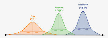
The frequentist approach assumes the existence of a fixed set of parameters from which the data were generated, while the Bayesian approach assumes that there is some prior distribution over the set of parameters that generated the data. (This will hecome clearer as the hook progresses.) De Finetti’s theorem provides another connection between the Bayesian approach and the frequentist one. The standard “independent and identically distributed” (i.i.d.) assumption in the frequentist setup can be asserted as a setup of exchangeability where $p(\theta)$ is a point-mass distribution over the unknown (but single) parameter from which the data are sampled. This leads to the observations being unconditionally independent and identically distributed. In the Bayesian setup, however, the observations are correlated, because $p(\theta)$ is not a point-mass distribution. The prior distribution plays the role of $p(\theta)$. For a detailed discussion of this similarity, see O’Neill (2009).

统计代写|贝叶斯分析代写Bayesian Analysis代考|EXPECTATIONS OF RANDOM VARIABLES

If we consider again the naive definition of random variables, as functions that map the sample space to real values, then it is also useful to consider various ways in which we can summarize these random variables. One way to get a summary of a random variable is by computing its expectation, which is its weighted mean value according to the underlying probability model.
It is easiest to first consider the expectation of a continuous random variable with a density function. Say $p(\theta)$ defines a distribution over the random variable $\theta$, then the expectation of $\theta$, denoted $E[\theta]$ would be defined as:
$$
E[\theta]=\int_{\theta} p(\theta) \theta d \theta .
$$
For the discrete random variables that we consider in this book, we usually consider expectations of functions over these random variables. As mentioned in Section 1.2, discrete random variable values often range over a set which is not numeric. In these cases, there is no “mean value” for the values that these random variables accept. Instead, we will compute the mean value of a real-function of these random variables.
With $f$ being such a function, the expectation $E[f(X)]$ is defined as:
$$
E[f(X)]=\sum_{x} p(x) f(x)
$$ For the linguistic structures that are used in this book, we will often use a function $f$ that indicates whether a certain property holds for the structure. For example, if the sample space of $X$ is a set of sentences, $f(x)$ can be an indicator function that states whether the word “spring” appears in the sentence $x$ or not; $f(x)=1$ if the word “spring” appears in $x$ and 0 , otherwise. In that case, $f(X)$ itself can be thought of as a Bernoulli random variable, i.e., a binary random variable that has a certain probability $\theta$ to be 1 , and probability $1-\theta$ to be 0 . The expectation $E[f(X)]$ gives the probability that this random variable is 1 . Alternatively, $f(x)$ can count how many times the word “spring” appears in the sentence $x$. In that case, it can be viewed as a sum of Bernoulli variables, each indicating whether a certain word in the sentence $x$ is “spring” or not.

贝叶斯分析代考

统计代写|贝叶斯分析代写Bayesian Analysis代考|INDEPENDENT AND CONDITIONALLY INDEPENDENT

一对随机变量 $(X, Y)$ 据说是独立的，如果有的话 $A$ 和 $B$ ，
$$
p(X \in A \mid Y \in B)=p(X \in A),
$$
或者 $p(Y \in B \mid X \in A)=p(Y \in B)$ (这两个定义在非常温和的条件下是正确且等效的，可以防止对概率为零的事件进行不良条件反射) 。
使用链式法则，也可以证明上述两个定义等价于: $p(X \in A, Y \in B)=p(X \in A) p(Y \in B)$ 对所有人 $A$ 和 $B$.
随机变量之间的独立性意味着随机变量不提供关于彼此的信息。这意味着知道 $X$ 并不能帮助我们推断出任何关于 $Y$ – 换句话说，它不会改变 $Y$. (或相反亦然 $-Y$ 没有告诉我们任何关于 $X$.) 虽然独立性是概率和统计学中的一个重要概念，但在本书中，我们将更频做地使用一个更精炼的独立性概念，称为”条件独立性”一一它是对本书开头描述的独立性概念的概括。本节。一对随机变量 $(X, Y)$ 给定第三个随机变量条件独立 $Z$, 如果有的话 $A, B$ 和 $z$, 它认为 $p(X \in A \mid Y \in B, Z=z)=p(X \in A \mid Z=z)$.
两个随机变量之间的条件独立性（给定第三个）意味着如果第三个变量的值已知，则这两个变量不会相互提供信息。 3
条件独立性（和独立性）也可以推广到多个随机变量。我们说一组随机变量 $X_{1}, \ldots, X_{n}$ ，在给定另一组随机变量的情况下相互条件独立 $Z_{1}, \ldots, Z_{m}$ 如果以下适用于任何 $A_{1}, \ldots, A_{n}$ 和 $z_{1}, \ldots, z_{m}$ :
$$
p\left(X_{1} \in A_{1}, \ldots, X_{n} \in A_{n} \mid Z_{1}=z_{1}, \ldots, Z_{m}=z_{m}\right)=\prod_{i=1}^{n} p\left(X_{i} \in A_{i} \mid Z_{1}=z_{1}, \ldots, Z_{m}=z_{m}\right) \text {. }
$$
这种类型的独立性弱于一组随机变量的成对独立性，其中只要求成对的随机变量是独立的。（另见练习。）

统计代写|贝叶斯分析代写Bayesian Analysis代考|EXCHANGEABLE RANDOM VARIABLES

随机变量之间可能存在的另一种关系是可交换性。一系列随机变量 $X_{1}, X_{2}, \ldots$ 超过 $\Omega$ 据说是可交换的，如果对于任何有限子集，置换该有限子集中的随机变量，不会改变它们的联合分布。更正式地说，对于任何
$\mathrm{S}=|$ left{a_{1}，Vdots, a_{m}|right} 在哪里 $a_{i} \geq 1$ 是一个整数，并且对于任何排列 $\pi$ 上 $1, \ldots, m$ ，它认为: ${ }^{4}$
$$
p\left(x_{a_{1}}, \ldots, x_{a_{m}}\right)=p\left(x_{a_{\pi(1)}}, \ldots, x_{\left.a_{\pi(m)}\right)}\right) .
$$
由于 de Finetti (Finetti, 1980) 的一个定理，可交换性可以被认为是以下意义上的“条件独立且同分布”。De Finetti 证明，如果一系列随机变量 $X_{1}, X_{2}, \ldots$ 是可交换的，那么在一定的规律性条件下，存在一个样本空间 $\Theta$ 和分布 $\Theta, p(\theta)$, 这样:
$$
p\left(X_{a_{1}}, \ldots, X_{a_{m i}}\right)=\int_{\theta} \prod_{i=1}^{m} p\left(X_{a_{i}} \mid \theta\right) p(\theta) d \theta
$$
对于任何一组 $m$ 整数， Ileft{a_{1}, Idots, a_{m}\right}. 对此的解释是可交换随机变量可以表示为（可能是无限的) 混合分布。该定理也称为“表示定理”。
常客方法假设存在一组固定的参数，从这些参数中生成数据，而贝叶斯方法假设在生成数据的参数集上存在一些先验分布。(随着钩子的进行，这将变得更加清晰。) 德菲内蒂定理提供了贝叶斯方法和常客方法之间的另一种联系。常客设置中的标准”独立同分布” (iid) 假设可以断言为可交换性设置，其中 $p(\theta)$ 是从其中采样数据的末知 (但单一) 参数上的点质量分布。这导致观察结果是无条件独立且同分布的。然而，在贝叶斯设置中，观察结果是相关的，因为 $p(\theta)$ 不是点质量分布。先验分布的作用是 $p(\theta)$. 有关这种相似性的详细讨论，请参见 O’Neill (2009)。

统计代写|贝叶斯分析代写Bayesian Analysis代考|EXPECTATIONS OF RANDOM VARIABLES

如果我们再次考虑随机变量的朴素定义，作为将样本空间映射到真实值的函数，那么考虑总结这些随机变量的各种方式也是有用的。获得随机变量摘要的一种方法是计算其期望值，即根据潜在概率模型的加权平均值。
首先考虑具有密度函数的连续随机变量的期望是最容易的。说 $p(\theta)$ 定义随机变量的分布 $\theta$ ，那么期望 $\theta$ ，表示 $E[\theta]$ 将被定义为:
$$
E[\theta]=\int_{\theta} p(\theta) \theta d \theta
$$
对于我们在本书中考虑的离散随机变量，我们通常会考虑函数对这些随机变量的期望。如 $1.2$ 节所述，离散随机变量值通常在一个非数字的集合上。在这些情况下，这些随机变量接受的值没有“平均值”。相反，我们将计算这些随机变量的实函数的平均值。
和 $f$ 作为这样的功能，期望 $E[f(X)]$ 定义为:
$$
E[f(X)]=\sum_{x} p(x) f(x)
$$
对于本书中使用的语言结构，我们通常会使用一个函数 $f$ 这表明某个属性是否适用于该结构。例如，如果样本空间 $X$ 是一组句子， $f(x)$ 可以是一个指示函数，表明句子中是否出现了”spring”这个词 $x$ 或不: $f(x)=1$ 如果“春天”这个词出现在 $x$ 和 0 ，否则。在这种情况下， $f(X)$ 本身可以认为是伯努利随机变量，即具有一定概率的二元随机变量 $\theta$ 为 1 和概率 $1-\theta$ 为 0 。期望 $E[f(X)]$ 给出此随机变量为 1 的概率. 或者， $f(x)$ 可以数出“spring”这个词在句子中出现了多少次 $x$. 在那种情况下，它可以看作是伯努利变量的总和，每个变量表示句子中的某个词是否 $x$ 是不是 “春天”。

统计代写|贝叶斯分析代写Bayesian Analysis代考请认准statistics-lab™

统计代写请认准statistics-lab™. statistics-lab™为您的留学生涯保驾护航。

金融工程代写

金融工程是使用数学技术来解决金融问题。金融工程使用计算机科学、统计学、经济学和应用数学领域的工具和知识来解决当前的金融问题，以及设计新的和创新的金融产品。

非参数统计代写

非参数统计指的是一种统计方法，其中不假设数据来自于由少数参数决定的规定模型；这种模型的例子包括正态分布模型和线性回归模型。

广义线性模型代考

广义线性模型（GLM）归属统计学领域，是一种应用灵活的线性回归模型。该模型允许因变量的偏差分布有除了正态分布之外的其它分布。

术语广义线性模型（GLM）通常是指给定连续和/或分类预测因素的连续响应变量的常规线性回归模型。它包括多元线性回归，以及方差分析和方差分析（仅含固定效应）。

有限元方法代写

有限元方法（FEM）是一种流行的方法，用于数值解决工程和数学建模中出现的微分方程。典型的问题领域包括结构分析、传热、流体流动、质量运输和电磁势等传统领域。

有限元是一种通用的数值方法，用于解决两个或三个空间变量的偏微分方程（即一些边界值问题）。为了解决一个问题，有限元将一个大系统细分为更小、更简单的部分，称为有限元。这是通过在空间维度上的特定空间离散化来实现的，它是通过构建对象的网格来实现的：用于求解的数值域，它有有限数量的点。边界值问题的有限元方法表述最终导致一个代数方程组。该方法在域上对未知函数进行逼近。[1] 然后将模拟这些有限元的简单方程组合成一个更大的方程系统，以模拟整个问题。然后，有限元通过变化微积分使相关的误差函数最小化来逼近一个解决方案。

tatistics-lab作为专业的留学生服务机构，多年来已为美国、英国、加拿大、澳洲等留学热门地的学生提供专业的学术服务，包括但不限于Essay代写，Assignment代写，Dissertation代写，Report代写，小组作业代写，Proposal代写，Paper代写，Presentation代写，计算机作业代写，论文修改和润色，网课代做，exam代考等等。写作范围涵盖高中，本科，研究生等海外留学全阶段，辐射金融，经济学，会计学，审计学，管理学等全球99%专业科目。写作团队既有专业英语母语作者，也有海外名校硕博留学生，每位写作老师都拥有过硬的语言能力，专业的学科背景和学术写作经验。我们承诺100%原创，100%专业，100%准时，100%满意。

随机分析代写

随机微积分是数学的一个分支，对随机过程进行操作。它允许为随机过程的积分定义一个关于随机过程的一致的积分理论。这个领域是由日本数学家伊藤清在第二次世界大战期间创建并开始的。

时间序列分析代写

随机过程，是依赖于参数的一组随机变量的全体，参数通常是时间。随机变量是随机现象的数量表现，其时间序列是一组按照时间发生先后顺序进行排列的数据点序列。通常一组时间序列的时间间隔为一恒定值（如1秒，5分钟，12小时，7天，1年），因此时间序列可以作为离散时间数据进行分析处理。研究时间序列数据的意义在于现实中，往往需要研究某个事物其随时间发展变化的规律。这就需要通过研究该事物过去发展的历史记录，以得到其自身发展的规律。

回归分析代写

多元回归分析渐进（Multiple Regression Analysis Asymptotics）属于计量经济学领域，主要是一种数学上的统计分析方法，可以分析复杂情况下各影响因素的数学关系，在自然科学、社会和经济学等多个领域内应用广泛。

MATLAB代写

MATLAB 是一种用于技术计算的高性能语言。它将计算、可视化和编程集成在一个易于使用的环境中，其中问题和解决方案以熟悉的数学符号表示。典型用途包括：数学和计算算法开发建模、仿真和原型制作数据分析、探索和可视化科学和工程图形应用程序开发，包括图形用户界面构建MATLAB 是一个交互式系统，其基本数据元素是一个不需要维度的数组。这使您可以解决许多技术计算问题，尤其是那些具有矩阵和向量公式的问题，而只需用 C 或 Fortran 等标量非交互式语言编写程序所需的时间的一小部分。MATLAB 名称代表矩阵实验室。MATLAB 最初的编写目的是提供对由 LINPACK 和 EISPACK 项目开发的矩阵软件的轻松访问，这两个项目共同代表了矩阵计算软件的最新技术。MATLAB 经过多年的发展，得到了许多用户的投入。在大学环境中，它是数学、工程和科学入门和高级课程的标准教学工具。在工业领域，MATLAB 是高效研究、开发和分析的首选工具。MATLAB 具有一系列称为工具箱的特定于应用程序的解决方案。对于大多数 MATLAB 用户来说非常重要，工具箱允许您学习和应用专业技术。工具箱是 MATLAB 函数（M 文件）的综合集合，可扩展 MATLAB 环境以解决特定类别的问题。可用工具箱的领域包括信号处理、控制系统、神经网络、模糊逻辑、小波、仿真等。

R语言代写	问卷设计与分析代写
PYTHON代写	回归分析与线性模型代写
MATLAB代写	方差分析与试验设计代写
STATA代写	机器学习/统计学习代写
SPSS代写	计量经济学代写
EVIEWS代写	时间序列分析代写
EXCEL代写	深度学习代写
SQL代写	各种数据建模与可视化代写

统计代写|贝叶斯分析代写Bayesian Analysis代考|MSH3

Posted on 2022年6月30日2022年6月30日 by statistics-lab

如果你也在怎样代写贝叶斯分析Bayesian Analysis这个学科遇到相关的难题，请随时右上角联系我们的24/7代写客服。

我们提供的贝叶斯分析Bayesian Analysis及其相关学科的代写，服务范围广, 其中包括但不限于:

Statistical Inference 统计推断
Statistical Computing 统计计算
Advanced Probability Theory 高等概率论
Advanced Mathematical Statistics 高等数理统计学
(Generalized) Linear Models 广义线性模型
Statistical Machine Learning 统计机器学习
Longitudinal Data Analysis 纵向数据分析
Foundations of Data Science 数据科学基础

统计代写|贝叶斯分析代写Bayesian Analysis代考|JOINT DISTRIBUTION OVER MULTIPLE RANDOM VARIABLES

It is possible to define several random variables on the same sample space. For example, for a discrete sample space, such as a set of words, we can define two random variables $X$ and $Y$ that take integer values-one could measure word length and the other could measure the count of vowels in a word. Given two such random variables, the joint distribution $P(X, Y)$ is a function that maps pairs of events $(A, B)$ as follows:
$$
p(X \in A, Y \in B)=p\left(X^{-1}(A) \cap Y^{-1}(B)\right)
$$
It is often the case that we take several sets $\left{\Omega_{1}, \ldots, \Omega_{m}\right}$ and combine them into a single sample space $\Omega=\Omega_{1} \times \ldots \times \Omega_{m}$. Each of the $\Omega_{i}$ is associated with a random variable. Based on this, a joint probability distribution can be defined for all of these random variables together. For example, consider $\Omega=V \times P$ where $V$ is a vocabulary of words and $P$ is a part-of-speech tag. This sample space enables us to define probabilities $p(x, y)$ where $X$ denotes a word associated with a part of speech $Y$. In this case, $x \in V$ and $y \in P$.

With any joint distribution, we can marginalize some of the random variables to get a distribution which is defined over a subset of the original random variables (so it could still be a joint distribution, only over a subset of the random variables). Marginalization is done using integration (for continuous variables) or summing (for discrete random variables). This operation of summation or integration eliminates the random variable from the joint distribution. The result is a joint distribution over the non-marginalized random variables.

For the simple part-of-speech example above, we could either get the marginal $p(x)=$ $\sum_{y \in P} p(x, y)$ or $p(y)=\sum_{x \in V} p(x, y)$. The marginals $p(X)$ and $p(Y)$ do not uniquely determine the joint distribution value $p(X, Y)$. Only the reverse is true. However, whenever $X$ and $Y$ are independent then the joint distribution can be determined using the marginals. More about this in Section 1.3.2.

统计代写|贝叶斯分析代写Bayesian Analysis代考|CONDITIONAL DISTRIBUTIONS

Joint probability distributions provide an answer to questions about the probability of several random variables to obtain specific values. Conditional distributions provide an answer to a different, but related question. They help to determine the values that a random variable can obtain, when other variables in the joint distribution are restricted to specific values (or when they are “clamped”).

Conditional distributions are derivable from joint distributions over the same set of random variables. Consider a pair of random variables $X$ and $Y$ (either continuous or discrete). If $A$ is an event from the sample space of $X$ and $y$ is a value in the sample space of $Y$, then:
$$
p(X \in A \mid Y=y)=\frac{p(X \in A, Y=y)}{p(Y=y)}
$$
is to be interpreted as a conditional distribution that determines the probability of $X \in A$ conditioned on $Y$ obtaining the value $y$. The bar denotes that we are clamping $Y$ to the value $y$ and identifying the distribution induced on $X$ in the restricted sample space. Informally, the conditional distribution takes the part of the sample space where $Y=y$ and re-normalizes the joint distribution such that the result is a probability distribution defined only over that part of the sample space.

When we consider the joint distribution in Equation $1.1$ to be a function that maps events to probabilities in the space of $X$, with $y$ being fixed, we note that the value of $p(Y=y)$ is actually a normalization constant that can be determined from the numerator $p(X \in A, Y=y)$. For example, if $X$ is discrete when using a PMF, then:
$$
p(Y=y)=\sum_{x} p(X=x, Y=y) .
$$

统计代写|贝叶斯分析代写Bayesian Analysis代考|BAYES’ RULE

Bayes’ rule is a basic result in probability that describes a relationship between two conditional distributions $p(X \mid Y)$ and $p(Y \mid X)$ for a pair of random variables (these random variables can also be continuous). More specifically, Bayes’ rule states that for any such pair of random variables, the following identity holds:
$$
p(Y=y \mid X=x)=\frac{p(X-x \mid Y-y) p(Y-y)}{p(X=x)}
$$

This result also generally holds true for any two events $A$ and $B$ with the conditional probability $p(X \in A \mid Y \in B)$.

The main advantage that Bayes’ rule offers is inversion of the conditional relationship between two random variables – therefore, if one variable is known, then the other can be calculated as well, assuming the marginal distributions $p(X=x)$ and $p(Y=y)$ are also known.
Bayes’ rule can be proven in several ways. One way to derive it is simply by using the chain rule twice. More specifically, we know that the joint distribution values can be rewritten as follows, using the chain rule, either first separating $X$ or first separating $Y$ :
$$
\begin{aligned}
p(X&=x, Y=y) \
&=p(X=x) p(Y=y \mid X=x) \
&=p(Y=y) p(X=x \mid Y=y)
\end{aligned}
$$
Taking the last equality above, $p(X=x) p(Y=y \mid X=x)=p(Y=y) p(X=x \mid Y=$ $y)$, and dividing both sides by $p(X=x)$ results in Bayes’ rule as described in Equation 1.2.
Bayes’ rule is the main pillar in Bayesian statistics for reasoning and learning from data. Bayes’ rule can invert the relationship between “observations” (the data) and the random variables we are interested in predicting. This makes it possible to infer target predictions from such observations. A more detailed description of these ideas is provided in Section 1.5, where statistical modeling is discussed.

贝叶斯分析代考

统计代写|贝叶斯分析代写Bayesian Analysis代考|JOINT DISTRIBUTION OVER MULTIPLE RANDOM VARIABLES

可以在同一个样本空间上定义多个随机变量。例如，对于一个离散的样本空间，比如一组词，我们可以定义两个随机变量 $X$ 和 $Y$ 取整数值一一一个可以测量单词长度，另一个可以测量单词中元音的数量。给定两个这样的随机变量，联合分布 $P(X, Y)$ 是映射成对事件的函数 $(A, B)$ 如下:
$$
p(X \in A, Y \in B)=p\left(X^{-1}(A) \cap Y^{-1}(B)\right)
$$
$\mathrm{~ 我们经常会采取几组 ~ V e f t { 1 O m e g a _ { 1 } , ~ \ d o t s , ~ I O m e g a _ { m }}$ $\Omega=\Omega_{1} \times \ldots \times \Omega_{m}$. 每个 $\Omega_{i}$ 与随机变量相关联。基于此，可以为所有这些随机变量一起定义联合概率分布。例如，考虑 $\Omega=V \times P$ 在哪里 $V$ 是一个词汇表和 $P$ 是词性标签。这个样本空间使我们能够定义概率 $p(x, y)$ 在哪里 $X$ 表示与词性相关的词 $Y$. 在这种情况下， $x \in V$ 和 $y \in P$.
对于任何联合分布，我们可以边缘化一些随机变量以获得在原始随机变量的子集上定义的分布（因此它仍然可以是联合分布，仅在随机变量的子集上)。使用积分 (对于连续变量) 或求和 (对于离散随机变量) 进行边缘化。这种求和或积分操作从联合分布中消除了随机变量。结果是非边缘化随机变量的联合分布。
对于上面简单的词性示例，我们可以得到边缘 $p(x)=\sum_{y \in P} p(x, y)$ 或者 $p(y)=\sum_{x \in V} p(x, y)$. 边缘人 $p(X)$ 和 $p(Y)$ 不唯一确定联合分布值 $p(X, Y)$. 只有反过来才是正确的。然而，每当 $X$ 和 $Y$ 是独立的，则可以使用边际确定联合分布。在第 $1.3 .2$ 节中了解更多信息。

统计代写|贝叶斯分析代写Bayesian Analysis代考|CONDITIONAL DISTRIBUTIONS

联合概率分布为有关几个随机变量获得特定值的概率问题提供了答案。条件分布为不同但相关的问题提供了答案。当联合分布中的其他变量被限制为特定值时（或当它们被”钅制”时），它们有助于确定随机变量可以获得的值。
条件分布可从同一组随机变量上的联合分布推导出来。考虑一对随机变量 $X$ 和 $Y$ (连续的或离散的)。如果 $A$ 是来自样本空间的事件 $X$ 和 $y$ 是样本空间中的一个值 $Y$ ，然后：
$$
p(X \in A \mid Y=y)=\frac{p(X \in A, Y=y)}{p(Y=y)}
$$
将被解释为确定概率的条件分布 $X \in A$ 以 $Y$ 获取价值 $y$. 条形表示我们正在夹紧 $Y$ 到价值 $y$ 并确定引起的分布 $X$ 在有限的样本空间中。非正式地，条件分布占据样本空间的一部分，其中 $Y=y$ 并重新归一化联合分布，使得结果是仅在样本空间的该部分上定义的概率分布。
当我们考虑方程中的联合分布时 $1.1$ 是一个将事件映射到空间中的概率的函数 $X$ ，和 $y$ 是固定的，我们注意到，价值 $p(Y=y)$ 实际上是一个归一化常数，可以从分子中确定 $p(X \in A, Y=y)$. 例如，如果 $X$ 使用 PMF 时是离散的，则:
$$
p(Y=y)=\sum_{x} p(X=x, Y=y)
$$

统计代写|贝叶斯分析代写Bayesian Analysis代考|BAYES’ RULE

贝叶斯规则是描述两个条件分布之间关系的概率的基本结果 $p(X \mid Y)$ 和 $p(Y \mid X)$ 对于一对随机变量 (这些随机变量也可以是连续的）。更具体地说，贝叶斯规则指出，对于任何这样的随机变量对，以下恒等式成立：
$$
p(Y=y \mid X=x)=\frac{p(X-x \mid Y-y) p(Y-y)}{p(X=x)}
$$
这个结果通常也适用于任何两个事件 $A$ 和 $B$ 有条件概率 $p(X \in A \mid Y \in B)$.
贝叶斯规则提供的主要优点是反转两个随机变量之间的条件关系一一因此，如果一个变量是已知的，那么假设边际分布也可以计算另一个变量 $p(X=x)$ 和 $p(Y=y)$ 也是众所周知的。
贝叶斯规则可以通过多种方式证明。推导它的一种方法是简单地使用链式法则两次。更具体地说，我们知道联合分布值可以改写如下，使用链式法则，或者首先分离 $X$ 或先分离 $Y:$
$$
p(X=x, Y=y) \quad=p(X=x) p(Y=y \mid X=x)=p(Y=y) p(X=x \mid Y=y)
$$
取上面最后一个等式， $p(X=x) p(Y=y \mid X=x)=p(Y=y) p(X=x \mid Y=y)$ ，并将两边除以 $p(X=x)$ 得出公式 $1.2$ 中描述的贝叶斯规则。
贝叶斯规则是贝叶斯统计中用于推理和从数据中学习的主要支柱。贝叶斯规则可以颠倒“观察”（数据）和我们有兴趣预测的随机变量之间的关系。这使得从这些观察中推断出目标预测成为可能。1.5节提供了对这些想法的更详细描述，其中讨论了统计建模。

统计代写请认准statistics-lab™. statistics-lab™为您的留学生涯保驾护航。

金融工程代写

非参数统计代写

非参数统计指的是一种统计方法，其中不假设数据来自于由少数参数决定的规定模型；这种模型的例子包括正态分布模型和线性回归模型。

广义线性模型代考

广义线性模型（GLM）归属统计学领域，是一种应用灵活的线性回归模型。该模型允许因变量的偏差分布有除了正态分布之外的其它分布。

有限元方法代写

随机分析代写

时间序列分析代写

回归分析代写

MATLAB代写

R语言代写	问卷设计与分析代写
PYTHON代写	回归分析与线性模型代写
MATLAB代写	方差分析与试验设计代写
STATA代写	机器学习/统计学习代写
SPSS代写	计量经济学代写
EVIEWS代写	时间序列分析代写
EXCEL代写	深度学习代写
SQL代写	各种数据建模与可视化代写

统计代写|贝叶斯分析代写Bayesian Analysis代考|DATA5711

Posted on 2022年6月30日2022年6月30日 by statistics-lab

如果你也在怎样代写贝叶斯分析Bayesian Analysis这个学科遇到相关的难题，请随时右上角联系我们的24/7代写客服。

我们提供的贝叶斯分析Bayesian Analysis及其相关学科的代写，服务范围广, 其中包括但不限于:

Statistical Inference 统计推断
Statistical Computing 统计计算
Advanced Probability Theory 高等概率论
Advanced Mathematical Statistics 高等数理统计学
(Generalized) Linear Models 广义线性模型
Statistical Machine Learning 统计机器学习
Longitudinal Data Analysis 纵向数据分析
Foundations of Data Science 数据科学基础

统计代写|贝叶斯分析代写Bayesian Analysis代考|DATA5711

统计代写|贝叶斯分析代写Bayesian Analysis代考|PROBABILITY MEASURES

At the core of probabilistic theory (and probabilistic modeling) lies the idea of a “sample space.” The sample space is a set $\Omega$ that consists of all possible elements over which we construct a probability distribution. In this book, the sample space most often consists of objects relating to language, such as words, phrase-structure trees, sentences, documents or sequences. As we see later, in the Bayesian setting, the sample space is defined to be a Cartesian product between a set of such objects and a set of model parameters (Section 1.5.1).

Once a sample space is determined, we can define a probability measure for that sample space. A probability measure $p$ is a function which attaches a real number to events-subsets of the sample space.
A probability measure has to satisfy three axiomatic properties:

It has to be a non-negative function such that $p(A) \geq 0$ for any event $A$.
For any countable disjoint sequence of events $A_{i} \subseteq \Omega, i \in{1, \ldots}$, if $A_{i} \cap A_{j}=\emptyset$ for $i \neq$ $j$, it should hold that $p\left(\bigcup_{i} A_{i}\right)=\sum_{i} p\left(A_{i}\right)$. This means that the sum of probabilities of disjoint events should equal the probability of the union of the events.
The probability of $\Omega$ is $1: p(\Omega)=1$.

There are a few consequences from these three axiomatic properties. The first is that $p(\emptyset)=0$ (to see this, consider that $p(\Omega)+p(\emptyset)=p(\Omega \cup \emptyset)=p(\Omega)=1$ ). The second is that $p(A \cup B)=p(A)+p(B)-p(A \cap B)$ for any two events $A$ and $B$ (to see this, consider that $p(A \cup B)=p(A)+p(B \backslash(A \cap B))$ and that $p(B)=p(B \backslash(A \cap B))+p(A \cap B))$. And finally, the complement of an event $A, \Omega \backslash A$ is such that $p(\Omega \backslash A)=1-p(A)$ (to see this, consider that $1=p(\Omega)=p((\Omega \backslash A) \cup A)=p(\Omega \backslash A)+p(A)$ for any event $A)$.

In the general case, not every subset of the sample space should be considered an event.
From a measure-theoretic point of view for probability theory, an event must be a “measurable set.” The collection of measurable sets of a given sample space needs to satisfy some axiomatic properties. ${ }^{1}$ A discussion of measure theory is beyond the scope of this book, but see Ash and Doléans-Dade (2000) for a thorough investigation of this topic.

For our discrete sample spaces, consisting of linguistic structures or other language-related discrete objects, this distinction of measurable sets from arbitrary subsets of the sample space is not crucial. We will consider all subsets of the sample space to be measurable, which means they could be used as events. For continuous spaces, we will be using well-known probability measures that rely on Lebesgue’s measure. This means that the sample space will be a subset of a Euclidean space, and the set of events will be the subsets of this space that can be integrated over using Lebesgue’s integration.

统计代写|贝叶斯分析代写Bayesian Analysis代考|RANDOM VARIABLES

In their most basic form, random variables are functions that map each $w \in \Omega$ to a real value. They are often denoted by capital letters such as $X$ and $Z$. Once such a function is defined, under some regularity conditions, it induces a probability measure over the real numbers. More specifically, for any $A \subseteq \mathbb{R}$ such that the pre-image, $X^{-1}(A)$, defined as, ${\omega \in \Omega \mid X(\omega) \in A}$, is an event, its probability is:
$$
p_{X}(A)=p(X \in A)=p\left(X^{-1}(A)\right),
$$
where $p_{X}$ is the probability measure induced by the random variable $X$ and $p$ is a probability measure originally defined for $\Omega$. The sample space for $p_{X}$ is $\mathbb{R}$. The set of events for this sample space includes all $A \subseteq \mathbb{R}$ such that $X^{-1}(A)$ is an event in the original sample space $\Omega$ of $p$.
It is common to define a statistical model directly in terms of random variables, instead of explicitly defining a sample space and its corresponding real-value functions. In this case, random variables do not have to be interpreted as real-value functions and the sample space is understood to be a range of the random variable function. For example, if one wants to define a probability distribution over a language vocabulary, then one can define a random variable $X(\omega)=\omega$ with $\omega$ ranging over words in the vocabulary. Following this, the probability of a word in the vocabulary is denoted by $p(X \in{\omega})=p(X=\omega)$.

统计代写|贝叶斯分析代写Bayesian Analysis代考|CONTINUOUS AND DISCRETE RANDOM VARIABLES

This book uses the two most common kinds of random variables available in statistics: continuous and discrete. Continuous random variables take values in a continuous space, usually a subspace of $\mathbb{R}^{d}$ for $d \geq 1$. Discrete random variables, on the other hand, take values from a discrete, possibly countable set. In this book, discrete variables are usually denoted using capital letters such as $X, Y$ and $Z$, while continuous variables are denoted using greek letters, such as $\theta$ and $\mu$.

The continuous variables in this book are mostly used to define a prior over the parameters of a discrete distribution, as is usually done in the Bayesian setting. See Section $1.5 .2$ for a discussion of continuous variables. The discrete variables, on the other hand, are used to model structures that will be predicted (such as parse trees, part-of-speech tags, alignments, clusters) or structures which are observed (such as a sentence, a string over some language vocabulary or other such sequences).

The discrete variables discussed in this book are assumed to have an underlying probability mass function (PMF)-i.e., a function that attaches a weight to each element in the sample space, $p(x)$. This probability mass function induces the probability measure $p(X \in A)$, which satisfies:
$$
p(X \in A)=\sum_{x \in A} p(x),
$$
where $A$ is a subset of the possible values $X$ can take. Note that this equation is the result of the axiom of probability measures, where the probability of an event equals the sum of probabilities of disjoint events that precisely cover that event (singletons, in our case).

贝叶斯分析代考

统计代写|贝叶斯分析代写Bayesian Analysis代考|PROBABILITY MEASURES

概率论 (和概率建模) 的核心是“样本空间”的概念。样本空间是一个集合 $\Omega$ 它由我们构建概率分布的所有可能元素组成。在本书中，样本空间通常由与语言相关的对象组成，例如单词、短语结构树、句子、文档或序列。正如我们稍后看到的，在贝叶斯设置中，样本空间被定义为一组此类对象和一组模型参数之间的笛卡尔积 (第 $1.5 .1$ 节) 。
一旦确定了样本空间，我们就可以为该样本空间定义概率测度。概率测度 $p$ 是一个将实数附加到样本空间的事件子集的函数。
概率度量必须满足三个公理性质:

它必须是一个非负函数，使得 $p(A) \geq 0$ 对于任何事件 $A$.
对于任何可数的不相交的事件序列 $A_{i} \subseteq \Omega, i \in 1, \ldots$ ，如果 $A_{i} \cap A_{j}=\emptyset$ 为了 $i \neq j$ ，它应该认为 $p\left(\bigcup_{i} A_{i}\right)=\sum_{i} p\left(A_{i}\right)$. 这意味着不相交事件的概率之和应该等于事件联合的概率。
的概率 $\Omega$ 是 $1: p(\Omega)=1$.
这三个公理性质有一些结果。第一个是 $p(\emptyset)=0$ (要看到这一点，请考虑
$p(\Omega)+p(\emptyset)=p(\Omega \cup \emptyset)=p(\Omega)=1)$ 。第二个是 $p(A \cup B)=p(A)+p(B)-p(A \cap B)$ 对于任何两个事件 $A$ 和 $B$ (要看到这一点，请考虑 $p(A \cup B)=p(A)+p(B \backslash(A \cap B))$ 然后
$p(B)=p(B \backslash(A \cap B))+p(A \cap B))$. 最后，事件的补充 $A, \Omega \backslash A$ 是这样的 $p(\Omega \backslash A)=1-p(A)$ (要看到这一点，请考虑 $1=p(\Omega)=p((\Omega \backslash A) \cup A)=p(\Omega \backslash A)+p(A)$ 对于任何事件 $A)$.
在一般情况下，并非样本空间的每个子集都应被视为一个事件。
从概率论的测度论观点来看，一个事件必须是一个”可测集”。给定样本空间的可测量集的集合需要满足一些公理性质。 1 测度论的讨论超出了本书的范围，但请参阅 Ash 和 Doléans-Dade (2000) 对该主题的深入研究。
对于我们的离散样本空间，由语言结构或其他与语言相关的离散对象组成，可测量集与样本空间任意子集的区别并不重要。我们将认为样本空间的所有子集都是可测量的，这意味着它们可以用作事件。对于连续空间，我们将使用依赖于 Lebesgue 测度的众所周知的概率测度。这意味着样本空间将是欧几里得空间的子集，而事件集将是该空间的子集，可以使用 Lebesgue 积分进行积分。

统计代写|贝叶斯分析代写Bayesian Analysis代考|RANDOM VARIABLES

在最基本的形式中，随机变量是映射每个 $w \in \Omega$ 到一个真正的价值。它们通常用大写字母表示，例如 $X$ 和 $Z$. 一旦定义了这样的函数，在某些规律性条件下，它就会对实数进行概率测度。更具体地说，对于任何 $A \subseteq \mathbb{R}$ 使得原像， $X^{-1}(A)$ ，定义为， $\omega \in \Omega \mid X(\omega) \in A$, 是一个事件，它的概率是:
$$
p_{X}(A)=p(X \in A)=p\left(X^{-1}(A)\right),
$$
在哪里 $p_{X}$ 是由随机变量引起的概率测度 $X$ 和 $p$ 是最初定义为的概率测度 $\Omega$. 样本空间为 $p_{X}$ 是 $\mathbb{R}$. 该样本空间的事件集包括所有 $A \subseteq \mathbb{R}$ 这样 $X^{-1}(A)$ 是原始样本空间中的事件 $\Omega$ 的 $p$.
通常直接根据随机变量定义统计模型，而不是明确定义样本空间及其对应的实值函数。在这种情况下，随机变量不必被解释为实值函数，样本空间被理解为随机变量函数的范围。例如，如果想定义一个语言词汇表的概率分布，那么可以定义一个随机变量 $X(\omega)=\omega$ 和 $\omega$ 涵盖词汇表中的单词。此后，词汇表中单词的概率表示为
$$
p(X \in \omega)=p(X=\omega) \text {. }
$$

统计代写|贝叶斯分析代写Bayesian Analysis代考|CONTINUOUS AND DISCRETE RANDOM VARIABLES

本书使用统计学中两种最常见的随机变量: 连续变量和离散变量。连续随机变量在连续空间中取值，通常是 $\mathbb{R}^{d}$ 为了 $d \geq 1$. 另一方面，离散随机变量从离散的、可能可数的集合中获取值。在本书中，离散变量通常用大写字母表示，例如 $X, Y$ 和 $Z$ ，而连续变量用希腊字母表示，例如 $\theta$ 和 $\mu$.
本书中的连续变量主要用于定义离散分布参数的先验，这通常在贝叶斯设置中完成。见部分 $1.5 .2$ 讨论连续变量。另一方面，离散变量用于对将要预测的结构（例如解析树、词性标签、对齐、聚类) 或观察到的结构 (例如句子、某个字符串语言词汇或其他此类序列)。
假设本书中讨论的离散变量有一个潜在的概率质量函数（PMF) 一一即一个赋予样本空间中每个元素权重的函数， $p(x)$. 这个概率质量函数引入了概率测度 $p(X \in A)$ ，满足:
$$
p(X \in A)=\sum_{x \in A} p(x)
$$
在哪里 $A$ 是可能值的子集 $X$ 可以采取。请注意，这个方程是概率度量公理的结果，其中事件的概率等于精确覆盖该事件的不相交事件的概率之和（在我们的例子中是单例）。

统计代写请认准statistics-lab™. statistics-lab™为您的留学生涯保驾护航。

金融工程代写

非参数统计代写

非参数统计指的是一种统计方法，其中不假设数据来自于由少数参数决定的规定模型；这种模型的例子包括正态分布模型和线性回归模型。

广义线性模型代考

广义线性模型（GLM）归属统计学领域，是一种应用灵活的线性回归模型。该模型允许因变量的偏差分布有除了正态分布之外的其它分布。

有限元方法代写

随机分析代写

时间序列分析代写

回归分析代写

MATLAB代写

R语言代写	问卷设计与分析代写
PYTHON代写	回归分析与线性模型代写
MATLAB代写	方差分析与试验设计代写
STATA代写	机器学习/统计学习代写
SPSS代写	计量经济学代写
EVIEWS代写	时间序列分析代写
EXCEL代写	深度学习代写
SQL代写	各种数据建模与可视化代写

数学代写|拓扑学代写Topology代考|MTH 3002

Posted on 2022年6月30日2022年6月30日 by statistics-lab

如果你也在怎样代写拓扑学Topology这个学科遇到相关的难题，请随时右上角联系我们的24/7代写客服。

拓扑学是数学的一个分支，有时被称为 “橡胶板几何”，在这个分支中，如果两个物体可以通过弯曲、扭曲、拉伸和收缩等空间运动连续变形为彼此，同时不允许撕开或粘在一起的部分，则被认为是等效的。

statistics-lab™ 为您的留学生涯保驾护航在代写拓扑学Topology方面已经树立了自己的口碑, 保证靠谱, 高质且原创的统计Statistics代写服务。我们的专家在代写拓扑学Topology代写方面经验极为丰富，各种代写拓扑学Topology相关的作业也就用不着说。

我们提供的拓扑学Topology及其相关学科的代写，服务范围广, 其中包括但不限于:

Statistical Inference 统计推断
Statistical Computing 统计计算
Advanced Probability Theory 高等概率论
Advanced Mathematical Statistics 高等数理统计学
(Generalized) Linear Models 广义线性模型
Statistical Machine Learning 统计机器学习
Longitudinal Data Analysis 纵向数据分析
Foundations of Data Science 数据科学基础

数学代写|拓扑学代写Topology代考|Gradients and Critical Points

In what follows, for simplicity of presentation, we assume that we consider smooth ( $C^{\infty}$-continuous) functions and smooth manifolds embedded in $\mathbb{R}^{d}$, even though often we only require the functions (resp. manifolds) to be $C^{2}$ continuous (resp. $C^{2}$-smooth).

To provide intuition, let us start with a smooth scalar function defined on the real line, $f: \mathbb{R} \rightarrow \mathbb{R}$; the graph of such a function is shown in Figure $1.8(\mathrm{~b})$. Recall that the derivative of a function at a point $x \in \mathbb{R}$ is defined as
$$
D f(x)=\frac{d}{d x} f(x)=\lim _{t \rightarrow 0} \frac{f(x+t)-f(x)}{t}
$$

The value $D f(x)$ gives the rate of change of the value of $f$ at $x$. This can be visualized as the slope of the tangent line of the graph of $f$ at $(x, f(x))$. The critical points of $f$ are the set of points $x$ such that $D f(x)-0$. For a function defined on the real line, there are two types of critical points in the generic case: maxima and minima, as marked in Figure $1.8(b)$.

Now suppose we have a smooth function $f: \mathbb{R}^{d} \rightarrow \mathbb{R}$ defined on $\mathbb{R}^{d}$. Fix an arbitrary point $x \in \mathbb{R}^{d}$. As we move a little around $x$ within its local neighborhood, the rate of change of $f$ differs depending on which direction we move. This gives rise to the directional derivative $D_{v} f(x)$ at $x$ in direction (i.e., a unit vector) $v \in \mathbb{S}^{d-1}$, where $\mathbb{S}^{d-1}$ is the unit $(d-1)$-sphere, defined as
$$
D_{v} f(x)=\lim _{t \rightarrow 0} \frac{f(x+t \cdot v)-f(x)}{t}
$$
The gradient vector of $f$ at $x \in \mathbb{R}^{d}$ intuitively captures the direction of steepest increase of the function $f$. More precisely, we have the following.

Definition 1.25. (Gradient for functions on $\mathbb{R}^{d}$ ) Given a smooth function $f$ : $\mathbb{R}^{d} \rightarrow \mathbb{R}$, the gradient vector field $\nabla f: \mathbb{R}^{d} \rightarrow \mathbb{R}^{d}$ is defined as follows: for any $x \in \mathbb{R}^{d}$
$$
\nabla f(x)=\left[\frac{\partial f}{\partial x_{1}}(x), \frac{\partial f}{\partial x_{2}}(x), \ldots, \frac{\partial f}{\partial x_{d}}(x)\right]^{\mathrm{T}}
$$
where $\left(x_{1}, x_{2}, \ldots, x_{d}\right)$ represents an orthonormal coordinate system for $\mathbb{R}^{d}$. The vector $\nabla f(x) \in \mathbb{R}^{d}$ is called the gradient vector of $f$ at $x$. A point $x \in \mathbb{R}^{d}$ is a critical point if $\nabla f(x)=\left[\begin{array}{llll}0 & 0 & \ldots\end{array}\right]^{\mathrm{T}}$; otherwise, $x$ is regular.

数学代写|拓扑学代写Topology代考|Connection to Topology

We now characterize how critical points influence the topology of $M$ induced by the scalar function $f: M \rightarrow \mathbb{R}$.

Detinition 1.29. (Interval, sublevel, and superlevel sets) Given $f: M \rightarrow \mathbb{K}$ and $I \subseteq \mathbb{R}$, the interval levelset of $f$ with respect to $I$ is defined as
$$
M_{I}=f^{-1}(I)={x \in M \mid f(x) \in I}
$$
The case for $I=(-\infty, a]$ is also referred to as the sublevel set $M_{\leq a}:=$ $f^{-1}((-\infty, a])$ of $f$, while $M_{\geq a}:=f^{-1}([a, \infty))$ is called the superlevel set; and $f^{-1}(a)$ is called the levelset of $f$ at $a \in \mathbb{R} .$

Given $f: M \rightarrow \mathbb{R}$, imagine sweeping $M$ with increasing function values of $f$. It turns out that the topology of the sublevel sets can only change when we sweep through critical values of $f$. More precisely, we have the following classical result, where a diffeomorphism is a homeomorphism that is smooth in both directions.

Theorem 1.3. (Homotopy type of sublevel sets) Let $f: M \rightarrow \mathbb{R}$ be a smooth function defined on a manifold $M$. Given $a<b$, suppose the interval levelset $M_{[a, b]}=f^{-1}([a, b])$ is compact and contains no critical points of $f$. Then $M_{\leq a}$ is diffeomorphic to $M_{\leq b}$.

Furthermore, $M_{\leq a}$ is a deformation retract of $M_{\leq b}$, and the inclusion map $i: M_{\leq a} \hookrightarrow M_{\leq b}$ is a homotopy equivalence .

As an illustration, consider the example of height function $f: M \rightarrow \mathbb{R}$ defined on a vertical torus as shown in Figure $1.10(a)$. There are four critical points for the height function $f, u$ (minimum), $v, w$ (saddles), and $z$ (maximum). We have that $M_{\leq a}$ is: (i) empty for $af(z)$.
Theorem $1.3$ states that the homotopy type of the sublevel set remains the same until it passes a critical point. For Morse functions, we can also characterize the homotopy type of sublevel sets around critical points, captured by attaching $k$-cells.

数学代写|拓扑学代写Topology代考|Complexes and Homology Groups

This chapter introduces two very basic tools on which topological data analysis (TDA) is built. One is simplicial complexes and the other is homology groups. Data supplied as a discrete set of points do not have an interesting topology. Usually, we construct a scaffold on top of the data which is commonly taken as a simplicial complex. It consists of vertices at the data points, edges connecting them, and triangles, tetrahedra, and their higher-dimensional analogues that establish higher-order connectivity. Section $2.1$ formalizes this construction. There are different kinds of simplicial complexes. Some are easier to compute, but take more space. Others are more sparse, but take more time to compute. Section $2.2$ presents an important construction called the nerve and a complex called the Cech complex which is defined on this construction. This section also presents a commonly used complex in topological data analysis called the Vietoris-Rips complex that interleaves with the Cech complexes in terms of containment. In Section 2.3, we introduce some of the complexes which are sparser in size than the Vietoris-Rips or Čech complexes.

The second topic of this chapter, the homology groups of a simplicial complex, are the essential algebraic structures with which TDA analyzes data. Homology groups of a topological space capture the space of cycles up to those called boundaries that bound “higher-dimensional” subsets. For simplicity, we introduce the concept in the context of simplicial complexes instead of topological spaces. This is called simplicial homology. The essential entities for defining the homology groups are chains, cycles, and boundaries which we cover in Section 2.4. For simplicity and also for relevance in TDA, we define these structures under $\mathbb{Z}_{2}$-additions.

Section $2.5$ defines the simplicial homology group of a simplicial complex as the quotient space of the cycles with respect to the boundaries. Some of the concepts related to homology groups, such as induced homology under a map, singular homology groups for general topological spaces, relative homology groups of a complex with respect to a subcomplex, and the dual concept of homology groups, called cohomology groups are also introduced in this section.

拓扑学代考

数学代写|拓扑学代写Topology代考|Gradients and Critical Points

在下文中，为简单起见，我们假设我们认为平滑 ( $C^{\infty}$ – 连续) 函数和嵌入的平滑流形 $\mathbb{R}^{d}$ ，即使我们通常只需要函数 (分别是流形) 是 $C^{2}$ 连续 (分别 $C^{2}$-光滑的)。
为了直观起见，让我们从定义在实线上的平滑标量函数开始， $f: \mathbb{R} \rightarrow \mathbb{R}$; 这种函数的图形如图所示 $1.8(\mathrm{~b})$. 回想一下函数在一点的导数 $x \in \mathbb{R}$ 定义为
$$
D f(x)=\frac{d}{d x} f(x)=\lim {t \rightarrow 0} \frac{f(x+t)-f(x)}{t} $$ 价值 $D f(x)$ 给出值的变化率 $f$ 在 $x$. 这可以可视化为图形的切线的斜率 $f$ 在 $(x, f(x))$. 的关键点 $f$ 是点的集合 $x$ 这样 $D f(x)-0$. 对于定义在实线上的函数，一般情况下有两种临界点：极大值和极小值，如图所示 $1.8(b)$. 现在假设我们有一个平滑函数 $f: \mathbb{R}^{d} \rightarrow \mathbb{R}$ 定义于 $\mathbb{R}^{d}$. 修复任意点 $x \in \mathbb{R}^{d}$. 当我们稍微移动一下 $x$ 在其当地社区内，变化率 $f$ 根据我们移动的方向而有所不同。这产生了方向导数 $D{v} f(x)$ 在 $x$ 在方向 (即，单位向量) $v \in \mathbb{S}^{d-1}$ ，在哪里S ${ }^{d-1}$ 是单位 $(d-1)$-sphere，定义为
$$
D_{v} f(x)=\lim {t \rightarrow 0} \frac{f(x+t \cdot v)-f(x)}{t} $$ 的梯度向量 $f$ 在 $x \in \mathbb{R}^{d}$ 直观地捕捉到函数增长最陡的方向 $f$. 更准确地说，我们有以下内容。定义 1.25。(函数的梯度 $\mathbb{R}^{d}$ ) 给定一个平滑函数 $f: \mathbb{R}^{d} \rightarrow \mathbb{R}$, 梯度向量场 $\nabla f: \mathbb{R}^{d} \rightarrow \mathbb{R}^{d}$ 定义如下: 对于任何 $x \in \mathbb{R}^{d}$ $$ \nabla f(x)=\left[\frac{\partial f}{\partial x{1}}(x), \frac{\partial f}{\partial x_{2}}(x), \ldots, \frac{\partial f}{\partial x_{d}}(x)\right]^{\mathrm{T}}
$$
在哪里 $\left(x_{1}, x_{2}, \ldots, x_{d}\right)$ 表示正交坐标系 $\mathbb{R}^{d}$. 向量 $\nabla f(x) \in \mathbb{R}^{d}$ 称为梯度向量 $f$ 在 $x$. 一点 $x \in \mathbb{R}^{d}$ 是一个临界点，如果 $\nabla f(x)=\left[\begin{array}{lll}0 & 0 & \ldots\end{array}\right]^{\mathrm{T}}$; 否则， $x$ 是规律的。

数学代写|拓扑学代写Topology代考|Connection to Topology

我们现在描述临界点如何影响拓扑 $M$ 由标量函数诱导 $f: M \rightarrow \mathbb{R}$.
定义 1.29。(区间、子级和超级集) 给定 $f: M \rightarrow \mathbb{K}$ 和 $I \subseteq \mathbb{R}$ ，区间水平集 $f$ 关于 $I$ 定义为
$$
M_{I}=f^{-1}(I)=x \in M \mid f(x) \in I
$$
案例为 $I=(-\infty, a]$ 也称为子水平集 $M_{\leq a}:=f^{-1}((-\infty, a])$ 的 $f$ ，尽管 $M_{\geq a}:=f^{-1}([a, \infty))$ 称为超水平集；和 $f^{-1}(a)$ 称为水平集 $f$ 在 $a \in \mathbb{R}$.
给定 $f: M \rightarrow \mathbb{R}$ ，想象一下 $M$ 随着函数值的增加 $f$. 事实证明，子水平集的拓扑只有在我们扫描 $f$. 更准确地说，我们有以下经典结果，其中微分同䏣是在两个方向上都光滑的同胚。
定理 1.3。 (子水平集的同伦类型) 让 $f: M \rightarrow \mathbb{R}$ 是定义在流形上的平滑函数 $M$. 给定 $a<b$ ，假设区间水平集 $M_{[a, b]}=f^{-1}([a, b])$ 是紧凑的，不包含关键点 $f$. 然后 $M_{\leq a}$ 微分同胚于 $M_{\leq b}$.
此外， $M_{\leq a}$ 是变形缩回 $M_{\leq b}$ ，和包含图 $i: M_{\leq a} \hookrightarrow M_{\leq b}$ 是同伦等价的。
作为说明，考虑高度函数的示例 $f: M \rightarrow \mathbb{R}$ 定义在如图所示的垂直圆环上 $1.10(a)$. 高度函数有四个临界点 $f, u$ (最低限度)， $v, w$ (马鞍)，和 $z$ (最大) 。我们有那个 $M_{\leq a}$ 是: (i) 为空 $a f(z)$.
定理1.3表示子水平集的同伦类型保持不变，直到它通过一个临界点。对于 Morse 函数，我们还可以表征围绕临界点的子水平集的同伦类型，通过附加 $k$-细胞。

数学代写|拓扑学代写Topology代考|Complexes and Homology Groups

本章介绍了构建拓扑数据分析 (TDA) 的两个非常基本的工具。一种是单纯复形，另一种是同调群。作为离散点集提供的数据没有有趣的拓扑。通常，我们在通常被视为单纯复形的数据之上构建一个脚手架。它由数据点处的顶点、连接它们的边、三角形、四面体及其建立高阶连通性的高维类似物组成。部分2.1形式化这个结构。有不同种类的单纯复形。有些更容易计算，但占用更多空间。其他更稀疏，但需要更多时间来计算。部分2.2提出了一种称为神经的重要结构和一种称为 Cech 复合体的复合体，该复合体是在该结构上定义的。本节还介绍了拓扑数据分析中常用的复合体，称为 Vietoris-Rips 复合体，它在包容性方面与 Cech 复合体交错。在第 2.3 节中，我们介绍了一些尺寸比 Vietoris-Rips 或 Čech 复合体更稀疏的复合体。

本章的第二个主题，单纯复形的同调群，是 TDA 分析数据的基本代数结构。拓扑空间的同调群捕获循环空间，直到那些称为边界的边界，这些边界绑定了“高维”子集。为简单起见，我们在单纯复形而不是拓扑空间的背景下引入了这个概念。这称为单纯同调。定义同调群的基本实体是我们在 2.4 节中介绍的链、循环和边界。为了简单起见，也为了与 TDA 相关，我们将这些结构定义为从2-添加。

部分2.5将单纯复形的单纯同调群定义为环相对于边界的商空间。一些与同调群相关的概念，例如映射下的诱导同调、一般拓扑空间的奇异同调群、复形相对于子复形的相对同调群，以及同调群的对偶概念，称为上同调群。本节介绍。

统计代写请认准statistics-lab™. statistics-lab™为您的留学生涯保驾护航。

金融工程代写

非参数统计代写

非参数统计指的是一种统计方法，其中不假设数据来自于由少数参数决定的规定模型；这种模型的例子包括正态分布模型和线性回归模型。

广义线性模型代考

广义线性模型（GLM）归属统计学领域，是一种应用灵活的线性回归模型。该模型允许因变量的偏差分布有除了正态分布之外的其它分布。

有限元方法代写

随机分析代写

时间序列分析代写

回归分析代写

MATLAB代写

R语言代写	问卷设计与分析代写
PYTHON代写	回归分析与线性模型代写
MATLAB代写	方差分析与试验设计代写
STATA代写	机器学习/统计学习代写
SPSS代写	计量经济学代写
EVIEWS代写	时间序列分析代写
EXCEL代写	深度学习代写
SQL代写	各种数据建模与可视化代写

数学代写|拓扑学代写Topology代考|MAST90023

Posted on 2022年6月30日2022年6月30日 by statistics-lab

如果你也在怎样代写拓扑学Topology这个学科遇到相关的难题，请随时右上角联系我们的24/7代写客服。

我们提供的拓扑学Topology及其相关学科的代写，服务范围广, 其中包括但不限于:

Statistical Inference 统计推断
Statistical Computing 统计计算
Advanced Probability Theory 高等概率论
Advanced Mathematical Statistics 高等数理统计学
(Generalized) Linear Models 广义线性模型
Statistical Machine Learning 统计机器学习
Longitudinal Data Analysis 纵向数据分析
Foundations of Data Science 数据科学基础

数学代写|拓扑学代写Topology代考|Manifolds

A manifold is a topological space that is locally connected in a particular way. A 1-manifold has this local connectivity looking like a segment. A 2manifold (with boundary) has the local connectivity looking like a complete or partial disk. In layman’s terms. a 2-manifold has the structure of a piece of paper or rubber sheet, possibly with the boundaries glued together to form a closed surface – a category that includes disks, spheres, tori, and Möhius bands.

Definition 1.22. (Manifold) A topological space $M$ is an m-manifold, or simply a manifold, if every point $x \in M$ has a neighborhood homeomorphic to $\mathbb{B}_{o}^{m}$ or $\mathrm{H}^{m}$. The dimension of $M$ is $m$.

Every manifold can be partitioned into boundary and interior points. Observe that these words mean very different things for a manifold than they do for a metric space or topological space.

Definition 1.23. (Boundary; Interior) The interior Int $M$ of an $m$-manifold $M$ is the set of points in $M$ that have a neighborhood homeomorphic to $\mathbb{B}_{o}^{m}$. The boundary $\mathrm{Bd} M$ of $M$ is the set of points $M \backslash$ Int $M$. The boundary $\mathrm{Bd} M$, if not empty, consists of the points that have a neighborhood homeomorphic to $\mathrm{H}^{m}$. If $\mathrm{Bd} M$ is the empty set, we say that $M$ is without boundary.

数学代写|拓扑学代写Topology代考|Smooth Manifolds

A purely topological manifold has no geometry. But if we embed it in a Euclidean space, it could appear smooth or wrinkled. We now introduce a “geometric” manifold by imposing a differential structure on it. For the rest of this chapter, we focus on only manifolds without boundary.

Consider a map $\phi: U \rightarrow W$ where $U$ and $W$ are open sets in $\mathbb{R}^{k}$ and $\mathbb{R}^{d}$, respectively. The map $\phi$ has $d$ components, namely $\phi(x)=$ $\left(\phi_{1}(x), \phi_{2}(x), \ldots, \phi_{d}(x)\right)$, where $x=\left(x_{1}, x_{2}, \ldots, x_{k}\right)$ denotes a point in $\mathbb{R}^{k}$. The Jacobian of $\phi$ at $x$ is the $d \times k$ matrix of the first-order partial derivatives
$$
\left[\begin{array}{ccc}
\frac{\partial \phi_{1}(x)}{\partial x_{1}} & \cdots & \frac{\partial \phi_{1}(x)}{\partial x_{k}} \
\vdots & \ddots & \vdots \
\frac{\partial \phi_{d}(x)}{\partial x_{1}} & \cdots & \frac{\partial \phi_{d}(x)}{\partial x_{k}}
\end{array}\right]
$$
The map $\phi$ is regular if its Jacobian has rank $k$ at every point in $U$. The map $\phi$ is $C^{i}$-continuous if the $i$-th-order partial derivatives of $\phi$ are continuous.

The reader may be familiar with parametric surfaces, for which $U$ is a twodimensional parameter space and its image $\phi(U)$ in $d$-dimensional space is a parametric surface. Unfortunately, a single parametric surface cannot easily represent a manifold with a complicated topology. However, for a manifold to be smooth, it suffices that each point on the manifold has a neighborhood that looks like a smooth parametric surface.

数学代写|拓扑学代写Topology代考|Functions on Smooth Manifolds

In previous sections, we introduced topological spaces, including the special case of (smooth) manifolds. Very often, a space can be equipped with continuous functions defined on it. In this section, we focus on real-valued functions of the form $f: X \rightarrow \mathbb{R}$ defined on a topological space $X$, also called scalar functions; see Figure 1.8(a) for the graph of a function $f: \mathbb{R}^{2} \rightarrow \mathbb{R}$. Scalar functions appear commonly in practice that describe space/data of interest (e.g., the elevation function defined on the surface of the Earth). We are interested in the topological structures behind scalar functions. In this section, we limit our discussion to nicely behaved scalar functions (called Morse functions) defined on smooth manifolds. Their topological structures are characterized by the so-called critical points which we will introduce below. Later in the book we will also discuss scalar functions on simplicial complex domains, as well as more complex maps defined on a space $X$, for example, a multivariate function $f: X \rightarrow \mathbb{R}^{d}$

拓扑学代考

数学代写|拓扑学代写Topology代考|Manifolds

流形是以特定方式局部连接的拓扑空间。1-manifold 的本地连接看起来像一个段。2manifold（带边界）的本地连接看起来像一个完整或部分磁盘。通俗地说。2-歧管具有一张纸或橡胶板的结构，可能边界粘合在一起形成一个封闭的表面——包括圆盘、球体、环面和 Möhius 带的类别。

定义 1.22。（流形）一个拓扑空间米是一个 m 流形，或者只是一个流形，如果每个点X∈米有一个邻域同胚于乙○米或者H米. 的维度米是米.

每个流形都可以划分为边界点和内部点。请注意，这些词对于流形的含义与对于度量空间或拓扑空间的含义截然不同。

定义 1.23。（边界；内部）内部 Int米一个米-歧管米是点的集合米有一个邻域同胚乙○米. 边界乙d米的米是点的集合米∖诠释米. 边界乙d米，如果不为空，则由具有邻域同胚的点组成H米. 如果乙d米是空集，我们说米是没有边界的。

数学代写|拓扑学代写Topology代考|Smooth Manifolds

纯拓扑流形没有几何。但如果我们将其嵌入欧几里得空间，它可能会显得光滑或起皱。我们现在通过在其上施加微分结构来引入“几何”流形。在本章的其余部分，我们只关注没有边界的流形。

考虑一张地图φ:在→在在哪里在和在是开集在Rķ和Rd，分别。地图φ有d组件，即φ(X)= (φ1(X),φ2(X),…,φd(X))，在哪里X=(X1,X2,…,Xķ)表示一个点Rķ. 雅可比φ在X是个d×ķ一阶偏导数矩阵

[∂φ1(X)∂X1⋯∂φ1(X)∂Xķ ⋮⋱⋮ ∂φd(X)∂X1⋯∂φd(X)∂Xķ]
地图φ如果其雅可比有秩，则为正则ķ在每一点在. 地图φ是C一世- 连续的，如果一世的 – 阶偏导数φ是连续的。

读者可能熟悉参数曲面，其中在是一个二维参数空间，它的图像φ(在)在d维空间是一个参数曲面。不幸的是，单个参数表面不能轻易地表示具有复杂拓扑的流形。然而，要使流形平滑，流形上的每个点都有一个看起来像平滑参数曲面的邻域就足够了。

数学代写|拓扑学代写Topology代考|Functions on Smooth Manifolds

在前几节中，我们介绍了拓扑空间，包括（光滑）流形的特殊情况。很多时候，一个空间可以配备在其上定义的连续功能。在本节中，我们关注形式的实值函数F:X→R在拓扑空间上定义X，也称为标量函数；函数图见图 1.8(a)F:R2→R. 标量函数通常出现在描述感兴趣的空间/数据的实践中（例如，在地球表面上定义的高程函数）。我们对标量函数背后的拓扑结构感兴趣。在本节中，我们将讨论限制在定义在光滑流形上的表现良好的标量函数（称为莫尔斯函数）。它们的拓扑结构以我们将在下面介绍的所谓临界点为特征。在本书的后面，我们还将讨论单纯复数域上的标量函数，以及在空间上定义的更复杂的映射X，例如，一个多元函数F:X→Rd

统计代写请认准statistics-lab™. statistics-lab™为您的留学生涯保驾护航。

金融工程代写

非参数统计代写

非参数统计指的是一种统计方法，其中不假设数据来自于由少数参数决定的规定模型；这种模型的例子包括正态分布模型和线性回归模型。

广义线性模型代考

广义线性模型（GLM）归属统计学领域，是一种应用灵活的线性回归模型。该模型允许因变量的偏差分布有除了正态分布之外的其它分布。

有限元方法代写

随机分析代写

时间序列分析代写

回归分析代写

MATLAB代写

R语言代写	问卷设计与分析代写
PYTHON代写	回归分析与线性模型代写
MATLAB代写	方差分析与试验设计代写
STATA代写	机器学习/统计学习代写
SPSS代写	计量经济学代写
EVIEWS代写	时间序列分析代写
EXCEL代写	深度学习代写
SQL代写	各种数据建模与可视化代写

数学代写|拓扑学代写Topology代考|MATH3061

Posted on 2022年6月30日2022年6月30日 by statistics-lab

如果你也在怎样代写拓扑学Topology这个学科遇到相关的难题，请随时右上角联系我们的24/7代写客服。

我们提供的拓扑学Topology及其相关学科的代写，服务范围广, 其中包括但不限于:

Statistical Inference 统计推断
Statistical Computing 统计计算
Advanced Probability Theory 高等概率论
Advanced Mathematical Statistics 高等数理统计学
(Generalized) Linear Models 广义线性模型
Statistical Machine Learning 统计机器学习
Longitudinal Data Analysis 纵向数据分析
Foundations of Data Science 数据科学基础

数学代写|拓扑学代写Topology代考|Topological Space

The basic object in a topological space is a ground set whose elements are called points. A topology on these points specifies how they are connected by listing what points constitute a neighborhood – the so-called open set.

The expression “rubber-sheet topology” commonly associated with the term “topology” exemplifies this idea of connectivity of neighborhoods. If we bend and stretch a sheet of rubber, it changes shape but always preserves the neighborhoods in terms of the points and how they are connected.

We first introduce basic notions from point set topology. These notions are prerequisites for more sophisticated topological ideas – manifolds, homeomorphism, isotopy, and other maps – used later to study algorithms for topological data analysis. Homeomorphisms, for example, offer a rigorous way to state that an operation preserves the topology of a domain, and isotopy offers a rigorous way to state that the domain can be deformed into a shape without ever colliding with itself.

Perhaps it is more intuitive to understand the concept of topology in the presence of a metric because then we can use the metric balls such as Euclidean balls in a Euclidean space to define neighborhoods – the open sets. Topological spaces provide a way to abstract out this idea without a metric or point coordinates, so they are more general than metric spaces. In place of a metric, we encode the connectivity of a point set by supplying a list of all of the open sets. This list is called a system of subsets of the point set. The point set and its system together describe a topological space.

数学代写|拓扑学代写Topology代考|Metric Space Topology

Metric spaces are a special type of topological space commonly encountered in practice. Such a space admits a metric that specifies the scalar distance between every pair of points satisfying certain axioms.

Definition 1.8. (Metric space) A metric space is a pair ( $\mathbb{d}, \mathrm{d}$ ) where $\mathbb{T}$ is a set and $d$ is a distance function $d: \mathbb{I} \times \mathbb{T} \rightarrow \mathbb{R}$ satisfying the following properties:

$\mathrm{d}(p, q)=0$ if and only if $p=q$ for all $p \in \mathbb{T}$;
$\mathrm{d}(p, q)=\mathrm{d}(q, p)$ for all $p, q \in \mathbb{T}$;
$\mathrm{d}(p, q) \leq \mathrm{d}(p, r)+\mathrm{d}(r, q)$ for all $p, q, r \in \mathbb{T}$.
It can be shown that the three axioms above imply that $\mathrm{d}(p, q) \geq 0$ for every pair $p, q \in \mathbb{T}$. In a metric space $\mathbb{T}$, an open metric ball with center $c$ and radius $r$ is defined to be the point set $B_{0}(c, r)={p \in \mathbb{T}: \mathrm{d}(p, c)<r}$. Metric balls definé a topology on a metric spacé.

Definition 1.9. (Metric space topology) Given a metric space $\mathbb{T}$, all metric balls $\left{B_{o}(c, r) \mid c \in \mathbb{T}\right.$ and $\left.0<r \leq \infty\right}$ and their union constituting the open sets define a topology on $\mathbb{T}$.

All definitions for general topological spaces apply to metric spaces with the above defined topology. However, we give alternative definitions using the concept of limit points which may be more intuitive.

As we have mentioned already, the heart of topology is the question of what it means for a set of points to be connected. After all, two distinct points cannot be adjacent to each other; they can only be connected to one another by passing through uncountably many intermediate points. The idea of limit points helps express this concept more concretely, specifically in the case of metric spaces.
We use the notation $\mathrm{d}(\cdot, \cdot)$ to express minimum distances between point sets $P, Q \subseteq \mathbb{T}$
$$
\begin{aligned}
\mathrm{d}(p, Q) &=\inf {\mathrm{d}(p, q): q \in Q} \
\mathrm{d}(P, Q) &=\inf {\mathrm{d}(p, q): p \in P, q \in Q}
\end{aligned}
$$

数学代写|拓扑学代写Topology代考|Maps, Homeomorphisms, and Homotopies

The equivalence of two topological spaces is determined by how the points that comprise them are connected. For example, the surface of a cube can be deformed into a sphere without cutting or gluing it because they are connected the same way. They have the same topology. This notion of topological equivalence can be formalized via functions that send the points of one space to points of the other while preserving the connectivity.

This preservation of connectivity is achieved by preserving the open sets. A function from one space to another that preserves the open sets is called a continuous function or a map. Continuity is a vehicle to define topological equivalence, because a continuous function can send many points to a single point in the target space, or send no points to a given point in the target space. If the former does not happen, that is, when the function is injective, we call it an embedding of the domain into the target space. True equivalence is given by a homeomorphism, a bijective function from one space to another which has continuity as well as a continuous inverse. This ensures that open sets are preserved in both directions.

A topological space can be embedded into a Euclidean space by assigning coordinates to its points so that the assignment is continuous and injective. For example, drawing a triangle on paper is an embedding of $\mathbb{S}^{1}$ into $\mathbb{R}^{2}$. There are topological spaces that cannot be embedded into a Euclidean space, or even into a metric space – these spaces cannot be represented by any metric.

Next we define a homeomorphism that connects two spaces that have essentially the same topology.

拓扑学代考

数学代写|拓扑学代写Topology代考|Topological Space

拓扑空间中的基本对象是一个地面集，其元素称为点。这些点的拓扑通过列出构成邻域的点（即所谓的开放集）来指定它们如何连接。

通常与术语“拓扑”相关的“橡胶板拓扑”这一表达体现了邻里连通性的概念。如果我们弯曲和拉伸一块橡胶，它会改变形状，但始终会根据点及其连接方式保留邻域。

我们首先介绍点集拓扑的基本概念。这些概念是更复杂的拓扑思想的先决条件——流形、同胚、同位素和其他映射——后来用于研究拓扑数据分析的算法。例如，同胚提供了一种严格的方式来说明操作保留了域的拓扑，而同位素提供了一种严格的方式来说明域可以变形为某种形状而不会与自身发生碰撞。

也许在存在度量的情况下理解拓扑的概念更直观，因为这样我们就可以使用度量球（例如欧几里得空间中的欧几里得球）来定义邻域——开集。拓扑空间提供了一种在没有度量或点坐标的情况下抽象出这个想法的方法，因此它们比度量空间更通用。代替度量，我们通过提供所有开放集的列表来编码点集的连通性。该列表称为点集的子集系统。点集及其系统共同描述了一个拓扑空间。

数学代写|拓扑学代写Topology代考|Metric Space Topology

度量空间是实践中常见的一种特殊类型的拓扑空间。这样的空间允许一个度量，该度量指定满足某些公理的每对点
之间的标量距离。
定义 1.8。(度量空间) 度量空间是一对 (d, d) 在哪里 $\mathbb{T}$ 是一个集合并且 $d$ 是距离函数 $d: \mathbb{I} \times \mathbb{T} \rightarrow \mathbb{R}$ 满足以下性质：

$\mathrm{d}(p, q)=0$ 当且仅当 $p=q$ 对所有人 $p \in \mathbb{T}$;
$\mathrm{d}(p, q)=\mathrm{d}(q, p)$ 对所有人 $p, q \in \mathbb{T}$;
$\mathrm{d}(p, q) \leq \mathrm{d}(p, r)+\mathrm{d}(r, q)$ 对所有人 $p, q, r \in \mathbb{T}$.
可以证明，上面的三个公理意味着 $\mathrm{d}(p, q) \geq 0$ 对于每一对 $p, q \in \mathbb{T}$. 在度量空间中 $\mathbb{T}$,一个带中心的开放公制球 $c$ 和半径 $r$ 被定义为点集 $B_{0}(c, r)=p \in \mathbb{T}: \mathrm{d}(p, c)<r$. 度量球定义度量空间上的拓扑。
定义 1.9。 (度量空间拓扑) 给定一个度量空间 $\mathbb{T}$ ，所有公制球
$\mathrm{~ U l e f t { B _ { o } ( c , r )}$
一般拓扑空间的所有定义都适用于具有上述定义的拓扑的度量空间。但是，我们使用可能更直观的极限点概念给出了替代定义。
正如我们已经提到的，拓扑的核心是连接一组点意味着什么的问题。毕竟，两个不同的点不能彼此相邻；它们只有通过无数的中间点才能相互连接。极限点的概念有助于更具体地表达这个概念，特别是在度量空间的情况下。我们使用符号 $\mathrm{d}(\cdot, \cdot)$ 表示点集之间的最小距离 $P, Q \subseteq \mathbb{T}$
$$
\mathrm{d}(p, Q)=\inf \mathrm{d}(p, q): q \in Q \mathrm{~d}(P, Q) \quad=\inf \mathrm{d}(p, q): p \in P, q \in Q
$$

数学代写|拓扑学代写Topology代考|Maps, Homeomorphisms, and Homotopies

两个拓扑空间的等价性取决于组成它们的点的连接方式。例如，立方体的表面可以在不切割或粘合的情况下变形为球体，因为它们的连接方式相同。它们具有相同的拓扑。这种拓扑等价的概念可以通过将一个空间的点发送到另一个空间的点同时保持连通性的函数来形式化。

这种连通性的保持是通过保持开放集来实现的。从一个空间到另一个空间的保留开集的函数称为连续函数或映射。连续性是定义拓扑等价的工具，因为连续函数可以将许多点发送到目标空间中的单个点，或者不发送点到目标空间中的给定点。如果前者不发生，即当函数是单射的，我们称其为域嵌入到目标空间。真正的等价由同胚给出，这是一个从一个空间到另一个空间的双射函数，它具有连续性和连续逆。这确保了在两个方向上都保留了开集。

一个拓扑空间可以嵌入到一个欧几里得空间中，方法是为它的点分配坐标，这样分配是连续的和单射的。例如，在纸上画一个三角形就是嵌入小号1进入R2. 有些拓扑空间不能嵌入欧几里得空间，甚至不能嵌入度量空间——这些空间不能用任何度量来表示。

接下来我们定义一个连接两个具有基本相同拓扑的空间的同胚。

统计代写请认准statistics-lab™. statistics-lab™为您的留学生涯保驾护航。

金融工程代写

非参数统计代写

非参数统计指的是一种统计方法，其中不假设数据来自于由少数参数决定的规定模型；这种模型的例子包括正态分布模型和线性回归模型。

广义线性模型代考

广义线性模型（GLM）归属统计学领域，是一种应用灵活的线性回归模型。该模型允许因变量的偏差分布有除了正态分布之外的其它分布。

有限元方法代写

随机分析代写

时间序列分析代写

回归分析代写

MATLAB代写

R语言代写	问卷设计与分析代写
PYTHON代写	回归分析与线性模型代写
MATLAB代写	方差分析与试验设计代写
STATA代写	机器学习/统计学习代写
SPSS代写	计量经济学代写
EVIEWS代写	时间序列分析代写
EXCEL代写	深度学习代写
SQL代写	各种数据建模与可视化代写

金融代写|量化风险管理代写Quantitative Risk Management代考|BUSA90315

Posted on 2022年6月30日2022年6月30日 by statistics-lab

如果你也在怎样代写量化风险管理Quantitative Risk Management这个学科遇到相关的难题，请随时右上角联系我们的24/7代写客服。

项目管理中的定量风险管理是将风险对项目的影响转换为数字的过程。这种数字信息经常被用来确定项目的成本和时间应急措施。

statistics-lab™ 为您的留学生涯保驾护航在代写量化风险管理Quantitative Risk Management方面已经树立了自己的口碑, 保证靠谱, 高质且原创的统计Statistics代写服务。我们的专家在代写量化风险管理Quantitative Risk Management代写方面经验极为丰富，各种代写量化风险管理Quantitative Risk Management相关的作业也就用不着说。

我们提供的量化风险管理Quantitative Risk Management及其相关学科的代写，服务范围广, 其中包括但不限于:

Statistical Inference 统计推断
Statistical Computing 统计计算
Advanced Probability Theory 高等概率论
Advanced Mathematical Statistics 高等数理统计学
(Generalized) Linear Models 广义线性模型
Statistical Machine Learning 统计机器学习
Longitudinal Data Analysis 纵向数据分析
Foundations of Data Science 数据科学基础

金融代写|量化风险管理代写Quantitative Risk Management代考|BUSA90315

金融代写|量化风险管理代写Quantitative Risk Management代考|Market Risk

Market risk is risk associated with changing asset values. Market risk is most often associated with assets that trade in liquid financial markets, such as stocks and bonds. During trading hours, the prices of stocks and bonds constantly fluctuate. An asset’s price will change as new information becomes available and investors reassess the value of that asset. An asset’s value can also change due to changes in supply and demand.

All financial assets have market risk. Even if an asset is not traded on an exchange, its value can change over time. Firms that use mark-to-market accounting recognize this change explicitly. For these firms, the change in value of exchange-traded assets will be based on market prices. Other assets will either be marked to model -that is, their prices will be determined based on financial models with inputs that may include market prices-or their prices will be based on broker quotes – that is, their prices will be based on the price at which another party expresses their willingness to buy or sell the assets. Firms that use historical cost accounting, or book value accounting, will normally only realize a profit or a loss when an asset is sold. Even if the value of the asset is not being updated on a regular basis, the asset still has market risk. For this reason, most firms that employ historical cost accounting will reassess the value of their portfolios when they have reason to believe that there has been a significant change in the value of their assets.

For most financial instruments, we expect price changes to be relatively smooth and continuous most of the time, and large and discontinuous rarely. Because of this, market risk models often involve continuous distribution. Market risk models can also have a relatively high frequency (i.e., daily or even intraday). For many financial instruments, we will have a large amount of historical market data that we can use to evaluate market risk.

金融代写|量化风险管理代写Quantitative Risk Management代考|Credit Risk

Credit risk is the risk that one party in a financial transaction will fail to pay the other party. Credit risk can arise in a number of different settings. Firms may extend credit to suppliers and customers. Credit card debt and home mortgages create credit risk. One of the most common forms of credit risk is the risk that a corporation or government will fail to make interest payments or to fully repay the principal on bonds they have issued. This type of risk is known as default risk, and in the case of national governments it is also referred to as sovereign risk. Defaults occur infrequently, and the simplest models of default risk are based on discrete distributions. Although bond markets are large and credit rating agencies have been in existence for a long time, default events are rare. Because of this, we have much less historical data to work with when developing credit models, compared to market risk models.

For financial firms, counterparty credit risk is another important source of credit risk. While credit risk always involves two counterparties, when risk managers talk about counterparty credit risk they are usually talking about the risk arising from a significant long-term relationship between two counterparties. Prime brokers will often provide loans to investment firms, provide them with access to emergency credit lines, and allow them to purchase securities on margin. Assessing the credit risk of a financial firm can be difficult, time consuming, and costly. Because of this, when credit risk is involved, financial firms often enter into long-term relationships based on complex legal contracts. Counterparty risk specialists help design these contracts and play a lead role in assessing and monitoring the risk of counterparties.

Derivatives contracts can also lead to credit risk. A derivative is essentially a contract between two parties, that specifies that certain payments be made based on the value of an underlying security or securities. Derivatives include futures, forwards, swaps, and options. As the value of the underlying asset changes, so too will the value of the derivative. As the value of the derivative changes, so too will the amount of money that the counterparties owe each other. This leads to credit risk.

金融代写|量化风险管理代写Quantitative Risk Management代考|Enterprise Risk

The enterprise risk management group of a firm, as the name suggests, is responsible for the risk of the entire firm. At large financial firms, this often means overseeing market, credit, liquidity, and operations risk groups, and combining information from those groups into summary reports. In addition to this aggregation role, enterprise risk management tends to look at overall business risk. Large financial companies will often have a number of business units (e.g., capital markets, corporate finance, commercial banking, retail banking, asset management, etc.). Some of these business units will work very closely with risk management (e.g. capital markets, asset management), while others may have very little day-to-day interaction with risk (e.g. corporate finance). Regardless, enterprise risk management would assess how each business unit contributes to the overall profitability of the firm in order to assess the overall risk to the firm’s revenue, income, and capital.

Operational risk is risk arising from all aspects of a firm’s business activities. Put simply, it is the risk that people will make mistakes and that systems will fail. Operational risk is a risk that all financial firms must deal with.

Just as the number of activities that businesses carry out is extremely large, so too are the potential sources of operational risk. That said, there are broad categories on which risk managers tend to focus. These include legal risk (most often risk arising from contracts, which may be poorly specified or misinterpreted), systems risk (risk arising from computer systems) and model risk (risk arising from pricing and risk models, which may contain errors, or may be used inappropriately).

As with credit risk, operational risk tends to be concerned with rare but significant events. Operational risk presents additional challenges in that the sources of operational risk are often difficult to identify, define, and quantify.

量化风险管理代考

金融代写|量化风险管理代写Quantitative Risk Management代考|Market Risk

市场风险是与资产价值变化相关的风险。市场风险通常与在流动性金融市场交易的资产有关，例如股票和债券。在交易时间内，股票和债券的价格不断波动。随着新信息的出现和投资者重新评估该资产的价值，资产的价格将发生变化。资产的价值也可能因供需变化而发生变化。

所有金融资产都有市场风险。即使资产不在交易所交易，其价值也会随着时间而变化。使用盯市会计的公司明确认识到这一变化。对于这些公司，交易所交易资产的价值变化将基于市场价格。其他资产将被标记为模型 – 也就是说，它们的价格将基于可能包括市场价格的输入的金融模型确定 – 或者它们的价格将基于经纪人报价 – 也就是说，它们的价格将基于价格另一方表示愿意购买或出售资产。使用历史成本会计或账面价值会计的公司通常只会在出售资产时实现损益。即使资产的价值没有定期更新，该资产仍有市场风险。出于这个原因，大多数采用历史成本会计的公司会在有理由相信其资产价值发生重大变化时重新评估其投资组合的价值。

对于大多数金融工具，我们预计价格变化在大多数情况下是相对平稳和连续的，很少是大的和不连续的。因此，市场风险模型通常涉及连续分布。市场风险模型也可以具有相对较高的频率（即，每日甚至盘中）。对于许多金融工具，我们将拥有大量历史市场数据，可用于评估市场风险。

金融代写|量化风险管理代写Quantitative Risk Management代考|Credit Risk

信用风险是金融交易中一方无法向另一方付款的风险。信用风险可能出现在许多不同的环境中。公司可以向供应商和客户提供信贷。信用卡债务和房屋抵押贷款会产生信用风险。最常见的信用风险形式之一是公司或政府无法支付利息或完全偿还其已发行债券本金的风险。这种类型的风险被称为违约风险，在国家政府的情况下，它也被称为主权风险。违约很少发生，最简单的违约风险模型是基于离散分布的。尽管债券市场规模庞大，信用评级机构已经存在很长时间，但违约事件很少发生。因为这，

对于金融公司而言，交易对手信用风险是信用风险的另一个重要来源。虽然信用风险总是涉及两个交易对手，但当风险经理谈论交易对手信用风险时，他们通常谈论的是两个交易对手之间的重要长期关系所产生的风险。主要经纪人通常会向投资公司提供贷款，为他们提供紧急信贷额度，并允许他们以保证金购买证券。评估金融公司的信用风险可能很困难、耗时且成本高昂。正因为如此，当涉及信用风险时，金融公司往往会根据复杂的法律合同建立长期关系。交易对手风险专家帮助设计这些合约，并在评估和监控交易对手风险方面发挥主导作用。

衍生品合约也可能导致信用风险。衍生品本质上是两方之间的合同，规定根据基础证券或证券的价值进行某些支付。衍生品包括期货、远期、掉期和期权。随着基础资产价值的变化，衍生品的价值也会发生变化。随着衍生品价值的变化，交易对手彼此欠款的金额也会随之变化。这会导致信用风险。

金融代写|量化风险管理代写Quantitative Risk Management代考|Enterprise Risk

顾名思义，企业的企业风险管理小组对整个企业的风险负责。在大型金融公司，这通常意味着监督市场、信贷、流动性和运营风险组，并将这些组的信息组合成总结报告。除了这种聚合作用之外，企业风险管理还倾向于关注整体业务风险。大型金融公司通常会有多个业务部门（例如，资本市场、公司金融、商业银行、零售银行、资产管理等）。其中一些业务部门将与风险管理（例如资本市场、资产管理）密切合作，而其他业务部门可能与风险的日常互动很少（例如公司金融）。不管，

操作风险是指企业经营活动的各个方面产生的风险。简而言之，这是人们犯错误和系统失败的风险。操作风险是所有金融公司都必须应对的风险。

正如企业开展的活动数量非常庞大一样，潜在的运营风险来源也是如此。也就是说，风险管理人员倾向于关注广泛的类别。这些风险包括法律风险（通常是由合同引起的风险，可能没有明确说明或被误解）、系统风险（由计算机系统引起的风险）和模型风险（由定价和风险模型引起的风险，可能包含错误，或者可能是使用不当）。

与信用风险一样，操作风险往往与罕见但重大的事件有关。操作风险带来了额外的挑战，因为操作风险的来源通常难以识别、定义和量化。

金融代写|量化风险管理代写Quantitative Risk Management代考请认准statistics-lab™

统计代写请认准statistics-lab™. statistics-lab™为您的留学生涯保驾护航。

金融工程代写

非参数统计代写

非参数统计指的是一种统计方法，其中不假设数据来自于由少数参数决定的规定模型；这种模型的例子包括正态分布模型和线性回归模型。

广义线性模型代考

广义线性模型（GLM）归属统计学领域，是一种应用灵活的线性回归模型。该模型允许因变量的偏差分布有除了正态分布之外的其它分布。

有限元方法代写

随机分析代写

时间序列分析代写

回归分析代写

MATLAB代写

R语言代写	问卷设计与分析代写
PYTHON代写	回归分析与线性模型代写
MATLAB代写	方差分析与试验设计代写
STATA代写	机器学习/统计学习代写
SPSS代写	计量经济学代写
EVIEWS代写	时间序列分析代写
EXCEL代写	深度学习代写
SQL代写	各种数据建模与可视化代写

金融代写|量化风险管理代写Quantitative Risk Management代考|MKTG 7023

Posted on 2022年6月30日2022年6月30日 by statistics-lab

如果你也在怎样代写量化风险管理Quantitative Risk Management这个学科遇到相关的难题，请随时右上角联系我们的24/7代写客服。

项目管理中的定量风险管理是将风险对项目的影响转换为数字的过程。这种数字信息经常被用来确定项目的成本和时间应急措施。

我们提供的量化风险管理Quantitative Risk Management及其相关学科的代写，服务范围广, 其中包括但不限于:

Statistical Inference 统计推断
Statistical Computing 统计计算
Advanced Probability Theory 高等概率论
Advanced Mathematical Statistics 高等数理统计学
(Generalized) Linear Models 广义线性模型
Statistical Machine Learning 统计机器学习
Longitudinal Data Analysis 纵向数据分析
Foundations of Data Science 数据科学基础

金融代写|量化风险管理代写Quantitative Risk Management代考|MKTG 7023

金融代写|量化风险管理代写Quantitative Risk Management代考|Intrinsic and Extrinsic Risk

Some financial professionals talk about risk versus uncertainty. A better approach might be to contrast intrinsic risk and extrinsic risk.

When evaluating financial instruments, there are some risks that we consider to be intrinsic. No matter how much we know about the financial instrument we are evaluating, there is nothing we can do to reduce this intrinsic risk (other than reducing the size of our investment).

In other circumstances risk is due only to our own ignorance. In theory, this extrinsic risk can be eliminated by gathering additional information through research and analysis.

As an example, an investor in a hedge fund may be subject to both extrinsic and intrinsic risk. A hedge fund investor will typically not know the exact holdings of a hedge fund in which they are invested. Not knowing what securities are in a fund is extrinsic risk.

For various reasons, the hedge fund manager may not want to reveal the fund’s holdings, but, at least in theory, this extrinsic risk could be eliminated by revealing the fund’s holdings to the investor. At the same time, even if the investor did know what securities were in the fund, the returns of the fund would still not be fully predictable because the returns of the securities in the fund’s portfolio are inherently uncertain. This inherent uncertainty of the security returns represents intrinsic risk and it cannot be eliminated, no matter how much information is provided to the investor.

Interestingly, a risk manager could reduce a hedge fund investor’s extrinsic risk by explaining the hedge fund’s risk guidelines. The risk guidelines could help the investor gain a better understanding of what might be in the fund’s portfolio, without revealing the portfolio’s precise composition.

Differentiating between these two fundamental types of risk is important in financial risk management. In practice, financial risk management is as much about reducing extrinsic risk as it is about managing intrinsic risk.

金融代写|量化风险管理代写Quantitative Risk Management代考|Risk and Standard Deviation

At the start of this chapter, we said that risk could be defined in terms of possible deviations from expectations. This definition is very close to the definition of standard deviation in statistics. The variance of a random variable is the expected value of squared deviations from the mean, and standard deviation is just the square root of variance. This is indeed very close to our definition of risk, and in finance risk is often equated with standard deviation.

While the two definitions are similar, they are not exactly the same. Standard deviation only describes what we expect the deviations will look like on average. Two random variables can have the same standard deviation, but very different return profiles. As we will see, risk managers need to consider other aspects of the distribution of expected deviations, not just its standard deviation.

金融代写|量化风险管理代写Quantitative Risk Management代考|WHAT IS FINANCIAL RISK MANAGEMENT

In finance and in this book, we often talk about risk management, when it is understood that we are talking about financial risk management. Risk managers are found in a number of fields outside of finance, including engineering, manufacturing, and medicine.

When civil engineers are designing a levee to hold back flood waters, their risk analysis will likely include a forecast of the distribution of peak water levels. An engineer will often describe the probability that water levels will exceed the height of the levee in terms similar to those used by financial risk managers to describe the probability that losses in a portfolio will exceed a certain threshold. In manufacturing, engineers will use risk management to assess the frequency of manufacturing defects. Motorola popularized the term Six Sigma to describe its goal to establish a manufacturing process where manufacturing defects were kept below $3.4$ defects per million. (Confusingly the goal corresponds to $4.5$ standard deviations for a normal distribution, not 6 standard deviations, but that’s another story.) Similarly, financial risk managers will talk about big market moves as being three-sigma events or six-sigma events. Other areas of risk management can be valuable sources of techniques and terminology for financial risk management.

Within this broader field of risk management, though, how do we determine what is and is not financial risk management? One approach would be to define risk in terms of organizations, to say that financial risk management concerns itself with the risk of financial firms. By this definition, assessing the risks faced by Goldman Sachs or a hedge fund is financial risk management, whereas assessing the risks managed by the Army Corps of Engineers or NASA is not. A clear advantage to this approach is that it saves us from having to create a long list of activities that are the proper focus of financial risk management. The assignment is unambiguous. If a task is being performed by a financial firm, it is within the scope of financial risk management. This definition is future proof as well. If HSBC, one of the world’s largest financial institutions, starts a new business line tomorrow, we do not have to ask ourselves if this new business line falls under the purview of financial risk management. Because HSBC is a financial firm, any risk associated with the new business line would be considered financial risk.

量化风险管理代考

金融代写|量化风险管理代写Quantitative Risk Management代考|Intrinsic and Extrinsic Risk

一些金融专业人士谈论风险与不确定性。更好的方法可能是对比内在风险和外在风险。

在评估金融工具时，我们认为存在一些内在风险。无论我们对我们正在评估的金融工具了解多少，我们都无法降低这种内在风险（除了减少我们的投资规模）。

在其他情况下，风险只是由于我们自己的无知。理论上，可以通过研究和分析收集更多信息来消除这种外在风险。

例如，对冲基金的投资者可能同时面临外在和内在风险。对冲基金投资者通常不知道他们所投资的对冲基金的确切持股量。不知道基金中有哪些证券是外在风险。

由于各种原因，对冲基金经理可能不想透露基金的持股情况，但至少在理论上，这种外在风险可以通过向投资者披露基金持股来消除。同时，即使投资者确实知道基金中有哪些证券，基金的回报仍然无法完全预测，因为基金投资组合中证券的回报本质上是不确定的。证券收益的这种内在不确定性代表了内在风险，无论向投资者提供多少信息，它都无法消除。

有趣的是，风险经理可以通过解释对冲基金的风险指南来降低对冲基金投资者的外在风险。风险指南可以帮助投资者更好地了解基金投资组合中可能包含的内容，而无需透露投资组合的精确组成。

区分这两种基本风险类型在金融风险管理中很重要。在实践中，金融风险管理既是关于降低外部风险，也是关于管理内部风险。

金融代写|量化风险管理代写Quantitative Risk Management代考|Risk and Standard Deviation

在本章开头，我们说过可以根据可能与预期的偏差来定义风险。这个定义非常接近统计学中标准差的定义。随机变量的方差是与均值的平方偏差的期望值，而标准偏差只是方差的平方根。这确实非常接近我们对风险的定义，在金融领域，风险通常等同于标准差。

虽然这两个定义相似，但它们并不完全相同。标准差仅描述我们预期的平均偏差。两个随机变量可以有相同的标准差，但回报曲线却大不相同。正如我们将看到的，风险管理者需要考虑预期偏差分布的其他方面，而不仅仅是其标准偏差。

金融代写|量化风险管理代写Quantitative Risk Management代考|WHAT IS FINANCIAL RISK MANAGEMENT

在金融和本书中，我们经常谈论风险管理，当人们理解我们在谈论金融风险管理时。风险经理在金融以外的许多领域都有发现，包括工程、制造和医学。

当土木工程师设计堤坝以阻挡洪水时，他们的风险分析可能包括对峰值水位分布的预测。工程师通常会用类似于金融风险经理用来描述投资组合损失超过某个阈值的概率的术语来描述水位超过堤坝高度的概率。在制造中，工程师将使用风险管理来评估制造缺陷的频率。摩托罗拉普及了“六西格码”一词来描述其建立制造工艺的目标，其中制造缺陷被控制在以下范围内3.4每百万缺陷。（令人困惑的是，目标对应于4.5正态分布的标准差，而不是 6 个标准差，但那是另一回事了。）同样，金融风险管理人员会将大的市场变动称为 3sigma 事件或 6sigma 事件。风险管理的其他领域可能是金融风险管理技术和术语的宝贵来源。

然而，在这个更广泛的风险管理领域中，我们如何确定什么是金融风险管理，什么不是金融风险管理？一种方法是根据组织来定义风险，即金融风险管理关注金融公司的风险。根据这个定义，评估高盛或对冲基金面临的风险是财务风险管理，而评估陆军工程兵团或美国宇航局管理的风险则不是。这种方法的一个明显优势是，它使我们不必创建一长串金融风险管理适当关注的活动。任务是明确的。如果一项任务由金融公司执行，则属于金融风险管理的范围。这个定义也是未来的证明。如果汇丰银行是世界上最大的金融机构之一，明天开始新的业务线，我们不必问自己这条新的业务线是否属于金融风险管理的范围。由于汇丰是一家金融公司，任何与新业务线相关的风险都将被视为财务风险。

统计代写请认准statistics-lab™. statistics-lab™为您的留学生涯保驾护航。

金融工程代写

非参数统计代写

非参数统计指的是一种统计方法，其中不假设数据来自于由少数参数决定的规定模型；这种模型的例子包括正态分布模型和线性回归模型。

广义线性模型代考

广义线性模型（GLM）归属统计学领域，是一种应用灵活的线性回归模型。该模型允许因变量的偏差分布有除了正态分布之外的其它分布。

有限元方法代写

随机分析代写

时间序列分析代写

回归分析代写

MATLAB代写

R语言代写	问卷设计与分析代写
PYTHON代写	回归分析与线性模型代写
MATLAB代写	方差分析与试验设计代写
STATA代写	机器学习/统计学习代写
SPSS代写	计量经济学代写
EVIEWS代写	时间序列分析代写
EXCEL代写	深度学习代写
SQL代写	各种数据建模与可视化代写

金融代写|量化风险管理代写Quantitative Risk Management代考|FINC6023

Posted on 2022年6月30日2023年10月17日 by statistics-lab

如果你也在怎样代写量化风险管理Quantitative Risk Management这个学科遇到相关的难题，请随时右上角联系我们的24/7代写客服。

项目管理中的定量风险管理是将风险对项目的影响转换为数字的过程。这种数字信息经常被用来确定项目的成本和时间应急措施。

我们提供的量化风险管理Quantitative Risk Management及其相关学科的代写，服务范围广, 其中包括但不限于:

Statistical Inference 统计推断
Statistical Computing 统计计算
Advanced Probability Theory 高等概率论
Advanced Mathematical Statistics 高等数理统计学
(Generalized) Linear Models 广义线性模型
Statistical Machine Learning 统计机器学习
Longitudinal Data Analysis 纵向数据分析
Foundations of Data Science 数据科学基础

金融代写|量化风险管理代写Quantitative Risk Management代考|FINC6023

金融代写|量化风险管理代写Quantitative Risk Management代考|OVERVIEW OF FINANCIAL RISK MANAGEMENT

Imagine you are a chef at a restaurant. You’ve just finished preparing eggs benedict for a customer. The eggs are cooked perfectly, the hollandaise sauce has just the right mix of ingredients, and it all sits perfectly on the plate. The presentation is perfect! You’re so proud of the way this has turned out that you decide to deliver the dish to the customer yourself. You place the plate in front of the customer, and she replies, “This looks great, but I ordered a filet mignon, and you forgot my drink.”

Arguably, the greatest strength of modern financial risk management is that it is highly objective. It takes a scientific approach, using math and statistics to measure and evaluate financial products and portfolios. While these mathematical tools can be very powerful, they are simply that-tools. If we make unwarranted assumptions, apply models incorrectly, or present results poorly – or if our findings are ignored – then the most elegant mathematical models in the world will not help us. The eggs might be perfect, but that’s irrelevant if the customer ordered a steak.

This is not a new idea, Vitruvius, a famous Roman architect wrote, “Neque enim ingenium sine disciplina aut disciplina sine ingenio perfectum artificem potest efficere”, which roughly translates to “Neither genius without knowledge, nor knowledge without genius, will make a perfect artist.” Applying this to risk management, we might say, “Neither math without knowledge of financial markets, nor knowledge of financial markets without math, will make a perfect risk manager.”

Before we get to the math and statistics, then, we should take a step back and look at risk management more broadly. Before delving into the models, we explore the following questions: What is risk management? What is the proper role for a risk manager within a financial organization? What do risk managers actually do on a day-to-day basis?

We end this chapter with a brief history of risk management. As you will see, risk management has made many positive contributions to finance, but it is far from being a solved problem.

金融代写|量化风险管理代写Quantitative Risk Management代考|WHAT IS RISK

Before we can begin to describe what financial risk managers do, we need to understand what financial risk $i$. In finance, risk arises from uncertainty surrounding future profits or returns. There are many ways to define risk, and we may change the definition slightly, depending on the task at hand.

In everyday speech, the word risk is associated with the possibility of negative outcomes. For something to be risky, the final outcome must be uncertain and there must be some possibility that the final outcome will have negative consequences. While this may seem obvious, some popular risk measures treat positive and negative outcomes equally, while others focus only negative outcomes. For this reason, in order to avoid any ambiguity when dealing specifically with negative outcomes, risk managers will often talk about downside risk.
Risk is often defined relative to expectations. If we have one investment with a $50 / 50$ chance of earning $\$ 0$ or $\$ 200$, and a second investment with a $50 / 50$ chance of earning $\$ 400$ or $\$ 600$, are both equally risky? The first investment earns $\$ 100$ on average, and the second $\$ 500$, but both have a $50 / 50$ chance of being $\$ 100$ above or below this expected value. Because the deviations from expectations are equal, many risk managers would consider the two investments to be equally risky. By this logic, the second investment is more attractive because it has a higher expected return, not because it is less risky.

It is also important to note that risk is about possible deviations from expectations. If we expect an investment to make $\$ 1$ and it does make $\$ 1$, the investment was not necessarily risk free. If there were any possibility that the outcome could have been something other than $\$ 1$, then the investment was risky.

金融代写|量化风险管理代写Quantitative Risk Management代考|Absolute, Relative, and Conditional Risk

There may be no better way to understand the limits of financial risk management-why and where it may fail or succeed – than to understand the difference between absolute, relative, and conditional risk.

Financial risk managers are often asked to assign probabilities to various financial outcomes. What is the probability that a bond will default? What is the probability that an equity index will decline by more than $10 \%$ over the course of a year? These types of predictions, where risk managers are asked to assess the total or absolute risk of an investment, are incredibly difficult to make. As we will see, assessing the accuracy of these types of predictions, even over the course of many years, can be extremely difficult.

It is often much easier to determine relative risk than to measure risk in isolation. Bond ratings are a good example. Bond ratings can be used to assess absolute risk, but they are on much surer footing when used to assess relative risk. The number of defaults in a bond portfolio might be much higher or lower next year depending on the state of the economy and financial markets. No matter what happens, though, a portfolio consisting of a large number of AAA-rated bonds will almost certainly have fewer defaults than a portfolio consisting of a large number of C-rated bonds. Similarly, it is much easier to say that emerging market equities are riskier than U.S. equities, or that one hedge fund is riskier than another hedge fund.
What is the probability that the S\&P 500 will be down more than $10 \%$ next year? What is the probability that a particular U.S. large-cap equity mutual fund will be down more than $8 \%$ next year? Both are very difficult questions. What is the probability that this same mutual fund will be down more than $8 \%$, if the S\&P 500 is down more than $10 \%$ ? This last question is actually much easier to answer. What’s more, these types of conditional risk forecasts immediately suggest ways to hedge and otherwise mitigate risk.

Given the difficulty of measuring absolute risk, risk managers are likely to be more successful if they limit themselves to relative and conditional forecasts, when possible. Likewise, when there is any ambiguity about how a risk measure can be interpreted —as with bond ratings – encouraging a relative or conditional interpretation is likely to be in a risk manager’s best interest.

量化风险管理代考

金融代写|量化风险管理代写Quantitative Risk Management代考|OVERVIEW OF FINANCIAL RISK MANAGEMENT

想象一下，你是一家餐馆的厨师。您刚刚为一位顾客准备了本尼迪克蛋。鸡蛋煮得很完美，荷兰酱的配料恰到好处，而且都完美地放在盘子里。演示是完美的！您为结果感到非常自豪，以至于您决定自己将这道菜送到顾客手上。你把盘子放在顾客面前，她回答说：“这看起来不错，但我点了一份菲力牛排，你忘了喝我的酒。”

可以说，现代金融风险管理的最大优势在于它的高度客观性。它采用科学方法，使用数学和统计数据来衡量和评估金融产品和投资组合。虽然这些数学工具可能非常强大，但它们只是那个工具。如果我们做出无根据的假设、错误地应用模型或糟糕地呈现结果——或者如果我们的发现被忽略——那么世界上最优雅的数学模型将无济于事。鸡蛋可能是完美的，但如果顾客点了牛排，那就无关紧要了。

这不是一个新的想法，著名罗马建筑师维特鲁威写道：“Neque enim ingenium sine disciplina aut disciplina sine ingenio perfectum artificem potest efficere”，大致翻译为“没有知识的天才，也没有没有天才的知识，都不会完美。艺术家。” 将此应用于风险管理，我们可能会说，“无论是没有金融市场知识的数学，还是没有数学的金融市场知识，都无法成为完美的风险经理。”

那么，在我们讨论数学和统计数据之前，我们应该退后一步，更广泛地看待风险管理。在深入研究模型之前，我们探讨以下问题：什么是风险管理？风险经理在金融机构中的适当角色是什么？风险管理人员实际上每天都在做什么？

我们以风险管理的简史结束本章。正如您将看到的，风险管理为金融做出了许多积极的贡献，但它远不是一个可以解决的问题。

金融代写|量化风险管理代写Quantitative Risk Management代考|WHAT IS RISK

在我们开始描述金融风险管理者做什么之前，我们需要了解什么是金融风险一世. 在金融领域，风险源于围绕未来利润或回报的不确定性。定义风险的方法有很多种，我们可能会根据手头的任务稍微改变定义。

在日常用语中，风险一词与负面结果的可能性有关。对于有风险的事情，最终结果必须是不确定的，并且最终结果必须有可能产生负面后果。虽然这似乎很明显，但一些流行的风险措施平等地对待正面和负面结果，而另一些则只关注负面结果。出于这个原因，为了避免在具体处理负面结果时出现任何歧义，风险经理经常会谈论下行风险。
风险通常是相对于预期来定义的。如果我们有一项投资50/50赚钱的机会$0或者$200，以及第二次投资50/50赚钱的机会$400或者$600，两者风险一样吗？第一笔投资赚到$100平均而言，第二个$500, 但两者都有50/50存在的机会$100高于或低于这个预期值。因为与预期的偏差是相等的，所以许多风险经理会认为这两种投资风险相同。按照这个逻辑，第二项投资更有吸引力是因为它具有更高的预期回报，而不是因为它的风险较小。

同样重要的是要注意风险与预期的可能偏差有关。如果我们期望进行一项投资$1它确实使$1, 投资不一定是无风险的。如果有任何可能性，结果可能不是$1，那么投资是有风险的。

金融代写|量化风险管理代写Quantitative Risk Management代考|Absolute, Relative, and Conditional Risk

要理解金融风险管理的局限性——为什么以及它可能失败或成功的原因——可能没有比了解绝对风险、相对风险和条件风险之间的区别更好的方法了。

财务风险经理经常被要求为各种财务结果分配概率。债券违约的概率是多少？一个股票指数下跌超过的概率是多少10%在一年的时间里？这些类型的预测，要求风险经理评估投资的总风险或绝对风险，很难做出。正如我们将看到的，即使在多年的过程中，评估这些类型预测的准确性也可能非常困难。

确定相对风险通常比单独衡量风险要容易得多。债券评级就是一个很好的例子。债券评级可用于评估绝对风险，但在用于评估相对风险时，它们的基础要可靠得多。明年，债券投资组合中的违约数量可能会高得多或低得多，这取决于经济和金融市场的状况。不过，无论发生什么情况，由大量 AAA 级债券组成的投资组合几乎肯定会比由大量 C 级债券组成的投资组合发生更少的违约。同样，说新兴市场股票比美国股票风险更大，或者说一只对冲基金比另一只对冲基金风险高，要容易得多。
标准普尔 500 指数下跌超过10%明年？特定美国大盘股共同基金下跌超过8%明年？这两个都是非常困难的问题。同一个共同基金下跌超过8%，如果标准普尔 500 指数下跌超过10%? 最后一个问题实际上更容易回答。更重要的是，这些类型的有条件风险预测会立即提出对冲和以其他方式降低风险的方法。

鉴于衡量绝对风险的难度，如果风险管理者尽可能将自己限制在相对和有条件的预测中，他们可能会更成功。同样，当如何解释风险度量存在任何含糊不清时（如债券评级），鼓励相对或有条件的解释可能符合风险经理的最佳利益。

统计代写请认准statistics-lab™. statistics-lab™为您的留学生涯保驾护航。

金融工程代写

非参数统计代写

非参数统计指的是一种统计方法，其中不假设数据来自于由少数参数决定的规定模型；这种模型的例子包括正态分布模型和线性回归模型。

广义线性模型代考

广义线性模型（GLM）归属统计学领域，是一种应用灵活的线性回归模型。该模型允许因变量的偏差分布有除了正态分布之外的其它分布。

有限元方法代写

随机分析代写

时间序列分析代写

回归分析代写

MATLAB代写

R语言代写	问卷设计与分析代写
PYTHON代写	回归分析与线性模型代写
MATLAB代写	方差分析与试验设计代写
STATA代写	机器学习/统计学习代写
SPSS代写	计量经济学代写
EVIEWS代写	时间序列分析代写
EXCEL代写	深度学习代写
SQL代写	各种数据建模与可视化代写

数学代写|信息论代写information theory代考|ECE4042

Posted on 2022年6月30日2022年6月30日 by statistics-lab

如果你也在怎样代写信息论information theory这个学科遇到相关的难题，请随时右上角联系我们的24/7代写客服。

信息论是对数字信息的量化、存储和通信的科学研究。该领域从根本上是由哈里-奈奎斯特和拉尔夫-哈特利在20世纪20年代以及克劳德-香农在20世纪40年代的作品所确立的。

statistics-lab™ 为您的留学生涯保驾护航在代写信息论information theory方面已经树立了自己的口碑, 保证靠谱, 高质且原创的统计Statistics代写服务。我们的专家在代写信息论information theory代写方面经验极为丰富，各种代写信息论information theory相关的作业也就用不着说。

我们提供的信息论information theory及其相关学科的代写，服务范围广, 其中包括但不限于:

Statistical Inference 统计推断
Statistical Computing 统计计算
Advanced Probability Theory 高等概率论
Advanced Mathematical Statistics 高等数理统计学
(Generalized) Linear Models 广义线性模型
Statistical Machine Learning 统计机器学习
Longitudinal Data Analysis 纵向数据分析
Foundations of Data Science 数据科学基础

数学代写|信息论代写information theory代考|Definition of entropy of a continuous random variable

Up to now we have assumed that a random variable $\xi$, with entropy $H_{\xi}$, can take values from some discrete space consisting of either a finite or a countable number of elements, for instance, messages, symbols, etc. However, continuous variables are also widespread in engineering, i.e. variables (scalar or vector), which can take values from a continuous space $X$, most often from the space of real numbers. Such a random variable $\xi$ is described by the probability density function $p(\xi)$ that assigns the probability
$$
\Delta P=\int_{\xi \varepsilon \Delta X} p(\xi) d \xi \approx p(A) \Delta V \quad(A \in \Delta X)
$$
of $\xi$ appearing in region $\Delta X$ of the specified space $X$ with volume $\Delta V(d \xi=d V$ is a differential of the volume).

How can we define entropy $H_{\xi}$ for such a random variable? One of many possible formal ways is the following: In the formula
$$
H_{\xi}=-\sum_{\xi} P \xi \ln P(\xi)=-\mathbb{E}[\ln P(\xi)]
$$
appropriate for a discrete variable we formally replace probabilities $P(\xi)$ in the argument of the logarithm by the probability density and, thereby, consider the expression
$$
H_{\xi}=-\mathbb{E}[\ln p(\xi)]=-\int_{x} p(\xi) \ln p(\xi) d \xi .
$$
This way of defining entropy is not well justified. It remains unclear how to define entropy in the combined case, when a continuous distribution in a continuous space coexists with concentrations of probability at single points, i.e. the probability density contains delta-shaped singularities. Entropy (1.6.2) also suffers from the drawback that it is not invariant, i.e. it changes under a non-degenerate transformation of variables $\eta=f(\xi)$ in contrast to entropy (1.6.1), which remains invariant under such transformations.

数学代写|信息论代写information theory代考|Properties of entropy in the generalized version

Entropy (1.6.13), (1.6.16) defined in the previous section possesses a set of properties, which are analogous to the properties of an entropy of a discrete random variable considered earlier. Such an analogy is quite natural if we take into account the interpretation of entropy (1.6.13) (provided in Section 1.6) as an asymptotic case (for large $N$ ) of entropy (1.6.1) of a discrete random variable.

The non-negativity property of entropy, which was discussed in Theorem $1.1$, is not always satisfied for entropy (1.6.13), (1.6.16) but holds true for sufficiently large $N$. The constraint
$$
H_{\xi}^{P / Q} \leqslant \ln N
$$
results in non-negativity of entropy $H_{\xi}$.
Now we move on to Theorem $1.2$, which considered the maximum value of entropy. In the case of entropy (1.6.13), when comparing different distributions $P$ we need to keep measure $v$ fixed. As it was mentioned, quantity (1.6.17) is non-negative and, thus, (1.6.16) entails the inequality
$$
H_{\xi} \leqslant \ln N .
$$
At the same time, if we suppose $P=Q$, then, evidently, we will have
$$
H_{\xi}=\ln N .
$$
This proves the following statement that is an analog of Theorem $1.2$.

数学代写|信息论代写information theory代考|Encoding of discrete information

The definition of the amount of information, given in Chapter 1, is justified when we deal with a transformation of information from one kind into another, i.e. when considering encoding of information. It is essential that the law of conservation of information amount holds under such a transformation. It is very useful to draw an analogy with the law of conservation of energy. The latter is the main argument for introducing the notion of energy. Of course, the law of conservation of information is more complex than the law of conservation of energy in two respects. The law of conservation of energy establishes an exact equality of energies, when one type of energy is transformed into another. However, in transforming information we have a more complex relation, namely ‘not greater’ $(\leqslant)$, i.e. the amount of information cannot increase. The equality sign corresponds to optimal encoding. Thus, when formulating the law of conservation of information, we have to point out that there possibly exists such an encoding, for which the equality of the amounts of information occurs.

The second complication is that the equality is not exact. It is approximate, asymptotic, valid for complex (large) messages and for composite random variables. The larger a system of messages is, the more exact such a relation becomes. The exact equality sign takes place only in the limiting case. In this respect, there is an analogy with the laws of statistical thermodynamics, which are valid for large thermodynamic systems consisting of a large number (of the order of the Avogadro number) of molecules.

When conducting encoding, we assume that a long sequence of messages $\xi_{1}, \xi_{2}$, … is given together with their probabilities, i.e. a sequence of random variables. Therefore, the amount of information (entropy $H$ ) corresponding to this sequence can be calculated. This information can be recorded and transmitted by different realizations of the sequence. If $M$ is the number of such realizations, then the law of conservation of information can be expressed by the equality $H=\ln M$, which is complicated by the two above-mentioned factors (i.e. actually. $H \leqslant \ln M$ ).

Two different approaches may be used for solving the encoding problem. One can perform encoding of an infinite sequence of messages, i.e. online (or ‘sliding’) encoding. The inverse procedure, i.e. decoding, will be performed analogously.

信息论代考

数学代写|信息论代写information theory代考|Definition of entropy of a continuous random variable

到目前为止，我们假设一个随机变量 $\xi$, 有樀 $H_{\xi}$ ，可以从由有限或可数个元素组成的离散空间中取值，例如消息、
符号等。但是，连续变量在工程中也很普遍，即变量 (标量或向量)，它可以取来自连续空间的值 $X$ ，通常来自实数空间。这样的随机变量 $\xi$ 由概率密度函数描述 $p(\xi)$ 分配概率
$$
\Delta P=\int_{\xi \varepsilon \Delta X} p(\xi) d \xi \approx p(A) \Delta V \quad(A \in \Delta X)
$$
的 $\xi$ 出现在地区 $\Delta X$ 指定空间的 $X$ 有音量 $\Delta V(d \xi=d V$ 是体积的微分 $)$ 。
我们如何定义嫡 $H_{\xi}$ 对于这样一个随机变量? 许多可能的正式方式之一如下：在公式中
$$
H_{\xi}=-\sum_{\xi} P \xi \ln P(\xi)=-\mathbb{E}[\ln P(\xi)]
$$
适用于离散变量，我们正式替换概率 $P(\xi)$ 在概率密度的对数参数中，因此，考虑表达式
$$
H_{\xi}=-\mathbb{E}[\ln p(\xi)]=-\int_{x} p(\xi) \ln p(\xi) d \xi
$$
这种定义樀的方式是不合理的。目前尚不清楚如何在组合情况下定义熵，当连续空间中的连续分布与单个点的概率集中共存时，即概率密度包含三角形奇点。熵 (1.6.2) 也有一个缺点，即它不是不变的，即它在变量的非退化变换下变化 $\eta=f(\xi)$ 与熵 $(1.6 .1)$ 相反，熵在这种变换下保持不变。

数学代写|信息论代写information theory代考|Properties of entropy in the generalized version

上节定义的熵(1.6.13)、(1.6.16)具有一组性质，类似于前面考虑的离散随机变量的熵的性质。如果我们考虑将樀 (1.6.13) (在 $1.6$ 节中提供) 解释为渐近情况 (对于大 $N$ ) 的离散随机变量的嫡 (1.6.1)。
樀的非负性，在定理中讨论过 $1.1$ ，对于樀 (1.6.13), (1.6.16) 并不总是满足，但对于足够大的樀也成立 $N$. 约束
$$
H_{\xi}^{P / Q} \leqslant \ln N
$$
导致嫡的非负性 $H_{\xi}$.
现在我们继续讨论定理 $1.2$ ，它考虑了嫡的最大值。在熵 (1.6.13) 的情况下，当比较不同的分布时 $P$ 我们需要保持测量 $v$ 固定的。如前所述，数量 (1.6.17) 是非负的，因此，(1.6.16) 包含不等式
$$
H_{\xi} \leqslant \ln N \text {. }
$$
同时，如果我们假设 $P=Q$ ，那么，显然，我们将有
$$
H_{\xi}=\ln N .
$$
这证明了以下与定理类似的陈述 $1.2$.

数学代写|信息论代写information theory代考|Encoding of discrete information

第 1 章中给出的信息量定义在我们处理信息从一种类型到另一种类型的转换时是合理的，即在考虑信息编码时。在这种转变下，信息量守恒定律必须成立。与能量守恒定律进行类比是非常有用的。后者是引入能量概念的主要论据。当然，信息守恒定律在两个方面比能量守恒定律更复杂。当一种能量转化为另一种能量时，能量守恒定律确立了能量的精确相等性。然而，在转换信息时，我们有一个更复杂的关系，即“不是更大” $(\leqslant)$ ，即信息量不能增加。等号对应于最佳编码。因此，在制定信息守恒定律时，我们必须指出，可能存在这样一种编码，其信息量相等。
第二个复杂因素是等式并不精确。它是近似的、渐近的，对复杂 (大) 消息和复合随机变量有效。消息系统越大，这种关系就越精确。确切的等号仅在极限情况下出现。在这方面，与统计热力学定律有一个类比，该定律适用于由大量 (阿伏伽德罗数级) 分子组成的大型热力学系统。
在进行编码时，我们假设一长串消息 $\xi_{1}, \xi_{2}, \ldots$ 连同它们的概率一起给出，即一系列随机变量。因此，信息量（樀 $H)$ 对应这个序列可以计算出来。该信息可以通过序列的不同实现来记录和传输。如果 $M$ 是这种实现的数量，则信息守恒定律可以表示为等式 $H=\ln M$ ，这因上述两个因素而变得复杂（即实际上。 $H \leqslant \ln M$ ).
可以使用两种不同的方法来解决编码问题。可以对无限的消息序列进行编码，即在线 (或”滑动”) 编码。将类似地执行相反的过程，即解码。

数学代写|信息论代写information theory代考请认准statistics-lab™

统计代写请认准statistics-lab™. statistics-lab™为您的留学生涯保驾护航。

R语言代写	问卷设计与分析代写
PYTHON代写	回归分析与线性模型代写
MATLAB代写	方差分析与试验设计代写
STATA代写	机器学习/统计学习代写
SPSS代写	计量经济学代写
EVIEWS代写	时间序列分析代写
EXCEL代写	深度学习代写
SQL代写	各种数据建模与可视化代写