如果你也在 怎样代写拓扑学Topology这个学科遇到相关的难题,请随时右上角联系我们的24/7代写客服。
拓扑学是数学的一个分支,有时被称为 “橡胶板几何”,在这个分支中,如果两个物体可以通过弯曲、扭曲、拉伸和收缩等空间运动连续变形为彼此,同时不允许撕开或粘在一起的部分,则被认为是等效的。
statistics-lab™ 为您的留学生涯保驾护航 在代写拓扑学Topology方面已经树立了自己的口碑, 保证靠谱, 高质且原创的统计Statistics代写服务。我们的专家在代写拓扑学Topology代写方面经验极为丰富,各种代写拓扑学Topology相关的作业也就用不着说。
我们提供的拓扑学Topology及其相关学科的代写,服务范围广, 其中包括但不限于:
- Statistical Inference 统计推断
- Statistical Computing 统计计算
- Advanced Probability Theory 高等概率论
- Advanced Mathematical Statistics 高等数理统计学
- (Generalized) Linear Models 广义线性模型
- Statistical Machine Learning 统计机器学习
- Longitudinal Data Analysis 纵向数据分析
- Foundations of Data Science 数据科学基础
数学代写|拓扑学代写Topology代考|Gradients and Critical Points
In what follows, for simplicity of presentation, we assume that we consider smooth ( $C^{\infty}$-continuous) functions and smooth manifolds embedded in $\mathbb{R}^{d}$, even though often we only require the functions (resp. manifolds) to be $C^{2}$ continuous (resp. $C^{2}$-smooth).
To provide intuition, let us start with a smooth scalar function defined on the real line, $f: \mathbb{R} \rightarrow \mathbb{R}$; the graph of such a function is shown in Figure $1.8(\mathrm{~b})$. Recall that the derivative of a function at a point $x \in \mathbb{R}$ is defined as
$$
D f(x)=\frac{d}{d x} f(x)=\lim _{t \rightarrow 0} \frac{f(x+t)-f(x)}{t}
$$
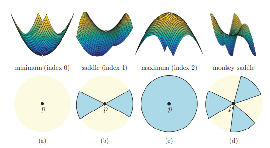
The value $D f(x)$ gives the rate of change of the value of $f$ at $x$. This can be visualized as the slope of the tangent line of the graph of $f$ at $(x, f(x))$. The critical points of $f$ are the set of points $x$ such that $D f(x)-0$. For a function defined on the real line, there are two types of critical points in the generic case: maxima and minima, as marked in Figure $1.8(b)$.
Now suppose we have a smooth function $f: \mathbb{R}^{d} \rightarrow \mathbb{R}$ defined on $\mathbb{R}^{d}$. Fix an arbitrary point $x \in \mathbb{R}^{d}$. As we move a little around $x$ within its local neighborhood, the rate of change of $f$ differs depending on which direction we move. This gives rise to the directional derivative $D_{v} f(x)$ at $x$ in direction (i.e., a unit vector) $v \in \mathbb{S}^{d-1}$, where $\mathbb{S}^{d-1}$ is the unit $(d-1)$-sphere, defined as
$$
D_{v} f(x)=\lim _{t \rightarrow 0} \frac{f(x+t \cdot v)-f(x)}{t}
$$
The gradient vector of $f$ at $x \in \mathbb{R}^{d}$ intuitively captures the direction of steepest increase of the function $f$. More precisely, we have the following.
Definition 1.25. (Gradient for functions on $\mathbb{R}^{d}$ ) Given a smooth function $f$ : $\mathbb{R}^{d} \rightarrow \mathbb{R}$, the gradient vector field $\nabla f: \mathbb{R}^{d} \rightarrow \mathbb{R}^{d}$ is defined as follows: for any $x \in \mathbb{R}^{d}$
$$
\nabla f(x)=\left[\frac{\partial f}{\partial x_{1}}(x), \frac{\partial f}{\partial x_{2}}(x), \ldots, \frac{\partial f}{\partial x_{d}}(x)\right]^{\mathrm{T}}
$$
where $\left(x_{1}, x_{2}, \ldots, x_{d}\right)$ represents an orthonormal coordinate system for $\mathbb{R}^{d}$. The vector $\nabla f(x) \in \mathbb{R}^{d}$ is called the gradient vector of $f$ at $x$. A point $x \in \mathbb{R}^{d}$ is a critical point if $\nabla f(x)=\left[\begin{array}{llll}0 & 0 & \ldots\end{array}\right]^{\mathrm{T}}$; otherwise, $x$ is regular.
数学代写|拓扑学代写Topology代考|Connection to Topology
We now characterize how critical points influence the topology of $M$ induced by the scalar function $f: M \rightarrow \mathbb{R}$.
Detinition 1.29. (Interval, sublevel, and superlevel sets) Given $f: M \rightarrow \mathbb{K}$ and $I \subseteq \mathbb{R}$, the interval levelset of $f$ with respect to $I$ is defined as
$$
M_{I}=f^{-1}(I)={x \in M \mid f(x) \in I}
$$
The case for $I=(-\infty, a]$ is also referred to as the sublevel set $M_{\leq a}:=$ $f^{-1}((-\infty, a])$ of $f$, while $M_{\geq a}:=f^{-1}([a, \infty))$ is called the superlevel set; and $f^{-1}(a)$ is called the levelset of $f$ at $a \in \mathbb{R} .$
Given $f: M \rightarrow \mathbb{R}$, imagine sweeping $M$ with increasing function values of $f$. It turns out that the topology of the sublevel sets can only change when we sweep through critical values of $f$. More precisely, we have the following classical result, where a diffeomorphism is a homeomorphism that is smooth in both directions.
Theorem 1.3. (Homotopy type of sublevel sets) Let $f: M \rightarrow \mathbb{R}$ be a smooth function defined on a manifold $M$. Given $a<b$, suppose the interval levelset $M_{[a, b]}=f^{-1}([a, b])$ is compact and contains no critical points of $f$. Then $M_{\leq a}$ is diffeomorphic to $M_{\leq b}$.
Furthermore, $M_{\leq a}$ is a deformation retract of $M_{\leq b}$, and the inclusion map $i: M_{\leq a} \hookrightarrow M_{\leq b}$ is a homotopy equivalence .
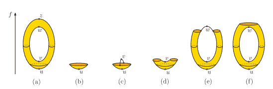
As an illustration, consider the example of height function $f: M \rightarrow \mathbb{R}$ defined on a vertical torus as shown in Figure $1.10(a)$. There are four critical points for the height function $f, u$ (minimum), $v, w$ (saddles), and $z$ (maximum). We have that $M_{\leq a}$ is: (i) empty for $af(z)$.
Theorem $1.3$ states that the homotopy type of the sublevel set remains the same until it passes a critical point. For Morse functions, we can also characterize the homotopy type of sublevel sets around critical points, captured by attaching $k$-cells.
数学代写|拓扑学代写Topology代考|Complexes and Homology Groups
This chapter introduces two very basic tools on which topological data analysis (TDA) is built. One is simplicial complexes and the other is homology groups. Data supplied as a discrete set of points do not have an interesting topology. Usually, we construct a scaffold on top of the data which is commonly taken as a simplicial complex. It consists of vertices at the data points, edges connecting them, and triangles, tetrahedra, and their higher-dimensional analogues that establish higher-order connectivity. Section $2.1$ formalizes this construction. There are different kinds of simplicial complexes. Some are easier to compute, but take more space. Others are more sparse, but take more time to compute. Section $2.2$ presents an important construction called the nerve and a complex called the Cech complex which is defined on this construction. This section also presents a commonly used complex in topological data analysis called the Vietoris-Rips complex that interleaves with the Cech complexes in terms of containment. In Section 2.3, we introduce some of the complexes which are sparser in size than the Vietoris-Rips or Čech complexes.
The second topic of this chapter, the homology groups of a simplicial complex, are the essential algebraic structures with which TDA analyzes data. Homology groups of a topological space capture the space of cycles up to those called boundaries that bound “higher-dimensional” subsets. For simplicity, we introduce the concept in the context of simplicial complexes instead of topological spaces. This is called simplicial homology. The essential entities for defining the homology groups are chains, cycles, and boundaries which we cover in Section 2.4. For simplicity and also for relevance in TDA, we define these structures under $\mathbb{Z}_{2}$-additions.
Section $2.5$ defines the simplicial homology group of a simplicial complex as the quotient space of the cycles with respect to the boundaries. Some of the concepts related to homology groups, such as induced homology under a map, singular homology groups for general topological spaces, relative homology groups of a complex with respect to a subcomplex, and the dual concept of homology groups, called cohomology groups are also introduced in this section.
拓扑学代考
数学代写|拓扑学代写Topology代考|Gradients and Critical Points
在下文中,为简单起见,我们假设我们认为平滑 ( $C^{\infty}$ – 连续) 函数和嵌入的平滑流形 $\mathbb{R}^{d}$ ,即使我们通常只需要函 数 (分别是流形) 是 $C^{2}$ 连续 (分别 $C^{2}$-光滑的)。
为了直观起见,让我们从定义在实线上的平滑标量函数开始, $f: \mathbb{R} \rightarrow \mathbb{R}$; 这种函数的图形如图所示 $1.8(\mathrm{~b})$. 回想 一下函数在一点的导数 $x \in \mathbb{R}$ 定义为
$$
D f(x)=\frac{d}{d x} f(x)=\lim {t \rightarrow 0} \frac{f(x+t)-f(x)}{t} $$ 价值 $D f(x)$ 给出值的变化率 $f$ 在 $x$. 这可以可视化为图形的切线的斜率 $f$ 在 $(x, f(x))$. 的关键点 $f$ 是点的集合 $x$ 这样 $D f(x)-0$. 对于定义在实线上的函数,一般情况下有两种临界点:极大值和极小值,如图所示 $1.8(b)$. 现在假设我们有一个平滑函数 $f: \mathbb{R}^{d} \rightarrow \mathbb{R}$ 定义于 $\mathbb{R}^{d}$. 修复任意点 $x \in \mathbb{R}^{d}$. 当我们稍微移动一下 $x$ 在其当地社区 内,变化率 $f$ 根据我们移动的方向而有所不同。这产生了方向导数 $D{v} f(x)$ 在 $x$ 在方向 (即,单位向量) $v \in \mathbb{S}^{d-1}$ ,在哪里S ${ }^{d-1}$ 是单位 $(d-1)$-sphere,定义为
$$
D_{v} f(x)=\lim {t \rightarrow 0} \frac{f(x+t \cdot v)-f(x)}{t} $$ 的梯度向量 $f$ 在 $x \in \mathbb{R}^{d}$ 直观地捕捉到函数增长最陡的方向 $f$. 更准确地说,我们有以下内容。 定义 1.25。(函数的梯度 $\mathbb{R}^{d}$ ) 给定一个平滑函数 $f: \mathbb{R}^{d} \rightarrow \mathbb{R}$, 梯度向量场 $\nabla f: \mathbb{R}^{d} \rightarrow \mathbb{R}^{d}$ 定义如下: 对于任何 $x \in \mathbb{R}^{d}$ $$ \nabla f(x)=\left[\frac{\partial f}{\partial x{1}}(x), \frac{\partial f}{\partial x_{2}}(x), \ldots, \frac{\partial f}{\partial x_{d}}(x)\right]^{\mathrm{T}}
$$
在哪里 $\left(x_{1}, x_{2}, \ldots, x_{d}\right)$ 表示正交坐标系 $\mathbb{R}^{d}$. 向量 $\nabla f(x) \in \mathbb{R}^{d}$ 称为梯度向量 $f$ 在 $x$. 一点 $x \in \mathbb{R}^{d}$ 是一个临界 点,如果 $\nabla f(x)=\left[\begin{array}{lll}0 & 0 & \ldots\end{array}\right]^{\mathrm{T}}$; 否则, $x$ 是规律的。
数学代写|拓扑学代写Topology代考|Connection to Topology
我们现在描述临界点如何影响拓扑 $M$ 由标量函数诱导 $f: M \rightarrow \mathbb{R}$.
定义 1.29。(区间、子级和超级集) 给定 $f: M \rightarrow \mathbb{K}$ 和 $I \subseteq \mathbb{R}$ ,区间水平集 $f$ 关于 $I$ 定义为
$$
M_{I}=f^{-1}(I)=x \in M \mid f(x) \in I
$$
案例为 $I=(-\infty, a]$ 也称为子水平集 $M_{\leq a}:=f^{-1}((-\infty, a])$ 的 $f$ ,尽管 $M_{\geq a}:=f^{-1}([a, \infty))$ 称为超水平 集;和 $f^{-1}(a)$ 称为水平集 $f$ 在 $a \in \mathbb{R}$.
给定 $f: M \rightarrow \mathbb{R}$ ,想象一下 $M$ 随着函数值的增加 $f$. 事实证明,子水平集的拓扑只有在我们扫描 $f$. 更准确地说, 我们有以下经典结果,其中微分同䏣是在两个方向上都光滑的同胚。
定理 1.3。 (子水平集的同伦类型) 让 $f: M \rightarrow \mathbb{R}$ 是定义在流形上的平滑函数 $M$. 给定 $a<b$ ,假设区间水平集 $M_{[a, b]}=f^{-1}([a, b])$ 是紧凑的,不包含关键点 $f$. 然后 $M_{\leq a}$ 微分同胚于 $M_{\leq b}$.
此外, $M_{\leq a}$ 是变形缩回 $M_{\leq b}$ ,和包含图 $i: M_{\leq a} \hookrightarrow M_{\leq b}$ 是同伦等价的。
作为说明,考虑高度函数的示例 $f: M \rightarrow \mathbb{R}$ 定义在如图所示的垂直圆环上 $1.10(a)$. 高度函数有四个临界点 $f, u$ (最低限度), $v, w$ (马鞍),和 $z$ (最大) 。我们有那个 $M_{\leq a}$ 是: (i) 为空 $a f(z)$.
定理1.3表示子水平集的同伦类型保持不变,直到它通过一个临界点。对于 Morse 函数,我们还可以表征围绕临界 点的子水平集的同伦类型,通过附加 $k$-细胞。
数学代写|拓扑学代写Topology代考|Complexes and Homology Groups
本章介绍了构建拓扑数据分析 (TDA) 的两个非常基本的工具。一种是单纯复形,另一种是同调群。作为离散点集提供的数据没有有趣的拓扑。通常,我们在通常被视为单纯复形的数据之上构建一个脚手架。它由数据点处的顶点、连接它们的边、三角形、四面体及其建立高阶连通性的高维类似物组成。部分2.1形式化这个结构。有不同种类的单纯复形。有些更容易计算,但占用更多空间。其他更稀疏,但需要更多时间来计算。部分2.2提出了一种称为神经的重要结构和一种称为 Cech 复合体的复合体,该复合体是在该结构上定义的。本节还介绍了拓扑数据分析中常用的复合体,称为 Vietoris-Rips 复合体,它在包容性方面与 Cech 复合体交错。在第 2.3 节中,我们介绍了一些尺寸比 Vietoris-Rips 或 Čech 复合体更稀疏的复合体。
本章的第二个主题,单纯复形的同调群,是 TDA 分析数据的基本代数结构。拓扑空间的同调群捕获循环空间,直到那些称为边界的边界,这些边界绑定了“高维”子集。为简单起见,我们在单纯复形而不是拓扑空间的背景下引入了这个概念。这称为单纯同调。定义同调群的基本实体是我们在 2.4 节中介绍的链、循环和边界。为了简单起见,也为了与 TDA 相关,我们将这些结构定义为从2-添加。
部分2.5将单纯复形的单纯同调群定义为环相对于边界的商空间。一些与同调群相关的概念,例如映射下的诱导同调、一般拓扑空间的奇异同调群、复形相对于子复形的相对同调群,以及同调群的对偶概念,称为上同调群。本节介绍。

统计代写请认准statistics-lab™. statistics-lab™为您的留学生涯保驾护航。
金融工程代写
金融工程是使用数学技术来解决金融问题。金融工程使用计算机科学、统计学、经济学和应用数学领域的工具和知识来解决当前的金融问题,以及设计新的和创新的金融产品。
非参数统计代写
非参数统计指的是一种统计方法,其中不假设数据来自于由少数参数决定的规定模型;这种模型的例子包括正态分布模型和线性回归模型。
广义线性模型代考
广义线性模型(GLM)归属统计学领域,是一种应用灵活的线性回归模型。该模型允许因变量的偏差分布有除了正态分布之外的其它分布。
术语 广义线性模型(GLM)通常是指给定连续和/或分类预测因素的连续响应变量的常规线性回归模型。它包括多元线性回归,以及方差分析和方差分析(仅含固定效应)。
有限元方法代写
有限元方法(FEM)是一种流行的方法,用于数值解决工程和数学建模中出现的微分方程。典型的问题领域包括结构分析、传热、流体流动、质量运输和电磁势等传统领域。
有限元是一种通用的数值方法,用于解决两个或三个空间变量的偏微分方程(即一些边界值问题)。为了解决一个问题,有限元将一个大系统细分为更小、更简单的部分,称为有限元。这是通过在空间维度上的特定空间离散化来实现的,它是通过构建对象的网格来实现的:用于求解的数值域,它有有限数量的点。边界值问题的有限元方法表述最终导致一个代数方程组。该方法在域上对未知函数进行逼近。[1] 然后将模拟这些有限元的简单方程组合成一个更大的方程系统,以模拟整个问题。然后,有限元通过变化微积分使相关的误差函数最小化来逼近一个解决方案。
tatistics-lab作为专业的留学生服务机构,多年来已为美国、英国、加拿大、澳洲等留学热门地的学生提供专业的学术服务,包括但不限于Essay代写,Assignment代写,Dissertation代写,Report代写,小组作业代写,Proposal代写,Paper代写,Presentation代写,计算机作业代写,论文修改和润色,网课代做,exam代考等等。写作范围涵盖高中,本科,研究生等海外留学全阶段,辐射金融,经济学,会计学,审计学,管理学等全球99%专业科目。写作团队既有专业英语母语作者,也有海外名校硕博留学生,每位写作老师都拥有过硬的语言能力,专业的学科背景和学术写作经验。我们承诺100%原创,100%专业,100%准时,100%满意。
随机分析代写
随机微积分是数学的一个分支,对随机过程进行操作。它允许为随机过程的积分定义一个关于随机过程的一致的积分理论。这个领域是由日本数学家伊藤清在第二次世界大战期间创建并开始的。
时间序列分析代写
随机过程,是依赖于参数的一组随机变量的全体,参数通常是时间。 随机变量是随机现象的数量表现,其时间序列是一组按照时间发生先后顺序进行排列的数据点序列。通常一组时间序列的时间间隔为一恒定值(如1秒,5分钟,12小时,7天,1年),因此时间序列可以作为离散时间数据进行分析处理。研究时间序列数据的意义在于现实中,往往需要研究某个事物其随时间发展变化的规律。这就需要通过研究该事物过去发展的历史记录,以得到其自身发展的规律。
回归分析代写
多元回归分析渐进(Multiple Regression Analysis Asymptotics)属于计量经济学领域,主要是一种数学上的统计分析方法,可以分析复杂情况下各影响因素的数学关系,在自然科学、社会和经济学等多个领域内应用广泛。
MATLAB代写
MATLAB 是一种用于技术计算的高性能语言。它将计算、可视化和编程集成在一个易于使用的环境中,其中问题和解决方案以熟悉的数学符号表示。典型用途包括:数学和计算算法开发建模、仿真和原型制作数据分析、探索和可视化科学和工程图形应用程序开发,包括图形用户界面构建MATLAB 是一个交互式系统,其基本数据元素是一个不需要维度的数组。这使您可以解决许多技术计算问题,尤其是那些具有矩阵和向量公式的问题,而只需用 C 或 Fortran 等标量非交互式语言编写程序所需的时间的一小部分。MATLAB 名称代表矩阵实验室。MATLAB 最初的编写目的是提供对由 LINPACK 和 EISPACK 项目开发的矩阵软件的轻松访问,这两个项目共同代表了矩阵计算软件的最新技术。MATLAB 经过多年的发展,得到了许多用户的投入。在大学环境中,它是数学、工程和科学入门和高级课程的标准教学工具。在工业领域,MATLAB 是高效研究、开发和分析的首选工具。MATLAB 具有一系列称为工具箱的特定于应用程序的解决方案。对于大多数 MATLAB 用户来说非常重要,工具箱允许您学习和应用专业技术。工具箱是 MATLAB 函数(M 文件)的综合集合,可扩展 MATLAB 环境以解决特定类别的问题。可用工具箱的领域包括信号处理、控制系统、神经网络、模糊逻辑、小波、仿真等。