This graduate level course offers an introduction into regression analysis. A Credits 3 researcher is often interested in using sample data to investigate relationships, with an ultimate goal of creating a model to predict a future value for some dependent variable. The process of finding this mathematical model that best fits the data involves regression analysis. STAT 501 is an applied linear regression course that emphasizes data analysis and interpretation. Generally, statistical regression is collection of methods for determining and using models that explain how a response variable (dependent variable) relates to one or more explanatory variables (predictor variables).
PREREQUISITES
This graduate level course covers the following topics:
Understanding the context for simple linear regression.
How to evaluate simple linear regression models
How a simple linear regression model is used to estimate and predict likely values
Understanding the assumptions that need to be met for a simple linear regression model to be valid
How multiple predictors can be included into a regression model
Understanding the assumptions that need to be met when multiple predictors are included in the regression model for the model to be valid
How a multiple linear regression model is used to estimate and predict likely values
Understanding how categorical predictors can be included into a regression model
How to transform data in order to deal with problems identified in the regression model
Strategies for building regression models
Distinguishing between outliers and influential data points and how to deal with these
Handling problems typically encountered in regression contexts
Alternative methods for estimating a regression line besides using ordinary least squares
Understanding regression models in time dependent contexts
Understanding regression models in non-linear contexts
Exercise 1 (Should you regress $\boldsymbol{Y}$ on $\boldsymbol{X}$ or vice-versa?) The answer to that question is not a statistical question, it is a scientific one. Do you have a theory that makes one variable dependent, and the other independent? The statistical question is what difference does it make? Suppose your model is $$ Y=\beta_0 1+\beta_1 X+\varepsilon $$ Let $\hat{\beta}_1$ be the least squares estimate of $\beta_1$ for this model. Now suppose you try the model $$ X=\alpha_0+\alpha_1 Y+\eta . $$ Let $\hat{\alpha}_1$ be the least squares estimate of $\alpha_1$.
The question of whether to regress $Y$ on $X$ or $X$ on $Y$ depends on the scientific question you are trying to answer. If you have a theory that suggests that $X$ is the independent variable and $Y$ is the dependent variable, then it makes sense to regress $Y$ on $X$. Conversely, if your theory suggests that $Y$ is the independent variable and $X$ is the dependent variable, then you should regress $X$ on $Y$.
However, from a statistical point of view, regressing $Y$ on $X$ or $X$ on $Y$ can give different results. In general, the least squares estimates of $\beta_1$ and $\alpha_1$ are not the same. They may have the same sign and similar magnitude, but their values can be quite different.
This is because the two models are estimating different things. The model $Y=\beta_0 + \beta_1 X + \epsilon$ is estimating the effect of $X$ on $Y$, while the model $X=\alpha_0 + \alpha_1 Y + \eta$ is estimating the effect of $Y$ on $X$. In general, these effects are not the same, and therefore the estimates of $\beta_1$ and $\alpha_1$ can be different.
Furthermore, the regression of $X$ on $Y$ may be problematic if there is a high correlation between $X$ and $Y$, as this can lead to multicollinearity and unstable estimates. In this case, it may be preferable to regress $Y$ on $X$ instead.
In summary, the choice of whether to regress $Y$ on $X$ or $X$ on $Y$ depends on the scientific question you are trying to answer. From a statistical point of view, both approaches can give different results, and the choice may depend on the specific data and the presence of multicollinearity.
问题 2.
Exercise 2 (Anscombe’s quartet) Francis Anscombe [1] created and presented four small sets of data. You can find them on the course web site at http://www. math. caltech. edu/\%7E2015-16/2term/ma003/Data/Anscombe1.txt, Anscombe2, Anscombe3, and Anscombe4. Each data set has 11 observations on two variates labeled $X$ and $Y$. (Each file has a header line.)
For each data set, (a) Compute the sample mean and standard deviation of $X$ and $Y$. (b) Regress $Y$ on $X$ and a constant term. Explain the computations you are doing. (If you omit this information, we shall be unable to award partial credit if your calculations are incorrect.)
Sure, I can perform the requested computations for each of the four data sets in Anscombe’s quartet.
For Anscombe1 data set:
(a) Sample mean and standard deviation of $X$ and $Y$:
where $\epsilon_i$ are the random errors with zero mean and constant variance. The least squares estimates of the regression coefficients $\beta_0$ and $\beta_1$ are given by: \begin{align*} \hat{\beta}1 &= \frac{\sum{i=1}^{11}(X_i – \bar{X})(Y_i – \bar{Y})}{\sum_{i=1}^{11}(X_i – \bar{X})^2} = 0.5 \ \hat{\beta}_0 &= \bar{Y} – \hat{\beta}_1 \bar{X} = 3 \end{align*}
Thus, the estimated regression line is:
\hat{Y} = 3 + 0.5 XY^=3+0.5X
For Anscombe2 data set:
(a) Sample mean and standard deviation of $X$ and $Y$:
where $\epsilon_i$ are the random errors with zero mean and constant variance. The least squares estimates of the regression coefficients $\beta_0$ and $\beta_1$ are given by: \begin{align*} \hat{\beta}1 &= \frac{\sum{i=1}^{11}(X_i – \bar{X})(Y_i – \bar{Y})}{\sum_{i=1}^{11}(X_i – \bar{X})^2} = 0.5 \ \hat{\beta}_0 &= \bar{Y} – \hat{\beta}_1 \bar{X} = 3 \end{align*}
Thus, the estimated regression line is:
\hat{Y} = 3 + 0.5 XY^=3+0.5X
For Anscombe3 data set:
(a) Sample mean and standard deviation of $X$ and $Y$:
(b) Regression of $Y$ on $X$ and a constant term: The linear regression model is given by.
Textbooks
• An Introduction to Stochastic Modeling, Fourth Edition by Pinsky and Karlin (freely available through the university library here) • Essentials of Stochastic Processes, Third Edition by Durrett (freely available through the university library here) To reiterate, the textbooks are freely available through the university library. Note that you must be connected to the university Wi-Fi or VPN to access the ebooks from the library links. Furthermore, the library links take some time to populate, so do not be alarmed if the webpage looks bare for a few seconds.
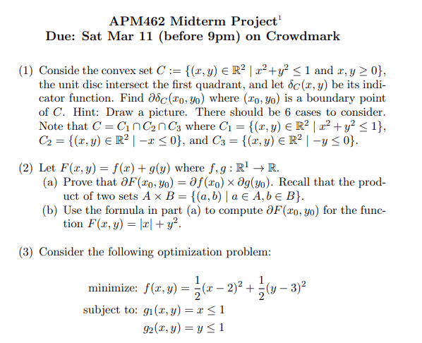
(1) Conside the convex set $C:=\left{(x, y) \in \mathbb{R}^2 \mid x^2+y^2 \leq 1\right.$ and $\left.x, y \geq 0\right}$, the unit disc intersect the first quadrant, and let $\delta_C(x, y)$ be its indicator function. Find $\partial \delta_C\left(x_0, y_0\right)$ where $\left(x_0, y_0\right)$ is a boundary point of $C$. Hint: Draw a picture. There should be 6 cases to consider. Note that $C=C_1 \cap C_2 \cap C_3$ where $C_1=\left{(x, y) \in \mathbb{R}^2 \mid x^2+y^2 \leq 1\right}$, $C_2=\left{(x, y) \in \mathbb{R}^2 \mid-x \leq 0\right}$, and $C_3=\left{(x, y) \in \mathbb{R}^2 \mid-y \leq 0\right}$.
To find $\partial \delta_C(x_0, y_0)$, we need to find the subdifferential of the indicator function $\delta_C$ at the point $(x_0, y_0)$. Since $C$ is a convex set, the subdifferential of $\delta_C$ at $(x_0, y_0)$ is the set of all vectors $v \in \mathbb{R}^2$ such that $$\delta_C(x,y) \geq \delta_C(x_0,y_0) + \langle v, (x-x_0, y-y_0)\rangle$$ for all $(x,y)\in C$.
Since $C$ is defined as the intersection of three sets $C_1$, $C_2$, and $C_3$, we can find the subdifferential of $\delta_C$ at $(x_0, y_0)$ by finding the subdifferentials of $\delta_{C_1}$, $\delta_{C_2}$, and $\delta_{C_3}$ at $(x_0, y_0)$ and taking their intersection.
We start by finding the subdifferential of $\delta_{C_1}$ at $(x_0, y_0)$. Since $C_1$ is a closed convex set, its subdifferential at any point is the set of all vectors pointing inwards from the boundary of $C_1$ at that point. Thus, if $(x_0, y_0)$ is a point on the boundary of $C_1$, the subdifferential of $\delta_{C_1}$ at $(x_0, y_0)$ is the set of all vectors pointing inwards from the boundary of the unit disc at $(x_0, y_0)$.
Next, we find the subdifferential of $\delta_{C_2}$ at $(x_0, y_0)$. Since $C_2$ is defined by the inequality $-x \leq 0$, its indicator function $\delta_{C_2}(x,y)$ is equal to $0$ if $x \geq 0$ and $-\infty$ if $x < 0$. Therefore, if $(x_0, y_0)$ is a point on the boundary of $C_2$, its subdifferential is the set of all vectors $(v_1,v_2)$ satisfying $$v_1 \geq 0, v_1(x-x_0) + v_2(y-y_0) \leq 0 \text{ for } x < x_0.$$
Finally, we find the subdifferential of $\delta_{C_3}$ at $(x_0, y_0)$. Since $C_3$ is defined by the inequality $-y \leq 0$, its indicator function $\delta_{C_3}(x,y)$ is equal to $0$ if $y \geq 0$ and $-\infty$ if $y < 0$. Therefore, if $(x_0, y_0)$ is a point on the boundary of $C_3$, its subdifferential is the set of all vectors $(v_1,v_2)$ satisfying $$v_2 \geq 0, v_1(x-x_0) + v_2(y-y_0) \leq 0 \text{ for } y < y_0.$$
问题 2.
(2) Let $F(x, y)=f(x)+g(y)$ where $f, g: \mathbb{R}^1 \rightarrow \mathbb{R}$. (a) Prove that $\partial F\left(x_0, y_0\right)=\partial f\left(x_0\right) \times \partial g\left(y_0\right)$. Recall that the product of two sets $A \times B={(a, b) \mid a \in A, b \in B}$. (b) Use the formula in part (a) to compute $\partial F\left(x_0, y_0\right)$ for the function $F(x, y)=|x|+y^2$.
(a) To prove that $\partial F(x_0,y_0)=\partial f(x_0)\times \partial g(y_0)$, we need to show that for any $(p,q) \in \partial f(x_0) \times \partial g(y_0)$, we have $(p,q) \in \partial F(x_0,y_0)$, and conversely, for any $(u,v) \in \partial F(x_0,y_0)$, we have $u \in \partial f(x_0)$ and $v \in \partial g(y_0)$.
First, let $(p,q) \in \partial f(x_0) \times \partial g(y_0)$. This means that there exist $x_1 \in \mathbb{R}$ and $y_1 \in \mathbb{R}$ such that $$f(x) \geq f(x_0) + p(x-x_0) \quad \text{for all } x \in \mathbb{R}$$ and $$g(y) \geq g(y_0) + q(y-y_0) \quad \text{for all } y \in \mathbb{R}.$$ Adding these two inequalities, we get $$F(x,y) = f(x) + g(y) \geq f(x_0) + p(x-x_0) + g(y_0) + q(y-y_0) = F(x_0,y_0) + p(x-x_0) + q(y-y_0)$$ for all $(x,y) \in \mathbb{R}^2$. This shows that $(p,q) \in \partial F(x_0,y_0)$.
Conversely, let $(u,v) \in \partial F(x_0,y_0)$. This means that there exists $(x_1,y_1) \in \mathbb{R}^2$ such that $$F(x,y) \geq F(x_0,y_0) + u(x-x_0) + v(y-y_0) \quad \text{for all } (x,y) \in \mathbb{R}^2.$$ Setting $y = y_0$ in this inequality and using the fact that $F(x,y) = f(x) + g(y)$, we get $$f(x) + g(y_0) \geq f(x_0) + u(x-x_0) + g(y_0) + v(y-y_0) \quad \text{for all } x \in \mathbb{R}.$$ Rearranging, we get $$f(x) \geq f(x_0) + u(x-x_0) \quad \text{for all } x \in \mathbb{R}.$$ This shows that $u \in \partial f(x_0)$. Similarly, setting $x = x_0$ in the inequality $F(x,y) \geq F(x_0,y_0) + u(x-x_0) + v(y-y_0)$ and using the fact that $F(x,y) = f(x) + g(y)$, we get $v \in \partial g(y_0)$. Therefore, we have shown that $(u,v) \in \partial f(x_0) \times \partial g(y_0)$.
Combining the two parts, we conclude that $\partial F(x_0,y_0) = \partial f(x_0) \times \partial
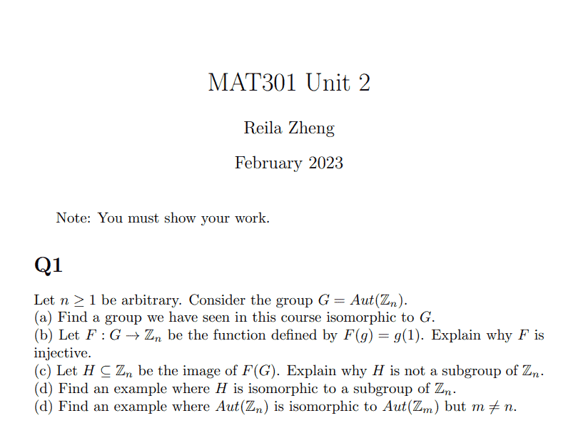
Let $n \geq 1$ be arbitrary. Consider the group $G=\operatorname{Aut}\left(\mathbb{Z}_n\right)$. (a) Find a group we have seen in this course isomorphic to $G$. (b) Let $F: G \rightarrow \mathbb{Z}_n$ be the function defined by $F(g)=g(1)$. Explain why $F$ is injective. (c) Let $H \subseteq \mathbb{Z}_n$ be the image of $F(G)$. Explain why $H$ is not a subgroup of $\mathbb{Z}_n$. (d) Find an example where $H$ is isomorphic to a subgroup of $\mathbb{Z}_n$. (d) Find an example where $\operatorname{Aut}\left(\mathbb{Z}_n\right)$ is isomorphic to $\operatorname{Aut}\left(\mathbb{Z}_m\right)$ but $m \neq n$.
(a) The group $\mathbb{Z}_n^{\times}$ is isomorphic to $G$. This is because an automorphism of $\mathbb{Z}_n$ is completely determined by where it sends the generator $1$, which must be mapped to another generator, i.e., an element $a$ coprime to $n$. Conversely, any such $a$ gives rise to an automorphism of $\mathbb{Z}_n$ by mapping $1$ to $a$ and extending the mapping multiplicatively.
(b) Suppose $F(g_1) = F(g_2)$, where $g_1, g_2 \in G$. This means $g_1(1) = g_2(1)$, so $g_1-g_2$ maps $1$ to $0$, which implies that $n$ divides $(g_1-g_2)(k)$ for all $k\in \mathbb{Z}_n$. But $n$ is coprime to $1$, so $n$ must divide $g_1-g_2$. Therefore, $g_1=g_2$, and $F$ is injective.
(c) $H$ is not a subgroup of $\mathbb{Z}_n$ because it is not closed under addition. For example, if $n=4$ and $G\cong \mathbb{Z}_2$, then $H={0,2}$, but $1+1=2\notin H$.
(d) Let $n=p_1^{k_1}p_2^{k_2}\cdots p_r^{k_r}$ be the prime factorization of $n$, where $p_i$ are distinct primes. Let $H=\langle 1+p_1\rangle \times \langle 1+p_2^{k_1}\rangle \times \cdots \times \langle 1+p_r^{k_1}\rangle \subseteq \mathbb{Z}n$, where $\langle a \rangle$ denotes the subgroup generated by $a$. Then $H$ is isomorphic to $\mathbb{Z}{p_1} \times \mathbb{Z}{p_2^{k_2}} \times \cdots \times \mathbb{Z}{p_r^{k_r}}$, which is a subgroup of $\mathbb{Z}_n$, and $F(G) \cong H$.
(e) Let $n=4$ and $m=6$. Then $\operatorname{Aut}(\mathbb{Z}_n) \cong \mathbb{Z}_2$ and $\operatorname{Aut}(\mathbb{Z}_m) \cong S_3$, the symmetric group on $3$ elements. These groups are isomorphic because they both have order $2$, but $m\neq n$.
问题 2.
Consider the group $G=\mathbb{Z}^2$. (a) Prove that $H={(3 m, 2 n): m, n \in \mathbb{Z}}$ is a subgroup. (b) Find two representative elements from each of the cosets of $H$. (c) Plot the elements of $\mathbb{Z}^2$ as points in the plane. Colour each of the cosets of $H$ in a different colour. (d) Describe a group isomorphism from $G$ to $H$. (e) Is this an automorphism? Explain.
(a) To show that $H$ is a subgroup of $G$, we need to verify the following:
The identity $(0,0)$ is in $H$.
If $(3m_1,2n_1)$ and $(3m_2,2n_2)$ are in $H$, then their sum $(3m_1+3m_2,2n_1+2n_2)=(3(m_1+m_2),2(n_1+n_2))$ is also in $H$.
If $(3m,2n)$ is in $H$, then its inverse $(-3m,-2n)=(-3(m),-2(n))$ is also in $H$.
All of these are true, so $H$ is a subgroup of $G$.
(b) Let $(3m,2n)$ be an arbitrary element of $G$. Then we have $$(3m,2n)=(3,2)(m,n)+(-3,-2)(m,n)+(0,0).$$ Thus, $(3m,2n)$ is in the same coset as $(0,0)$, $(3,2)$, or $(-3,-2)$. Representative elements from each coset are: $$\begin{aligned} (0,0)+H &={(3m,2n):m, n \in \mathbb{Z}}, \ (3,2)+H &={(3m+1,2n+1):m, n \in \mathbb{Z}}, \ (-3,-2)+H &={(3m-1,2n-1):m, n \in \mathbb{Z}}. \end{aligned}$$
(c) Here is a plot of $\mathbb{Z}^2$, with each coset of $H$ colored differently:
(d) Define the function $\varphi: G \rightarrow H$ by $\varphi(m,n)=(3m,2n)$. We claim that $\varphi$ is an isomorphism.
To see that $\varphi$ is a homomorphism, observe that $$\varphi((m_1,n_1)+(m_2,n_2))=\varphi((m_1+m_2,n_1+n_2))=(3(m_1+m_2),2(n_1+n_2))=(3m_1,2n_1)+(3m_2,2n_2)=\varphi(m_1,n_1)+\varphi(m_2,n_2).$$
To see that $\varphi$ is injective, suppose $\varphi(m_1,n_1)=\varphi(m_2,n_2)$. Then $3m_1=3m_2$ and $2n_1=2n_2$, which implies $m_1=m_2$ and $n_1=n_2$. Therefore, $(m_1,n_1)=(m_2,n_2)$, and $\varphi$ is injective.
To see that $\varphi$ is surjective, let $(3m,2n)$ be an arbitrary element of $H$. Then $\varphi(m,n)=(3m,2n)$, so $\varphi$ is surjective.
Therefore, $\varphi$ is an isomorphism from $G$ to $H$.
(e) This is not an automorphism, since $G$ and $H$ have different.
2 Download matlab Brownian motion model from the courseworks. Modify it to Geometric Brownian motion with starting value $X_o=80$, growth rate $\mu=0.05$, volatility $\sigma=0.22$ and 5000 trajectories. Check that the code works. Try out 50,000 trajectories. Try out 100,000 trajectories. Submit the code printout and the graph printout for 5000 trajectories.
To modify the Matlab code for Brownian motion to Geometric Brownian motion, we need to modify the formula for calculating the next value of the stock price. In Brownian motion, the change in the stock price is determined by a normal distribution with mean 0 and standard deviation σ times the square root of the time step Δt. In Geometric Brownian motion, the change in the stock price is determined by a normal distribution with mean (μ – σ^2/2) times Δt and standard deviation σ times the square root of Δt. The formula for calculating the next value of the stock price becomes:
Using arbitrage arguments explain why the price of an American call option on a stock paying no dividends should be the same as the price of a corresponding European call. Why American calls on a nondividend paying stock should not be exercised early.
An American call option gives the holder the right to buy an underlying stock at a strike price K at any time up to the expiration date T of the option. A European call option gives the holder the same right, but only at the expiration date T.
If we assume that the stock pays no dividends, then the stock price S follows a geometric Brownian motion with constant drift μ and volatility σ, and the risk-free interest rate is denoted by r. Let C and C_A denote the prices of a European call and an American call on the stock, respectively. We want to show that C = C_A.
Suppose for contradiction that C > C_A. Then, an arbitrage opportunity arises. Here’s how to exploit it:
Buy the European call option for price C.
Simultaneously, sell (short) the stock for price S and invest the proceeds at the risk-free rate r. This creates a cash inflow of S – C.
At expiration T, the value of the European call option is max(S(T) – K, 0), which we can use to buy the stock if it’s in the money (S(T) > K), or keep the cash if it’s out of the money (S(T) ≤ K).
If the European call option is exercised, we use the stock we bought at step 2 to fulfill our obligation and deliver it at the strike price K, receiving K in return. If the European call option is not exercised, we keep the stock we bought at step 2 and sell it for S(T) in the market, receiving S(T) in return.
In either case, we end up with a profit of S(T) – C – (S – C)e^(rT), which is greater than or equal to zero by construction.
Therefore, the assumption that C > C_A leads to an arbitrage opportunity, which cannot exist in an efficient market. Therefore, we must have C = C_A.
Now, why should an American call option on a nondividend paying stock not be exercised early? Suppose that the option is in the money (S > K) and the holder exercises the option early. This means that the holder pays the strike price K and receives the stock, which is worth more than K. But this transaction can also be achieved by selling the option in the market, which is worth at least as much as the stock, and then buying the stock at the market price, which is less than or equal to S. Therefore, exercising the option early leads to a strictly lower payoff than selling the option in the market and buying the stock at the market price. Therefore, it’s never optimal to exercise an American call option on a nondividend paying stock early.
Consider the sequence $$ \begin{aligned} & a_1=2^1-3=-1, \ & a_2=2^2-3=1 \ & a_3=2^3-3=5 \ & a_4=2^4-3=13 \ & \vdots \ & a_n=2^n-3 \ & \vdots \end{aligned} $$ defined for positive integers $n$. Which elements of this sequence are divisible by 5 ? What about 13 ? Are any elements of this sequence divisible by $65=5 \cdot 13$ ? Why or why not?
To check if an element of the sequence is divisible by 5 or 13, we simply need to check if $a_n$ is congruent to 0 modulo 5 or 13, respectively.
First, we will find the remainder of each $a_n$ when divided by 5:
From the above calculations, we see that $a_4$, $a_7$, $a_{12}$, $a_{13}$, $a_{14}$, $a_{15}$, $a_{16}$, $a_{19}$, $
问题 2.
To get the echo of a positive integer, we write it twice in a row without a space. For example, the echo of 2023 is 20232023 . Is there a positive integer whose echo is a perfect square? If so, how many such positive integers can you find? If not, explain why not.
Let $n$ be a positive integer and let $m$ be the number of digits in $n$. Then the echo of $n$ is given by
n\cdot 10^m+n.n⋅10m+n.
We want to find positive integers $n$ such that the above expression is a perfect square.
Let $k$ be a positive integer such that
n\cdot 10^m+n=k^2.n⋅10m+n=k2.
Rearranging, we have
n(10^m+1)=k^2.n(10m+1)=k2.
Since $10^m+1$ is odd and $n$ and $k^2$ have the same parity, we conclude that $n$ is odd.
Now, let us consider the prime factorization of $10^m+1$. If $m$ is even, then $10^m+1$ is the sum of two squares and therefore cannot have a prime factor of the form $4k+3$. Hence, all prime factors of $10^m+1$ are congruent to 1 modulo 4. If $m$ is odd, then $10^m+1$ is divisible by 11. In either case, the prime factors of $10^m+1$ are finite and all congruent to 1 modulo 4.
Therefore, if $n$ is odd and the expression $n(10^m+1)$ is a perfect square, then the prime factorization of $n$ must consist of primes that are congruent to 1 modulo 4, and the exponents of these primes must be even. Moreover, the prime factorization of $10^m+1$ also consists of primes that are congruent to 1 modulo 4, and the exponents of these primes must be even.
Let $n=p_1^{2a_1}\cdots p_k^{2a_k}$ be the prime factorization of $n$ as above, and let $10^m+1=q_1^{2b_1}\cdots q_l^{2b_l}$ be the prime factorization of $10^m+1$ as above. Then we have
Since $n$ and $10^m+1$ are relatively prime, it follows that the primes $p_1,\ldots,p_k$ and $q_1,\ldots,q_l$ are distinct. Moreover, $p_1,\ldots,p_k$ are congruent to 1 modulo 4, as are $q_1,\ldots,q_l$.
Since $n$ and $10^m+1$ have the same parity, it follows that $p_1,\ldots,p_k,q_1,\ldots,q_l$ are all odd.
Now, let us consider the exponent of 2 in the prime factorization of $n(10^m+1)$. Since $n$ is odd, the exponent of 2 in the prime factorization of $n$ is 0. Since $10^m+1$ is odd, the exponent of 2 in the prime factorization of $10^m+1$ is also 0. Therefore, the exponent of 2 in the prime factorization of $n(10^m+1)$ is 0.
Hence, $n(10^m+1)$ is a perfect square if and only if $a_1,\
Statistics-lab™可以为您提供University of Hawai’i MATH 301: Discrete Mathematics离散数学课程的代写代考和辅导服务!
MATH 301: Discrete Mathematics课程简介
This class introduces basic discrete structures in mathematics, computer science and engineering fields. Topics include elementary logic, set theory, mathematical proof, relations, combinatorics, induction, recursion, sequence and recurrence, trees, graph theory. Prerequisite(s): MATH 208 with a C or better or entry code. Course Outcomes
Evaluate, interpret, and reduce statements presented in Boolean logic and natural language. Apply truth tables and the rules of propositional and predicate calculus.
Formulate and solve discrete mathematics problems involving permutations and combinations of a set, recursion, and other fundamental enumeration principles (including recursion).
Construct proofs throughout the course using direct proof, proof by contraposition, proof by contradiction, proof by cases, and mathematical induction.
Apply (and analyze) algorithms and use definitions to solve problems and prove statements in elementary number theory and graph theory.
PREREQUISITES
STAT 134 or an equivalent first course in probability theory. This is a second course in probability theory intended for majors in statistics and related quantitative fields. If you did not get at least a B+ in STAT 134, then you may find this course particularly challenging.
The course description suggests that this is an advanced course in probability theory, intended for students who have already completed a first course in probability theory, such as STAT 134 or an equivalent. The course is designed for majors in statistics and related quantitative fields, and assumes a certain level of mathematical proficiency.
The course is likely to cover more advanced topics in probability theory, such as stochastic processes, measure theory, and advanced statistical inference techniques. Students who did not perform well in their first course in probability theory may find this course particularly challenging, as it is likely to be more rigorous and demanding than their previous course.
It is important for students to have a solid foundation in probability theory before taking this course, as the material covered is likely to build on concepts and techniques learned in their first course. Students should be prepared to spend significant time studying and practicing the material in order to succeed in the course.
MATH 301 Discrete Mathematics ASSIGNMENT HELP(EXAM HELP, ONLINE TUTOR)
问题 1.
Figure 1: A plane tree $T$ and the associated Dyck path $\Phi(T)$. The depth-first search of the tree is represented graphically by a tour around the tree (drawn in orange): first visit the leftmost subtree entirely, then the next subtree, etc.
Read your solution to Pset 2 Problem 1 and look for places where changing the order of information could improve the connectivity. (a) Revise Pset 2 Problem 1, considering the comments you received, the information order and connectivity, and anything else you see that would benefit from revision. (In particular, if you received a low grade on this problem, you should consider major revisions.)
(b) Indicate at least one instance in which you revised information order to improve connectivity. If you didn’t do so, then indicate at least one instance from the original version in which information is ordered in a way that creates connectivity.
When presenting a solution, it’s important to consider the logical flow of the argument and ensure that the information is presented in a clear and organized way. One way to improve connectivity is to order the information in a way that follows a natural progression from the problem statement to the solution.
For example, if you’re solving a math problem, you might start by restating the problem in your own words, then provide any relevant definitions or theorems that you’ll be using, and finally present your solution step-by-step. This creates a clear and logical flow that helps the reader follow your thought process. In terms of revising the order of information, one strategy is to think about the connections between different pieces of information and order them accordingly. For instance, if you have a series of equations that build on each other, you might present them in the order that they are used in the solution rather than in the order they were derived. Overall, the key to improving connectivity is to be mindful of the reader’s perspective and to present the information in a way that is easy to follow and understand.
问题 2.
Writing Assignment: Following the discussion in recitation, revise Section 3 (and Section 3 only of the lecture notes on Chernoff Bound. You will find a $\mathrm{IT}_{\mathrm{E}} \mathrm{X}$ version of the notes in the webpage for Homework 3 under the name “chernoff.tex”.
You have complete editorial freedom and should feel free to add, delete and move text within Section 3, following the instructions given at the top of “chernoff.tex”. You should pay particular attention to instances of missing guiding or explanatory text, such as those that were pointed out in recitation.
After revising the notes, write a short supporting text (1-2 paragraphs) explaining your most significant revisions to the notes and the rationale behind them.
Please submit online the following documents: i-ii) pdf and latex of your revised lecture notes, iii) pdf of your supporting text (as a separate document).
As an AI language model, I am not able to access the specific webpage or documents mentioned in the prompt, and therefore cannot complete this task. However, I can provide some general guidance on how to revise lecture notes on Chernoff Bound:
When revising the notes on Chernoff Bound, it’s important to make sure that the text is clear and easy to follow, especially for students who are new to the topic. This may involve adding more explanatory text, providing more examples, or restructuring the notes to improve their flow. Some possible revisions to consider include:
Adding more examples: Examples can help students understand how to apply the Chernoff Bound in different scenarios. Consider adding more examples that illustrate the different ways the Chernoff Bound can be used, and make sure to provide clear explanations of how each example works.
Clarifying concepts: Chernoff Bound can be a difficult topic to understand, so it’s important to make sure that all of the key concepts are explained clearly. If there are any terms or ideas that are unclear, consider adding more text to explain them in greater detail.
Streamlining the notes: Sometimes, lecture notes can be overly wordy or repetitive, which can make them harder to follow. Consider removing any extraneous text and reorganizing the notes to improve their overall flow.
Ultimately, the goal of revising lecture notes on Chernoff Bound is to create a resource that is accessible and useful to students who are trying to learn the material. By focusing on clarity, examples, and structure, you can create notes that are effective at conveying the key ideas and concepts of the Chernoff Bound.
统计代写|MATH 301: Discrete Mathematics离散数学代考
Statistics-lab™可以为您提供University of Hawai’i MATH 301: Discrete Mathematics离散数学课程的代写代考和辅导服务! 请认准Statistics-lab™. Statistics-lab™为您的留学生涯保驾护航。
Statistics-lab™可以为您提供berkeley.edu Stat 150: Stochastic Processes随机过程课程的代写代考和辅导服务!
统计代写|Stat 150: Stochastic Processes
Stat 150: Stochastic Processes课程简介
A random walk is a mathematical model for a path taken by an object that moves in steps or jumps. In a discrete-time random walk, the object moves at each time step according to some probability distribution. Random walks have applications in physics, finance, biology, and other fields.
A discrete-time Markov chain is a mathematical model for a system that transitions between a finite or countable set of states in discrete time steps, where the probability of transitioning to a new state depends only on the current state and not on the past history of the system. Markov chains have applications in finance, physics, biology, and other fields.
A Poisson process is a mathematical model for a random sequence of events that occur at a constant rate, where the time between events follows an exponential distribution. Poisson processes have applications in telecommunications, insurance, and other fields.
Continuous-time Markov chains are similar to discrete-time Markov chains, but the state transitions occur in continuous time. Continuous-time Markov chains have applications in physics, biology, and other fields.
Queueing theory is the mathematical study of waiting lines, or queues. Queueing theory has applications in telecommunications, transportation, and other fields.
Point processes are mathematical models for random sequences of events that occur in continuous time, where the times between events follow some probability distribution. Point processes have applications in neuroscience, ecology, and other fields.
Branching processes are mathematical models for the growth or decline of populations, where each individual in a population has a certain probability of reproducing or dying at each time step. Branching processes have applications in biology, finance, and other fields.
Renewal theory is the study of random events that occur at irregular intervals, where the time between events follows some probability distribution. Renewal theory has applications in engineering, finance, and other fields.
Stationary processes are stochastic processes where the statistical properties do not change over time. Stationary processes have applications in signal processing, finance, and other fields.
Gaussian processes are stochastic processes where any finite collection of random variables has a multivariate normal distribution. Gaussian processes have applications in machine learning, signal processing, and other fields.
PREREQUISITES
STAT 134 or an equivalent first course in probability theory. This is a second course in probability theory intended for majors in statistics and related quantitative fields. If you did not get at least a B+ in STAT 134, then you may find this course particularly challenging.
The course description suggests that this is an advanced course in probability theory, intended for students who have already completed a first course in probability theory, such as STAT 134 or an equivalent. The course is designed for majors in statistics and related quantitative fields, and assumes a certain level of mathematical proficiency.
The course is likely to cover more advanced topics in probability theory, such as stochastic processes, measure theory, and advanced statistical inference techniques. Students who did not perform well in their first course in probability theory may find this course particularly challenging, as it is likely to be more rigorous and demanding than their previous course.
It is important for students to have a solid foundation in probability theory before taking this course, as the material covered is likely to build on concepts and techniques learned in their first course. Students should be prepared to spend significant time studying and practicing the material in order to succeed in the course.
Stat 150 Stochastic Processes ASSIGNMENT HELP(EXAM HELP, ONLINE TUTOR)
问题 1.
Let $X, Y$ be two random variables on $(\Omega, \mathscr{F}, \mathbb{P})$. Let $\mathscr{A} \subset \mathscr{F}$ be a sub- $\sigma$-algebra. The random variables $X$ and $Y$ are said to be independent conditionally on $\mathscr{A}$ is for every non-negative measurable functions $f, g$, we have $$ \mathbb{E}[f(X) g(Y) \mid \mathscr{A}]=\mathbb{E}[f(X) \mid \mathscr{A}] \times \mathbb{E}[g(Y) \mid \mathscr{A}] \text { a.s. } $$ Show that $X, Y$ are independent conditionally on $\mathscr{A}$ if and only if for every non-negative $\mathscr{A}$-measurable random variable $Z$, and every non-negative measurable functions $f, g$, we have $$ \mathbb{E}[f(X) g(Y) Z]=\mathbb{E}[f(X) Z \mathbb{E}[g(Y) \mid \mathscr{A}]] . $$
(1) To show that $X^T$ is a martingale, we need to show that it is a adapted process and that it satisfies the martingale property, i.e., $\mathbb{E}[X^T_n|\mathcal{F}_m] = X^T_m$ for all $m\leq n$.
Since $T$ is a stopping time, the process $X^T$ is adapted, i.e., $X^T_n$ is $\mathcal{F}_n$-measurable. To show that $X^T$ is a martingale, we need to show that $\mathbb{E}[X^T_n|\mathcal{F}_m] = X^T_m$ for all $m\leq n$.
Since $T$ is a stopping time, we have ${T\leq n}\in \mathcal{F}_n$ for all $n$, and thus $\mathcal{F}_n = \mathcal{F}_m \cup {T\leq m}$ for all $m\leq n$. Therefore, we have
(2) Suppose that $S\leq T$ are bounded stopping times. Then, by definition of conditional expectation, we have \begin{align*} \mathbb{E}\left[X_T\mid\mathcal{F}S\right]&=\sum{n=0}^\infty X_n\mathbb{P}(T=n\mid \mathcal{F}S)\ &=\sum{n=0}^\infty X_n\mathbb{P}(T=n, S\leq n\mid \mathcal{F}S)\ &=\sum{n=0}^\infty X_n\mathbb{P}(T=n-S, S\leq n\mid \mathcal{F}S)\ &=\sum{n=0}^\infty X_n\mathbb{P}(T=n-S)\mathbb{1}{{S\leq n}}\ &=\sum{n=0}^\infty X_{S+n}\mathbb{P}(T=n)\mathbb{1}{{S\leq n}}\ &=\sum{n=S}^\infty X_{n}\mathbb{P}(T=n-S)\ &=\mathbb{E}\left[X_{T-S}\right]+\sum_{n=0}^{S-1}X_n\mathbb{P}(T=n)\ &=\mathbb{E}\left[X_{T-S}\right]+\sum_{n=0}^{S-1}\mathbb{E}\left[X_n\mathbb{1}{{T=n}}\right]\ &=\mathbb{E}\left[X{T-S}\right]+\mathbb{E}\left[\sum_{n=0}^{S-1}X_n\mathbb{1}{{T=n}}\right]\ &=\mathbb{E}\left[X{T-S}\right]+\mathbb{E}\left[X_S\mathbb{1}{{T=S}}\right]\quad (\text{since }S\leq T)\ &=\mathbb{E}\left[X{T\wedge n}-X_S+X_S\mathbb{1}{{T=S}}\right]+\mathbb{E}\left[X_S\mathbb{1}{{T=S}}\right]\ &=\mathbb{E}\left[X_{T\wedge n}\mid \mathcal{F}S\right]+X_S\mathbb{1}{{T=S}}\quad (\text{since }X_{T\wedge n}-X_S \text{ is } \mathcal{F}_S\text{-measurable})\ &=X_S\quad(\text{since }X^T \text{ is a martingale}) \end{align*} Hence, we have $\mathbb{E}\left[X_T\right]=\mathbb{E}\left[\mathbb{E}\left[X_T\mid\mathcal{F}_S\right]\right]=\mathbb{E}\left[X_S\right]$
(3) Suppose that there exists an integrable random variable $Y$ such that $\left|X_n\right| \leq Y$ for all $n$, and $T$ is a stopping time which is finite a.s. We want to show that $\mathbb{E}\left[X_T\right]=\mathbb{E}\left[X_0\right]$.
First, note that $X^T$ is a martingale by part (1). Therefore, $\mathbb{E}\left[X_T\right]=\mathbb{E}\left[X_0\right]$ if we can show that $X^T$ is bounded.
Since $T$ is finite a.s., there exists $N \in \mathbb{N}$ such that $T \leq N$ a.s. Then, for all $n \geq 0$,
Thus, $X^T$ is bounded, and so $\mathbb{E}\left[X_T\right]=\mathbb{E}\left[X_0\right]$ as desired.
(4) Suppose that $X$ has bounded increments, i.e. $\exists M>0$ such that $\left|X_{n+1}-X_n\right| \leq M$ for all $n$, and $T$ is a stopping time with $\mathbb{E}[T]<\infty$. We want to show that $\mathbb{E}\left[X_T\right]=\mathbb{E}\left[X_0\right]$.
Let $N \in \mathbb{N}$ be such that $T \leq N$ a.s. Then, for all $n \leq N$, we have
Since $\mathbb{E}[T]<\infty$, it follows that $\mathbb{E}\left[X_T\right]=\mathbb{E}\left[X_0\right]$ as desired.
问题 2.
Let $X=\left(X_n\right){n \geq 0}$ be a martingale. (1) Suppose that $T$ is a stopping time, show that $X^T$ is also a martingale. In particular, $\mathbb{E}\left[X{T \wedge n}\right]=\mathbb{E}\left[X_0\right]$. (2) Suppose that $S \leq T$ are bounded stopping times, show that $\mathbb{E}\left[X_T \mid \mathscr{F}S\right]=X_S$, a.s. In particular, $\mathbb{E}\left[X_T\right]=\mathbb{E}\left[X_S\right]$ (3) Suppose that there exists an integrable random variable $Y$ such that $\left|X_n\right| \leq Y$ for all $n$, and $T$ is a stopping time which is finite a.s., show that $\mathbb{E}\left[X_T\right]=\mathbb{E}\left[X_0\right]$. (4) Suppose that $X$ has bounded increments, i.e. $\exists M>0$ such that $\left|X{n+1}-X_n\right| \leq M$ for all $n$, and $T$ is a stopping time with $\mathbb{E}[T]<\infty$, show that $\mathbb{E}\left[X_T\right]=\mathbb{E}\left[X_0\right]$.
(1) To show $X^T$ is a martingale, we need to show that $\mathbb{E}[X^T_{n+1}|\mathcal{F}n^T]=X^T_n$ for all $n$. By definition of $X^T$, we have $X^T{n+1}=X_{T\wedge (n+1)}$ and $X^T_n=X_{T\wedge n}$. Thus, we need to show $\mathbb{E}[X_{T\wedge (n+1)}|\mathcal{F}n^T]=X{T\wedge n}$ for all $n$. Since $T$ is a stopping time, ${T\leq n+1}\in\mathcal{F}{n+1}$. Therefore, we have \begin{align*} \mathbb{E}[X{T\wedge (n+1)}|\mathcal{F}n^T] &= \mathbb{E}[X{T\wedge (n+1)}|\mathcal{F}{n+1}]\quad \text{(by }\mathcal{F}n^T\subset\mathcal{F}{n+1}\text{)}\ &=\mathbb{E}[X{T\wedge n+1}\cdot \mathbf{1}{{T\leq n+1}}|\mathcal{F}{n+1}] \ &= \mathbb{E}[X_{T\wedge n}\cdot \mathbf{1}{{T\leq n+1}}|\mathcal{F}{n+1}]\quad \text{(by boundedness of }X\text{)}\ &= X_{T\wedge n}\cdot \mathbb{E}[\mathbf{1}{{T\leq n+1}}|\mathcal{F}{n+1}] \ &= X_{T\wedge n}\cdot \mathbf{1}{{T\leq n}} + X{T\wedge (n+1)}\cdot \mathbf{1}{{T=n+1}} \ &= X{T\wedge n}\cdot \mathbf{1}{{T\leq n}} + X{T\wedge n}\cdot \mathbf{1}{{n<T\leq n+1}} + X{n+1}\cdot \mathbf{1}{{T=n+1}}. \end{align*} Note that $|X{n+1}|\leq Y$ and $\mathbb{P}(T=n+1)>0$ for all $n$, we can use dominated convergence theorem to obtain
for all $n$, which implies that $X^T$ is a martingale. Taking $n\to\infty$ in the above expression, we get $\mathbb{E}[X_T]=\mathbb{E}[X_0]$.
(2)
Suppose $T$ is a stopping time. Then for any $n\geq 0$, we have $$\mathbb{E}[|X_n|]<\infty.$$ Since $T$ is a stopping time, we have $${T\leq n}=\bigcup_{k=0}^{n-1}{k<T} \in \mathcal{F}n,$$ where $\mathcal{F}n$ is the sigma-algebra generated by $X_0,X_1,\ldots,X_n$. Thus, $X_T=\sum{n=0}^\infty X_n\mathbf{1}{{T=n}}$ is $\mathcal{F}T$-measurable. To show that $X^T$ is a martingale, we need to check that $\mathbb{E}[X^T{n+1}|\mathcal{F}n]=X^T_n$ for all $n$. We have \begin{align*} \mathbb{E}[X^T{n+1}|\mathcal{F}n]&=\mathbb{E}[X{n+1}\mathbf{1}{{T>n}}+X_T\mathbf{1}{{T\leq n}}|\mathcal{F}n]\ &=\mathbb{E}[X{n+1}\mathbf{1}{{T>n}}|\mathcal{F}n]+\mathbb{E}[X_T\mathbf{1}{{T\leq n}}|\mathcal{F}n]\ &=\mathbf{1}{{T>n}}\mathbb{E}[X{n+1}|\mathcal{F}n]+\mathbf{1}{{T\leq n}}\mathbb{E}[X_T|\mathcal{F}n]\ &=\mathbf{1}{{T>n}}\mathbb{E}[X_{n+1}|\mathcal{F}n]+\mathbf{1}{{T\leq n}}X_T\ &=\mathbf{1}{{T>n}}\mathbb{E}[X{n+1}|\mathcal{F}n]+\mathbf{1}{{T\leq n}}X_n\ &=X^T_n, \end{align*} where we used the tower property of conditional expectation in the second equality, the fact that $X_T$ is $\mathcal{F}_T$-measurable in the third equality, the fact that $T$ is a stopping time in the fourth equality, and the definition of $X^T$ in the fifth equality. Therefore, $X^T$ is a martingale and $\mathbb{E}[X^T_n]=\mathbb{E}[X_0]$ for all $n$.
\item Suppose $S\leq T$ are bounded stopping times. Then for any $n\geq 0$, we have $$\mathbb{E}[|X_n|]<\infty.$$ By the optional stopping theorem for non-negative submartingales, we have $$\mathbb{E}[X_T|\mathcal{F}_S]\geq X_S,\quad \text{a.s.}$$
问题 3.
Let $X=\left(X_n\right){n \geq 0}$ be Gambler’s ruin with state space $\Omega={0,1,2, \ldots, N}$ : $$ X_0=k, \quad \mathbb{P}\left[X{n+1}=X_n+1 \mid X_n\right]=\mathbb{P}\left[X_{n+1}=X_n-1 \mid X_n\right]=1 / 2, \quad \tau=\min \left{n: X_n=0 \text { or } N\right} . $$ (1) Show that $Y=\left(Y_n:=X_n^2-n\right)_{n \geq 0}$ is a martingale. (2) Show that $Y$ has bounded increments. (3) Show that $\mathbb{E}[\tau]<\infty$. (4) Show that $\mathbb{E}[\tau]=k(N-k)$.
(1) To show that $Y$ is a martingale, we need to show that $\mathbb{E}[Y_{n+1}|\mathcal{F}n]=Y_n$ for all $n \geq 0$, where $\mathcal{F}n$ is the sigma-algebra generated by $X_0,X_1,\ldots,X_n$. By conditioning on the possible values of $X{n+1}$, we have \begin{align*} \mathbb{E}[Y{n+1}|\mathcal{F}n]&=\mathbb{E}[X{n+1}^2-n-1|\mathcal{F}_n]\ &=\frac{1}{2}\left(\mathbb{E}[(X_n+1)^2-n-1|\mathcal{F}_n]+\mathbb{E}[(X_n-1)^2-n-1|\mathcal{F}n]\right)\ &=\frac{1}{2}\left((X_n+1)^2-n-1+(X_n-1)^2-n-1\right)\ &=X_n^2-n=Y_n, \end{align*} where the second equality follows from the fact that $X{n+1}$ has equal probability of being $X_n+1$ or $X_n-1$. Therefore, $Y$ is a martingale.
(2) To show that $Y$ has bounded increments, we need to find a constant $M$ such that $|Y_{n+1}-Y_n| \leq M$ for all $n$. We have \begin{align*} |Y_{n+1}-Y_n|&=|(X_{n+1}^2-n-1)-(X_n^2-n)|\ &=|(X_{n+1}+X_n)(X_{n+1}-X_n)-(X_{n+1}-X_n)|\ &=|X_{n+1}-X_n||X_{n+1}+X_n-1|. \end{align*} Since $X_n$ takes values in ${0,1,\ldots,N}$, we have $|X_{n+1}-X_n| \leq 1$ for all $n$, and $|X_{n+1}+X_n-1| \leq 2N$ for all $n$. Therefore, we can take $M=2N$.
(3)
First, we can compute the expected value of $\tau$ using Wald’s identity:
This shows that $\mathbb{E}[\tau]$ is finite, and in fact, it is bounded by a constant multiple of $N^{N-1}/(k(N-k))$.
(4)
To show that $\mathbb{E}[\tau] = k(N-k)$, we can use a combinatorial argument. Suppose that $X_0 = k$ and $X_n = i$ for some $n > 0$. Then $X_{n+1}$ must be either $i+1$ or $i-1$, with equal probability. We can associate each path from $k$ to $0$ or $N$ with a sequence of up or down steps, respectively. There are ${n \choose (n+k-i)/2}$ paths of length $n$ that reach $i$ and then hit
Textbooks
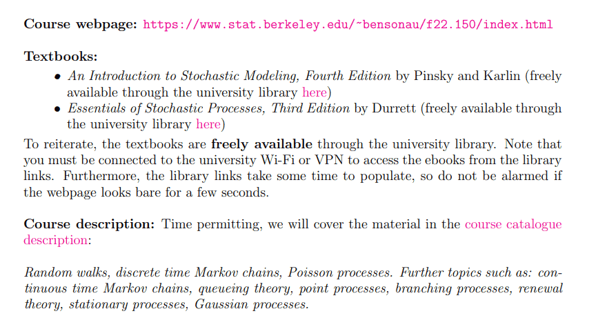
• An Introduction to Stochastic Modeling, Fourth Edition by Pinsky and Karlin (freely available through the university library here) • Essentials of Stochastic Processes, Third Edition by Durrett (freely available through the university library here) To reiterate, the textbooks are freely available through the university library. Note that you must be connected to the university Wi-Fi or VPN to access the ebooks from the library links. Furthermore, the library links take some time to populate, so do not be alarmed if the webpage looks bare for a few seconds.
统计代写|Stat 150: Stochastic Processes随机过程代考
Statistics-lab™可以为您提供berkeley.edu Stat 150: Stochastic Processes随机过程课程的代写代考和辅导服务! 请认准Statistics-lab™. Statistics-lab™为您的留学生涯保驾护航。