数学代写|MATH208 Operations Research
Statistics-lab™可以为您提供rochester.edu MATH208 Operations Research运筹学的代写代考和辅导服务!
MATH208 Operations Research课程简介
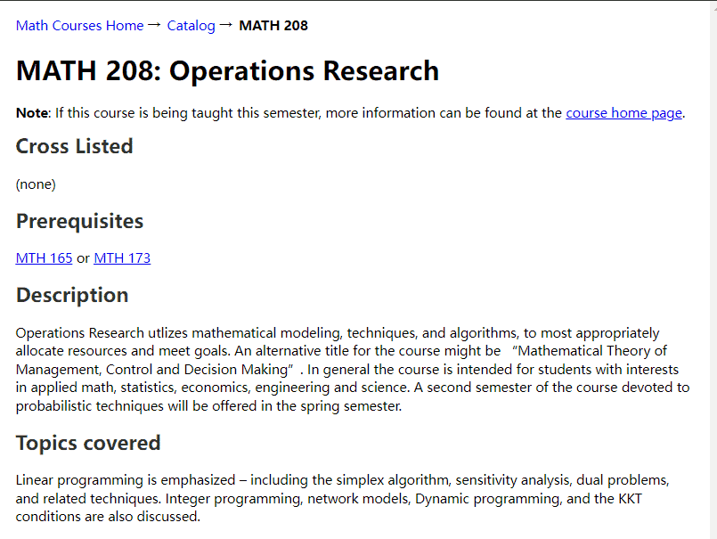
Operations Research utlizes mathematical modeling, techniques, and algorithms, to most appropriately allocate resources and meet goals. An alternative title for the course might be “Mathematical Theory of Management, Control and Decision Making” . In general the course is intended for students with interests in applied math, statistics, economics, engineering and science. A second semester of the course devoted to probabilistic techniques will be offered in the spring semester.
PREREQUISITES
Linear programming is a widely-used optimization technique that involves linear objective functions and linear constraints. The simplex algorithm is a widely-used algorithm for solving linear programming problems, and it involves moving from one feasible solution to another in an iterative fashion until an optimal solution is found. Sensitivity analysis involves examining the effects of changes in the objective function coefficients and constraint values on the optimal solution.
Dual problems are closely related to linear programming problems and involve the optimization of a dual objective function subject to dual constraints. The dual problem is used to provide information about the original problem, including bounds on the optimal objective value and information about the shadow prices of the constraints.
Integer programming is a type of linear programming that involves additional constraints that require the variables to take on integer values. Network models involve the modeling of complex systems using networks, such as transportation or communication systems. Dynamic programming is a powerful optimization technique that involves breaking down a problem into smaller subproblems and solving each subproblem in a recursive manner.
Finally, the KKT conditions are a set of necessary conditions for an optimization problem to have an optimal solution. These conditions involve the first-order conditions for optimality and the complementary slackness conditions, and they are used to analyze optimization problems and to derive insights about their solutions.
MATH208 Operations Research HELP(EXAM HELP, ONLINE TUTOR)
Give a dynamic programming algorithm for the following $0-1$ knapsack problem, where the $a_j$, the $b_j$, and $B$ are given positive integers:
$$
\begin{array}{ll}
\text { Maximize } & \sum_{j=1}^n a_j x_j \
\text { subject to } & \sum_{j=1}^n b_j x_j \leq B \
\text { and } & x_j \in{0,1} \text { for } 1 \leq j \leq n
\end{array}
$$
The $0-1$ knapsack problem is a classic problem in dynamic programming. We can solve it using dynamic programming by building a table of optimal solutions for subproblems. Let $K(i, w)$ be the maximum value that can be obtained by using items $1, 2, \ldots, i$ with a weight limit of $w$. The dynamic programming algorithm is as follows:
- Initialize a table $T$ with $n+1$ rows and $B+1$ columns, where $T[i][w]$ represents the maximum value that can be obtained by using items $1, 2, \ldots, i$ with a weight limit of $w$.
- Set $T[0][w] = 0$ for all $w$, since we cannot choose any items when there are no items available.
- For each item $i$ from $1$ to $n$, and for each weight $w$ from $0$ to $B$, compute the maximum value that can be obtained by either including or excluding item $i$. If item $i$ is excluded, then $T[i][w] = T[i-1][w]$. If item $i$ is included, then $T[i][w] = T[i-1][w-b_i] + a_i$ if $w \geq b_i$. Otherwise, we cannot include item $i$, so $T[i][w] = T[i-1][w]$.
- The maximum value that can be obtained using items $1, 2, \ldots, n$ with a weight limit of $B$ is given by $T[n][B]$.
The time complexity of this algorithm is $O(nB)$, since we need to compute $T[i][w]$ for $nB$ subproblems.
Here’s the Python code for the dynamic programming algorithm:
rCopy codedef knapsack(a, b, B):
    n = len(a)
    T = [[0 for _ in range(B+1)] for _ in range(n+1)]
    for i in range(1, n+1):
        for w in range(B+1):
            if b[i-1] <= w:
                T[i][w] = max(T[i-1][w], T[i-1][w-b[i-1]] + a[i-1])
            else:
                T[i][w] = T[i-1][w]
    return T[n][B]
To use this function, simply call knapsack(a, b, B) with the lists a and b containing the values and weights of each item, respectively, and B as the weight limit. The function returns the maximum value that can be obtained using the items subject to the weight limit.
(a) A manufacturer must decide how many microchips to include in each of the circuits $A, B$, and $C$ in an electronic system to maximize the probability that the system works over a given period of time. The system only works if in each circuit, at least one chip works. Both the circuits and the chips within a circuit work independently of one another. The probability that a chip fails within the scheduled time period is $0.2,0.3$, and 0.25 for the circuits $A, B$ and $C$. In all, no more than six chips can be included, and no circuit can have more than two. How can the manufacturer design the most reliable system?
(b) Use dynamic programming to solve the following problem:
$\begin{array}{ll}\text { Maximize } & x_1^{1 / 2} x_2 x_3^2 \ \text { subject to } & 0.5 x_1+x_2^2+4 x_3 \leq 15 \ \text { and } & x_1, x_2, x_3 \geq 0 \text { and integer. }\end{array}$
(a) Let $x_A, x_B, x_C$ be the number of chips included in circuits $A, B$, and $C$, respectively. We want to maximize the probability that the system works, which is given by $P = (1 – 0.2^{x_A})(1 – 0.3^{x_B})(1 – 0.25^{x_C})$. We can formulate the problem as an integer programming problem as follows:
\begin{align*} \text{maximize } & P \ \text{subject to } & x_A + x_B + x_C \leq 6 \ & x_A \leq 2, x_B \leq 2, x_C \leq 2 \ & x_A, x_B, x_C \geq 1 \end{align*}
We can use dynamic programming to solve this problem by building a table of optimal solutions for subproblems. Let $T(i, j, k)$ be the maximum probability that can be obtained by using at most $i$ chips in circuit $A$, at most $j$ chips in circuit $B$, and at most $k$ chips in circuit $C$. The dynamic programming algorithm is as follows:
- Initialize a table $T$ with dimensions $(3,3,7)$, where $T(i,j,k)$ represents the maximum probability that can be obtained by using at most $i$ chips in circuit $A$, at most $j$ chips in circuit $B$, and at most $k$ chips in circuit $C$.
- Set $T(1,1,1) = (1 – 0.2)^1 (1 – 0.3)^1 (1 – 0.25)^1 = 0.315$.
- For each $i$ from $1$ to $2$, for each $j$ from $1$ to $2$, and for each $k$ from $1$ to $6$, compute the maximum probability that can be obtained by either including or excluding a chip in each circuit. If a chip is excluded, then $T(i,j,k) = T(i,j,k)$. If a chip is included, then $T(i,j,k) = \max{T(i-1,j,k), T(i,j-1,k), T(i,j,k-1)} (1 – p_A^i)(1 – p_B^j)(1 – p_C^k)$, where $p_A, p_B, p_C$ are the probabilities of failure for circuits $A, B$, and $C$, respectively. If $i+j+k = 6$, then we must include the remaining chips in the circuit with the lowest failure probability to ensure that the system works, so $T(2,2,6) = (1 – p_C^6)(1 – p_B^{2})(1 – p_A^{2})$.
- The maximum probability that can be obtained using at most $2$ chips in circuit $A$, at most $2$ chips in circuit $B$, and at most $2$ chips in circuit $C$ is given by $\max{T(2,2,k)}$ for $1 \leq k \leq 6$.
The time complexity of this algorithm is $O(108)$, since we need to compute $T(i,j,k)$ for $3 \times 3 \times 6 = 54$ subproblems and $T(2,2,6)$.
(b) To use dynamic programming to solve this problem, we can follow these steps:
Textbooks
• An Introduction to Stochastic Modeling, Fourth Edition by Pinsky and Karlin (freely
available through the university library here)
• Essentials of Stochastic Processes, Third Edition by Durrett (freely available through
the university library here)
To reiterate, the textbooks are freely available through the university library. Note that
you must be connected to the university Wi-Fi or VPN to access the ebooks from the library
links. Furthermore, the library links take some time to populate, so do not be alarmed if
the webpage looks bare for a few seconds.

Statistics-lab™可以为您提供rochester.edu MATH208 Operations Research运筹学的代写代考和辅导服务! 请认准Statistics-lab™. Statistics-lab™为您的留学生涯保驾护航。