10 月 2022 - 统计代写答疑辅导

月度归档： 2022 年 10 月

计算机代写|编码理论代写Coding theory代考|ELEN90030

Posted on 2022年10月31日2022年10月31日 by statistics-lab

如果你也在怎样代写编码理论Coding theory这个学科遇到相关的难题，请随时右上角联系我们的24/7代写客服。

编码理论是研究编码的属性和它们各自对特定应用的适用性。编码被用于数据压缩、密码学、错误检测和纠正、数据传输和数据存储。

statistics-lab™ 为您的留学生涯保驾护航在代写编码理论Coding theory方面已经树立了自己的口碑, 保证靠谱, 高质且原创的统计Statistics代写服务。我们的专家在代写编码理论Coding theory代写方面经验极为丰富，各种代写编码理论Coding theory相关的作业也就用不着说。

我们提供的编码理论Coding theory及其相关学科的代写，服务范围广, 其中包括但不限于:

Statistical Inference 统计推断
Statistical Computing 统计计算
Advanced Probability Theory 高等概率论
Advanced Mathematical Statistics 高等数理统计学
(Generalized) Linear Models 广义线性模型
Statistical Machine Learning 统计机器学习
Longitudinal Data Analysis 纵向数据分析
Foundations of Data Science 数据科学基础

计算机代写|编码理论代写Coding theory代考|Distance and Weight

The error-correcting capability of a code is keyed directly to the concepts of Hamming distance and Hamming weight. ${ }^3$

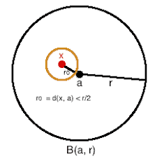
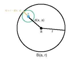
Definition 1.6.1 The (Hamming) distance between two vectors $\mathbf{x}, \mathbf{y} \in \mathbb{F}q^n$, denoted $\mathrm{d}{\mathbf{H}}(\mathbf{x}, \mathbf{y})$, is the number of coordinates in which $\mathbf{x}$ and $\mathbf{y}$ differ. The (Hamming) weight of $\mathbf{x} \in \mathbb{F}q^n$, denoted $\mathrm{wt}{\mathrm{H}}(\mathbf{x})$, is the number of coordinates in which $\mathbf{x}$ is nonzero.
Theorem 1.6.2 ([1008, Chapter 1.4]) The following hold.
(a) (nonnegativity) $\mathrm{d}{\mathrm{H}}(\mathbf{x}, \mathbf{y}) \geq 0$ for all $\mathbf{x}, \mathbf{y} \in \mathbb{F}_q^n$. (b) $\mathrm{d}{\mathrm{H}}(\mathbf{x}, \mathbf{y})=0$ if and only if $\mathbf{x}=\mathbf{y}$.
(c) (symmetry) $\mathrm{d}{\mathrm{H}}(\mathbf{x}, \mathbf{y})=\mathrm{d}{\mathrm{H}}(\mathbf{y}, \mathbf{x})$ for all $\mathbf{x}, \mathbf{y} \in \mathbb{F}q^n$. (d) (triangle inequality) $\mathrm{d}{\mathrm{H}}(\mathbf{x}, \mathbf{z}) \leq \mathrm{d}{\mathrm{H}}(\mathbf{x}, \mathbf{y})+\mathrm{d}{\mathrm{H}}(\mathbf{y}, \mathbf{z})$ for all $\mathbf{x}, \mathbf{y}, \mathbf{z} \in \mathbb{F}q^n$. (e) $\mathrm{d}{\mathrm{H}}(\mathbf{x}, \mathbf{y})=\mathrm{wt}{\mathrm{H}}(\mathbf{x}-\mathbf{y})$ for all $\mathbf{x}, \mathbf{y} \in \mathbb{F}_q^n$. (f) If $\mathbf{x}, \mathbf{y} \in \mathbb{F}_2^n$, then $$ w t_H(\mathbf{x}+\mathbf{y})=w{\mathrm{H}}(\mathbf{x})+w_{\mathrm{H}}(\mathbf{y})-2 w t_{\mathrm{H}}(\mathbf{x} \star \mathbf{y})
$$
where $\mathbf{x} \star \mathbf{y}$ is the vector in $\mathbb{F}2^n$ which has 1 s precisely in those coordinates where both $\mathbf{x}$ and $\mathbf{y}$ have $1 s$. (g) If $\mathbf{x}, \mathbf{y} \in \mathbb{F}_2^n$, then $\mathrm{wt}{\mathrm{H}}(\mathbf{x} \star \mathbf{y}) \equiv \mathbf{x} \cdot \mathbf{y}(\bmod 2)$. In particular, $\mathrm{wt}_{\mathrm{H}}(\mathbf{x}) \equiv \mathbf{x} \cdot \mathbf{x}(\bmod 2)$.

计算机代写|编码理论代写Coding theory代考|Puncturing, Extending, and Shortening Codes

There are several methods to obtain a longer or shorter code from a given code; while this can be done for both linear and nonlinear codes, we focus on linear ones. Two codes can be combined into a single code, for example as described in Section 1.11.

Definition 1.7.1 Let $\mathcal{C}$ be an $[n, k, d]q$ linear code with generator matrix $G$ and parity check matrix $H$. (a) For some $i$ with $1 \leq i \leq n$, let $\mathcal{C}^$ be the codewords of $\mathcal{C}$ with the $i^{\text {th }}$ component deleted. The resulting code, called a punctured code, is an $\left[n-1, k^, d^\right]$ code. If $d>1, k^=k$, and $d^=d$ unless $\mathcal{C}$ has a minimum weight codeword that is nonzero on coordinate $i$, in which case $d^=d-1$. If $d=1, k^=k$ and $d^=1$ unless $\mathcal{C}$ has a weight 1 codeword that is nonzero on coordinate $i$, in which case $k^=k-1$ and $d^ \geq 1$ as long as $\mathcal{C}^$ is nonzero. A generator matrix for $\mathcal{C}^$ is obtained from $G$ by deleting column $i ; G^$ will have dependent rows if $d^=1$ and $k^*=k-1$. Puncturing is often done on multiple coordinates in an analogous manner, one coordinate at a time.
(b) Define $\widehat{\mathcal{C}}=\left{c_1 c_2 \cdots c{n+1} \in \mathbb{F}q^{n+1} \mid c_1 c_2 \cdots c_n \in \mathcal{C}\right.$ where $\left.\sum{i=1}^{n+1} c_i=0\right}$, called the extended code. This is an $[n+1, k, \widehat{d}]_q$ code where $\widehat{d}=d$ or $d+1$. A generator matrix $\widehat{G}$ for $\widehat{\mathcal{C}}$ is obtained by adding a column on the right of $G$ so that every row sum in this $k \times(n+1)$ matrix is 0 . A parity check matrix $\widehat{H}$ for $\widehat{\mathcal{C}}$ is
$$
\widehat{H}=\left[\begin{array}{ccc|c}
1 & \cdots & 1 & 1 \
\hline & & 0 \
& H & & \vdots \
& & & 0
\end{array}\right] .
$$
(c) Let $S$ be any set of $s$ coordinates. Let $\mathcal{C}(S)$ be all codewords in $\mathcal{C}$ that are zero on $S$. Puncturing $\mathcal{C}(S)$ on $S$ results in the $\left[n-s, k_S, d_S\right]_q$ shortened code $\mathcal{C}_S$ where $d_S \geq d$. If $\mathcal{C}^{\perp}$ has minimum weight $d^{\perp}$ and $s<d^{\perp}$, then $k_S=k-s$.

编码理论代考

计算机代写|编码理论代写Coding theory代考|Distance and Weight

代码的纠错能力直接取决于汉明距离和汉明权重的概念。 3
定义 1.6.1 两个向量之间的 (汉明) 距离 $\mathbf{x}, \mathbf{y} \in \mathbb{F} q^n$ ，表示 $\mathrm{d} \mathbf{H}(\mathbf{x}, \mathbf{y})$ ，是其中的坐标数 $\mathbf{x}$ 和 $\mathbf{y}$ 不同。的（汉明) 权重 $\mathbf{x} \in \mathbb{F} q^n$ ，表示wtH $\left.\mathbf{x} \mathbf{x}\right)$, 是其中的坐标数 $\mathbf{x}$ 是非零的。
定理 1.6.2 ([1008, Chapter 1.4])以下成立。
(a) (非消极性) $\mathrm{dH}(\mathbf{x}, \mathbf{y}) \geq 0$ 对所有人 $\mathbf{x}, \mathbf{y} \in \mathbb{F}q^n$. (二) $\mathrm{dH}(\mathbf{x}, \mathbf{y})=0$ 当且仅当 $\mathbf{x}=\mathbf{y}$. (c) (对称) $\mathrm{dH}(\mathbf{x}, \mathbf{y})=\mathrm{dH}(\mathbf{y}, \mathbf{x})$ 对所有人 $\mathbf{x}, \mathbf{y} \in \mathbb{F} q^n$. (d) (三角不等式) $\mathrm{dH}(\mathbf{x}, \mathbf{z}) \leq \mathrm{dH}(\mathbf{x}, \mathbf{y})+\mathrm{dH}(\mathbf{y}, \mathbf{z})$ 对所有人 $\mathbf{x}, \mathbf{y}, \mathbf{z} \in \mathbb{F} q^n$. (和) $\mathrm{dH}(\mathbf{x}, \mathbf{y})=w \mathrm{wt}(\mathbf{x}-\mathbf{y})$ 对所有人 $\mathbf{x}, \mathbf{y} \in \mathbb{F}_q^n$. (f) 如果 $\mathbf{x}, \mathbf{y} \in \mathbb{F}_2^n$ ，然后 $$ w t_H(\mathbf{x}+\mathbf{y})=w \mathrm{H}(\mathbf{x})+w{\mathrm{H}}(\mathbf{y})-2 w t_{\mathrm{H}}(\mathbf{x} \star \mathbf{y})
$$
在哪里 $\mathbf{x} \star \mathbf{y}$ 是向量 $\mathbb{F} 2^n$ 在那些坐标中精确地有 $1 \mathrm{~s} \mathbf{x}$ 和 $\mathbf{y}$ 有 $1 s$. (g) 如果 $\mathbf{x}, \mathbf{y} \in \mathbb{F}2^n$ ，然后 $w t H(\mathbf{x} \star \mathbf{y}) \equiv \mathbf{x} \cdot \mathbf{y}(\bmod 2)$. 尤其是， $\mathrm{wt}{\mathrm{H}}(\mathbf{x}) \equiv \mathbf{x} \cdot \mathbf{x}(\bmod 2)$.

计算机代写|编码理论代写Coding theory代考|Puncturing, Extending, and Shortening Codes

有几种方法可以从给定的代码中获取更长或更短的代码；虽然伩对于线性和非线性代码都可以做到，但我们专注于线性代码。两个代码可以组合成一个代码，例如第 $1.11$ 节所述。
定义 $1.7 .1$ 让 $\mathcal{C}$ 豆 $[n, k, d] q$ 带有生成矩阵的线性代码 $G$ 和奇偶校验矩阵 $H$. (a) 对于一些 $i$ 和 $1 \leq i \leq n$ ，让数学 ${C}^{\wedge}$ 是的代码字 $\mathcal{C}$ 与 $i^{\text {th }}$ 组件被删除。生成的代码，称为打孔代码，是 $M$ left[n-1, $\left.\mathrm{k}^{\wedge}, \mathrm{d}^{\wedge} \backslash \mathrm{right}^2\right]$ 代码。如果 $d>1, k^{=} k$ ，和 $d^{=} d$ 除非 $\mathcal{C}$ 具有在坐标上非零的最小权重码字 $i$ ，在这种情况下 $d^{=} d-1$. 如果 $d=1, k^{=} k$ 和数学 {C}^ 是从 $G$ 通过删除列和 $\mathrm{G}^{\wedge}$ 如果 $d^{=} 1$ 和 $k^*=k-1$. 穿孔通常以类似的方式在多个坐标上进行，一次一个坐标。
(b) 定义得 $G$ 这样每一行总和 $k \times(n+1)$ 矩阵是 0 。奇偶校验矩阵 $\widehat{H}$ 为了 $\widehat{\mathcal{C}}$ 是
(c) 让 $S$ 是任何一组 $s$ 坐标。让 $\mathcal{C}(S)$ 是所有的代码字 $\mathcal{C}$ 是零 $S$. 穿刺 $\mathcal{C}(S)$ 上 $S$ 结果是 $\left[n-s, k_S, d_S\right]_q$ 缩短的代码 $\mathcal{C}_S$ 在哪里 $d_S \geq d$. 如果 $\mathcal{C}^{\perp}$ 有最小重量 $d^{\perp}$ 和 $s<d^{\perp}$ ，然后 $k_S=k-s$.

计算机代写|编码理论代写Coding theory代考请认准statistics-lab™

统计代写请认准statistics-lab™. statistics-lab™为您的留学生涯保驾护航。

金融工程代写

金融工程是使用数学技术来解决金融问题。金融工程使用计算机科学、统计学、经济学和应用数学领域的工具和知识来解决当前的金融问题，以及设计新的和创新的金融产品。

非参数统计代写

非参数统计指的是一种统计方法，其中不假设数据来自于由少数参数决定的规定模型；这种模型的例子包括正态分布模型和线性回归模型。

广义线性模型代考

广义线性模型（GLM）归属统计学领域，是一种应用灵活的线性回归模型。该模型允许因变量的偏差分布有除了正态分布之外的其它分布。

术语广义线性模型（GLM）通常是指给定连续和/或分类预测因素的连续响应变量的常规线性回归模型。它包括多元线性回归，以及方差分析和方差分析（仅含固定效应）。

有限元方法代写

有限元方法（FEM）是一种流行的方法，用于数值解决工程和数学建模中出现的微分方程。典型的问题领域包括结构分析、传热、流体流动、质量运输和电磁势等传统领域。

有限元是一种通用的数值方法，用于解决两个或三个空间变量的偏微分方程（即一些边界值问题）。为了解决一个问题，有限元将一个大系统细分为更小、更简单的部分，称为有限元。这是通过在空间维度上的特定空间离散化来实现的，它是通过构建对象的网格来实现的：用于求解的数值域，它有有限数量的点。边界值问题的有限元方法表述最终导致一个代数方程组。该方法在域上对未知函数进行逼近。[1] 然后将模拟这些有限元的简单方程组合成一个更大的方程系统，以模拟整个问题。然后，有限元通过变化微积分使相关的误差函数最小化来逼近一个解决方案。

tatistics-lab作为专业的留学生服务机构，多年来已为美国、英国、加拿大、澳洲等留学热门地的学生提供专业的学术服务，包括但不限于Essay代写，Assignment代写，Dissertation代写，Report代写，小组作业代写，Proposal代写，Paper代写，Presentation代写，计算机作业代写，论文修改和润色，网课代做，exam代考等等。写作范围涵盖高中，本科，研究生等海外留学全阶段，辐射金融，经济学，会计学，审计学，管理学等全球99%专业科目。写作团队既有专业英语母语作者，也有海外名校硕博留学生，每位写作老师都拥有过硬的语言能力，专业的学科背景和学术写作经验。我们承诺100%原创，100%专业，100%准时，100%满意。

随机分析代写

随机微积分是数学的一个分支，对随机过程进行操作。它允许为随机过程的积分定义一个关于随机过程的一致的积分理论。这个领域是由日本数学家伊藤清在第二次世界大战期间创建并开始的。

时间序列分析代写

随机过程，是依赖于参数的一组随机变量的全体，参数通常是时间。随机变量是随机现象的数量表现，其时间序列是一组按照时间发生先后顺序进行排列的数据点序列。通常一组时间序列的时间间隔为一恒定值（如1秒，5分钟，12小时，7天，1年），因此时间序列可以作为离散时间数据进行分析处理。研究时间序列数据的意义在于现实中，往往需要研究某个事物其随时间发展变化的规律。这就需要通过研究该事物过去发展的历史记录，以得到其自身发展的规律。

回归分析代写

多元回归分析渐进（Multiple Regression Analysis Asymptotics）属于计量经济学领域，主要是一种数学上的统计分析方法，可以分析复杂情况下各影响因素的数学关系，在自然科学、社会和经济学等多个领域内应用广泛。

MATLAB代写

MATLAB 是一种用于技术计算的高性能语言。它将计算、可视化和编程集成在一个易于使用的环境中，其中问题和解决方案以熟悉的数学符号表示。典型用途包括：数学和计算算法开发建模、仿真和原型制作数据分析、探索和可视化科学和工程图形应用程序开发，包括图形用户界面构建MATLAB 是一个交互式系统，其基本数据元素是一个不需要维度的数组。这使您可以解决许多技术计算问题，尤其是那些具有矩阵和向量公式的问题，而只需用 C 或 Fortran 等标量非交互式语言编写程序所需的时间的一小部分。MATLAB 名称代表矩阵实验室。MATLAB 最初的编写目的是提供对由 LINPACK 和 EISPACK 项目开发的矩阵软件的轻松访问，这两个项目共同代表了矩阵计算软件的最新技术。MATLAB 经过多年的发展，得到了许多用户的投入。在大学环境中，它是数学、工程和科学入门和高级课程的标准教学工具。在工业领域，MATLAB 是高效研究、开发和分析的首选工具。MATLAB 具有一系列称为工具箱的特定于应用程序的解决方案。对于大多数 MATLAB 用户来说非常重要，工具箱允许您学习和应用专业技术。工具箱是 MATLAB 函数（M 文件）的综合集合，可扩展 MATLAB 环境以解决特定类别的问题。可用工具箱的领域包括信号处理、控制系统、神经网络、模糊逻辑、小波、仿真等。

R语言代写	问卷设计与分析代写
PYTHON代写	回归分析与线性模型代写
MATLAB代写	方差分析与试验设计代写
STATA代写	机器学习/统计学习代写
SPSS代写	计量经济学代写
EVIEWS代写	时间序列分析代写
EXCEL代写	深度学习代写
SQL代写	各种数据建模与可视化代写

计算机代写|编码理论代写Coding theory代考|MATH597

Posted on 2022年10月31日2022年10月31日 by statistics-lab

如果你也在怎样代写编码理论Coding theory这个学科遇到相关的难题，请随时右上角联系我们的24/7代写客服。

编码理论是研究编码的属性和它们各自对特定应用的适用性。编码被用于数据压缩、密码学、错误检测和纠正、数据传输和数据存储。

我们提供的编码理论Coding theory及其相关学科的代写，服务范围广, 其中包括但不限于:

Statistical Inference 统计推断
Statistical Computing 统计计算
Advanced Probability Theory 高等概率论
Advanced Mathematical Statistics 高等数理统计学
(Generalized) Linear Models 广义线性模型
Statistical Machine Learning 统计机器学习
Longitudinal Data Analysis 纵向数据分析
Foundations of Data Science 数据科学基础

计算机代写|编码理论代写Coding theory代考|Generator and Parity Check Matrices

When choosing between linear and nonlinear codes, the added algebraic structure of linear codes often makes them easier to describe and use. Generally, a linear code is defined by giving either a generator or a parity check matrix.

Definition 1.4.1 Let $\mathcal{C}$ be an $[n, k]_q$ linear code. A generator matrix $G$ for $\mathcal{C}$ is any $G \in \mathbb{F}_q^{k \times n}$ whose row span is $\mathcal{C}$. Because any $k$-dimensional subspace of $\mathbb{F}_q^n$ is the kernel of some linear transformation from $\mathbb{F}_q^n$ onto $\mathbb{F}_q^{n-k}$, there exists $H \in \mathbb{F}_q^{(n-k) \times n}$, with independent many, is called a parity check matrix of $\mathcal{C}$.

Example 1.4.2 Continuing with Example 1.3.2, there are several generator matrices for $\mathcal{C}_1$ including
$$
G_1=\left[\begin{array}{llll}
1 & 0 & 0 & 1 \
0 & 1 & 0 & 1 \
0 & 0 & 1 & 1
\end{array}\right], G_1^{\prime}=\left[\begin{array}{cccc}
1 & 1 & 1 & 1 \
1 & 1 & 0 & 0 \
0 & 1 & 1 & 0
\end{array}\right] \text {, and } G_1^{\prime \prime}=\left[\begin{array}{cccc}
1 & 1 & 0 & 0 \
0 & 1 & 1 & 0 \
0 & 0 & 1 & 1
\end{array}\right] .
$$
Remark 1.4.3 Any matrix obtained by elementary row operations from a generator matrix for a code remains a generator matrix of that code.

Remark 1.4.4 By Definition 1.4.1, the rows of $G$ form a basis of $\mathcal{C}$, and the rows of $H$ are independent. At times, the requirement may be relaxed so that the rows of $G$ are only required to span $\mathcal{C}$. Similarly, the requirement that the rows of $H$ be independent may be dropped as long as $\mathcal{C}=\left{\mathbf{c} \in \mathbb{F}_q^n \mid H \mathbf{c}^{\top}=0^{\top}\right}$ remains true.

计算机代写|编码理论代写Coding theory代考|Orthogonality

In this section we introduce the concept of codes over finite fields. We begin with some notation.

The set of $n$-tuples with entries in $\mathbb{F}_q$ forms an $n$-dimensional vector space, denoted $\mathbb{F}_q^n=\left{x_1 x_2 \cdots x_n \mid x_i \in \mathbb{F}_q, 1 \leq i \leq n\right}$, under componentwise addition of $n$-tuples and componentwise multiplication of $n$-tuples by scalars in $\mathbb{F}_q$. The vectors in $\mathbb{F}_q^n$ will often be denoted using bold Roman characters $\mathbf{x}=x_1 x_2 \cdots x_n$. The vector $\mathbf{0}=00 \cdots 0$ is the zero vector in $\mathbb{F}_q^n$.

There is a natural inner product on $\mathbb{F}q^n$ that often proves useful in the study of codes. ${ }^2$ Definition 1.5.1 The ordinary inner product, also called the Euclidean inner product, on $\mathbb{F}_q^n$ is defined by $\mathbf{x} \cdot \mathbf{y}=\sum{i=1}^n x_i y_i$ where $\mathbf{x}=x_1 x_2 \cdots x_n$ and $\mathbf{y}=y_1 y_2 \cdots y_n$. Two vectors $\mathbf{x}, \mathbf{y} \in \mathbb{F}_q^n$ are orthogonal if $\mathbf{x} \cdot \mathbf{y}=0$. If $\mathcal{C}$ is an $[n, k]_q$ code,
$$
\mathcal{C}^{\perp}=\left{\mathbf{x} \in \mathbb{F}_q^n \mid \mathbf{x} \cdot \mathbf{c}=0 \text { for all } \mathbf{c} \in \mathcal{C}\right}
$$ is the orthogonal code or dual code of $\mathcal{C}$. $\mathcal{C}$ is self-orthogonal if $\mathcal{C} \subseteq \mathcal{C}^{\perp}$ and self-dual if $\mathcal{C}=\mathcal{C}^{\perp}$.

Theorem 1.5.2 ([1323, Chapter 1.8 $])$ Let $\mathcal{C}$ be an $[n, k]_q$ code with generator and parity check matrices $G$ and $H$, respectively. Then $\mathcal{C}^{\perp}$ is an $[n, n-k]_q$ code with generator and parity check matrices $H$ and $G$, respectively. Additionally $\left(\mathcal{C}^{\perp}\right)^{\perp}=\mathcal{C}$. Furthermore $\mathcal{C}$ is self-dual if and only if $\mathcal{C}$ is self-orthogonal and $k=\frac{n}{2}$.

Example 1.5.3 $\mathcal{C}2$ from Example $1.4 .8$ is a $[4,2]_2$ self-dual code with generator and parity check matrices both equal to $$ \left[\begin{array}{llll} 1 & 1 & 0 & 0 \ 0 & 0 & 1 & 1 \end{array}\right] \text {. } $$ The dual of the Hamming $[7,4]_2$ code in Example 1.4.9 is a $[7,3]_2$ code $\mathcal{H}{3,2}^{\perp} . H_{3,2}$ is a generator matrix of $\mathcal{H}{3,2}^{\perp}$. As every row of $H{3,2}$ is orthogonal to itself and every other row of $H_{3,2}, \mathcal{H}{3,2}^{\perp}$ is self-orthogonal. As $\mathcal{H}{3,2}^{\perp}$ has dimension 3 and $\left(\mathcal{H}{3,2}^{\perp}\right)^{\perp}=\mathcal{H}{3,2}$ has dimension 4, $\mathcal{H}_{3,2}^{\perp}$ is not self-dual.

编码理论代考

计算机代写|编码理论代写Coding theory代考|Generator and Parity Check Matrices

在线性码和非线性码之间进行选择时，线性码添加的代数结构通常使它们更易于描述和使用。通常，通过给出生成器或奇偶校验矩阵来定义线性码。
定义 $1.4 .1$ 让 $\mathcal{C}$ 豆 $[n, k]_q$ 线性码。生成矩阵 $G$ 为了 $\mathcal{C}$ 是任何 $G \in \mathbb{F}_q^{k \times n}$ 其行跨度为 $\mathcal{C}$. 因为任何 $k$-维子空间 $\mathbb{F}_q^n$ 是一些线性变换的核 $\mathbb{F}_q^n$ 到 $\mathbb{F}_q^{n-k}$ ，那里存在 $H \in \mathbb{F}_q^{(n-k) \times n}$ ，具有独立的许多，称为奇偶校验矩阵 $\mathcal{C}$.
示例 1.4.2 继续示例 1.3.2，有几个生成器矩阵 $\mathcal{C}_1$ 包含
备注 $1.4 .3$ 通过基本行操作从代码的生成矩阵获得的任何矩阵仍然是该代码的生成矩阵。
备注 1.4.4 根据定义 1.4.1，行 $G$ 形成一个基础 $\mathcal{C}$, 和的行 $H$ 是独立的。有时，要求可能会放宽，以便 $G$ 只需要跨越
$\mathcal{C}$. 同样，要求的行 $H$ 只要是独立的就可以被丟弃

计算机代写|编码理论代写Coding theory代考|Orthogonality

在本节中，我们介绍有限域上的码的概念。我们从一些符号开始。
该组 $n$ – 包含条目的元组 $\mathbb{F}q$ 形成一个n维向量空间，表示为和组件乘法 $n$ – 元组中的标量 $\mathbb{F}_q$. 中的向量 $\mathbb{F}_q^n$ 通常使用粗体罗马字符表示 $\mathbf{x}=x_1 x_2 \cdots x_n$. 向量 $\mathbf{0}=00 \cdots 0$ 是零向量 $\mathbb{F}_q^n$. 有天然内积 $\mathbb{F} q^n$ 这通常在代码研究中被证明是有用的。 ${ }^2$ 定义 $1.5 .1$ 普通内积，也称为欧几里得内积，在 $\mathbb{F}_q^n$ 定义为 $\mathbf{x} \cdot \mathbf{y}=\sum i=1^n x_i y_i$ 在哪里 $\mathbf{x}=x_1 x_2 \cdots x_n$ 和 $\mathbf{y}=y_1 y_2 \cdots y_n$. 两个向量 $\mathbf{x}, \mathbf{y} \in \mathbb{F}_q^n$ 是正交的，如果 $\mathbf{x} \cdot \mathbf{y}=0$. 如果 $\mathcal{C}$ 是一个 $[n, k]_q$ 代码，是正交码或双码 $\mathcal{C} . \mathcal{C}$ 是自正交的，如果 $\mathcal{C} \subseteq \mathcal{C}^{\perp}$ 和自对偶如果 $\mathcal{C}=\mathcal{C}^{\perp}$. 定理 $1.5 .2$ ([1323，第 $1.8$ 章 $]$ 让 $\mathcal{C}$ 豆 $[n, k]_q$ 带有生成器和奇偶校验矩阵的代码 $G$ 和 $H$ ，分别。然后 $\mathcal{C}^{\perp}$ 是一个 $[n, n-k]_q$ 带有生成器和奇偶校验矩阵的代码 $H$ 和 $G$ ，分别。此外 $\left(\mathcal{C}^{\perp}\right)^{\perp}=\mathcal{C}$. 此外 $\mathcal{C}$ 是自对偶当且仅当 $\mathcal{C}{\text {是自 }}$ 正交的并且 $k=\frac{n}{2}$.
示例 1.5.3C2来自示例 $1.4 .8$ 是一个 $[4,2]2$ 具有生成器和奇偶校验矩阵的自对偶代码都等于 $$ \left[\begin{array}{llllllll} 1 & 1 & 0 & 0 & 0 & 0 & 1 & 1 \end{array}\right] . $$ 汉明的对偶 $[7,4]_2$ 示例 $1.4 .9$ 中的代码是 $[7,3]_2$ 代码 $\mathcal{H} 3,2^{\perp} . H{3,2}$ 是一个生成矩阵 $\mathcal{H} 3,2^{\perp}$. 作为每一行 $H 3,2$ 正交于自身和每隔一行 $H_{3,2}, \mathcal{H} 3,2^{\perp}$ 是自正交的。作为 $\mathcal{H} 3,2^{\perp}$ 具有维度 3 和 $\left(\mathcal{H} 3,2^{\perp}\right)^{\perp}=\mathcal{H} 3,2$ 维度为 4 ， $\mathcal{H}_{3,2}^{\perp}$ 不是自对偶。

统计代写请认准statistics-lab™. statistics-lab™为您的留学生涯保驾护航。

金融工程代写

非参数统计代写

非参数统计指的是一种统计方法，其中不假设数据来自于由少数参数决定的规定模型；这种模型的例子包括正态分布模型和线性回归模型。

广义线性模型代考

广义线性模型（GLM）归属统计学领域，是一种应用灵活的线性回归模型。该模型允许因变量的偏差分布有除了正态分布之外的其它分布。

有限元方法代写

随机分析代写

时间序列分析代写

回归分析代写

MATLAB代写

R语言代写	问卷设计与分析代写
PYTHON代写	回归分析与线性模型代写
MATLAB代写	方差分析与试验设计代写
STATA代写	机器学习/统计学习代写
SPSS代写	计量经济学代写
EVIEWS代写	时间序列分析代写
EXCEL代写	深度学习代写
SQL代写	各种数据建模与可视化代写

计算机代写|编码理论代写Coding theory代考|CS294-226

Posted on 2022年10月31日2022年10月31日 by statistics-lab

如果你也在怎样代写编码理论Coding theory这个学科遇到相关的难题，请随时右上角联系我们的24/7代写客服。

编码理论是研究编码的属性和它们各自对特定应用的适用性。编码被用于数据压缩、密码学、错误检测和纠正、数据传输和数据存储。

我们提供的编码理论Coding theory及其相关学科的代写，服务范围广, 其中包括但不限于:

Statistical Inference 统计推断
Statistical Computing 统计计算
Advanced Probability Theory 高等概率论
Advanced Mathematical Statistics 高等数理统计学
(Generalized) Linear Models 广义线性模型
Statistical Machine Learning 统计机器学习
Longitudinal Data Analysis 纵向数据分析
Foundations of Data Science 数据科学基础

计算机代写|编码理论代写Coding theory代考|Finite Fields

Finite fields play an essential role in coding theory. The theory and construction of finite fields can be found, for example, in [1254] and [1408, Chapter 2]. Finite fields, as related specifically to codes, are described in [1008, 1323, 1602]. In this section we give a brief introduction.

Definition 1.2.1 A field $F$ is a nonempty set with two binary operations, denoted $+$ and , satisfying the following properties.
(a) For all $\alpha, \beta, \gamma \in \mathbb{F}, \alpha+\beta \in \mathbb{F}, \alpha \cdot \beta \in \mathbb{F}, \alpha+\beta=\beta+\alpha, \alpha \cdot \beta=\beta \cdot \alpha, \alpha+(\beta+\gamma)=(\alpha+\beta)+\gamma$, $\alpha \cdot(\beta \cdot \gamma)=(\alpha \cdot \beta) \cdot \gamma$, and $\alpha \cdot(\beta+\gamma)=\alpha \cdot \beta+\alpha \cdot \gamma$.
(b) $\mathbb{F}$ possesses an additive identity or zero, denoted 0 , and a multiplicative identity or unity, denoted 1 , such that $\alpha+0=\alpha$ and $\alpha \cdot 1=\alpha$ for all $\alpha \in \mathbb{F}_q$.
(c) For all $\alpha \in \mathbb{F}$ and all $\beta \in \mathbb{F}$ with $\beta \neq 0$, there exists $\alpha^{\prime} \in \mathbb{F}$, called the additive inverse of $\alpha$, and $\beta^* \in \mathbb{F}$, called the multiplicative inverse of $\beta$, such that $\alpha+\alpha^{\prime}=0$ and $\beta \cdot \beta^*=1$

The additive inverse of $\alpha$ will be denoted $-\alpha$, and the multiplicative inverse of $\beta$ will be denoted $\beta^{-1}$. Usually the multiplication operation will be suppressed; that is, $\alpha \cdot \beta$ will be denoted $\alpha \beta$. If $n$ is a positive integer and $\alpha \in \mathbb{F}, n \alpha=\alpha+\alpha+\cdots+\alpha\left(n\right.$ times), $\alpha^n=\alpha \alpha \cdots \alpha$ ( $n$ times), and $\alpha^{-n}=\alpha^{-1} \alpha^{-1} \cdots \alpha^{-1}$ ( $n$ times when $\alpha \neq 0$ ). Also $\alpha^0=1$ if $\alpha \neq 0$. The usual rules of exponentiation hold. If $\mathbb{F}$ is a finite set with $q$ elements, $\mathbb{F}$ is called a finite field of order $q$ and denoted $\mathbb{F}_q$.

Example 1.2.2 Fields include the rational numbers $\mathbb{Q}$, the real numbers $\mathbb{R}$, and the complex numbers $\mathbb{C}$. Finite fields include $\mathbb{Z}_p$, the set of integers modulo $p$, where $p$ is a prime.

计算机代写|编码理论代写Coding theory代考|Codes

In this section we introduce the concept of codes over finite fields. We begin with some notation.

For positive integers $m$ and $n, \mathbb{F}q^{m \times n}$ denotes the set of all $m \times n$ matrices with entries in $\mathbb{F}_q$. The matrix in $\mathbb{F}_q^{m \times n}$ with all entries 0 is the zero matrix denoted $\mathbf{0}{m \times n}$. The identity matrix of $\mathbb{F}q^{n \times n}$ will be denoted $I_n$. If $A \in \mathbb{F}_q^{m \times n}, A^{\top} \in \mathbb{F}_q^{n \times m}$ will denote the transpose of $A$. If $\mathbf{x} \in \mathbb{F}_q^m$, $\mathbf{x}^{\top}$ will denote $\mathbf{x}$ as a column vector of length $m$, that is, an $m \times 1$ matrix. The column vector $\mathbf{0}^{\top}$ and the $m \times 1$ matrix $\mathbf{0}{m \times 1}$ are the same.
If $S$ is any finite set, its order or size is denoted $|S|$.
Definition 1.3.1 A subset $\mathcal{C} \subseteq \mathbb{F}_q^n$ is called a code of length $n$ over $\mathbb{F}_q ; \mathbb{F}_q$ is called the alphabet of $\mathcal{C}$, and $\mathbb{F}_q^n$ is the ambient space of $\mathcal{C}$. Codes over $\mathbb{F}_q$ are also called $q$-ary codes. If the alphabet is $\mathbb{F}_2, \mathcal{C}$ is binary. If the alphabet is $\mathbb{F}_3, \mathcal{C}$ is ternary. The vectors in $\mathcal{C}$ are the codewords of $\mathcal{C}$. If $\mathcal{C}$ has $M$ codewords (that is, $|\mathcal{C}|=M$ ) $\mathcal{C}$ is denoted an $(n, M)_q$ code, or, more simply, an $(n, M)$ code when the alphabet $\mathbb{F}_q$ is understood. If $\mathcal{C}$ is a linear subspace of $\mathbb{F}_q^n$, that is $\mathcal{C}$ is closed under vector addition and scalar multiplication, $\mathcal{C}$ is called a linear code of length $n$ over $\mathbb{F}_q$. If the dimension of the linear code $\mathcal{C}$ is $k, \mathcal{C}$ is denoted an $[n, k]_q$ code, or, more simply, an $[n, k]$ code. An $(n, M)_q$ code that is also linear is an $[n, k]_q$ code where $M=q^k$. An $(n, M)_q$ code may be referred to as an unrestricted code; a specific unrestricted code may be either linear or nonlinear. When referring to a code, expressions such as $(n, M),(n, M)_q,[n, k]$, or $[n, k]_q$ are called the parameters of the coodé.

Example 1.3.2 Let $\mathcal{C}={1100,1010,1001,0110,0101,0011} \subseteq \mathbb{F}_2^4$. Then $\mathcal{C}$ is a $(4,6)_2$ binary nonlinear code. Let $\mathcal{C}_1=\mathcal{C} \cup{0000,1111}$. Then $\mathcal{C}_1$ is a $(4,8)_2$ binary linear code. As $\mathcal{C}_1$ is a subspace of $\mathbb{F}_2^4$ of dimension $3, \mathcal{C}_1$ is also a $[4,3]_2$ code.

编码理论代考

计算机代写|编码理论代写Coding theory代考|Finite Fields

有限域在编码理论中起着至关重要的作用。例如，在 [1254] 和 [1408，第 2 章] 中可以找到有限域的理论和构造。在 $[1008,1323,1602]$ 中描述了具体与代码相关的有限域。本节我们做一个简单的介绍。
定义 $1.2 .1$ 一个字段 $F$ 是具有两个二元运算的非空集，记为 $+$ 和，满足以下性质。
(a) 对所有人
$\alpha, \beta, \gamma \in \mathbb{F}, \alpha+\beta \in \mathbb{F}, \alpha \cdot \beta \in \mathbb{F}, \alpha+\beta=\beta+\alpha, \alpha \cdot \beta=\beta \cdot \alpha, \alpha+(\beta+\gamma)=(\alpha+\beta)+\gamma$ ，
$\alpha \cdot(\beta \cdot \gamma)=(\alpha \cdot \beta) \cdot \gamma ，$ 和 $\alpha \cdot(\beta+\gamma)=\alpha \cdot \beta+\alpha \cdot \gamma$.
(二) $\mathbb{F}$ 拥有一个加法单位或零，表示为 0 ，和一个乘法单位或单位，表示为 1 ，使得 $\alpha+0=\alpha$ 和 $\alpha \cdot 1=\alpha$ 对所有人 $\alpha \in \mathbb{F}_q$.
(c) 对所有人 $\alpha \in \mathbb{F}$ 和所有 $\beta \in \mathbb{F}$ 和 $\beta \neq 0$ ，那里存在 $\alpha^{\prime} \in \mathbb{F}$ ，称为加法逆 $\alpha$ ，和 $\beta^* \in \mathbb{F}$ ，称为乘法逆 $\beta$ ，这样 $\alpha+\alpha^{\prime}=0$ 和 $\beta \cdot \beta^*=1$
的加法逆 $\alpha$ 将表示 $-\alpha$ ，和乘法逆 $\beta$ 将表示 $\beta^{-1}$. 通常乘法运算会被抑制；那是， $\alpha \cdot \beta$ 将表示 $\alpha \beta$. 如果 $n$ 是一个正整数并且 $\alpha \in \mathbb{F}, n \alpha=\alpha+\alpha+\cdots+\alpha$ ( $n$ 次) ， $\alpha^n=\alpha \alpha \cdots \alpha(n$ 次 $)$ ，和 $\alpha^{-n}=\alpha^{-1} \alpha^{-1} \cdots \alpha^{-1}(n$ 有时 $\alpha \neq 0)$ 。还 $\alpha^0=1$ 如果 $\alpha \neq 0$. 通常的求幂规则成立。如果 $\mathbb{F}$ 是一个有限集 $q$ 元素， $\mathbb{F}$ 称为有限序域 $q$ 并表示 $\mathbb{F}_q$

计算机代写|编码理论代写Coding theory代考|Codes

在本节中，我们介绍有限域上的码的概念。我们从一些符号开始。
该组 $n$ – 包含条目的元组 $\mathbb{F}_q$ 形成一个 $n$ 维向量空间，表示为和组件乘法 $n$ – 元组中的标量 $\mathbb{F}_q$. 中的向量 $\mathbb{F}_q^n$ 通常使用粗体罗马字符表示 $\mathbf{x}=x_1 x_2 \cdots x_n$. 向量 $0=00 \cdots 0$ 是零向量 $\mathbb{F}_q^n$
对于正整数 $m$ 和 $n, \mathbb{F} q^{m \times n}$ 表示所有的集合 $m \times n$ 包含条目的矩阵 $\mathbb{F}_q$. 中的矩阵 $\mathbb{F}_q^{m \times n}$ 所有条目 0 是表示的零矩阵 $0 m \times n$. 的单位矩阵 $\mathbb{F} q^{n \times n}$ 将表示 $I_n$. 如果 $A \in \mathbb{F}_q^{m \times n}, A^{\top} \in \mathbb{F}_q^{n \times m}$ 将表示转置 $A$. 如果 $\mathbf{x} \in \mathbb{F}_q^m$ ， $\mathbf{x}^{\top}$ 将表示 $\mathbf{x}$ 作为长度的列向量 $m$ ，也就是说，一个 $m \times 1$ 矩阵。列向量 $\boldsymbol{0}^{\top}$ 和 $m \times 1$ 矩阵 $\mathbf{0} m \times 1$ 是相同的。如果 $S$ 是任何有限集，它的顺序或大小表示 $|S|$.
定义 1.3.1 一个子集 $\mathcal{C} \subseteq \mathbb{F}_q^n$ 称为长度码 $n$ 超过 $\mathbb{F}_q ; \mathbb{F}_q$ 被称为字母表 $\mathcal{C}$ ，和 $\mathbb{F}_q^n$ 是环境空间 $\mathcal{C}$. 代码结束 $\mathbb{F}_q$ 也被称为 $q$ -ary 代码。如果字母表是 $\mathbb{F}_2, \mathcal{C}$ 是二进制的。如果字母表是 $\mathbb{F}_3, \mathcal{C}$ 是三元的。中的向量 $\mathcal{C}$ 是的代码字 $\mathcal{C}$. 如果 $\mathcal{C}$ 有 $M$ 码字 (即 $|\mathcal{C}|=M) \mathcal{C}$ 表示为 $(n, M)_q$ 代码，或者更简单地说，一 $(n, M)$ 码当字母 $\mathbb{F}$ 被理解。如果 $\mathcal{C}$ 是一个线性子空间 $\mathbb{F}_q^n$ ，那是 $\mathcal{C}$ 在向量加法和标量乘法下是闭合的， $\mathcal{C}$ 称为长度的线性码 $n$ 超过 $\mathbb{F}_q$. 如果线性码的维数 $\mathcal{C}$ 是 $k, \mathcal{C}$ 表示为 $[n, k]_q$ 代码，或者更简单地说，一个 $[n, k]$ 代码。一个 $(n, M)_q$ 也是线性的代码是 $[n, k]_q$ 代码在哪里 $M=q^k$. 一个 $(n, M)_q$ 代码可以称为不受限制的代码; 一个特定的无限制代码可以是线性的也可以是非线性的。引用代码时，诸如 $(n, M),(n, M)_q,[n, k]$ ，或者 $[n, k]_q$ 被称为 coodé 的参数。
示例 $1.3 .2$ 让 $\mathcal{C}=1100,1010,1001,0110,0101,0011 \subseteq \mathbb{F}_2^4$. 然后 $\mathcal{C}$ 是一个 $(4,6)_2$ 二进制非线性码。让 $\mathcal{C}_1=\mathcal{C} \cup 0000,1111$. 然后 $\mathcal{C}_1$ 是一个 $(4,8)_2$ 二进制线性码。作为 $\mathcal{C}_1$ 是一个子空间 $\mathbb{F}_2^4$ 维度的 $3, \mathcal{C}_1$ 也是一个 $[4,3]_2$ 代码。

统计代写请认准statistics-lab™. statistics-lab™为您的留学生涯保驾护航。

金融工程代写

非参数统计代写

非参数统计指的是一种统计方法，其中不假设数据来自于由少数参数决定的规定模型；这种模型的例子包括正态分布模型和线性回归模型。

广义线性模型代考

广义线性模型（GLM）归属统计学领域，是一种应用灵活的线性回归模型。该模型允许因变量的偏差分布有除了正态分布之外的其它分布。

有限元方法代写

随机分析代写

时间序列分析代写

回归分析代写

MATLAB代写

R语言代写	问卷设计与分析代写
PYTHON代写	回归分析与线性模型代写
MATLAB代写	方差分析与试验设计代写
STATA代写	机器学习/统计学习代写
SPSS代写	计量经济学代写
EVIEWS代写	时间序列分析代写
EXCEL代写	深度学习代写
SQL代写	各种数据建模与可视化代写

数学代写|泛函分析作业代写Functional Analysis代考|МАTH3402

Posted on 2022年10月31日2022年10月31日 by statistics-lab

如果你也在怎样代写泛函分析Functional Analysis这个学科遇到相关的难题，请随时右上角联系我们的24/7代写客服。

泛函分析，数学分析的分支，处理函数，或函数的函数。它作为一个独立的领域出现在20世纪，当时人们意识到不同的数学过程，从算术到微积分程序，表现出非常相似的特性。

statistics-lab™ 为您的留学生涯保驾护航在代写泛函分析Functional Analysis方面已经树立了自己的口碑, 保证靠谱, 高质且原创的统计Statistics代写服务。我们的专家在代写泛函分析Functional Analysis代写方面经验极为丰富，各种代写泛函分析Functional Analysis相关的作业也就用不着说。

我们提供的泛函分析Functional Analysis及其相关学科的代写，服务范围广, 其中包括但不限于:

Statistical Inference 统计推断
Statistical Computing 统计计算
Advanced Probability Theory 高等概率论
Advanced Mathematical Statistics 高等数理统计学
(Generalized) Linear Models 广义线性模型
Statistical Machine Learning 统计机器学习
Longitudinal Data Analysis 纵向数据分析
Foundations of Data Science 数据科学基础

数学代写|泛函分析作业代写Functional Analysis代考|МАTH3402

数学代写|泛函分析作业代写Functional Analysis代考|Baire’s category theorem

Proof Suppose that the metric space $X=\bigcup_{n=1}^{\infty} A_n$, where $A_n$ are nowhere dense. We are going to create a nested sequence of balls whose centers form a nonconvergent Cauchy sequence, as follows: To start with, $\bar{A}1 \neq X$ so its exterior contains a ball $B{r_1}\left(x_1\right) \subseteq\left(A_1\right)^{\mathrm{C}}$. Now $A_2$ contains no balls, so the open set $\left(\bar{A}2\right)^{\mathrm{C}} \cap B{r_1}\left(x_1\right)$ is non-empty and there is a ball $B_{r_2}\left(x_2\right) \subseteq\left(\bar{A}2\right)^{\mathrm{C}} \cap B{r_1}\left(x_1\right)$.
$$
B_{r_{n+1}}\left[x_{n+1}\right] \subseteq B_{r_n}\left(x_n\right) \quad\left(\text { e.g. } r_{n+1}n$ we have $x_m \in B_{r_{n+1}}\left(x_{n+1}\right)$ and taking the limit $x_m \rightarrow x$ we find $x \in B_{r_{n+1}}\left[x_{n+1}\right] \subseteq B_{r_n}\left(x_n\right)$. Since this holds for any $n$ we obtain $$
x \in \bigcap_n B_{r_n}\left(x_n\right) \subseteq \bigcap_n\left(\bar{A}_n\right)^{\mathrm{C}}=\left(\bigcup_n \bar{A}_n\right)^{\mathrm{C}} \subseteq\left(\bigcup_n A_n\right)^{\mathrm{C}}=X^{\mathrm{C}}=\varnothing
$$
a contradiction. Having constructed a non-convergent Cauchy sequence, $X$ must be incomplete.

数学代写|泛函分析作业代写Functional Analysis代考|Uniformly Continuous Maps

We have seen that a continuous function need not preserve completeness, or even Cauchy sequences. If one analyzes the root of the problem, one finds that its resolution lies in the following strengthening of continuity:
Definition $4.11$
A function $f: X \rightarrow Y$ is said to be uniformly continuous when
$$
\forall \epsilon>0, \exists \delta>0, \forall x \in X, \quad f B_\delta(x) \subseteq B_\epsilon(f(x)) .
$$
The difference from continuity is that, here, $\delta$ is independent of $x$.
Easy Consequences

Uniformly continuous functions are continuous.
But not every continuous map is uniformly so; an example is $f(x):=1 / x$ on ] $0, \infty[$.
The composition of uniformly continuous maps is again uniformly continuous. Proof $\forall \epsilon>0, \exists \delta, \delta^{\prime}>0, \quad \forall x, g\left(f\left(B_\delta(x)\right)\right) \subseteq g\left(B_{\delta^{\prime}}(f(x))\right) \subseteq B_\epsilon(g(f(x)))$.
The key properties of uniformly continuous maps are the following two propositions:
Proposition $4.12$
A uniformly continuous function maps any Cauchy sequence to a Cauchy sequence.
Proof By definition $f: X \rightarrow Y$ is uniformly continuous when
$$
\forall \epsilon>0, \exists \delta>0, \forall x, x^{\prime}, \quad d_X\left(x, x^{\prime}\right)<\delta \Rightarrow d_Y\left(f(x), f\left(x^{\prime}\right)\right)<\epsilon . $$ In particular, for a Cauchy sequence $\left(x_n\right)$ in $X$, with this $\delta$, $$ \begin{aligned} \exists N, \quad n, m>N & \Rightarrow d_X\left(x_n, x_m\right)<\delta \
& \Rightarrow d_Y\left(f\left(x_n\right), f\left(x_m\right)\right)<\epsilon,
\end{aligned}
$$
proving that $\left(f\left(x_n\right)\right)$ is a Cauchy sequence in $Y$.
More generally, the same proof shows that a function $f: X \rightarrow Y$ is uniformly continuous if, and only if, it maps any asymptotic sequences $\left(a_n\right),\left(b_n\right)$ in $X$ to asymptotic sequences $\left(f\left(a_n\right)\right),\left(f\left(b_n\right)\right)$ in $Y$.

泛函分析代写

数学代写|泛函分析作业代写Functional Analysis代考|Baire’s category theorem

证明假设度量空间 $X=\bigcup_{n=1}^{\infty} A_n$ ，在挪里 $A_n$ 无处密集。我们将创建一个嵌套的球序列，其中心形成一个非收敛的柯西序列，如下所示: $\bar{A} 1 \neq X$ 所以它的外部包含一个球 $B r_1\left(x_1\right) \subseteq\left(A_1\right)^{\mathrm{C}}$. 现在 $A_2$ 不包含球，所以开集 $(\bar{A} 2)^{\mathrm{C}} \cap B r_1\left(x_1\right)$ 非空且有球 $B_{r_2}\left(x_2\right) \subseteq(\bar{A} 2)^{\mathrm{C}} \cap B r_1\left(x_1\right)$.
$\$ \$$
矛盾。构造了一个非收敛的柯西序列， $X$ 一定是不完整的。

数学代写|泛函分析作业代写Functional Analysis代考|Uniformly Continuous Maps

我们已经看到，连续函数不需要保持完整性，甚至 Cauchy 序列。如果分析问题的根源，就会发现问题的解决在于以下对连续性的加强:
定义4.11
一个函数 $f: X \rightarrow Y$ 据哾是一致连续的，当
$$
\forall \epsilon>0, \exists \delta>0, \forall x \in X, \quad f B_\delta(x) \subseteq B_\epsilon(f(x)) .
$$
与连续性的区别在于，在这里， $\delta$ 独立于 $x$.
容易的后果

一致连续函数是连续的。
但并非每张连续地图都是如此。一个例子是 $f(x):=1 / x$ 上 $] 0, \infty[$.
均匀连续映射的组合又是均匀连续的。证明
$\forall \epsilon>0, \exists \delta, \delta^{\prime}>0, \quad \forall x, g\left(f\left(B_\delta(x)\right)\right) \subseteq g\left(B_{\delta^{\prime}}(f(x))\right) \subseteq B_\epsilon(g(f(x)))$.
一致连续映射的关键属性是以下两个命题:
主张4.12
一致连续函数将任何柯西序列映射到柯西序列。
证明根据定义 $f: X \rightarrow Y$ 当
$\$ \$$
Inparticular, foraCauchysequence $\$\left(x_n\right) \$ i n \$ X \$$, withthis $\$ \delta \$$,
lend{对齐 $}$
$\$ \$$
证明 $\left(f\left(x_n\right)\right)$ 是一个柯西序列 $Y$.
更一般地，相同的证明表明一个函数 $f: X \rightarrow Y$ 当且仅当它映射任何渐近序列时是一致连续的 $\left(a_n\right),\left(b_n\right)$ 在 $X$ 渐近序列 $\left(f\left(a_n\right)\right),\left(f\left(b_n\right)\right)$ 在 $Y$.

数学代写|泛函分析作业代写Functional Analysis代考请认准statistics-lab™

统计代写请认准statistics-lab™. statistics-lab™为您的留学生涯保驾护航。

金融工程代写

非参数统计代写

非参数统计指的是一种统计方法，其中不假设数据来自于由少数参数决定的规定模型；这种模型的例子包括正态分布模型和线性回归模型。

广义线性模型代考

广义线性模型（GLM）归属统计学领域，是一种应用灵活的线性回归模型。该模型允许因变量的偏差分布有除了正态分布之外的其它分布。

有限元方法代写

随机分析代写

时间序列分析代写

回归分析代写

MATLAB代写

R语言代写	问卷设计与分析代写
PYTHON代写	回归分析与线性模型代写
MATLAB代写	方差分析与试验设计代写
STATA代写	机器学习/统计学习代写
SPSS代写	计量经济学代写
EVIEWS代写	时间序列分析代写
EXCEL代写	深度学习代写
SQL代写	各种数据建模与可视化代写

数学代写|泛函分析作业代写Functional Analysis代考|MATH597

Posted on 2022年10月31日2022年10月31日 by statistics-lab

如果你也在怎样代写泛函分析Functional Analysis这个学科遇到相关的难题，请随时右上角联系我们的24/7代写客服。

我们提供的泛函分析Functional Analysis及其相关学科的代写，服务范围广, 其中包括但不限于:

Statistical Inference 统计推断
Statistical Computing 统计计算
Advanced Probability Theory 高等概率论
Advanced Mathematical Statistics 高等数理统计学
(Generalized) Linear Models 广义线性模型
Statistical Machine Learning 统计机器学习
Longitudinal Data Analysis 纵向数据分析
Foundations of Data Science 数据科学基础

数学代写|泛函分析作业代写Functional Analysis代考|MATH597

数学代写|泛函分析作业代写Functional Analysis代考|Convergence and Continuity

The previous chapter was primarily intended to expand our vocabulary of mathematical terms in order to better describe and clarify the concepts that we will need. Our first task is to define convergence.
Definition $3.1$
A sequence $\left(x_n\right)$ in a metric space $X$ converges to a limit $x$, written $\forall \epsilon>0, \quad \exists N, \quad n \geqslant N \Rightarrow x_n \in B_\epsilon(x)$.
A sequence which does not converge is said to diverge.
One may express this as “any neighborhood of $x$ contains all the sequence from some point onwards,” or “eventually, the sequence points get arbitrarily close to the limit”.
Proposition $3.2$
In a metric space, a sequence $\left(x_n\right)$ can only converge to one limit, denoted $\lim _{n \rightarrow \infty} x_n$.

Proof Suppose $x_n \rightarrow x$ and $x_n \rightarrow y$ as $n \rightarrow \infty$, with $x \neq y$. Then they can be separated by two disjoint balls $B_r(x)$ and $B_r(y)$ (Proposition 2.5). But convergence means

$$
\begin{aligned}
&\exists N_1 \quad n \geqslant N_1 \Rightarrow x_n \in B_r(x), \
&\exists N_2 \quad n \geqslant N_2 \Rightarrow x_n \in B_r(y) .
\end{aligned}
$$
For $n \geqslant \max \left(N_1, N_2\right)$ this would result in $x_n \in B_r(x) \cap B_r(y)=\varnothing$, a contradiction.

数学代写|泛函分析作业代写Functional Analysis代考|Completeness and Separability

Our task of rigorously defining convergence in a general space has been achieved, but there seems to be something circular about it, because convergence is defined in terms of a limit. For example, take a convergent sequence $x_n \rightarrow x$ in a metric space $X$, and “artificially” remove the point $x$ to form $X \backslash x$ (assume $\forall n, x_n \neq x$ ). The other points $x_n$ still form a sequence in this subspace, but it no longer converges (otherwise it would have converged to two points in $X$ ) – its limit is “missing”. The sequence $\left(x_n\right)$ is convergent in $X$ but divergent in $X \backslash x$. How are we to know whether a metric space has “missing” points? And if it has, is it possible to create them when the bigger space $X$ is unknown?

To be more concrete, let us take a look at the rational numbers: consider the sequences $(1,2,3, \ldots),(1,-1,1,-1, \ldots)$, and $(1,1.5,1.417,1.414,1.414, \ldots)$, the last one defined iteratively by $a_0:=1, a_{n+1}:=\frac{a_n}{2}+\frac{1}{a_n}$. It is easy to show that the first two do not converge, but, contrary to appearances, neither does the third, the reason being that were it to converge to $a \in \mathbb{Q}$, then $a=a / 2+1 / a$, implying $a^2=2$, which we know cannot be satisfied by any rational number. This sequence seems a good candidate of one which converges to a “missing” number not found in $\mathbb{Q}$. Having found one missing point, there are an infinite number of them: $(2,2.5,2.417,2.414, \ldots)$ and $(2,3,2.834,2.828, \ldots)$ cannot converge in $\mathbb{Q}$.
But could it be that the first two sequences also converge to “missing” numbers? How are we to distinguish between sequences that “truly” diverge from those that converge to “missing” points? There is a property that characterizes intrinsic convergence: suppose that $\left(x_n\right)$ is divergent in the metric space $Y$, but converges $x_n \rightarrow a$ in a bigger space $X$. Then the points get close to each other (in $Y$ ).
$$
d_Y\left(x_n, x_m\right)=d_X\left(x_n, x_m\right) \leqslant d_X\left(x_n, a\right)+d_X\left(a, x_m\right) \rightarrow 0, \text { as } n, m \rightarrow \infty
$$

泛函分析代写

数学代写|泛函分析作业代写Functional Analysis代考|Convergence and Continuity

上一章的主要目的是扩展我们的数学术语词汇，以便更好地描述和阐明我们需要的概念。我们的首要任务是定义收敛。
定义 $3.1$
一个序列 $\left(x_n\right)$ 在度量空间 $X$ 收敛到极限 $x$ ，写 $\forall \epsilon>0, \quad \exists N, \quad n \geqslant N \Rightarrow x_n \in B_\epsilon(x)$. 不收敛的序列称为发散的。
可以将其表示为“任何邻域 $x$ 包含从某个点开始的所有序列”或“最终，序列点任意接近极限”。
主张 $3.2$
在度量空间中，序列 $\left(x_n\right)$ 只能收敛到一个极限，记为 $\lim _{n \rightarrow \infty} x_n$.
证明假设 $x_n \rightarrow x$ 和 $x_n \rightarrow y$ 作为 $n \rightarrow \infty$ ，和 $x \neq y$. 然后它们可以被两个不相交的球分开 $B_r(x)$ 和 $B_r(y)$ (提案 2.5)。但收敛意味着
$$
\exists N_1 \quad n \geqslant N_1 \Rightarrow x_n \in B_r(x), \quad \exists N_2 \quad n \geqslant N_2 \Rightarrow x_n \in B_r(y) .
$$
为了 $n \geqslant \max \left(N_1, N_2\right)$ 这将导致 $x_n \in B_r(x) \cap B_r(y)=\varnothing$ ，矛盾。

数学代写|泛函分析作业代写Functional Analysis代考|Completeness and Separability

我们在一般空间中严格定义收敛的任务已经完成，但似乎有一些循环，因为收敛是根据极限来定义的。例如，取一个收敛序列 $x_n \rightarrow x$ 在度量空间 $X$ ，并“人为地”删除该点 $x$ 来形成 $X \backslash x$ (认为 $\forall n, x_n \neq x$ )。其他点 $x_n$ 仍然在这个子空间中形成一个序列，但它不再收玫（否则它会收玫到 $X$ )—一它的极限是”缺失的”。序列 $\left(x_n\right)$ 收敛于 $X$ 但分歧于 $X \backslash x$. 我们如何知道度量空间是否有”缺失”点? 如果有，是否有可能在更大的空间中创建它们 $X$ 末知?
更具体地说，让我们看一下有理数: 考虑序列 $(1,2,3, \ldots),(1,-1,1,-1, \ldots)$ ，和 $(1,1.5,1.417,1.414,1.414, \ldots)$ ，最后一个由迭代定义 $a_0:=1, a_{n+1}:=\frac{a_n}{2}+\frac{1}{a_n}$. 很容易证明前两个不收敛，但是，与表象相反，第三个也不收敛，原因是它收敛到 $a \in \mathbb{Q}$ ，然后 $a=a / 2+1 / a$, 暗示 $a^2=2$ ，我们知道任何有理数都不能满足。这个序列似乎是一个很好的候选者，它收敛到一个在 $\mathbb{Q}$. 找到一个缺失点后，有无数个: $(2,2.5,2.417,2.414, \ldots)$ 和 $(2,3,2.834,2.828, \ldots)$ 不能收敛 $\mathbb{Q}$.
但会不会是前两个序列也收敛到”缺失”的数字? 我们如何区分“真正”发散的序列和收敛到”缺失”点的序列? 有一个特性可以表征内在收敛：假设 $\left(x_n\right)$ 在度量空间发散 $Y$ ，但收玫 $x_n \rightarrow a$ 在更大的空间 $X$. 然后这些点彼此靠近（在 $Y)$
$$
d_Y\left(x_n, x_m\right)=d_X\left(x_n, x_m\right) \leqslant d_X\left(x_n, a\right)+d_X\left(a, x_m\right) \rightarrow 0, \text { as } n, m \rightarrow \infty
$$

统计代写请认准statistics-lab™. statistics-lab™为您的留学生涯保驾护航。

金融工程代写

非参数统计代写

非参数统计指的是一种统计方法，其中不假设数据来自于由少数参数决定的规定模型；这种模型的例子包括正态分布模型和线性回归模型。

广义线性模型代考

广义线性模型（GLM）归属统计学领域，是一种应用灵活的线性回归模型。该模型允许因变量的偏差分布有除了正态分布之外的其它分布。

有限元方法代写

随机分析代写

时间序列分析代写

回归分析代写

MATLAB代写

R语言代写	问卷设计与分析代写
PYTHON代写	回归分析与线性模型代写
MATLAB代写	方差分析与试验设计代写
STATA代写	机器学习/统计学习代写
SPSS代写	计量经济学代写
EVIEWS代写	时间序列分析代写
EXCEL代写	深度学习代写
SQL代写	各种数据建模与可视化代写

数学代写|泛函分析作业代写Functional Analysis代考|MATH3320

Posted on 2022年10月31日2022年10月31日 by statistics-lab

如果你也在怎样代写泛函分析Functional Analysis这个学科遇到相关的难题，请随时右上角联系我们的24/7代写客服。

我们提供的泛函分析Functional Analysis及其相关学科的代写，服务范围广, 其中包括但不限于:

Statistical Inference 统计推断
Statistical Computing 统计计算
Advanced Probability Theory 高等概率论
Advanced Mathematical Statistics 高等数理统计学
(Generalized) Linear Models 广义线性模型
Statistical Machine Learning 统计机器学习
Longitudinal Data Analysis 纵向数据分析
Foundations of Data Science 数据科学基础

数学代写|泛函分析作业代写Functional Analysis代考|MATH3320

数学代写|泛函分析作业代写Functional Analysis代考|Logic and Sets

The basic logical symbols are $\Rightarrow$ (implies), NOT, AND, OR, as well as the quantifiers $\exists$ (there exists) and $\forall$ (for all). The reader should be familiar with the basic proof strategies, such as proving $\phi \Rightarrow \psi$ by its contrapositive (NOT $\psi) \Rightarrow($ NOT $\phi)$, and proofs by contradiction. The negation of $\forall x \phi_x$ is $\exists x$ (NOT $\left.\phi_x\right)$; and NOT $\left(\exists x \phi_x\right)$ is the same as $\forall x$ (NOT $\phi_x$ ). The symbol := is used to define the left-hand symbol as the right-hand expression, e.g. $e:=\sum_{n=0}^{\infty} \frac{1}{n !}$.

A set consists of elements, and $x \in A$ denotes that $x$ is an element of the set $A$. The empty set $\varnothing$ contains no elements, so $x \in \varnothing$ is a contradiction.

The following sets of numbers are the foundational cornerstones of mathematics: the natural numbers $\mathbb{N}={0,1, \ldots}$, the integers $\mathbb{Z}$, the rational numbers $\mathbb{Q}$, the real numbers $\mathbb{R}$, and the complex numbers $\mathbb{C}$. The induction principle applies for $\mathbb{N}$,
If $A \subseteq \mathbb{N}$ AND $0 \in A$ AND $\forall n,(n \in A \Rightarrow n+1 \in A)$ then $A=\mathbb{N}$.
Although variables should be quantified to make sense of statements, as in $\forall a \in \mathbb{Q}, a^2 \neq 2$, in practice one often takes shortcuts to avoid repeating the obvious. This book uses the convention that if a statement mentions variables without accompanying quantifiers, say, $|x+y| \leqslant|x|+|y|$, these are assumed to be $\forall x, \forall y$, etc., in the space under consideration. Natural numbers are usually, but not exclusively, denoted by the variables $m, n, N, \ldots$, real numbers by $a, b, \ldots$, and complex numbers by $z, w, \ldots$. An unspecified $X$ (or $Y$ ) refers to a metric space, a normed space, or a Banach algebra, depending on the chapter.

Sets are often defined in terms of a property, $A:=\left{x \in X: \phi_x\right}$, where $X$ is a given ‘universal set’ and $\phi_x$ a statement about $x$. For example, $\mathbb{R}^{+}:={x \in \mathbb{R}$ : $x \geqslant 0}$.
$A \subseteq B$ denotes that $A$ is a subset of $B$, i.e., $x \in A \Rightarrow x \in B ; A \subset B$ means $A \subseteq B$ but $A \neq B$. A “non-trivial” or “proper” subset of $X$ is one which is not $\varnothing$ or $X$. “Nested sets” are contained in each other as in $A_1 \subseteq A_2 \subseteq A_3 \subseteq \ldots$ or $\ldots \subseteq A_2 \subseteq A_1$.

The complement of a set $A$ is denoted by $X \backslash A$, or by $A^{\mathrm{C}}$ for short; $A^{\mathrm{cC}}=A$, and $A \subseteq B \Leftrightarrow B^C \subseteq A^C . A \cap B$ and $A \cup B$ are the intersection and union of two sets, respectively. Two sets are “disjoint” when $A \cap B=\varnothing$.

数学代写|泛函分析作业代写Functional Analysis代考|Balls and Open Sets

The distance function provides an idea of the “surroundings” of a point. Given a point $a$ and a number $r>0$, we can distinguish between those points ‘near’ to it, satisfying $d(x, a)0$, is the set
$$
B_r(a):={x \in X: d(x, a)0 \quad B_r(x) \cap B_r(y)=\varnothing .
$$
Proof If $x \neq y$ then $d(x, y)>0$ by axiom (iii). Letting $r:=d(x, y) / 2$, then $B_r(x)$ is disjoint from $B_r(y)$ else we get a contradiction,
$$
\begin{aligned}
z \in B_r(x) \cap B_r(y) \Rightarrow d(x, z) &<r \operatorname{AND} d(y, z)<r \
\Rightarrow d(x, y) & \leqslant d(x, z)+d(y, z) \
&<2 r=d(x, y) .
\end{aligned}
$$

In $\mathbb{R}$, every ball is an open interval
$$
\left.B_r(a)={x \in \mathbb{R}:|x-a|<r}=\right] a-r, a+r[.
$$
Conversely, any open interval of the type $] a, b[$ is a ball in $\mathbb{R}$, namely $B_{|b-a| / 2}\left(\frac{a+b}{2}\right)$.
In $\mathbb{R}^2$, the ball $B_r(\boldsymbol{a})$ is the disk with center $\boldsymbol{a}$ and radius $r$ without the circular perimeter.
In $\mathbb{Z}, B_{1 / 2}(m)=\left{n \in \mathbb{Z}:|n-m|<\frac{1}{2}\right}={m}$ and $B_2(m)={m-1, m, m+1}$.
It is clear that balls differ depending on the context of the metric space; thus $\left.B_{1 / 2}(0)=\right]-\frac{1}{2}, \frac{1}{2}\left[\right.$ in $\mathbb{R}$, but $B_{1 / 2}(0)={0}$ in $\mathbb{Z}$.

泛函分析代写

数学代写|泛函分析作业代写Functional Analysis代考|Logic and Sets

基本的逻辑符号是 $\Rightarrow$ (暗示) 、NOT、AND、OR，以及量词 $\exists$ (存在) 和 $\forall$ (对所有人)。读者应该熟悉基本的证明策略，例如证明 $\phi \Rightarrow \psi$ 由它的对立面（不 $\psi) \Rightarrow($ 不是 $\phi)$ ，和反证法。的否定 $\forall x \phi_x$ 是 $\exists x$ (不是 $\phi_x$ ); 并不是 $\left(\exists x \phi_x\right)$ 是相同的 $\forall x$ (不是 $\left.\phi_x\right)$ 。符号 := 用于将左侧符号定义为右侧表达式，例如 $e:=\sum_{n=0}^{\infty} \frac{1}{n !}$.
集合由元素组成，并且 $x \in A$ 表示 $x$ 是集合的一个元素 $A$. 空集 $\varnothing$ 不包含任何元素，所以 $x \in \varnothing$ 是矛盾的。
以下数组是数学的基础: 自然数 $\mathbb{N}=0,1, \ldots$, 整数 $\mathbb{Z}$ ，有理数 $\mathbb{Q}$ ，实数 $\mathbb{R}$, 和复数 $\mathbb{C}$. 归纳原理适用于 $\mathbb{N}$ ，
如果 $A \subseteq \mathbb{N}$ 和 $0 \in A$ 和 $\forall n,(n \in A \Rightarrow n+1 \in A)$ 然后 $A=\mathbb{N}$.
尽管应该量化变量以使陈述有意义，如 $\forall a \in \mathbb{Q}, a^2 \neq 2$ ，在实践中，人们经常走捷径以避免重复显而易见的事情。本书使用的约定是，如果一个语句提到了没有伴随量词的变量，比如说， $|x+y| \leqslant|x|+|y|$ ，这些被假定为 $\forall x, \forall y$ 等，在所考虑的空间中。自然数通常但不唯一地由变量表示 $m, n, N, \ldots$, 实数由 $a, b, \ldots$, 和复数 $z, w, \ldots$ 末指定的 $X$ (或者 $Y$ ) 指的是度量空间、范数空间或 Banach 代数，具体取决于章节。
集合通常根据属性定义，A:=lleft{x lin $\mathrm{X}: \backslash \mathrm{phi} \mathrm{A} x \mid r i g h t}$ ，在哪里 $X$ 是给定的“通用集”并且 $\phi_x$ 关于的声明 $x$. 例如， $\mathbb{R}^{+}:=x \in \mathbb{R} \$: \$ x \geqslant 0$
$A \subseteq B$ 表示 $A$ 是的一个子集 $B$ ，那是， $x \in A \Rightarrow x \in B ; A \subset B$ 方法 $A \subseteq B$ 但 $A \neq B$. 的“非平凡的”或“适当的”子集 $X$ 是一个不是 $\varnothing$ 或者 $X$. “嵌套集”相互包含，如 $A_1 \subseteq A_2 \subseteq A_3 \subseteq \ldots$ 或者..$\subseteq A_2 \subseteq A_1$.
集合的补集 $A$ 表示为 $X \backslash A$ ，或由 $A^{\mathrm{C}}$ 简称; $A^{\mathrm{cC}}=A$ ，和 $A \subseteq B \Leftrightarrow B^C \subseteq A^C . A \cap B$ 和 $A \cup B$ 分别是两个集合的交集和并集。两个集合是“不相交的”，当 $A \cap B=\varnothing$.

数学代写|泛函分析作业代写Functional Analysis代考|Balls and Open Sets

距离函数提供了一个点的“周围环境”的概念。给定一个点 $a$ 和一个数字 $r>0$ ，我们可以区分那些“靠近“它的点，满足 $d(x, a) 0$, 是集合 $\$ \$$
B_r $r(a):=\left{x \backslash \operatorname{in} x: d(x, a) 0 \backslash\right.$ lquad B_r $r(x) \backslash c a p B_{-} r(y)=$ varnothing 。
ProofIf $\$ x \neq y \$$ then $\$ d(x, y)>0 \$$ byaxiom $($ iii $)$. Letting $\$ r:=d(x, y) / 2 \$$, then $\$ B_r(x)$ \$isdisjointfr
$$
z \in B_r(x) \cap B_r(y) \Rightarrow d(x, z)<r \operatorname{AND} d(y, z)<r \Rightarrow d(x, y) \quad \leqslant d(x, z)+d(y, z)<2 r=d(x, y)
$$
$\$ \$$

在 $\mathbb{R}$ ，每个球都是一个开区间
$$
\left.B_r(a)=x \in \mathbb{R}:|x-a|<r=\right] a-r, a+r[.
$$
相反，任何类型的开区间 $] a, b\left[\right.$ 是一个球 $\mathbb{R}$ ，即 $B_{|b-a| / 2}\left(\frac{a+b}{2}\right)$.
在 $\mathbb{R}^2$ ，球 $B_r(\boldsymbol{a})$ 是有中心的圆盘 $\boldsymbol{a}$ 和半径 $r$ 没有圆形周边。 $B_2(m)=m-1, m, m+1$
很明显，球根据度量空间的上下文而有所不同；因此 $\left.B_{1 / 2}(0)=\right]-\frac{1}{2}, \frac{1}{2}\left[\right.$ 在 $\mathbb{R}$ ，但 $B_{1 / 2}(0)=0$ 在 $\mathbb{Z}$.

统计代写请认准statistics-lab™. statistics-lab™为您的留学生涯保驾护航。

金融工程代写

非参数统计代写

非参数统计指的是一种统计方法，其中不假设数据来自于由少数参数决定的规定模型；这种模型的例子包括正态分布模型和线性回归模型。

广义线性模型代考

广义线性模型（GLM）归属统计学领域，是一种应用灵活的线性回归模型。该模型允许因变量的偏差分布有除了正态分布之外的其它分布。

有限元方法代写

随机分析代写

时间序列分析代写

回归分析代写

MATLAB代写

R语言代写	问卷设计与分析代写
PYTHON代写	回归分析与线性模型代写
MATLAB代写	方差分析与试验设计代写
STATA代写	机器学习/统计学习代写
SPSS代写	计量经济学代写
EVIEWS代写	时间序列分析代写
EXCEL代写	深度学习代写
SQL代写	各种数据建模与可视化代写

数学代写|信息论作业代写information theory代考|INFM130

Posted on 2022年10月31日2022年10月31日 by statistics-lab

如果你也在怎样代写信息论information theory这个学科遇到相关的难题，请随时右上角联系我们的24/7代写客服。

信息理论是对数字信息的量化、存储和通信的科学研究。该领域从根本上是由哈里-奈奎斯特和拉尔夫-哈特利在20世纪20年代以及克劳德-香农在20世纪40年代的作品所确立的。该领域处于概率论、统计学、计算机科学、统计力学、信息工程和电气工程的交叉点。

statistics-lab™ 为您的留学生涯保驾护航在代写信息论information theory方面已经树立了自己的口碑, 保证靠谱, 高质且原创的统计Statistics代写服务。我们的专家在代写信息论information theory代写方面经验极为丰富，各种代写信息论information theory相关的作业也就用不着说。

我们提供的信息论information theory及其相关学科的代写，服务范围广, 其中包括但不限于:

Statistical Inference 统计推断
Statistical Computing 统计计算
Advanced Probability Theory 高等概率论
Advanced Mathematical Statistics 高等数理统计学
(Generalized) Linear Models 广义线性模型
Statistical Machine Learning 统计机器学习
Longitudinal Data Analysis 纵向数据分析
Foundations of Data Science 数据科学基础

数学代写|信息论作业代写information theory代考|INFM130

数学代写|信息论作业代写information theory代考|Conditions of Technology of Socio-natural Transformations

The problem of social transformations requires three types of knowledge. One type is a knowledge about the identity of the actual variety as well as the corresponding knowledge on its cost-benefit configuration. The second type of knowledge is about the identities of potential replacement varieties as well as the distribution of their cost-benefit configurations. The third type is the knowledge on technology of natural transformations which are engendered by both inter-categorial and intra-categorial conversions in inter-categorial and intra-categorial spaces in terms of Philosophical Consciencism with decision-choice intentionalities and implementation actions. To understand the transformation potential of an actual variety, the three knowledge systems must be combined. The knowledge of what there is (actual variety) and what would be (the potential replacement varieties) define the necessity and the corresponding necessary conditions for the destruction of the existing variety to maintain the info-stock and the replacement by new variety to create info-flow to update the info-stock. The knowledge about how to destroy the actual and how to construct the potential is the technology that define the freedom and corresponding sufficient conditions for transformation. The technology required for affecting and effecting variety transformations is made up of physical and social technologies, where the physical technology is completely and uncompromisingly dependent on the structure of the social technology. The information-knowledge conditions of the actual and potential varieties in relation to the family of natural polarities and transformation necessity have been discussed in this monograph and $[\mathrm{R} 4.10],[\mathrm{R} 4.13],[\mathrm{R} 17.15]$

It is useful, now, to turn an attention on the conditions of knowledge on technology and the corresponding social decision-choice systems that provide a solution to the problem of freedom to define the sufficient conditions for transformations of varieties to satisfy the general transversality conditions over the inter-categorial and intra-categorial spaces of the family of varieties and categorial varieties. For each actual variety to be destroyed, there are many potential varieties that may be actualized as a new variety. The transformation path to these potential varieties are many and defined by a family of sets of technologies. The choice of a variety from the potential space in the substitution-transformation process may be guided by a cost-benefit rationality which relates to necessity and freedom conditions. Similarly, for each potential variety that qualifies for actualization, there is a family of actual-potential technologies that can define the social freedom and the action to construct the sufficient conditions for the implementation and actualization in the dynamics of the family of the actual-potential polarities. The choice of an optimally appropriate technology may be guided by cost-benefit rationality given the socio-physical technological space.

数学代写|信息论作业代写information theory代考|The Nature of Universal Technologies and Representations

In the information-knowledge process, two technological spaces are identified relative to the information production which is the destruction and creation of varieties. There is the natural technological space and the non-natural technological space. The information generation system is such that there is the natural $(\mathrm{N}=$ natural $)$ technology space $\mathbb{T}^{\mathrm{N}}$ with a generic element $\mathrm{t}^{\mathrm{N}} \in \mathbb{T}^{\mathrm{N}}$ which is composed of two natural sets of technologies of a set of natural qualitative technologies $\mathbb{T}{\mathrm{Q}}^{\mathrm{N}}\left(\mathrm{Q}=\right.$ qualitative) with a generic element $\mathrm{t}{\mathrm{Q}}^{\mathrm{N}} \in \mathbb{T}_{\mathrm{Q}}^{\mathrm{N}}$ to act on an element and transform its qualitative disposition by destroying the existing qualitative characteristics and use them as inputs to create new qualitative characteristics while keeping it quantitative disposition unchanged. There is also a set of quantitative technologies $\mathbb{T}_R^N\left(R=\right.$ quantitative) with a generic element $t_R^N \in \mathbb{T}_R^N$ to act on an element and transform its quantitative disposition by destroying the existing quantitative characteristics and use them as inputs to create new quantitative characteristics while keeping its qualitative disposition unchanged. The natural technological space is such that $\widetilde{\mathbb{N}}^{\mathrm{N}}=\left(\mathbb{\tau}{\mathrm{Q}}^{\mathrm{N}} \cup \widetilde{\mathbb{R}}{\mathrm{R}}^{\mathrm{N}}\right)$. It is possible that both qualitative and quantitative technologies may be simultaneously active on the same element to transform hoth its qualitative and quantitative dispositions and hence $\left(\mathbb{x}{\mathrm{Q}}^{\mathrm{N}} \cap \mathbb{d}{\mathrm{R}}^{\mathrm{N}}\right) \neq \varnothing$. The natural technologies are defined in the ontological space in terms of natural creative-destructive processes. Complementing the natural technological space in the universe of variety destruction-creation process is the non-natural technological space $\mathbb{C}^{#},(\Re=$ non-natural $)$ the progress of which relates essentially to necessity and freedom of cognitive agents.

信息论代写

数学代写|信息论作业代写information theory代考|Conditions of Technology of Socio-natural Transformations

社会转型问题需要三种知识。一种类型是关于实际品种身份的知识以及关于其成本效益配置的相应知识。第二类知识是关于潜在替代品种的身份及其成本效益配置的分布。第三类是关于自然转换技术的知识，它是在具有决策选择意图和实施行动的哲学良知方面，在类间和类内空间中由类间和类内转换产生的。要了解实际品种的转化潜力，必须将三个知识系统结合起来。对存在什么（实际品种）和什么将是（潜在替代品种）的了解定义了销毁现有品种以维持信息库和用新品种替代以创造信息的必要性和相应的必要条件-flow 来更新信息库。关于如何破坏现实和如何构建潜力的知识，是定义变革的自由和相应的充分条件的技术。影响和影响品种转换所需的技术由物理技术和社会技术组成，其中物理技术完全且不折不扣地依赖于社会技术的结构。[R4.10],[R4.13],[R17.15]

现在，将注意力转向技术知识的条件和相应的社会决策选择系统是有用的，这些系统提供了解决自由问题的解决方案，以定义品种转化的充分条件以满足一般横向条件变种和类别变种的类别间和类别内空间。对于要销毁的每个实际品种，都有许多潜在品种可以作为新品种实现。这些潜在品种的转化路径很多，并且由一系列技术定义。在替代转化过程中，从潜在空间中选择品种，可能会受到与必然性和自由性条件相关的成本收益理性的指导。相似地，对于每个有资格实现的潜在品种，都有一个实际潜力技术家族，可以定义社会自由和行动，以在实际潜力极性家族的动态中构建实施和实现的充分条件。考虑到社会物理技术空间，选择最合适的技术可能会受到成本效益合理性的指导。

数学代写|信息论作业代写information theory代考|The Nature of Universal Technologies and Representations

在信息知识过程中，与信息生产相关的两个技术空间被识别出来，即品种的破坏和创造。有自然技术空间和非自然技术空间。信息生成系统是这样的(ñ=自然)科技空间吨ñ带有通用元素吨ñ∈吨ñ它由一组自然定性技术中的两组自然技术组成吨问ñ(问=定性的）具有通用元素吨问ñ∈吨问ñ作用于一个元素并通过破坏现有的定性特征来改变其定性特征，并将其用作输入以创建新的定性特征，同时保持其定量特征不变。还有一套量化技术吨Rñ(R=定量）具有通用元素吨Rñ∈吨Rñ作用于一个元素，通过破坏现有的数量特征来改变其数量配置，并将其作为输入，在保持其质量配置不变的情况下，创造新的数量特征。自然的技术空间是这样的ñ~ñ=(吨问ñ∪R~Rñ). 定性和定量技术可能同时在同一要素上发挥作用，以改变其定性和定量配置，因此(X问ñ∩dRñ)≠∅. 自然技术是在本体论空间中根据自然的创造性破坏过程来定义的。在多样性破坏创造过程的宇宙中补充自然技术空间是非自然技术空间\mathbb{C}^{#},(\Re=\mathbb{C}^{#},(\Re=非自然的)其进展本质上与认知主体的必要性和自由性有关。

数学代写|信息论作业代写information theory代考请认准statistics-lab™

统计代写请认准statistics-lab™. statistics-lab™为您的留学生涯保驾护航。

金融工程代写

非参数统计代写

非参数统计指的是一种统计方法，其中不假设数据来自于由少数参数决定的规定模型；这种模型的例子包括正态分布模型和线性回归模型。

广义线性模型代考

广义线性模型（GLM）归属统计学领域，是一种应用灵活的线性回归模型。该模型允许因变量的偏差分布有除了正态分布之外的其它分布。

有限元方法代写

随机分析代写

时间序列分析代写

回归分析代写

MATLAB代写

R语言代写	问卷设计与分析代写
PYTHON代写	回归分析与线性模型代写
MATLAB代写	方差分析与试验设计代写
STATA代写	机器学习/统计学习代写
SPSS代写	计量经济学代写
EVIEWS代写	时间序列分析代写
EXCEL代写	深度学习代写
SQL代写	各种数据建模与可视化代写

数学代写|信息论作业代写information theory代考|CSYS5030

Posted on 2022年10月31日2022年10月31日 by statistics-lab

如果你也在怎样代写信息论information theory这个学科遇到相关的难题，请随时右上角联系我们的24/7代写客服。

我们提供的信息论information theory及其相关学科的代写，服务范围广, 其中包括但不限于:

Statistical Inference 统计推断
Statistical Computing 统计计算
Advanced Probability Theory 高等概率论
Advanced Mathematical Statistics 高等数理统计学
(Generalized) Linear Models 广义线性模型
Statistical Machine Learning 统计机器学习
Longitudinal Data Analysis 纵向数据分析
Foundations of Data Science 数据科学基础

数学代写|信息论作业代写information theory代考|CSYS5030

数学代写|信息论作业代写information theory代考|Differences and Similarities in Information

Let us recall that corresponding to any variety $v_k \in \mathbb{V}$ there is a corresponding characteristic-signal disposition of the form $\mathbb{Z}_k=\left(\mathbb{X}_k \otimes \mathbb{S}_k\right)=\left{z_j=\left(x_j, s_j\right) \mid j \in\right.$ $\left.\mathbb{J}_k \subset \mathbb{J}^{\infty}, k \in \mathbb{L}^{\infty}\right}$ that allows the identity of the variety to be distinguished. Let $v_k \in \mathbb{V}$ be the inter-categorial varieties with a corresponding characteristic-signal disposition as $\mathbb{Z}_k=\left(\mathbb{X}_k \otimes \mathbb{S}_k\right), \forall k \in \mathbb{L}^{\infty}$. The intra-categorial variety may then be specified as $\hat{v} \in \mathbb{V}$ with characteristic-signal disposition specified as $\hat{\mathbb{Z}}_k=\left(\widehat{\mathbb{X}_k \otimes \mathbb{S}_k}\right)=\left(\hat{\mathbb{X}}_k \otimes \hat{\mathbb{S}}_k\right)$. The theory of info-statics is the study of varieties in time and the stock of information about these varieties that are presented as the inter-categorial varieties and intra-categorial varieties at that point in time. It is thus a study of the explanatory and the prescriptive information at a time point. The theory of info-dynamics is the study of transformations of varieties over time and about the flows of information that are generated by the transformations of varieties to update the info-stock.

In this epistemic view, the general information theory is the study of ontological and epistemological varieties $\mathbb{W}$ which is composed of inter-categorial varieties $\mathbb{V}$ with information $\mathbb{Z}$ and intra-categorial varieties $\widehat{\mathbb{V}}$ with information $\widehat{\mathbb{Z}}$ where the total varieties is such that $\mathbb{W}=\mathbb{V} \bigcup \widehat{\mathbb{V}}$ with information $\mathbb{Z}_{\Omega}=\mathbb{Z} \bigcup \widehat{\mathbb{Z}}$.

This framework simply means that the general set of varieties is composed of a subset of qualitative varieties $\mathbb{V}$ and a subset of quantitative varieties $\widehat{\mathbb{V}}$. The set of inter-categorial varieties $\mathbb{V}$ is composed of the sub-set of inter-categorial actual varieties $\mathbb{V}{\mathfrak{a}}$ with corresponding information support $\mathbb{Z}{\mathfrak{a}}$ and a sub-set of inter-categorial potential varieties $\mathbb{V}{\supsetneq}$ with corresponding information support $\mathbb{Z}$ such that $\left(\mathbb{V}=\mathbb{V}{\mathfrak{A}} \cup \mathbb{V}{\mathfrak{p}}\right)$ and $\left(\mathbb{Z}=\mathbb{Z}{\mathfrak{A}} \cup \mathbb{Z}{\mathfrak{p}}\right)$. The set of intra-categorial varieties $\widehat{\mathbb{V}}$ is also composed of a set of actual intra-categorial varieties $\widehat{V}{\mathfrak{a}}$ and a set of potential intra-categorial varieties $\widehat{\mathbb{V}}{\ddagger}$ such that $\left(\widehat{\mathbb{V}}=\widehat{\mathbb{V}}{\mathfrak{q}} \cup \widehat{\mathbb{V}}{\boldsymbol{p}}\right)$ with an information support $\left(\widehat{\mathbb{Z}}=\widehat{\mathbb{Z}}{\mathfrak{a}} \cup \widehat{\mathbb{Z}}_{\mathfrak{p}}\right)$ that allows identities to be revealed for distinctions and differences of varieties and categorial varieties. At the level of ontology, the potential space is the same as the possibility space without uncertainties and risks. At the level of epistemology, however, there is a cognitive separation between the potential space and the possibility space induced by cognitive limitations of cognitive agents where the possibility space is conceived as a sub-space of the potential space for knowing, learning and teaching.

数学代写|信息论作业代写information theory代考|Info-dynamics and a Prelude to the Development

From the information space, a knowledge space is developed in the epistemological space to create the necessity and freedom in the social transformation space which contains social actual-potential polarities with residing dualities. This social transformation space includes all individual and collective decision-choice systems, social institutions, all forms of engineering, socio-physical command-control systems, all of which constitute a family of transformation decision-choice systems regarding the behavior of the family of actual-potential polarities. The elements from the knowledge space are the inputs into the social transformation decisions in relation to the family of the social actual-potential polarities. The construction of the knowledge space is continuous and never ending in the sense that the knowledge stock-flow process like the info-stock-stock flow process is always in disequilibrium dynamics. There are many sub-spaces in the social transformation space which is the space where cognitive agents can create and transform varieties hy mimicking the laws of natural transformations in the ontological space.

The sub-spaces of social transformation correspond to the sub-spaces of knowledge, where the elements of sub-spaces of knowledge become inputs into social transformation decisions to destroy existing varieties and to create new varieties in accordance with either individual or collective preferences depending on the actual-potential relation of the preferences and specific needs requiring changes. An example of the social transformation space is the space of engineering of all forms such as electrical engineering, construction engineering, biomedical engineering, social engineering and others which are too many to name. The elements in the engineering space is unified and integrated by a unified theory of engineering sciences. The unified theory of engineering sciences requires a reasonable knowledge on existing or non-existing varieties which constitute the actual that may be destroyed and the potential varieties which may be transformed as a replacements and with a family of actual or potential specific technologies needed for of transformation.

信息论代写

数学代写|信息论作业代写information theory代考|Differences and Similarities in Information

让我们回想一下，对应于任何品种 $v_k \in \mathbb{V}$ 有相应的特征信号处理形式这允许区分品种的身份。让 $v_k \in \mathbb{V}$ 是具有相应特征信号处置的类别间品种 $\mathbb{Z}k=\left(\mathbb{X}_k \otimes \mathbb{S}_k\right), \forall k \in \mathbb{L}^{\infty}$. 然后可以将类别内变体指定为 $\hat{v} \in \mathbb{V}$ 特征信号处置指定为 $\hat{Z}_k=\left(\widehat{\mathbb{X}_k \otimes \mathbb{S}_k}\right)=\left(\hat{\mathbb{X}}_k \otimes \hat{\mathbb{S}}_k\right)$. 信息静态理论是对时间上的品种以及关于这些品种的信息存量的研究，这些信息在那个时间点表现为类间品种和类内品种。因此，它是对某个时间点的解释性和说明性信息的研究。信息动力学理论是研究品种随时间的变化以及品种转换所产生的信息流以更新信息库。在这种认识论观点中，一般信息论是对本体论和认识论变体的研究 $W$ 由跨类品种组成 $V$ 有信息 $Z$ 和类内品种 $\widehat{V}$ 有信息 $\widehat{\mathbb{Z}}$ 其中总品种是这样的 $\mathbb{W}=\mathbb{V} \bigcup \widehat{\mathbb{V}}$ 有信息 $\mathbb{Z}{\Omega}=\mathbb{Z} \bigcup \widehat{\mathbb{Z}}$.
这个框架只是意味着一般的品种集是由定性品种的子集组成的 $\mathbb{V}$ 和数量品种的一个子集 $\widehat{V}$. 跨类品种集吕由跨类实际品种的子集组成 $\mathbb{a}$ a 有相应的信息支持 $\mathbb{Z} a$ 和一个跨类别潜在品种的子集 $\mathbb{V} \supsetneq$ 有相应的信息支持 $\mathbb{Z}$ 这样 $(\mathbb{V}=\mathbb{V} \mathfrak{A} \cup \mathbb{V} \mathfrak{p})$ 和 $(\mathbb{Z}=\mathbb{Z} \mathfrak{A} \cup \mathbb{Z} \mathfrak{p})$. 类内品种集 $\widehat{V}$ 也由一组实际的类内变体组成 $\widehat{V} a$ 和一组潜在的类内品种 $\widehat{V} \ddagger$ 这样 $(\widehat{\mathbb{V}}=\widehat{\mathbb{V}} \mathfrak{q} \cup \widehat{\mathbb{V}} \boldsymbol{p})$ 有信息支持 $\left(\widehat{\mathbb{Z}}=\widehat{\mathbb{Z}} \mathfrak{a} \cup \widehat{\mathbb{Z}}_p\right)$ 这允许揭示品种和分类品种的区别和差异的身份。在本体层面，潜在空间与可能性空间相同，没有不确定性和风险。然而，在认识论的层面上，潜在空间和由认知主体的认知局限引起的可能性空间之间存在认知分离，其中可能性空间被认为是潜在空间的一个子空间，用于知识、学习和教学。

数学代写|信息论作业代写information theory代考|Info-dynamics and a Prelude to the Development

从信息空间出发，在认识论空间中发展出知识空间，以在社会转型空间中创造必然性和自由性，该空间包含社会现实-潜力两极并存有二元性。这个社会转型空间包括所有个体和集体的决策选择系统、社会制度、各种形式的工程、社会物理指挥控制系统，所有这些都构成了一个关于实际家庭行为的转型决策选择系统家族。 -潜在的极性。来自知识空间的元素是与社会实际-潜力极性家族相关的社会转型决策的输入。知识空间的构建是连续的、永无止境的，因为知识存量流过程像信息—存量—存量流过程总是处于非均衡动态中。社会转化空间中有许多子空间，这是认知主体可以通过模仿本体空间中的自然转化规律来创造和转化品种的空间。

社会转型子空间对应于知识子空间，其中知识子空间的元素成为社会转型决策的输入，以破坏现有品种并根据个人或集体偏好创造新品种，具体取决于偏好和需要改变的特定需求的实际-潜在关系。社会转型空间的一个例子是各种形式的工程空间，如电气工程、建筑工程、生物医学工程、社会工程等，不胜枚举。工程空间中的要素由统一的工程科学理论统一和整合。

统计代写请认准statistics-lab™. statistics-lab™为您的留学生涯保驾护航。

金融工程代写

非参数统计代写

非参数统计指的是一种统计方法，其中不假设数据来自于由少数参数决定的规定模型；这种模型的例子包括正态分布模型和线性回归模型。

广义线性模型代考

广义线性模型（GLM）归属统计学领域，是一种应用灵活的线性回归模型。该模型允许因变量的偏差分布有除了正态分布之外的其它分布。

有限元方法代写

随机分析代写

时间序列分析代写

回归分析代写

MATLAB代写

R语言代写	问卷设计与分析代写
PYTHON代写	回归分析与线性模型代写
MATLAB代写	方差分析与试验设计代写
STATA代写	机器学习/统计学习代写
SPSS代写	计量经济学代写
EVIEWS代写	时间序列分析代写
EXCEL代写	深度学习代写
SQL代写	各种数据建模与可视化代写

数学代写|信息论作业代写information theory代考|ELEN90030

Posted on 2022年10月31日2022年10月31日 by statistics-lab

如果你也在怎样代写信息论information theory这个学科遇到相关的难题，请随时右上角联系我们的24/7代写客服。

我们提供的信息论information theory及其相关学科的代写，服务范围广, 其中包括但不限于:

Statistical Inference 统计推断
Statistical Computing 统计计算
Advanced Probability Theory 高等概率论
Advanced Mathematical Statistics 高等数理统计学
(Generalized) Linear Models 广义线性模型
Statistical Machine Learning 统计机器学习
Longitudinal Data Analysis 纵向数据分析
Foundations of Data Science 数据科学基础

数学代写|信息论作业代写information theory代考|ELEN90030

数学代写|信息论作业代写information theory代考|Some General Reflections on Epistemic Directions

Chapter 1 of this monograph begins with a reflection and critique on the traditions of information theory as a prelude to the theory of info-dynamics. The essential criticism is seen from the viewpoint that the theory of information is made up of two sub-theories that may be interdependent or not. The first sub-theory of relevance is the theory of information contents (info-content). The second sub-theory is the theory of communication of the contents among ontological elements. The information contents allow the establishment of varieties, categorial varieties and categories through distinctions, differences and commonness. The information communication is the sharing of the contents through source-destination processes while the information transmission is the revelation of the contents which allows the establishment of a framework of an awareness through the acquaintances with varieties and categorial varieties. The contents of information about varieties and categorial varieties are established by the characteristic dispositions. The transmissions and communications of the contents are done through the signal dispositions of the characteristic dispositions. The theory of info-contents, the theory of info-transmission and the theory of info-communication constitute the theory of info-statics which is essentially about the definitions of information to establish contents, transmission of information contents between ontological objects on one hand and epistemological objects on the other hand and the communication of the information contents among classes of epistemological objects.

The theory of info-statics helps to establish conditions of informing, knowing, learning and teaching and their effects on transformation-decision systems of varieties and categorial varieties leading to the information production. It is useful to keep in mind that every decision is about affirmation of existing variety or a change of existing variety in the actual space $\mathcal{A}$ and actualization of a new variety from the potential space $\mathfrak{p}=\mathfrak{a}$. The process is the dynamics of actual-potential polarity. There is no distinction between the potential space and the possibility space and there is no existence of probability space in ontological transformations. Every potential variety is also a possible variety. The transformations are either from the actual to the potential or from the potential to the actual without uncertainties. The distinction between the possibility space and the potential space and the introduction of probability space are relevant in epistemological activities of all kinds. Here, epistemological transformations and activities go from the potential space $\mathfrak{A}$ through the possibility space $\mathfrak{P}$ and through the probability space $\mathcal{Y}_B$ to reach the space of the actual \&. The set of instruments of internal transformations of varieties is the set of potential and actual dualities with relational continua and unity under the general principle of opposites. The understanding of the information production process and its behavior through the dynamics of the actual-potential polarity is studied under the theory of info-dynamics.

数学代写|信息论作业代写information theory代考|Differences and Similarities of Varieties

The general concept of variety relates to quantity and quality phenomena. The concept breaks done into two types of inter-categorial and intra-categorial varieties. These concepts of inter-categorial variety and intra-categorial variety are easier to conceptualize in info-statics when motion is not contemplated. When transformation dynamics are contemplated, there are two classes of motion that have been discussed relative to information production and communication as info-dynamics. At the level of info-statics, the important concepts of variety are inter-categorial (qualitative) varieties such as different types of animals or objects in the universe producing qualitative categories and qualitative information in the universal system with qualitative and intra-categorial (quantitative) varieties. There is also the intracategorial (qualitative) varieties such as the sizes of dogs producing quantitative categories within a given qualitative category and quantitative information.

The concept of variety acquires some important complexities especially in the quantity-time space such as space-time phenomena. Here, varieties are defined by an object with the constant quality in different positions in either linear or non-linear space. The characteristic-signal disposition is conceptualized as an object-timeposition phenomenon that generates qualitative information in the intra-categorial conversion which is basically a conversion of position-variety in the space relative given an object $\omega$ and $\phi$ as the corresponding phenomenon defining an intercategorial variety of the form $\nu=(\omega, \phi) \in(\Omega \otimes \Phi)$, an intra-categorial variety may be defined as a transformation on inter-categorial variety $v \in \mathbb{V}$ written as $\widehat{v}=\mathfrak{C}_v(\cdot)$. Let $\mathfrak{B}$ be the set of positions with a generic element $\mathfrak{p} \in \mathfrak{F}, \mathfrak{B}$ the set of velocities with a generic element $\mathfrak{v} \in \mathfrak{B}, \mathfrak{2}$ the set of accelerations with generic element $\mathfrak{a} \in \mathfrak{2}$, the set of sizes $\mathcal{S}$ with generic element $\mathfrak{s} \in \mathcal{G}$, a set of distances श) with a generic elements $\mathfrak{n} \in \mathfrak{Y}$ ) an intra-categorial variety may be defines as $\widehat{v}=\mathfrak{T}_v(\mathfrak{p}, \mathfrak{v}, \mathfrak{a}, \mathfrak{s}, \mathfrak{y}, t)$ where $\left.\mathfrak{p} \in \mathfrak{B}, \mathfrak{v} \in \mathfrak{B}, \mathfrak{a} \in \mathfrak{I}, \mathfrak{n} \in \mathfrak{Y}\right), \mathfrak{s} \in \mathfrak{S}$ and $t \in \mathbb{T}$. The state of the new position-time variety is given as $r(t)=(\mathfrak{p}, \mathfrak{v}, \mathfrak{a}, \mathfrak{s}, \mathfrak{r})$ which provides the quantitative info-dynamics, where the size $\mathfrak{s}$, distance $\mathfrak{n}$ and position $\mathfrak{p}$ may be interchangeable, depending on the nature of inter-categorial variety and the quantitative disposition of the distribution of quantitative-signal dispositions that presents information distribution on intra-categorial varieties.

信息论代写

数学代写|信息论作业代写information theory代考|Some General Reflections on Epistemic Directions

本专着的第一章首先对作为信息动力学理论前奏的信息论传统进行了反思和批判。从信息理论由两个可能相互依赖或不相互依赖的子理论组成的观点来看，本质上的批评。相关性的第一个子理论是信息内容理论（info-content）。第二个子理论是本体元素之间的内容交流理论。信息内容允许通过区分、差异和共性来建立品种、分类品种和类别。信息传播是通过源-目的地过程对内容的共享，而信息传递是对内容的揭示，通过对品种和分类品种的认识，可以建立一个意识框架。品种和分类品种的信息内容是由特征配置确定的。内容的传输和通信是通过特征配置的信号配置来完成的。信息内容理论、信息传递理论和信息传播理论构成了信息静态理论，其本质上是关于信息的定义以建立内容，

信息静态理论有助于建立信息、知识、学习和教学的条件及其对导致信息生产的品种和分类品种的转化决策系统的影响。请记住，每一个决定都是关于对现有品种的肯定或对实际空间中现有品种的改变。一个并从潜在空间实现新品种p=一个. 该过程是实际电位极性的动态变化。潜在空间和可能性空间之间没有区别，本体变换中也不存在概率空间。每一个潜在的品种也是一个可能的品种。转换要么是从实际到潜在，要么是从潜在到实际，没有不确定性。可能性空间与潜在空间的区分以及概率空间的引入与各种认识论活动有关。在这里，认识论的转变和活动来自潜在的空间一个通过可能性空间磷并通过概率空间是乙到达实际 \& 的空间。变体内部转换的工具集是在对立的一般原则下具有关系连续性和统一性的潜在和实际二元性的集合。在信息动力学理论下研究了通过实际电位极性的动力学对信息生产过程及其行为的理解。

数学代写|信息论作业代写information theory代考|Differences and Similarities of Varieties

品种的一般概念与数量和质量现象有关。该概念分为类别间和类别内两种类型。当不考虑运动时，这些类别间多样性和类别内多样性的概念更容易在信息静态中概念化。当考虑转换动力学时，已经讨论了与作为信息动力学的信息生产和通信相关的两类运动。在信息静态水平上，多样性的重要概念是类别间（定性）变体，例如宇宙中不同类型的动物或物体在具有定性和类别内（定量）的普遍系统中产生定性类别和定性信息) 品种。

多样性的概念具有一些重要的复杂性，特别是在时空现象等量时空间中。在这里，品种是由在线性或非线性空间的不同位置具有恒定质量的对象定义的。特征信号处置被概念化为一种对象-时间位置现象，它在类别内转换中产生定性信息，这基本上是给定对象的空间相对位置变化的转换哦和φ作为定义形式的跨类别变体的相应现象n=(哦,φ)∈(哦⊗披), 一个类内品种可以定义为一个类间品种的变换在∈在写成在^=C在(⋅). 让乙是具有通用元素的位置集合p∈F,乙具有通用元素的速度集在∈乙,2具有通用元素的加速度集合一个∈2, 大小集合小号带有通用元素s∈G, 一组距离 श) 具有通用元素n∈是) 一个类别内的变体可以定义为在^=吨在(p,在,一个,s,是,吨)在哪里p∈乙,在∈乙,一个∈我,n∈是),s∈小号和吨∈吨. 新位置时间变量的状态为r(吨)=(p,在,一个,s,r)它提供了定量的信息动态，其中大小s，距离n和位置p可能是可互换的，这取决于类别间品种的性质和数量信号分布的分布的数量分布，该分布表示有关类别内品种的信息分布。

统计代写请认准statistics-lab™. statistics-lab™为您的留学生涯保驾护航。

金融工程代写

非参数统计代写

非参数统计指的是一种统计方法，其中不假设数据来自于由少数参数决定的规定模型；这种模型的例子包括正态分布模型和线性回归模型。

广义线性模型代考

广义线性模型（GLM）归属统计学领域，是一种应用灵活的线性回归模型。该模型允许因变量的偏差分布有除了正态分布之外的其它分布。

有限元方法代写

随机分析代写

时间序列分析代写

回归分析代写

MATLAB代写

R语言代写	问卷设计与分析代写
PYTHON代写	回归分析与线性模型代写
MATLAB代写	方差分析与试验设计代写
STATA代写	机器学习/统计学习代写
SPSS代写	计量经济学代写
EVIEWS代写	时间序列分析代写
EXCEL代写	深度学习代写
SQL代写	各种数据建模与可视化代写

数学代写|金融数学代写Intro to Mathematics of Finance代考|MATH3090

Posted on 2022年10月31日2022年10月31日 by statistics-lab

如果你也在怎样代写金融数学Intro to Mathematics of Finance这个学科遇到相关的难题，请随时右上角联系我们的24/7代写客服。

金融数学是将数学方法应用于金融问题。(有时使用的同等名称是定量金融、金融工程、数学金融和计算金融）。它借鉴了概率、统计、随机过程和经济理论的工具。传统上，投资银行、商业银行、对冲基金、保险公司、公司财务部和监管机构将金融数学的方法应用于诸如衍生证券估值、投资组合结构、风险管理和情景模拟等问题。依赖商品的行业（如能源、制造业）也使用金融数学。定量分析为金融市场和投资过程带来了效率和严谨性，在监管方面也变得越来越重要。

statistics-lab™ 为您的留学生涯保驾护航在代写金融数学Intro to Mathematics of Finance方面已经树立了自己的口碑, 保证靠谱, 高质且原创的统计Statistics代写服务。我们的专家在代写金融数学Intro to Mathematics of Finance代写方面经验极为丰富，各种代写金融数学Intro to Mathematics of Finance相关的作业也就用不着说。

我们提供的金融数学Intro to Mathematics of Finance及其相关学科的代写，服务范围广, 其中包括但不限于:

Statistical Inference 统计推断
Statistical Computing 统计计算
Advanced Probability Theory 高等概率论
Advanced Mathematical Statistics 高等数理统计学
(Generalized) Linear Models 广义线性模型
Statistical Machine Learning 统计机器学习
Longitudinal Data Analysis 纵向数据分析
Foundations of Data Science 数据科学基础

数学代写|金融数学代写Intro to Mathematics of Finance代考|MATH3090

数学代写|金融数学代写Intro to Mathematics of Finance代考|THE RATE OF INTEREST

We begin by considering investments in which capital and interest are paid at the end of a fixed term, there being no intermediate interest or capital payments. This is the simplest form of a cash flow. An example of this kind of investment is a short-term deposit in which the lender invests $£ 1,000$ and receives a return of $£ 1,0356$ months later; $£ 1,000$ may be considered to be a repayment of capital and $£ 35$ a payment of interest, i.e., the reward for the use of the capital for 6 months.

It is essential in any compound interest problem to define the unit of time. This may be, for example, a month or a year, the latter period being frequently used in practice. In certain situations, however, it is more appropriate to choose a different period (e.g., 6 months) as the basic time unit. As we shall see, the choice of time scale often arises naturally from the information one has.
Consider a unit investment (i.e., of 1) for a period of 1 time unit, commencing at time $t$, and suppose that $1+i(t)$ is returned at time $t+1$. We call $i(t)$ the rate of interest for the period $t$ to $t+1$. One sometimes refers to $i(t)$ as the effective rate of interest for the period, to distinguish it from nominal and flat rates of interest, which will be discussed later. If it is assumed that the rate of interest does not depend on the amount invested, the cash returned at time $t+1$ from an investment of $C$ at time $t$ is $C[1+i(t)]$. (Note that in practice a higher rate of interest may be obtained from a large investment than from a small one, but we ignore this point here and throughout this book.)

Recall from Chapter 1 that the defining feature of compound interest is that it is earned on previously earned interest; with this in mind, the accumulation of $C$ from time $t=0$ to time $t=n$ (where $n$ is some positive integer) is
$$
C[1+i(0)][1+i(1)] \cdots[1+i(n-1)]
$$
This is true since proceeds $C[1+i(0)]$ at time 1 may be invested at this time to produce $C[1+i(0)][1+i(1)]$ at time 2 , and so on.

Rates of interest are often quoted as percentages. For example, we may speak of an effective rate of interest (for a given period) of $12.75 \%$. This means that the effective rate of interest for the period is $0.1275$. As an example, $£ 100$ invested at $12.75 \%$ per annum will accumulate to $£ 100 \times(1+0.1275)=£ 112.75$ after 1 year. Alternatively, $£ 100$ invested at $12.75 \%$ per 2-year period would have accumulated to $£ 112.75$ after 2 years. Computing the equivalent rate of return over different units of time is an essential skill that we will return to later in this chapter.

If the rate of interest per period does not depend on the time $t$ at which the investment is made, we write $i(t)=i$ for all $t$. In this case the accumulation of an investment of $C$ for any period of length $n$ time units is, by Eq. 2.1.1,
$$
C(1+i)^n
$$
This formula, which will be shown later to hold (under particular assumptions) even when $n$ is not an integer, is referred to as the accumulation of $C$ for $n$ time units under compound interest at rate $i$ per time unit.

数学代写|金融数学代写Intro to Mathematics of Finance代考|ACCUMULATION FACTORS

As has been implied so far, investments are made in order to exploit the growth of money under the action of compound interest as time goes forward. In order to quantify this growth, we introduce the concept of accumulation factors.
Let time be measured in suitable units (e.g., years); for $t_1 \leq t_2$ we define $A\left(t_1, t_2\right)$ to be the accumulation at time $t_2$ of a unit investment made at time $t_1$ for a term of $\left(t_2-t_1\right)$. It follows by the definition of $i_h(t)$ that, for all $t$ and for all $h>0$, the accumulation over a time unit of length $h$ is
$$
A(t, t+h)=1+h i_h(t)
$$
and hence that
$$
i_h(t)=\frac{A(t, t+h)-1}{h} \quad h>0
$$
The quantity $A\left(t_1, t_2\right)$ is often called an accumulation factor, since the accumulation at time $t_2$ of an investment of the sum $C$ at time $t_1$ is
$$
C A\left(t_1, t_2\right)
$$
We define $A(t, t)=1$ for all $t$, reflecting that the accumulation factor must be unity over zero time.

In relation to the past, i.e., when the present moment is taken as time 0 and $t$ and $t+h$ are both less than or equal to 0 , the factors $A(t, t+h)$ and the nominal rates of interest $i_h(t)$ are a matter of recorded fact in respect of any given transaction. As for their values in the future, estimates must be made (unless one invests in fixed-interest securities with guaranteed rates of interest applying both now and in the future).

Now let $t_0 \leq t_1 \leq t_2$ and consider an investment of 1 at time $t_0$. The proceeds at time $t_2$ will be $A\left(t_0, t_2\right)$ if one invests at time $t_0$ for term $t_2-t_0$, or $A\left(t_0, t_1\right) \times A\left(t_1, t_2\right)$ if one invests at time $t_0$ for term $t_1-t_0$ and then, at time $t_1$, reinvests the proceeds for term $t_2-t_1$. In a consistent market, these proceeds should not depend on the course of action taken by the investor. Accordingly, we say that under the principle of consistency
$$
A\left(t_0, t_2\right)=A\left(t_0, t_1\right) A\left(t_1, t_2\right)
$$
for all $t_0 \leq t_1 \leq t_2$. It follows easily by induction that, if the principle of consistency holds,
$$
A\left(t_0, t_n\right)=A\left(t_0, t_1\right) A\left(t_1, t_2\right) \cdots A\left(t_{n-1}, t_n\right)
$$
for any $n$ and any increasing set of numbers $t_0, t_1, \ldots, t_n$.

金融数学代考

数学代写|金融数学代写Intro to Mathematics of Finance代考|THE RATE OF INTEREST

我们首先考虑在固定期限结束时支付资本和利息的投资，没有中间利息或资本支付。这是最简单的现金流形式。这种投资的一个例子是贷方投资的短期存款 $£ 1,000$ 并收到回报 $£ 1,0356$ 几个月后; $£ 1,000$ 可被视为资本偿还，并且 $£ 35$ 支付利息，即使用资金6个月的奖励。
在任何复利问题中，定义时间单位都是必不可少的。例如，这可能是一个月或一年，后者在实践中经常使用。然而，在某些情况下，选择不同的时期（例如，6个月）作为基本时间单位更为合适。正如我们将看到的，时间尺度的选择通常是从人们所拥有的信息中自然产生的。
考虑一个单位投资（即 1 个）持续 1 个时间单位，从时间开始 $t$ ，并假设 $1+i(t)$ 在时间返回 $t+1$. 我们称之为 $i(t)$ 该期间的利率 $t$ 至 $t+1$. 一有时指 $i(t)$ 作为该期间的实际利率，将其与名义利率和固定利率区分开来，这将在后面讨论。如果假设利率不取决于投入的金额，则按时返还的现金 $t+1$ 从投资 $C$ 有时 $t$ 是 $C[1+i(t)]$.（请注意，在实践中，大笔投资可能比小笔投资获得更高的利率，但我们在此处和整本书中都忽略了这一点。）
回想一下第 1 章，复利的定义特征是它是在以前赚取的利息上赚取的；考虑到这一点，积㽧 $C$ 从时间 $t=0$ 到时间 $t=n$ (在哪哩 $n$ 是某个正整数) 是
$$
C[1+i(0)][1+i(1)] \cdots[1+i(n-1)]
$$
这是真的，因为收益 $C[1+i(0)]$ 在时间 1 可以在此时投资以生产 $C[1+i(0)][1+i(1)]$ 在时间 2 ，依此类推。
利率通常以百分比表示。例如，我们可以说有效利率 (对于给定时期) $12.75 \%$. 这意味着该期间的实际利率为 $0.1275$. 举个例子， $£ 100$ 投资于 $12.75 \%$ 每年将㽧积到 $100 \times(1+0.1275)=£ 112.751$ 年后。或者， $£ 100$ 投资于 $12.75 \%$ 每 2 年期间将累积到£ $112.752$ 年后。计算不同时间单位的等效收益率是一项基本技能，我们将在本章后面讨论。
如果每期利率不取决于时间 $t$ 在哪里进行投资，我们写 $i(t)=i$ 对所有人 $t$. 在这种情况下，投资的积㽧 $C$ 对于任何长度的时期 $n$ 时间单位是，由等式。2.1.1，
$C(1+i)^n$
这个公式，稍后将显示 (在特定假设下) 即使当 $n$ 不是整数，称为㽧加 $C$ 为了 $n$ 复利下的时间单位 $i$ 每个时间单位。

数学代写|金融数学代写Intro to Mathematics of Finance代考|ACCUMULATION FACTORS

正如迄今为止所暗示的那样，随着时间的推移，进行投资是为了在复利的作用下利用货币的增长。为了量化这种增长，我们引入了㽧积因子的概念。
让时间以适当的单位 (例如，年) 来衡量; 为了 $t_1 \leq t_2$ 我们定义 $A\left(t_1, t_2\right)$ 成为时间的积累 $t_2$ 一次进行的单位投资 $t_1$ 任期 $\left(t_2-t_1\right)$. 它遵偱以下定义 $i_h(t)$ 那，对于所有人 $t$ 并为所有人 $h>0$ ，在一个时间单位长度上的累积 $h$ 是
$$
A(t, t+h)=1+h i_h(t)
$$
因此
$$
i_h(t)=\frac{A(t, t+h)-1}{h} \quad h>0
$$
数量 $A\left(t_1, t_2\right)$ 通常被称为累积因子，因为时间累积 $t_2$ 投资总额 $C$ 有时 $t_1$ 是
$$
C A\left(t_1, t_2\right)
$$
我们定义 $A(t, t)=1$ 对所有人 $t$ ，反映累积因子在零时间内必须是统一的。
相对于过去，即当现在时刻被视为时间 0 和 $t$ 和 $t+h$ 都小于或等于 0 ，因子 $A(t, t+h)$ 和名义利率 $i_h(t)$ 是任何特定交易的记录事实。至于它们在末来的价值，必须进行估计（除非投资于现在和末来都适用的保证利率的固定利率证券) 。
现在让 $t_0 \leq t_1 \leq t_2$ 并考虑一次投资 $1 t_0$. 当时的收益 $t_2$ 将佘 $A\left(t_0, t_2\right)$ 如果一个人在时间投资 $t_0$ 任期 $t_2-t_0$ ，或者 $A\left(t_0, t_1\right) \times A\left(t_1, t_2\right)$ 如果一个人在时间投资 $t_0$ 任期 $t_1-t_0$ 然后，有时 $t_1$ ，将收益再投资期限 $t_2-t_1$. 在一致的市场中，这些收益不应取决于投资者采取的行动。因此，我们说在一致性原则下
$$
A\left(t_0, t_2\right)=A\left(t_0, t_1\right) A\left(t_1, t_2\right)
$$
对所有人 $t_0 \leq t_1 \leq t_2$. 通过归纳很容易得出，如果一致性原则成立，
$$
A\left(t_0, t_n\right)=A\left(t_0, t_1\right) A\left(t_1, t_2\right) \cdots A\left(t_{n-1}, t_n\right)
$$
对于任何 $n$ 和任何增加的数字集 $t_0, t_1, \ldots, t_n$.

数学代写|金融数学代写Intro to Mathematics of Finance代考请认准statistics-lab™

统计代写请认准statistics-lab™. statistics-lab™为您的留学生涯保驾护航。

R语言代写	问卷设计与分析代写
PYTHON代写	回归分析与线性模型代写
MATLAB代写	方差分析与试验设计代写
STATA代写	机器学习/统计学习代写
SPSS代写	计量经济学代写
EVIEWS代写	时间序列分析代写
EXCEL代写	深度学习代写
SQL代写	各种数据建模与可视化代写