分类: linear regression代写

统计代写|linear regression代写线性回归代考|Formulas for the Slope Coefficient and Intercept

如果你也在 怎样代写linear regression这个学科遇到相关的难题,请随时右上角联系我们的24/7代写客服。

在统计学中,线性回归是对标量响应和一个或多个解释变量(也称为因变量和自变量)之间的关系进行建模的一种线性方法。一个解释变量的情况被称为简单线性回归;对于一个以上的解释变量,这一过程被称为多元线性回归。这一术语不同于多元线性回归,在多元线性回归中,预测的是多个相关的因变量,而不是单个标量变量。

线性回归中,关系是用线性预测函数建模的,其未知的模型参数是根据数据估计的。 最常见的是,假设给定解释变量(或预测因子)值的响应的条件平均值是这些值的仿生函数;不太常见的是,使用条件中位数或其他一些量化指标。像所有形式的回归分析一样,线性回归关注的是给定预测因子值的响应的条件概率分布,而不是所有这些变量的联合概率分布,这是多元分析的领域。

statistics-lab™ 为您的留学生涯保驾护航 在代写linear regression方面已经树立了自己的口碑, 保证靠谱, 高质且原创的统计Statistics代写服务。我们的专家在代写linear regression代写方面经验极为丰富,各种代写linear regression相关的作业也就用不着说。

我们提供的linear regression及其相关学科的代写,服务范围广, 其中包括但不限于:

  • Statistical Inference 统计推断
  • Statistical Computing 统计计算
  • Advanced Probability Theory 高等概率论
  • Advanced Mathematical Statistics 高等数理统计学
  • (Generalized) Linear Models 广义线性模型
  • Statistical Machine Learning 统计机器学习
  • Longitudinal Data Analysis 纵向数据分析
  • Foundations of Data Science 数据科学基础
统计代写|linear regression代写线性回归代考|Formulas for the Slope Coefficient and Intercept

统计代写|linear regression代写线性回归代考|Formulas for the Slope Coefficient and Intercept

What is the source of the LRM slope coefficient and intercept? How does $\mathrm{R}$ know where to place the linear fit line? Does it plot the data and then try out several lines to see which one does the best job of representing the data? It should come up with a line that is closest, on average, to all the data points in the plot. If we calculate an aggregate measure of distance from the points to the best-fitting line, such as a summary measure of the residuals (see Figure 3.7), it should produce as small a value as possible. Such an exercise is the logic underlying the most common method for fitting the regression line, which $\mathrm{R}$ and other software use-ordinary least squares (OLS) or the principle of least squares. Many researchers refer to the LRM as OLS regression or as an OLS regression model because this estimation technique is used so often. ${ }^{16}$ Other estimation routines, such as weighted least squares (WLS) and maximum likelihood (ML), can also estimate regression models. But we’ll focus

on OLS given its frequent use and because many statistical software routines rely on it.
The goal of OLS is to obtain the minimum value for Equation $3.8$.
$$
\mathrm{SSE}=\Sigma\left(y_{i}-\hat{y}{i}\right)^{2}=\Sigma\left(y{i}-\left{\alpha+\beta_{1} x_{i}\right}\right)^{2}
$$
SSE is an abbreviation for the sum of squared errors. ${ }^{17}$ The $\left(y_{i}-\hat{y}{i}\right)$ portion represents the residuals, which we learned about in the last section. Thus, the SSE is also the sum of the squared residuals $\left(\sum \hat{\varepsilon}{i}^{2}\right)$. Think once again about the residuals, such as those depicted in Figure 3.7. If the SSE equals zero, then all the data points fall on the fit line. The Pearson’s $r$ is also one or negative one (depending on whether the association is positive or negative).

It should be clear by now that residuals are a vital part of LRMs. R places them in the LRM object and provides condensed information in the summary function output. Executing LRM3.1\$residuals in the $R$ console or from an $R$ script file, for example, furnishes a list of the residual for each observation. The residuals may also be summarized or plotted by using the methods shown earlier.

The default residuals furnished by $\mathrm{R}$ are called unadjusted or naw residuals. But various other versions useful in regression modeling are available, including standardized residuals (residuals transformed into z-scores) and studentized residuals (residuals transformed into t-scores). We’ll examine these in later chapters.

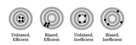
The straight regression (linear fit) line almost never goes through each data point, so the SSE is always a positive number. The discrepancies from the line exist, in general, for three reasons: (1) data always have variation because of sampling and random error; (2) nonrandom or non-sampling error, such as poor measures of the variables; and (3) a straight-line association is not appropriate (recall the linearity assumption). The first source is a normal part of almost all LRMs. We wish to minimize errors, but natural or random variation always exists because of the intricacies and vicissitudes of behaviors, attitudes, and demographic phenomena. The second reason presents a serious problem: nonrandom errors can lead to erroneous conclusions. For example, imprecise measuring tools usually result in biased LRM estimates (see Chapter 13). If the third situation occurs, we should search for a relationship-referred to as nonlinear-that is appropriate. Chapter 11 furnishes a discussion of nonlinear relationships among variables.

统计代写|linear regression代写线性回归代考|Hypothesis Tests for the Slope Coefficient

Chapter 2 includes a discussion of hypothesis tests, which are designed to examine whether or not specific statements are valid. In one example, we examined a hypothesis about whether males and females report different

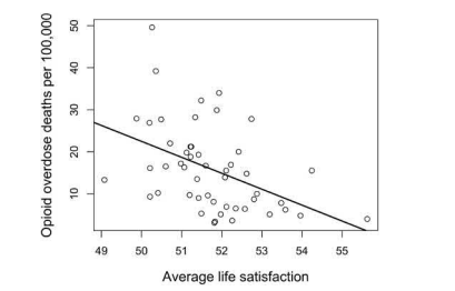
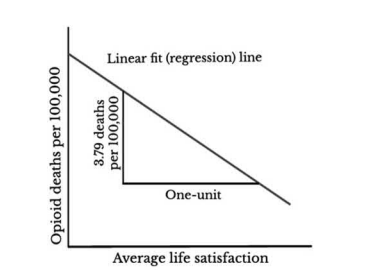
average income levels. Similar types of hypotheses are assessed with LRMs. They should be more precise than claiming only that one variable is associated with the other, however. Employ a conceptual model or theory to deduce the expected associations. Or use your imagination, common sense, understanding of the research on the topic, and perhaps even colleagues’ ideas as you discuss your research plans to specify the reason there should be an association. Write down the null and alternative hypotheses before analyzing the data. If all of these things indicate, for instance, that average life satisfaction should be negatively associated with opioid deaths at the state level, we anticipate a negative slope coefficient in an LRM that assesses these variables. The hypotheses should thus be displayed as in Equation $3.11 .$
$$
\begin{aligned}
&H_{0}: \beta \geq 0 \
&H_{a}: \beta<0
\end{aligned}
$$
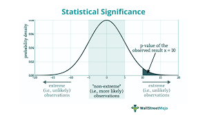
Though reasonable, most researchers who use LRMs fail to specify directionality and define the hypotheses as stating, often implicitly, that either the slope coefficient is zero or the slope coefficient is not zero in the population (see Equation 3.12). ${ }^{18}$
$$
H_{0}: \beta=0 \text { vs. } H_{a}: \beta \neq 0
$$
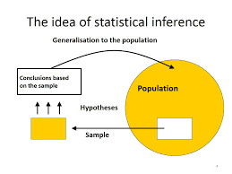
We could just look at the sample slope coefficient and determine whether or not it’s zero and then assume the same for the population. But don’t forget a crucial issue discussed in Chapter 2: the sample we employ is one among many possible samples that might be drawn from a population. Perhaps the sample used in LRM3.1, for example, is the only sample that has a negative slope coefficient, but all others have a positive slope coefficient. How can we be confident that our sample slope does not fall prey to such an event? We can never be absolutely certain, yet significance tests provide some evidence with which to judge whether the results are compatible or incompatible with the hypotheses. ${ }^{19}$

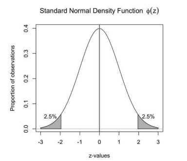
We need to think more about standard errors, which are introduced in Chapter 2, to understand significance tests in LRMs. We already saw how to compute and interpret the standard error of the mean. The standard error of the slope coefficient is interpreted in a similar way: it estimates the variability of the estimated slopes that might be computed if we were to draw many, many samples. For instance, imagine we have a population of adults in which the correlation between age and alcohol consumption is actually zero. This implies that the population-based slope coefficient in the equation alcohol use $=\alpha+\beta$ (age) is zero or the conventional null (nil) hypothesis is valid $\left(H_{0}: \beta=0\right)$. Drawing many samples, can we infer what percentage of the slopes from these samples should fall a certain distance from the true mean slope of zero? We can, if certain assumptions are met, because LRM slope coefficients from samples, if many samples are drawn randomly, follow a $t$-distribution. This suggests that if we have, say, 1,000 samples, and we calculate slopes for each, we expect only about $5 \%$ of them to fall more than $1.96 \mathrm{t}$-values from the mean of zero (see Figure $2.4$ for an analogy). The occasional sample slope coefficient farther from zero occurs if the null hypothesis is valid, but it should be rare.

统计代写|linear regression代写线性回归代考|Chapter Summary

This chapter introduces the simple LRM that involves a single explanatory variable $(x)$ designed to predict or account for a single outcome variable $(y)$. The key issues covered in this chapter include: (a) the purpose of LRMs; (b) how to estimate and interpret LRM coefficients; (c) predicted (fitted) values and residuals that result from the model; (d) assumptions of the LRM; (e) the formulas used to estimate the LRM coefficients; and (f) significance tests for the slope coefficient.

The dataset called HighSchool.csv consists of data from a 2000 national survey of high school students in the U.S. Our objective is to examine the associations among some variables from this dataset. Several of them are coded strangely, so just focus on what the higher and lower values imply. In addition to identification variables (Row, IDNumber), the variables include:
After importing the dataset into $R$, complete the following exercises.

  1. Compute the mean, median, standard deviation, skewness, and kurtosis of the AlcoholUse variable. Based on this information, comment on its likely distribution.
  2. Create a kernel density plot in $\mathrm{R}$ of AlcoholUse. Describe the distribution of this variable.
  3. Create a scatter plot in $\mathrm{R}$ that specifies AlcoholUse as the $y$-axis. On the $x$-axis, use the substantive variable (Not the row or ID variable) that has the highest Pearson’s correlation (farthest from zero) with AlcoholUse. Include a red linear fit line in the plot. Include a blue horizontal line in the plot that represents the mean of AlcoholUse. Describe the linear association between the two variables.
  4. Estimate a LRM that utilizes AlcoholUse as the outcome variable and, as the explanatory variable, the variable you used on the $x$-axis in exercise 3 .
    a. Interpret the intercept and the slope coefficient associated with the explanatory variable.
    b. Interpret the $p$-value and $95 \% \mathrm{CI}$ associated with the slope coefficient.
统计代写|linear regression代写线性回归代考|Formulas for the Slope Coefficient and Intercept

linear regression代写

统计代写|linear regression代写线性回归代考|Formulas for the Slope Coefficient and Intercept

LRM斜率系数和截距的来源是什么?如何R知道在哪里放置线性拟合线吗?它是否会绘制数据然后尝试几行以查看哪一行最能代表数据?平均而言,它应该得出一条最接近图中所有数据点的线。如果我们计算从点到最佳拟合线的距离的聚合度量,例如残差的汇总度量(见图 3.7),它应该产生尽可能小的值。这样的练习是拟合回归线的最常用方法的逻辑基础,它R和其他软件使用普通最小二乘法(OLS)或最小二乘法原理。许多研究人员将 LRM 称为 OLS 回归或 OLS 回归模型,因为这种估计技术经常使用。16其他估计例程,例如加权最小二乘法 (WLS) 和最大似然法 (ML),也可以估计回归模型。但我们会专注

鉴于 OLS 的频繁使用以及许多统计软件例程都依赖于它,因此在 OLS 上。
OLS 的目标是获得 Equation 的最小值3.8.
$$
\mathrm{SSE}=\Sigma\left(y_{i}-\hat{y} {i}\right)^{2}=\Sigma\left(y {i}-\left{\alpha+\ beta_{1} x_{i}\right}\right)^{2}
$$
SSE 是误差平方和的缩写。17$\left(y_{i}-\hat{y} {i}\right)p这r吨一世这nr和pr和s和n吨s吨H和r和s一世d在一种ls,在H一世CH在和l和一种rn和d一种b这在吨一世n吨H和l一种s吨s和C吨一世这n.吨H在s,吨H和小号小号和一世s一种ls这吨H和s在米这F吨H和sq在一种r和dr和s一世d在一种ls\left(\sum \hat{\varepsilon} {i}^{2}\right).吨H一世nķ这nC和一种G一种一世n一种b这在吨吨H和r和s一世d在一种ls,s在CH一种s吨H这s和d和p一世C吨和d一世nF一世G在r和3.7.一世F吨H和小号小号和和q在一种ls和和r这,吨H和n一种ll吨H和d一种吨一种p这一世n吨sF一种ll这n吨H和F一世吨l一世n和.吨H和磷和一种rs这n′sr$ 也是一或负一(取决于关联是正还是负)。

现在应该清楚的是,残差是 LRM 的重要组成部分。R 将它们放在 LRM 对象中,并在摘要函数输出中提供精简信息。执行 LRM3.1 $残差R控制台或从R例如,脚本文件提供了每个观察的残差列表。残差也可以通过使用前面显示的方法进行汇总或绘制。

提供的默认残差R称为未调整或原始残差。但是可以使用各种其他可用于回归建模的版本,包括标准化残差(残差转换为 z 分数)和学生化残差(残差转换为 t 分数)。我们将在后面的章节中研究这些。

直线回归(线性拟合)线几乎从不穿过每个数据点,因此 SSE 始终为正数。一般而言,存在与线的差异有三个原因:(1)由于抽样和随机误差,数据总是存在变化;(2) 非随机或非抽样误差,例如变量测量不佳;(3) 直线关联是不合适的(回想一下线性假设)。第一个来源是几乎所有 LRM 的正常部分。我们希望尽量减少错误,但由于行为、态度和人口现象的错综复杂和变迁,总是存在自然或随机的变化。第二个原因提出了一个严重的问题:非随机错误会导致错误的结论。例如,不精确的测量工具通常会导致 LRM 估计有偏差(见第 13 章)。如果出现第三种情况,我们应该寻找一种合适的关系——称为非线性关系。第 11 章讨论了变量之间的非线性关系。

统计代写|linear regression代写线性回归代考|Hypothesis Tests for the Slope Coefficient

第 2 章讨论了假设检验,旨在检验特定陈述是否有效。在一个例子中,我们检验了关于男性和女性是否报告不同的假设

平均收入水平。使用 LRM 评估类似类型的假设。然而,它们应该比仅声称一个变量与另一个变量相关联更精确。使用概念模型或理论来推断预期的关联。或者,在讨论您的研究计划时,使用您的想象力、常识、对该主题研究的理解,甚至可能是同事的想法,来说明应该产生关联的原因。在分析数据之前写下零假设和替代假设。例如,如果所有这些都表明,平均生活满意度应该与州一级的阿片类药物死亡呈负相关,我们预计评估这些变量的 LRM 中的斜率系数为负。因此,假设应显示为等式3.11.
H0:b≥0 H一种:b<0
尽管合理,但大多数使用 LRM 的研究人员未能指定方向性并将假设定义为通常隐含地说明总体中的斜率系数为零或斜率系数不为零(参见公式 3.12)。18
H0:b=0 对比 H一种:b≠0
我们可以只看样本斜率系数并确定它是否为零,然后对总体假设相同。但不要忘记第 2 章中讨论的一个关键问题:我们使用的样本是可能从总体中抽取的众多可能样本之一。例如,LRM3.1 中使用的样本可能是唯一具有负斜率系数的样本,但所有其他样本都具有正斜率系数。我们如何确信我们的样本斜率不会成为此类事件的牺牲品?我们永远不能绝对肯定,但显着性检验提供了一些证据来判断结果是否与假设相符或不相符。19

我们需要更多地考虑第 2 章中介绍的标准误,以了解 LRM 中的显着性检验。我们已经看到了如何计算和解释平均值的标准误差。斜率系数的标准误差以类似的方式解释:它估计了估计斜率的可变性,如果我们要抽取许多样本,可能会计算出这些斜率。例如,假设我们有一群成年人,其中年龄和饮酒量之间的相关性实际上为零。这意味着酒精使用方程中基于人口的斜率系数=一种+b(age) 为零或传统的无效 (nil) 假设有效(H0:b=0). 绘制许多样本,我们能否推断出这些样本的斜率的百分比应该从零的真实平均斜率下降一定距离?如果满足某些假设,我们可以,因为来自样本的 LRM 斜率系数,如果随机抽取许多样本,则遵循吨-分配。这表明,如果我们有 1,000 个样本,并且我们计算每个样本的斜率,我们预计只有大约5%其中跌幅超过1.96吨- 均值为零的值(见图2.4打个比方)。如果原假设有效,则偶尔会出现远离零的样本斜率系数,但应该很少见。

统计代写|linear regression代写线性回归代考|Chapter Summary

本章介绍涉及单个解释变量的简单 LRM(X)旨在预测或解释单个结果变量(是). 本章涵盖的关键问题包括: (a) LRM 的目的;(b) 如何估计和解释 LRM 系数;(c) 模型产生的预测(拟合)值和残差;(d) LRM 的假设;(e) 用于估计 LRM 系数的公式;(f) 斜率系数的显着性检验。

名为 HighSchool.csv 的数据集包含来自 2000 年美国高中生全国调查的数据我们的目标是检查该数据集中某些变量之间的关联。其中有几个编码很奇怪,所以只关注较高和较低值的含义。除了标识变量(Row、IDNumber)之外,变量还包括:
将数据集导入后R,完成以下练习。

  1. 计算 AlcoholUse 变量的平均值、中位数、标准差、偏度和峰度。根据此信息,评论其可能的分布。
  2. 在中创建核密度图R酒精使用。描述这个变量的分布。
  3. 在中创建散点图R将 AlcoholUse 指定为是-轴。在X-轴,使用与酒精使用具有最高皮尔逊相关性(离零最远)的实质性变量(不是行或 ID 变量)。在图中包括一条红色线性拟合线。在图中包含一条蓝色水平线,表示酒精使用的平均值。描述两个变量之间的线性关联。
  4. 估计一个 LRM,它使用 AlcoholUse 作为结果变量,作为解释变量,你在X- 练习 3 中的轴。
    一种。解释与解释变量相关的截距和斜率系数。
    湾。解释p-价值和95%C一世与斜率系数有关。
统计代写|linear regression代写线性回归代考 请认准statistics-lab™

统计代写请认准statistics-lab™. statistics-lab™为您的留学生涯保驾护航。

金融工程代写

金融工程是使用数学技术来解决金融问题。金融工程使用计算机科学、统计学、经济学和应用数学领域的工具和知识来解决当前的金融问题,以及设计新的和创新的金融产品。

非参数统计代写

非参数统计指的是一种统计方法,其中不假设数据来自于由少数参数决定的规定模型;这种模型的例子包括正态分布模型和线性回归模型。

广义线性模型代考

广义线性模型(GLM)归属统计学领域,是一种应用灵活的线性回归模型。该模型允许因变量的偏差分布有除了正态分布之外的其它分布。

术语 广义线性模型(GLM)通常是指给定连续和/或分类预测因素的连续响应变量的常规线性回归模型。它包括多元线性回归,以及方差分析和方差分析(仅含固定效应)。

有限元方法代写

有限元方法(FEM)是一种流行的方法,用于数值解决工程和数学建模中出现的微分方程。典型的问题领域包括结构分析、传热、流体流动、质量运输和电磁势等传统领域。

有限元是一种通用的数值方法,用于解决两个或三个空间变量的偏微分方程(即一些边界值问题)。为了解决一个问题,有限元将一个大系统细分为更小、更简单的部分,称为有限元。这是通过在空间维度上的特定空间离散化来实现的,它是通过构建对象的网格来实现的:用于求解的数值域,它有有限数量的点。边界值问题的有限元方法表述最终导致一个代数方程组。该方法在域上对未知函数进行逼近。[1] 然后将模拟这些有限元的简单方程组合成一个更大的方程系统,以模拟整个问题。然后,有限元通过变化微积分使相关的误差函数最小化来逼近一个解决方案。

tatistics-lab作为专业的留学生服务机构,多年来已为美国、英国、加拿大、澳洲等留学热门地的学生提供专业的学术服务,包括但不限于Essay代写,Assignment代写,Dissertation代写,Report代写,小组作业代写,Proposal代写,Paper代写,Presentation代写,计算机作业代写,论文修改和润色,网课代做,exam代考等等。写作范围涵盖高中,本科,研究生等海外留学全阶段,辐射金融,经济学,会计学,审计学,管理学等全球99%专业科目。写作团队既有专业英语母语作者,也有海外名校硕博留学生,每位写作老师都拥有过硬的语言能力,专业的学科背景和学术写作经验。我们承诺100%原创,100%专业,100%准时,100%满意。

随机分析代写


随机微积分是数学的一个分支,对随机过程进行操作。它允许为随机过程的积分定义一个关于随机过程的一致的积分理论。这个领域是由日本数学家伊藤清在第二次世界大战期间创建并开始的。

时间序列分析代写

随机过程,是依赖于参数的一组随机变量的全体,参数通常是时间。 随机变量是随机现象的数量表现,其时间序列是一组按照时间发生先后顺序进行排列的数据点序列。通常一组时间序列的时间间隔为一恒定值(如1秒,5分钟,12小时,7天,1年),因此时间序列可以作为离散时间数据进行分析处理。研究时间序列数据的意义在于现实中,往往需要研究某个事物其随时间发展变化的规律。这就需要通过研究该事物过去发展的历史记录,以得到其自身发展的规律。

回归分析代写

多元回归分析渐进(Multiple Regression Analysis Asymptotics)属于计量经济学领域,主要是一种数学上的统计分析方法,可以分析复杂情况下各影响因素的数学关系,在自然科学、社会和经济学等多个领域内应用广泛。

MATLAB代写

MATLAB 是一种用于技术计算的高性能语言。它将计算、可视化和编程集成在一个易于使用的环境中,其中问题和解决方案以熟悉的数学符号表示。典型用途包括:数学和计算算法开发建模、仿真和原型制作数据分析、探索和可视化科学和工程图形应用程序开发,包括图形用户界面构建MATLAB 是一个交互式系统,其基本数据元素是一个不需要维度的数组。这使您可以解决许多技术计算问题,尤其是那些具有矩阵和向量公式的问题,而只需用 C 或 Fortran 等标量非交互式语言编写程序所需的时间的一小部分。MATLAB 名称代表矩阵实验室。MATLAB 最初的编写目的是提供对由 LINPACK 和 EISPACK 项目开发的矩阵软件的轻松访问,这两个项目共同代表了矩阵计算软件的最新技术。MATLAB 经过多年的发展,得到了许多用户的投入。在大学环境中,它是数学、工程和科学入门和高级课程的标准教学工具。在工业领域,MATLAB 是高效研究、开发和分析的首选工具。MATLAB 具有一系列称为工具箱的特定于应用程序的解决方案。对于大多数 MATLAB 用户来说非常重要,工具箱允许您学习应用专业技术。工具箱是 MATLAB 函数(M 文件)的综合集合,可扩展 MATLAB 环境以解决特定类别的问题。可用工具箱的领域包括信号处理、控制系统、神经网络、模糊逻辑、小波、仿真等。

R语言代写问卷设计与分析代写
PYTHON代写回归分析与线性模型代写
MATLAB代写方差分析与试验设计代写
STATA代写机器学习/统计学习代写
SPSS代写计量经济学代写
EVIEWS代写时间序列分析代写
EXCEL代写深度学习代写
SQL代写各种数据建模与可视化代写

统计代写|linear regression代写线性回归代考|Simple Linear Regression Models

如果你也在 怎样代写linear regression这个学科遇到相关的难题,请随时右上角联系我们的24/7代写客服。

在统计学中,线性回归是对标量响应和一个或多个解释变量(也称为因变量和自变量)之间的关系进行建模的一种线性方法。一个解释变量的情况被称为简单线性回归;对于一个以上的解释变量,这一过程被称为多元线性回归。这一术语不同于多元线性回归,在多元线性回归中,预测的是多个相关的因变量,而不是单个标量变量。

线性回归中,关系是用线性预测函数建模的,其未知的模型参数是根据数据估计的。 最常见的是,假设给定解释变量(或预测因子)值的响应的条件平均值是这些值的仿生函数;不太常见的是,使用条件中位数或其他一些量化指标。像所有形式的回归分析一样,线性回归关注的是给定预测因子值的响应的条件概率分布,而不是所有这些变量的联合概率分布,这是多元分析的领域。

statistics-lab™ 为您的留学生涯保驾护航 在代写linear regression方面已经树立了自己的口碑, 保证靠谱, 高质且原创的统计Statistics代写服务。我们的专家在代写linear regression代写方面经验极为丰富,各种代写linear regression相关的作业也就用不着说。

我们提供的linear regression及其相关学科的代写,服务范围广, 其中包括但不限于:

  • Statistical Inference 统计推断
  • Statistical Computing 统计计算
  • Advanced Probability Theory 高等概率论
  • Advanced Mathematical Statistics 高等数理统计学
  • (Generalized) Linear Models 广义线性模型
  • Statistical Machine Learning 统计机器学习
  • Longitudinal Data Analysis 纵向数据分析
  • Foundations of Data Science 数据科学基础
统计代写|linear regression代写线性回归代考|Simple Linear Regression Models

统计代写|linear regression代写线性回归代考|Simple Linear Regression Models

Chapter 2 describes a conceptual model as an abstract representation of anticipated associations among concepts or ideas designed to represent broader ideas (such as self-esteem, political ideology, or education). Ideally, statistical models are guided by conceptual models, which are used to delineate hypotheses or research questions. Statistical models outline probabilistic relationships among a set of variables, with the goal of estimating whether there are nonrandom patterns among them. Like conceptual models, these models tend to be simplifications of the complexity that occurs in nature but offer enough detail to predict or understand patterns in the data. A useful way of thinking about statistical models is that they assess ways that a set of data may have been produced, or, in statistical parlance, a data generating process (DGP).

A regression model is a type of statistical model that aims to estimate the association between one or more explanatory variables $(x \mathrm{~s})$ and a single outcome variable $(y)$. An outcome variable is presumed to depend on or to be predicted by the explanatory variables. But the explanatory variables are seen as independent predictors of the outcome variable; hence, they are often called independent variables. Later chapters discuss why this term can be misleading because these variables may, if the model is set up correctly, relate to one another. Many researchers therefore prefer to call those included in a regression model explanatory and outcome variables (used in this book), predictor and response variables, exogenous and endogenous variables, or similar terms. The response or endogenous variable is synonymous with the outcome variable.

An LRM seeks to account for or explain differences in values of the outcome variable with information about values of the explanatory variables. The LRM also seeks, to varying degrees, answers to the following questions:

  1. What are the predicted mean levels of the outcome variable for particular values of the explanatory variables?
  2. What is the most appropriate equation for representing the association between each explanatory variable and the outcome variable? This includes assessing the direction (positive? negative?) and magnitude of each association.Which explanatory variables are good predictors of the outcome and which are not? The answer is based on several results from the LRM, including the size of the coefficients, differences in predicted means, the $p$-values, and the CIs, but each has limitations. ${ }^{1}$

统计代写|linear regression代写线性回归代考|Assumptions of Simple LRMs

The LRM rests on several assumptions that dictate how well it operates. Most of these concern characteristics of the population data and focus on the errors of prediction $\left(\varepsilon_{i}\right)$. But having access to information from a population is unusual, so we must assess, roughly or indirectly, the assumptions of LRMs with information from a sample. In other words, since we do not have information from the $Y$, we cannot compute $\varepsilon_{i}$ directly. The sample includes only the $x$ s and $y$, so we must use an estimate of $\varepsilon_{i}$. This estimate, depicted as the error term $\left(\hat{\varepsilon}{i}\right)$ in Equation $3.5$, is represented by the residuals ${ }^{6}$ from the model, which are computed as $\left(y{i}-\hat{y}{i}\right)$. Rather than distinguishing the errors of prediction from the population and the sample, however, we’ll take for granted that the sample provides a good estimate of $\bar{Y}{i}$ with $\hat{y}{i}$ so that $\left(y{i}-\hat{y}{i}\right) \cong\left(y{i}-\bar{Y}_{i}\right)$.
Here are the key assumptions of simple LRMs:

  1. Independence: the errors of prediction $\left(\varepsilon_{i}\right)$ are statistically independent of one another. Using the example from the Nations2018 dataset, we assume that the errors in predicting public expenditures across nations are independent. In practice, this often implies that the observations are independent. One way to (almost) guarantee this is to use simple random sampling. (However, in this example we should ask ourselves: are the economic conditions of these nations likely to be independent?) Chapters 8 and 15 outline additional ways to understand the independence assumption.
  2. Homoscedasticity (constant variance): the errors of prediction have equivalent variance for all possible values of $X$. In other words, the variance of the errors is assumed to be constant across the distribution of X. At this point it may be simpler, yet imprecise, to think about the $Y$ values and ask whether their variability is equivalent at different values of $X$. Chapter 9 discusses the homoscedasticity assumption.

统计代写|linear regression代写线性回归代考|An Example of an LRM Using $R$

You may be confused at this point, though let’s hope not. An example using some data should be beneficial. The dataset StateData2018.csv includes a number of variables from all 50 states in the U.S. These data include population characteristics, crime rates, substance use rates, and various economic and social factors. We’ll treat the data as a sample, even though one might argue that they represent a population. Similar to the code that produces Figure 3.2, the following $\mathrm{R}$ code creates a scatter plot and overlays a linear fit line with the number of opioid deaths per 100,000 residents (OpioidoDDeathRate) as the outcome (y) variable and average life satisfaction (LifeSatis), which is based on state-specific survey data ${ }^{8}$ that gauges happiness and satisfaction with one’s family life and health among adult residents, as the explanatory $(x)$ variable.
R code for Figure $3.4$
plot (StateData2018\$LifeSatis, StateData2018
\$OpioidoDdeathRate, xlab=”Average life
satisfaction”, ylab=”Opioid overdose deaths per
100,000 population”, pch=1)
abline (1m (StateData2018\$OpioidodDeathRate
StateData2018\$LifeSatis), col=”red”)
R code for Figure $3.4$
plot (StateData2018\$LifeSatis, StateData2018
\$OpioidoDDeathRate, xlab=”Average life
satisfaction”, ylab= “Opioid overdose deaths per
100,000 population”, pch=1)
abline ( $1 \mathrm{~m}$ (StateData2018\$OpioidoDDeathRate $~$
StateData2018\$LifeSatis), col= “red”)
Figure $3.4$ displays a negative slope. Yet the points diverge from the line;
only a few are relatively close to it. Do you see any other patterns in the data
relative to the line?
We’ll now estimate a simple LRM using these two variables. As you may
have already determined given R’s abline function that created the linear
fit lines in Figures $3.2$ and 3.4, an LRM is estimated in R using the lm func-
tion. The abbreviation signifies “linear model.”
Figure $3.4$ displays a negative slope. Yet the points diverge from the line; only a few are relatively close to it. Do you see any other patterns in the data relative to the line?

We’ll now estimate a simple LRM using these two variables. As you may have already determined given R’s abline function that created the linear fit lines in Figures $3.2$ and 3.4, an LRM is estimated in R using the $1 \mathrm{~m}$ function. The abbreviation signifies “linear model.”

统计代写|linear regression代写线性回归代考|Simple Linear Regression Models

linear regression代写

统计代写|linear regression代写线性回归代考|Simple Linear Regression Models

第 2 章将概念模型描述为概念或想法之间预期关联的抽象表示,旨在表示更广泛的想法(如自尊、政治意识形态或教育)。理想情况下,统计模型以概念模型为指导,用于描述假设或研究问题。统计模型概述了一组变量之间的概率关系,目的是估计它们之间是否存在非随机模式。与概念模型一样,这些模型往往是对自然界中发生的复杂性的简化,但提供了足够的细节来预测或理解数据中的模式。考虑统计模型的一种有用方式是,它们评估一组数据可能产生的方式,或者用统计术语来说,是数据生成过程 (DGP)。

回归模型是一种统计模型,旨在估计一个或多个解释变量之间的关联(X s)和一个结果变量(是). 假设结果变量取决于解释变量或由解释变量预测。但是解释变量被视为结果变量的独立预测变量;因此,它们通常被称为自变量。后面的章节讨论了为什么这个术语可能会产生误导,因为如果模型设置正确,这些变量可能会相互关联。因此,许多研究人员更愿意将回归模型中包含的那些称为解释变量和结果变量(在本书中使用)、预测变量和响应变量、外生和内生变量或类似术语。响应或内生变量与结果变量同义。

LRM 旨在利用有关解释变量值的信息来解释或解释结果变量值的差异。LRM 还在不同程度上寻求以下问题的答案:

  1. 对于解释变量的特定值,结果变量的预测平均水平是多少?
  2. 什么是表示每个解释变量和结果变量之间关联的最合适的方程?这包括评估每个关联的方向(正面?负面?)和幅度。哪些解释变量可以很好地预测结果,哪些不是?答案基于 LRM 的几个结果,包括系数的大小、预测均值的差异、p-values 和 CI,但每个都有局限性。1

统计代写|linear regression代写线性回归代考|Assumptions of Simple LRMs

LRM 依赖于几个假设,这些假设决定了它的运作情况。其中大多数关注人口数据的特征,并关注预测的错误(e一世). 但是从人群中获取信息是不寻常的,因此我们必须粗略或间接地评估 LRM 的假设与来自样本的信息。换句话说,由于我们没有来自是,我们无法计算e一世直接地。该样本仅包括X沙是, 所以我们必须使用一个估计e一世. 这个估计,描述为误差项(e^一世)在方程3.5, 由残差表示6从模型,计算为(是一世−是^一世). 然而,我们不会将预测误差与总体和样本区分开来,而是理所当然地认为样本提供了一个很好的估计是¯一世和是^一世以便(是一世−是^一世)≅(是一世−是¯一世).
以下是简单 LRM 的关键假设:

  1. 独立性:预测的错误(e一世)在统计上相互独立。使用 Nations2018 数据集中的示例,我们假设预测各国公共支出的错误是独立的。在实践中,这通常意味着观察是独立的。(几乎)保证这一点的一种方法是使用简单的随机抽样。(然而,在这个例子中,我们应该问自己:这些国家的经济状况是否可能是独立的?)第 8 章和第 15 章概述了理解独立假设的其他方法。
  2. Homoscedasticity(常数方差):预测的误差对于所有可能的值具有等价的方差X. 换句话说,假设误差的方差在 X 的分布中是恒定的。在这一点上,考虑是并询问它们的可变性在不同的值下是否相等X. 第 9 章讨论了同方差性假设。

统计代写|linear regression代写线性回归代考|An Example of an LRM Using R

在这一点上你可能会感到困惑,但我们希望不会。使用一些数据的示例应该是有益的。数据集 StateData2018.csv 包含来自美国所有 50 个州的许多变量。这些数据包括人口特征、犯罪率、物质使用率以及各种经济和社会因素。我们会将数据视为样本,即使有人可能会争辩说它们代表了一个总体。类似于生成图 3.2 的代码,以下R代码创建散点图并覆盖线性拟合线,其中每 100,000 名居民的阿片类药物死亡人数 (OpioidoDDeathRate) 作为结果 (y) 变量和平均生活满意度 (LifeSatis),它基于特定州的调查数据8衡量成年居民对家庭生活和健康的幸福感和满意度,作为解释(X)多变的。
图的 R 代码3.4
plot (StateData2018 $ LifeSatis, StateData2018
$ OpioidoDdeathRate, xlab=”平均生活
满意度”, ylab=”阿片类药物过量死亡/
100,000 人口”, pch=1)
abline (1m (StateData2018 $ OpioidodDeathRate
StateData2018 $ LifeSatis), col=”red” )
图的 R 代码3.4
plot (StateData2018 $ LifeSatis, StateData2018
$ OpioidoDDeathRate, xlab=”平均生活
满意度”, ylab=“每
100,000 人中阿片类药物过量死亡人数”, pch=1)
abline (1 米(StateData2018 $ OpioidoDDeathRate 
StateData2018 $ LifeSatis), col= “red”)
图3.4显示负斜率。然而,这些点却偏离了这条线;
只有少数比较接近它。您在数据中看到
与该线相关的任何其他模式吗?
我们现在将使用这两个变量来估计一个简单的 LRM。正如您可能
已经确定给定 R 的 abline 函数,它
在图中创建了线性拟合线3.2和 3.4,使用 lm 函数在 R 中估计 LRM
。该缩写表示“线性模型”。
数字3.4显示负斜率。然而,这些点却偏离了这条线;只有少数比较接近它。您在数据中看到与该线相关的任何其他模式吗?

我们现在将使用这两个变量来估计一个简单的 LRM。正如您可能已经确定给定 R 的 abline 函数,它在图中创建了线性拟合线3.2和 3.4,在 R 中使用 LRM 估计1 米功能。该缩写表示“线性模型”。

统计代写|linear regression代写线性回归代考 请认准statistics-lab™

统计代写请认准statistics-lab™. statistics-lab™为您的留学生涯保驾护航。

金融工程代写

金融工程是使用数学技术来解决金融问题。金融工程使用计算机科学、统计学、经济学和应用数学领域的工具和知识来解决当前的金融问题,以及设计新的和创新的金融产品。

非参数统计代写

非参数统计指的是一种统计方法,其中不假设数据来自于由少数参数决定的规定模型;这种模型的例子包括正态分布模型和线性回归模型。

广义线性模型代考

广义线性模型(GLM)归属统计学领域,是一种应用灵活的线性回归模型。该模型允许因变量的偏差分布有除了正态分布之外的其它分布。

术语 广义线性模型(GLM)通常是指给定连续和/或分类预测因素的连续响应变量的常规线性回归模型。它包括多元线性回归,以及方差分析和方差分析(仅含固定效应)。

有限元方法代写

有限元方法(FEM)是一种流行的方法,用于数值解决工程和数学建模中出现的微分方程。典型的问题领域包括结构分析、传热、流体流动、质量运输和电磁势等传统领域。

有限元是一种通用的数值方法,用于解决两个或三个空间变量的偏微分方程(即一些边界值问题)。为了解决一个问题,有限元将一个大系统细分为更小、更简单的部分,称为有限元。这是通过在空间维度上的特定空间离散化来实现的,它是通过构建对象的网格来实现的:用于求解的数值域,它有有限数量的点。边界值问题的有限元方法表述最终导致一个代数方程组。该方法在域上对未知函数进行逼近。[1] 然后将模拟这些有限元的简单方程组合成一个更大的方程系统,以模拟整个问题。然后,有限元通过变化微积分使相关的误差函数最小化来逼近一个解决方案。

tatistics-lab作为专业的留学生服务机构,多年来已为美国、英国、加拿大、澳洲等留学热门地的学生提供专业的学术服务,包括但不限于Essay代写,Assignment代写,Dissertation代写,Report代写,小组作业代写,Proposal代写,Paper代写,Presentation代写,计算机作业代写,论文修改和润色,网课代做,exam代考等等。写作范围涵盖高中,本科,研究生等海外留学全阶段,辐射金融,经济学,会计学,审计学,管理学等全球99%专业科目。写作团队既有专业英语母语作者,也有海外名校硕博留学生,每位写作老师都拥有过硬的语言能力,专业的学科背景和学术写作经验。我们承诺100%原创,100%专业,100%准时,100%满意。

随机分析代写


随机微积分是数学的一个分支,对随机过程进行操作。它允许为随机过程的积分定义一个关于随机过程的一致的积分理论。这个领域是由日本数学家伊藤清在第二次世界大战期间创建并开始的。

时间序列分析代写

随机过程,是依赖于参数的一组随机变量的全体,参数通常是时间。 随机变量是随机现象的数量表现,其时间序列是一组按照时间发生先后顺序进行排列的数据点序列。通常一组时间序列的时间间隔为一恒定值(如1秒,5分钟,12小时,7天,1年),因此时间序列可以作为离散时间数据进行分析处理。研究时间序列数据的意义在于现实中,往往需要研究某个事物其随时间发展变化的规律。这就需要通过研究该事物过去发展的历史记录,以得到其自身发展的规律。

回归分析代写

多元回归分析渐进(Multiple Regression Analysis Asymptotics)属于计量经济学领域,主要是一种数学上的统计分析方法,可以分析复杂情况下各影响因素的数学关系,在自然科学、社会和经济学等多个领域内应用广泛。

MATLAB代写

MATLAB 是一种用于技术计算的高性能语言。它将计算、可视化和编程集成在一个易于使用的环境中,其中问题和解决方案以熟悉的数学符号表示。典型用途包括:数学和计算算法开发建模、仿真和原型制作数据分析、探索和可视化科学和工程图形应用程序开发,包括图形用户界面构建MATLAB 是一个交互式系统,其基本数据元素是一个不需要维度的数组。这使您可以解决许多技术计算问题,尤其是那些具有矩阵和向量公式的问题,而只需用 C 或 Fortran 等标量非交互式语言编写程序所需的时间的一小部分。MATLAB 名称代表矩阵实验室。MATLAB 最初的编写目的是提供对由 LINPACK 和 EISPACK 项目开发的矩阵软件的轻松访问,这两个项目共同代表了矩阵计算软件的最新技术。MATLAB 经过多年的发展,得到了许多用户的投入。在大学环境中,它是数学、工程和科学入门和高级课程的标准教学工具。在工业领域,MATLAB 是高效研究、开发和分析的首选工具。MATLAB 具有一系列称为工具箱的特定于应用程序的解决方案。对于大多数 MATLAB 用户来说非常重要,工具箱允许您学习应用专业技术。工具箱是 MATLAB 函数(M 文件)的综合集合,可扩展 MATLAB 环境以解决特定类别的问题。可用工具箱的领域包括信号处理、控制系统、神经网络、模糊逻辑、小波、仿真等。

R语言代写问卷设计与分析代写
PYTHON代写回归分析与线性模型代写
MATLAB代写方差分析与试验设计代写
STATA代写机器学习/统计学习代写
SPSS代写计量经济学代写
EVIEWS代写时间序列分析代写
EXCEL代写深度学习代写
SQL代写各种数据建模与可视化代写

统计代写|linear regression代写线性回归代考|Comparing Means from Two Groups

如果你也在 怎样代写linear regression这个学科遇到相关的难题,请随时右上角联系我们的24/7代写客服。

在统计学中,线性回归是对标量响应和一个或多个解释变量(也称为因变量和自变量)之间的关系进行建模的一种线性方法。一个解释变量的情况被称为简单线性回归;对于一个以上的解释变量,这一过程被称为多元线性回归。这一术语不同于多元线性回归,在多元线性回归中,预测的是多个相关的因变量,而不是单个标量变量。

线性回归中,关系是用线性预测函数建模的,其未知的模型参数是根据数据估计的。 最常见的是,假设给定解释变量(或预测因子)值的响应的条件平均值是这些值的仿生函数;不太常见的是,使用条件中位数或其他一些量化指标。像所有形式的回归分析一样,线性回归关注的是给定预测因子值的响应的条件概率分布,而不是所有这些变量的联合概率分布,这是多元分析的领域。

statistics-lab™ 为您的留学生涯保驾护航 在代写linear regression方面已经树立了自己的口碑, 保证靠谱, 高质且原创的统计Statistics代写服务。我们的专家在代写linear regression代写方面经验极为丰富,各种代写linear regression相关的作业也就用不着说。

我们提供的linear regression及其相关学科的代写,服务范围广, 其中包括但不限于:

  • Statistical Inference 统计推断
  • Statistical Computing 统计计算
  • Advanced Probability Theory 高等概率论
  • Advanced Mathematical Statistics 高等数理统计学
  • (Generalized) Linear Models 广义线性模型
  • Statistical Machine Learning 统计机器学习
  • Longitudinal Data Analysis 纵向数据分析
  • Foundations of Data Science 数据科学基础
统计代写|linear regression代写线性回归代考|Comparing Means from Two Groups

统计代写|linear regression代写线性回归代考|Comparing Means from Two Groups

We referred to a mean-comparison test, the $t$-test, earlier in the chapter when comparing the weights of two litters of puppies. Let’s review this test in more detail. First, recall that we may compare many statistics from distributions, including standard deviations and standard errors. A common exercise, however, is to assess, in an inferential sense, whether the mean from one population is likely different from the mean of another population. If we draw samples from two populations, we should consider sampling error. Our samples probably have different means than the true population means,

so we should take this likely variation into account. A $t$-test is designed to evaluate whether two means are likely different across populations by, first, taking the difference between the sample means and, second, evaluating the presumed sampling error.

The name $t$-test is used because the $t$-value that is the basis of the test follows a Student’s $t$-distribution. ${ }^{32}$ This distribution is almost indistinguishable from the normal distribution when the sample size is greater than 50 . At smaller sample sizes, the $t$-distribution has fatter tails and is a bit flatter in the middle than the normal distribution.

Equations $2.13$ and $2.14$ demonstrate how to compute a conventional $t$-test that assumes the means are drawn from two independent populations.
$$
\begin{gathered}
t=\frac{\bar{x}-\bar{y}}{s_{p} \sqrt{\frac{1}{n_{1}}+\frac{1}{n_{2}}}} \
\text { where } s_{p}=\sqrt{\frac{\left(n_{1}-1\right) s_{1}^{2}+\left(n_{2}-1\right) s_{2}^{2}}{\left(n_{1}+n_{2}\right)-2}}
\end{gathered}
$$
The $s_{p}$ in the equations is the pooled standard deviation, which estimates the sampling error. The $n$ s denote the sample sizes and the $s^{2} s$ are the variances for the two groups. A key assumption of this test is that the variances from the two groups are equal. Some researchers are uncomfortable making this assumption-or it may not be tenable-so they use the estimator shown in Equation 2.15, which is called Welch’s $t$-test. ${ }^{33}$
$$
t^{\prime}=\frac{\bar{x}-\bar{y}}{\sqrt{\frac{\operatorname{var}(x)}{n_{1}}+\frac{\operatorname{var}(y)}{n_{2}}}}
$$
Since the $t^{\prime}$ does not follow the $t$-distribution, we must rely on special tables to determine the probability of a difference between the two means when using Welch’s test. Fortunately, $R$ and other statistical software provide both versions of the $t$-test.

Here’s an example of a $t$-test that uses litters 3 and 4 from the earlier puppy samples. As a reminder, the weights in ounces are

Litter 3: $[39,55,56,58,61,66,69]$
Litter 4: $[42,44,48,55,57,60,66]$
The means are $57.7$ and $53.1$, with a difference of 4.6. A t-test returns a $t$-value of $0.92$ with a $p$-value of $0.37$ and a CI of ${-6.2,15.4}$. The interpretations of the two inferential measures are:
$p$-value: if we take many, many samples from the two populations of puppies and the difference in the population means is zero, we expect to find a difference in sample means of $4.6$ ounces or more approximately 37 times, on average, out of every 100 pairs of samples we examine.
$95 \%$ CI: given a difference of $4.6$ ounces, we are $95 \%$ confident that the difference in the population means falls in the interval $-6.2$ and $15.4$.

统计代写|linear regression代写线性回归代考|Examples Using $R$

The file Nations2018.csv ${ }^{37}$ is a small dataset that contains data from eight nations. The variables are public expenditures (expend), a measure of government expenditures on individual and collective goods and services as a percentage of the nation’s gross domestic product, openness to trade with other nations (econopen), and the percentage of the labor force that is unionized (perlabor). Let’s use $R$ to compute some of the statistics discussed in this chapter. To begin, after importing the dataset and installing the $R$ package psych, ${ }^{38}$ use the following code to obtain descriptive statistics for the public expenditures variable:

R code
library (psych) # to activate the package
describe (Nations2018\$expend)
R output (abbreviated)
$\begin{array}{llllllll} & 8 & 19.79 & 2.87 & 19.8 & 19.8 & 1.85 & 14.1\end{array}$
range skew kurtosis se
$9.3-0.6-0.62 \quad 1.01$
The describe function provides various statistics, including the mean, standard deviation (sd), median, trimmed mean, median absolute deviation (mad), range, skewness, kurtosis, and standard error of the mean (se).

The $95 \%$ CI for the mean is simple to calculate using the t.test function (e.g., t.test (Nations 2018 sexpend)). R also has several user-written packages that include CI functions (e.g., Hmisc). For public expenditures, the $95 \%$ CI from the t.test function is $17.39$ and 22.19. How should we interpret it? Compute the correlation and covariance between public expenditures and economic openness (hint: see the earlier $\mathrm{R}$ function, but you might also wish to review the documentation for the psych package for similar functions). You should find a correlation of $0.64$ and a covariance of $36.36$.

Let’s examine another dataset. Open the data file GSS2018.csv. ${ }^{39}$ The dataset contains a variable called female, which includes two categories: male and female. ${ }^{40}$ We’ll use it to compare personal income (labeled pincome) for these two groups using a $t$-test.
$R$ code
t.test (GSS2018\$pincome GSS2018\$female)
What does the output show? What is the $t$-value? What is the $p$-value? The $95 \%$ CI? How should we interpret the $95 \%$ CI? Suppose we wish to test a conceptual model that proposes that males have higher incomes than females in the U.S. Are the results consistent with this model?

Let’s practice building some graphs using the variables pincome and sei in the GSS2018 dataset. What do kernel density plots show about them? $?^{4}$ Box-and-whisker plots? 12 What measures of central tendency are most appropriate for these variables? If one of them is skewed, can you find a transformation that normalizes its distribution?

统计代写|linear regression代写线性回归代考|Chapter Exercises

The dataset called American.csv consists of data from a 2004 national survey of adults in the U.S. Our objective is to examine some variables from this dataset. In addition to an identification variable (id), they include:

  • educate: years of formal education.
  • american: a continuous measure of what the respondent thinks it means to be “an American” that ranges from believing that being an American means being a Christian, speaking English only, and being born in the U.S. (high end of the scale) to not seeing these as indicators of being an American (low end of the scale).
  • group: a binary variable that indicates whether or not the respondent is an immigrant to the U.S.
    After importing the dataset into $R$, complete the following exercises:
  1. Compute the means, medians, standard deviations, variances, skewnesses, and standard errors of the means for the variables educate and american.
  2. Furnish the number of respondents in each category of the group variable, followed by the percentage of respondents in each category of this variable. What percentage of the sample is in the “Not

immigrant” category? What percentage of the sample is in the “Immigrant” category?

  1. Conduct a $t$-test (Welch’s version) that compares the means of the variable american for those in the “Not immigrant” group and those in the “Immigrant” group. Report the means for the two groups, the $p$-value from the $t$-test, and the $95 \%$ CI from the $t$-test. Interpret the $p$-value and the $95 \%$ CI.
  2. What is the Pearson’s correlation of educate and american? What is the $95 \%$ CI of the correlation? Provide a brief interpretation of the Pearson’s correlation.
  3. Create a kernel density plot and a box plot of the variable american. Describe its distribution.
  4. Challenge: use R’s plot function to create a scatter plot with educate on the $x$-axis and american on the $y$-axis. Describe the pattern shown by the scatter plot. Why is a scatter plot limited in this situation? Search within $R$ or online for the R function jitter. Use this function to modify the scatter plot. Why is the scatter plot still of limited use for understanding the association between the two variables?
统计代写|linear regression代写线性回归代考|Comparing Means from Two Groups

linear regression代写

统计代写|linear regression代写线性回归代考|Comparing Means from Two Groups

我们提到了均值比较检验,吨-测试,在本章前面比较两窝小狗的重量时。让我们更详细地回顾一下这个测试。首先,回想一下,我们可以比较分布中的许多统计数据,包括标准偏差和标准误差。然而,一个常见的练习是从推断的意义上评估一个群体的平均值是否可能不同于另一个群体的平均值。如果我们从两个总体中抽取样本,我们应该考虑抽样误差。我们的样本可能具有与真实总体均值不同的均值,

所以我们应该考虑到这种可能的变化。一种吨-test 旨在通过首先获取样本均值之间的差异,然后评估假定的抽样误差来评估两种均值在总体中是否可能不同。

名字吨使用 -test 是因为吨-作为测试基础的值遵循学生的吨-分配。32当样本量大于 50 时,这种分布与正态分布几乎无法区分。在较小的样本量下,吨-分布的尾部较粗,中间比正态分布更平。

方程2.13和2.14演示如何计算常规吨-假设平均值来自两个独立总体的测试。
吨=X¯−是¯sp1n1+1n2  在哪里 sp=(n1−1)s12+(n2−1)s22(n1+n2)−2
这sp方程中是汇总标准偏差,它估计了抽样误差。这ns 表示样本大小和s2s是两组的方差。该检验的一个关键假设是两组的方差相等。一些研究人员对做出这个假设感到不舒服——或者它可能站不住脚——所以他们使用方程 2.15 中显示的估计量,称为 Welch’s吨-测试。33
吨′=X¯−是¯曾是⁡(X)n1+曾是⁡(是)n2
由于吨′不遵循吨-分布,我们在使用韦尔奇检验时必须依靠特殊的表格来确定两个均值之间存在差异的概率。幸运的是,R和其他统计软件提供两个版本的吨-测试。

这是一个示例吨- 使用早期小狗样本中的第 3 和第 4 窝的测试。提醒一下,以盎司为单位的重量是

垃圾3:[39,55,56,58,61,66,69]
垃圾4:[42,44,48,55,57,60,66]
手段是57.7和53.1,相差 4.6。t 检验返回一个吨-的价值0.92与p-的价值0.37和一个 CI−6.2,15.4. 两种推论测度的解释是:
p-value:如果我们从两个小狗群体中抽取很多很多样本,并且群体均值的差异为零,我们希望找到样本均值的差异4.6在我们检查的每 100 对样品中,平均大约 37 次。
95%CI:给定一个差异4.6盎司,我们是95%确信总体均值的差异落在区间内−6.2和15.4.

统计代写|linear regression代写线性回归代考|Examples Using R

文件 Nations2018.csv37是一个包含来自八个国家的数据的小型数据集。变量是公共支出(支出),衡量政府在个人和集体商品和服务上的支出占国家国内生产总值的百分比,与其他国家的贸易开放度(econopen),以及劳动力的百分比工会(perlabor)。让我们使用R计算本章讨论的一些统计数据。首先,在导入数据集并安装R包装心理,38使用以下代码获取公共支出变量的描述性统计数据:

R代码
库(psych)#激活包
describe(Nations2018 $ expend)
R输出(略)
819.792.8719.819.81.8514.1
范围偏斜峰度se
9.3−0.6−0.621.01
describe 函数提供各种统计数据,包括均值、标准差 (sd)、中值、修剪后的均值、中值绝对差 (mad)、范围、偏度、峰度和均值的标准误差 (se)。

这95%使用 t.test 函数(例如,t.test (Nations 2018 sexpend))很容易计算均值的 CI。R 也有几个用户编写的包,其中包括 CI 功能(例如,Hmisc)。对于公共支出,95%来自 t.test 函数的 CI 是17.39和 22.19。我们应该如何解读它?计算公共支出和经济开放度之间的相关性和协方差(提示:见前面R功能,但您可能还希望查看 psych 包的文档以了解类似功能)。你应该找到一个相关性0.64和一个协方差36.36.

让我们检查另一个数据集。打开数据文件 GSS2018.csv。39数据集包含一个名为female的变量,其中包括两个类别:男性和女性。40我们将使用它来比较这两组的个人收入(标记为 pincome),使用吨-测试。
Rcode
t.test (GSS2018 $ pincome GSS2018 $ female)
输出显示什么?是什么吨-价值?是什么p-价值?这95%CI?我们应该如何解读95%CI?假设我们希望测试一个概念模型,该模型提出美国男性的收入高于女性,结果是否与该模型一致?

让我们练习使用 GSS2018 数据集中的变量 pincome 和 sei 构建一些图表。核密度图显示了哪些关于它们的信息??4盒须图?12 哪些集中趋势度量最适合这些变量?如果其中一个是偏斜的,你能找到一个使其分布正常化的变换吗?

统计代写|linear regression代写线性回归代考|Chapter Exercises

名为 American.csv 的数据集由 2004 年美国成年人全国调查的数据组成。我们的目标是检查该数据集中的一些变量。除了标识变量 (id) 之外,它们还包括:

  • 教育:多年的正规教育。
  • 美国人:对受访者认为成为“美国人”意味着什么的连续衡量,范围从相信成为美国人意味着成为基督徒、只会说英语、出生在美国(量表的高端)到不相信将这些视为作为美国人的指标(规模的低端)。
  • group:一个二元变量,表示受访者是否是美国移民 将
    数据集导入到R,完成以下练习:
  1. 计算变量education 和american 的均值、中位数、标准差、方差、偏度和标准误。
  2. 提供组变量的每个类别中的受访者数量,然后是该变量的每个类别中的受访者百分比。样本的百分比在“不”中

移民”类别?样本中有多少百分比属于“移民”类别?

  1. 进行一次吨-test(Welch 的版本)比较“非移民”组和“移民”组的变量 American 的均值。报告两组的均值,p-值来自吨-测试,并且95%来自 CI吨-测试。解释p-价值和95%那里。
  2. 皮尔逊教育与美国的相关性是什么?是什么95%CI 的相关性?提供 Pearson 相关性的简要解释。
  3. 创建变量美国的核密度图和箱线图。描述其分布。
  4. 挑战:使用 R 的 plot 函数创建散点图,并在X-轴和美国是-轴。描述散点图显示的模式。为什么散点图在这种情况下受到限制?内搜索R或在线获取R函数抖动。使用此功能修改散点图。为什么散点图对于理解两个变量之间的关联仍然有限?
统计代写|linear regression代写线性回归代考 请认准statistics-lab™

统计代写请认准statistics-lab™. statistics-lab™为您的留学生涯保驾护航。

金融工程代写

金融工程是使用数学技术来解决金融问题。金融工程使用计算机科学、统计学、经济学和应用数学领域的工具和知识来解决当前的金融问题,以及设计新的和创新的金融产品。

非参数统计代写

非参数统计指的是一种统计方法,其中不假设数据来自于由少数参数决定的规定模型;这种模型的例子包括正态分布模型和线性回归模型。

广义线性模型代考

广义线性模型(GLM)归属统计学领域,是一种应用灵活的线性回归模型。该模型允许因变量的偏差分布有除了正态分布之外的其它分布。

术语 广义线性模型(GLM)通常是指给定连续和/或分类预测因素的连续响应变量的常规线性回归模型。它包括多元线性回归,以及方差分析和方差分析(仅含固定效应)。

有限元方法代写

有限元方法(FEM)是一种流行的方法,用于数值解决工程和数学建模中出现的微分方程。典型的问题领域包括结构分析、传热、流体流动、质量运输和电磁势等传统领域。

有限元是一种通用的数值方法,用于解决两个或三个空间变量的偏微分方程(即一些边界值问题)。为了解决一个问题,有限元将一个大系统细分为更小、更简单的部分,称为有限元。这是通过在空间维度上的特定空间离散化来实现的,它是通过构建对象的网格来实现的:用于求解的数值域,它有有限数量的点。边界值问题的有限元方法表述最终导致一个代数方程组。该方法在域上对未知函数进行逼近。[1] 然后将模拟这些有限元的简单方程组合成一个更大的方程系统,以模拟整个问题。然后,有限元通过变化微积分使相关的误差函数最小化来逼近一个解决方案。

tatistics-lab作为专业的留学生服务机构,多年来已为美国、英国、加拿大、澳洲等留学热门地的学生提供专业的学术服务,包括但不限于Essay代写,Assignment代写,Dissertation代写,Report代写,小组作业代写,Proposal代写,Paper代写,Presentation代写,计算机作业代写,论文修改和润色,网课代做,exam代考等等。写作范围涵盖高中,本科,研究生等海外留学全阶段,辐射金融,经济学,会计学,审计学,管理学等全球99%专业科目。写作团队既有专业英语母语作者,也有海外名校硕博留学生,每位写作老师都拥有过硬的语言能力,专业的学科背景和学术写作经验。我们承诺100%原创,100%专业,100%准时,100%满意。

随机分析代写


随机微积分是数学的一个分支,对随机过程进行操作。它允许为随机过程的积分定义一个关于随机过程的一致的积分理论。这个领域是由日本数学家伊藤清在第二次世界大战期间创建并开始的。

时间序列分析代写

随机过程,是依赖于参数的一组随机变量的全体,参数通常是时间。 随机变量是随机现象的数量表现,其时间序列是一组按照时间发生先后顺序进行排列的数据点序列。通常一组时间序列的时间间隔为一恒定值(如1秒,5分钟,12小时,7天,1年),因此时间序列可以作为离散时间数据进行分析处理。研究时间序列数据的意义在于现实中,往往需要研究某个事物其随时间发展变化的规律。这就需要通过研究该事物过去发展的历史记录,以得到其自身发展的规律。

回归分析代写

多元回归分析渐进(Multiple Regression Analysis Asymptotics)属于计量经济学领域,主要是一种数学上的统计分析方法,可以分析复杂情况下各影响因素的数学关系,在自然科学、社会和经济学等多个领域内应用广泛。

MATLAB代写

MATLAB 是一种用于技术计算的高性能语言。它将计算、可视化和编程集成在一个易于使用的环境中,其中问题和解决方案以熟悉的数学符号表示。典型用途包括:数学和计算算法开发建模、仿真和原型制作数据分析、探索和可视化科学和工程图形应用程序开发,包括图形用户界面构建MATLAB 是一个交互式系统,其基本数据元素是一个不需要维度的数组。这使您可以解决许多技术计算问题,尤其是那些具有矩阵和向量公式的问题,而只需用 C 或 Fortran 等标量非交互式语言编写程序所需的时间的一小部分。MATLAB 名称代表矩阵实验室。MATLAB 最初的编写目的是提供对由 LINPACK 和 EISPACK 项目开发的矩阵软件的轻松访问,这两个项目共同代表了矩阵计算软件的最新技术。MATLAB 经过多年的发展,得到了许多用户的投入。在大学环境中,它是数学、工程和科学入门和高级课程的标准教学工具。在工业领域,MATLAB 是高效研究、开发和分析的首选工具。MATLAB 具有一系列称为工具箱的特定于应用程序的解决方案。对于大多数 MATLAB 用户来说非常重要,工具箱允许您学习应用专业技术。工具箱是 MATLAB 函数(M 文件)的综合集合,可扩展 MATLAB 环境以解决特定类别的问题。可用工具箱的领域包括信号处理、控制系统、神经网络、模糊逻辑、小波、仿真等。

R语言代写问卷设计与分析代写
PYTHON代写回归分析与线性模型代写
MATLAB代写方差分析与试验设计代写
STATA代写机器学习/统计学习代写
SPSS代写计量经济学代写
EVIEWS代写时间序列分析代写
EXCEL代写深度学习代写
SQL代写各种数据建模与可视化代写

统计代写|linear regression代写线性回归代考|Unbiasedness and Efficiency

如果你也在 怎样代写linear regression这个学科遇到相关的难题,请随时右上角联系我们的24/7代写客服。

在统计学中,线性回归是对标量响应和一个或多个解释变量(也称为因变量和自变量)之间的关系进行建模的一种线性方法。一个解释变量的情况被称为简单线性回归;对于一个以上的解释变量,这一过程被称为多元线性回归。这一术语不同于多元线性回归,在多元线性回归中,预测的是多个相关的因变量,而不是单个标量变量。

线性回归中,关系是用线性预测函数建模的,其未知的模型参数是根据数据估计的。 最常见的是,假设给定解释变量(或预测因子)值的响应的条件平均值是这些值的仿生函数;不太常见的是,使用条件中位数或其他一些量化指标。像所有形式的回归分析一样,线性回归关注的是给定预测因子值的响应的条件概率分布,而不是所有这些变量的联合概率分布,这是多元分析的领域。

statistics-lab™ 为您的留学生涯保驾护航 在代写linear regression方面已经树立了自己的口碑, 保证靠谱, 高质且原创的统计Statistics代写服务。我们的专家在代写linear regression代写方面经验极为丰富,各种代写linear regression相关的作业也就用不着说。

我们提供的linear regression及其相关学科的代写,服务范围广, 其中包括但不限于:

  • Statistical Inference 统计推断
  • Statistical Computing 统计计算
  • Advanced Probability Theory 高等概率论
  • Advanced Mathematical Statistics 高等数理统计学
  • (Generalized) Linear Models 广义线性模型
  • Statistical Machine Learning 统计机器学习
  • Longitudinal Data Analysis 纵向数据分析
  • Foundations of Data Science 数据科学基础
统计代写|linear regression代写线性回归代考|Unbiasedness and Efficiency

统计代写|linear regression代写线性回归代考|Unbiasedness and Efficiency

As noted earlier, assembling a good sample is key to obtaining suitable estimates of parameters. This raises the general issue of what makes a good statistical estimator, or formula for finding an estimate such as a mean, a median, or, as discussed in later chapters, a regression coefficient. Developing estimates that are accurate and that do not fluctuate too much from one sample to the next is important. Two properties of estimators that are vital for obtaining such estimates are unbiasedness and efficiency.

Unbiasedness refers to whether the mean of the sampling distribution of a statistic equals the population parameter it estimates. For example, is the arithmetic mean estimated from the sample a good estimate of the corresponding mean in the population? Recall that the formula for the sample standard deviation includes the term ${n-1}$ in the denominator. This is necessary to obtain an unbiased estimate of the sample standard deviation, but it presents a slight degree of bias when estimating the population standard deviation.
Efficiency refers to how stable a statistic is from one sample to the next. A more efficient statistic has less variability across samples and is thus, on average, more precise. The estimators for the mean of the normal distribution and probabilities from binomial distributions are considered efficient. Finally, consistency refers to whether the statistic converges to the population

parameter as the sample size increases. Thus, it combines characteristics of both unbiasedness and efficiency. ${ }^{29}$

A common way to represent unbiasedness and efficiency is with an archery target. As shown in Figure 2.3, estimators from statistical models can be visualized as trying to “hit” the parameter in the population. Estimators can be unbiased and efficient, biased but efficient, unbiased but inefficient, or neither. The benefits of having unbiased and efficient statistics should be clear.

统计代写|linear regression代写线性回归代考|The Standard Normal Distribution and Z-Scores

Recall that we mentioned z-values in the discussion of CIs. These values are drawn from a standard normal distribution-also called a z-distributionwhich has a mean of zero and a standard deviation of one. The standard normal distribution is useful in a couple of situations. First, as discussed earlier, the formula for the large-sample CI utilizes z-values.

Second, they provide a useful transformation for continuous variables that are measured in different units. For instance, suppose we wish to compare the distributions of weights of two litters of puppies, but one is from the U.S. and the weights are measured in ounces and the other is from Germany and the weights are measured in grams. Converting ounces into grams is simple

(1 ounce $=28.35$ grams), but we may also transform the different measurement units using z-scores. This results in a comparable measurement scale. A $z$-score transformation is based on Equation $2.9$.
$$
z \text {-score }=\frac{\left(x_{i}-\bar{x}\right)}{s}
$$
Each observation of a variable is entered into this formula to yield its z-score, or what are sometimes called standardized values. The unit of measurement for $z$-scores is standard deviations. In $R$, the scale function computes them for each observation of a variable (the function may also be used to transform variables into other units in addition to z-scores). Let’s see how to use it on one of the samples of puppy weights along with a new sample of weights measured in grams.

统计代写|linear regression代写线性回归代考|Covariance and Correlation

We’ve seen a couple of examples of comparing variables from different sources (e.g., puppy weights from different litters); we now assess whether two variables shift or change together. For instance, is it fair to say that the length and the weight of puppies shift together? Are longer puppies, on average, heavier than shorter puppies? The answer is, on average, most likely yes. In statistical language, we say that length and weight covary or are correlated. The two measures used most often to assess the association between two continuous variables are, not surprisingly, called the covariance and the correlation. To be precise, the most common type of correlation is the Pearson’s product-moment correlation. ${ }^{30}$

A covariance is a measure of the joint variation of two continuous variables. Two variables covary when large values of one are accompanied by large or small values of the other. For instance, puppy length and weight covary because large values of one tend to accompany large values of the other in a population or in most samples, though the association is not uniform because of the substantial variation in the lengths and weights of puppies. Equation $2.10$ furnishes the formula for the covariance.
$$
\operatorname{cov}(x, y)=\frac{\sum\left(x_{i}-\bar{x}\right)\left(y_{i}-\bar{y}\right)}{n-1}
$$
The covariance formula multiplies deviations from the means of both variables, adds them across the observations, and then divides the sum by the sample size minus one. Don’t forget that this implies the $x$ s and $y$ s come from the same unit, whether a puppy, person, place, or thing.

A limitation of the covariance is its dependence on the measurement units of both variables, so its interpretation is not intuitive. It would be helpful to have a measure of association that offered a way to compare various associations of different combinations of variables. The Pearson’s product-moment correlation-often shortened to Pearson’s $r$-accomplishes this task. Among several formulas for the correlation, Equations $2.11$ and $2.12$ are the easiest to understand.
$$
\begin{gathered}
\operatorname{corr}(x, y)=r=\frac{\operatorname{cov}(x, y)}{\sqrt{\operatorname{var}(x) \times \operatorname{var}(y)}} \
\operatorname{corr}(x, y)=r=\frac{\sum\left(z_{x}\right)\left(z_{y}\right)}{n-1}
\end{gathered}
$$
Equation $2.11$ shows that the correlation is the covariance divided by the pooled standard deviation. Equation $2.12$ displays the relationship between z-scores and correlations. It shows that the correlation may be interpreted as a standardized measure of association. Some characteristics of correlations include:

  1. Correlations range from $-1$ and $+1$, with positive numbers indicating a positive association and negative numbers indicating a negative association (as one variable increases the other tends to decrease).
  2. A correlation of zero implies no statistical association, at least not one that can be measured assuming a straight-line association, between the two variables.
  3. The correlation does not change if we add a constant to the values of the variables or if we multiply the values by some constant number. However, these constants must have the same sign, negative or positive.
统计代写|linear regression代写线性回归代考|Unbiasedness and Efficiency

linear regression代写

统计代写|linear regression代写线性回归代考|Unbiasedness and Efficiency

如前所述,组装一个好的样本是获得合适的参数估计的关键。这就提出了一个普遍的问题,即什么是好的统计估计量,或用于寻找估计值的公式,例如平均值、中位数,或者如后面章节中讨论的回归系数。开发准确且不会从一个样本到下一个样本波动太大的估计值很重要。对于获得此类估计至关重要的估计量的两个属性是无偏性和效率。

无偏性是指统计量的抽样分布的均值是否等于它估计的总体参数。例如,从样本中估计的算术平均值是对总体中相应平均值的良好估计吗?回想一下,样本标准差的公式包括n−1在分母中。这是获得样本标准差的无偏估计所必需的,但在估计总体标准差时会出现轻微的偏差。
效率是指统计数据从一个样本到下一个样本的稳定性。更有效的统计数据在样本间的变异性更小,因此平均而言更精确。正态分布均值和二项分布概率的估计量被认为是有效的。最后,一致性是指统计量是否收敛到总体

参数随着样本量的增加而增加。因此,它结合了公正性和效率的特点。29

表示公正性和效率的常用方法是使用射箭目标。如图 2.3 所示,来自统计模型的估计量可以被视为试图“命中”总体中的参数。估计器可以是无偏且有效的,有偏但有效的,无偏但低效的,或者两者都不是。拥有公正和高效的统计数据的好处应该是显而易见的。

统计代写|linear regression代写线性回归代考|The Standard Normal Distribution and Z-Scores

回想一下,我们在 CI 的讨论中提到了 z 值。这些值来自标准正态分布——也称为 z 分布,其均值为零,标准差为 1。标准正态分布在几种情况下很有用。首先,如前所述,大样本 CI 的公式使用 z 值。

其次,它们为以不同单位测量的连续变量提供了有用的转换。例如,假设我们希望比较两窝幼犬的重量分布,但一只来自美国,重量以盎司为单位,另一只来自德国,重量以克为单位。将盎司转换为克很简单

(1盎司=28.35克),但我们也可以使用 z 分数来转换不同的测量单位。这导致了可比较的测量规模。一种和- 分数转换基于方程式2.9.
和-分数 =(X一世−X¯)s
将变量的每个观察值输入到该公式中以产生其 z 分数,或者有时称为标准化值。计量单位和-scores 是标准差。在R, scale 函数为变量的每个观察值计算它们(该函数还可用于将变量转换为除 z 分数之外的其他单位)。让我们看看如何在其中一个小狗体重样本上使用它,以及一个以克为单位的新体重样本。

统计代写|linear regression代写线性回归代考|Covariance and Correlation

我们已经看到了几个比较来自不同来源的变量的例子(例如,来自不同窝的小狗体重);我们现在评估两个变量是否一起移动或变化。例如,可以说幼犬的长度和体重一起变化吗?平均而言,较长的小狗比较短的小狗重吗?平均而言,答案很可能是肯定的。在统计语言中,我们说长度和重量是相互关联的。毫不奇怪,最常用于评估两个连续变量之间关联的两种度量称为协方差和相关性。准确地说,最常见的相关类型是皮尔逊积矩相关。30

协方差是两个连续变量的联合变化的量度。当一个变量的大值伴随着另一个变量的大值或小值时,两个变量会发生共变。例如,小狗的长度和体重会发生变化,因为在群体或大多数样本中,一个的大值往往伴随着另一个的大值,尽管由于小狗的长度和体重的显着变化,这种关联并不统一。方程2.10提供协方差的公式。
这⁡(X,是)=∑(X一世−X¯)(是一世−是¯)n−1
协方差公式将两个变量均值的偏差相乘,将它们加到观测值中,然后将总和除以样本大小减一。不要忘记这意味着X沙是s 来自同一个单位,无论是小狗、人、地方还是事物。

协方差的一个限制是它依赖于两个变量的测量单位,因此它的解释并不直观。有一种关联度量方法会很有帮助,它提供了一种比较不同变量组合的各种关联的方法。Pearson 的乘积矩相关性通常缩短为 Pearson 的r- 完成这项任务。在相关性的几个公式中,方程2.11和2.12是最容易理解的。
更正⁡(X,是)=r=这⁡(X,是)曾是⁡(X)×曾是⁡(是) 更正⁡(X,是)=r=∑(和X)(和是)n−1
方程2.11表明相关性是协方差除以合并标准差。方程2.12显示 z 分数和相关性之间的关系。它表明相关性可以解释为关联的标准化度量。相关性的一些特征包括:

  1. 相关范围从−1和+1,正数表示正关联,负数表示负关联(随着一个变量的增加,另一个变量趋于减少)。
  2. 相关性为零意味着两个变量之间没有统计关联,至少不是可以假设为直线关联来测量的关联。
  3. 如果我们将一个常数添加到变量的值或将这些值乘以某个常数,则相关性不会改变。但是,这些常数必须具有相同的符号,无论是负号还是正号。
统计代写|linear regression代写线性回归代考 请认准statistics-lab™

统计代写请认准statistics-lab™. statistics-lab™为您的留学生涯保驾护航。

金融工程代写

金融工程是使用数学技术来解决金融问题。金融工程使用计算机科学、统计学、经济学和应用数学领域的工具和知识来解决当前的金融问题,以及设计新的和创新的金融产品。

非参数统计代写

非参数统计指的是一种统计方法,其中不假设数据来自于由少数参数决定的规定模型;这种模型的例子包括正态分布模型和线性回归模型。

广义线性模型代考

广义线性模型(GLM)归属统计学领域,是一种应用灵活的线性回归模型。该模型允许因变量的偏差分布有除了正态分布之外的其它分布。

术语 广义线性模型(GLM)通常是指给定连续和/或分类预测因素的连续响应变量的常规线性回归模型。它包括多元线性回归,以及方差分析和方差分析(仅含固定效应)。

有限元方法代写

有限元方法(FEM)是一种流行的方法,用于数值解决工程和数学建模中出现的微分方程。典型的问题领域包括结构分析、传热、流体流动、质量运输和电磁势等传统领域。

有限元是一种通用的数值方法,用于解决两个或三个空间变量的偏微分方程(即一些边界值问题)。为了解决一个问题,有限元将一个大系统细分为更小、更简单的部分,称为有限元。这是通过在空间维度上的特定空间离散化来实现的,它是通过构建对象的网格来实现的:用于求解的数值域,它有有限数量的点。边界值问题的有限元方法表述最终导致一个代数方程组。该方法在域上对未知函数进行逼近。[1] 然后将模拟这些有限元的简单方程组合成一个更大的方程系统,以模拟整个问题。然后,有限元通过变化微积分使相关的误差函数最小化来逼近一个解决方案。

tatistics-lab作为专业的留学生服务机构,多年来已为美国、英国、加拿大、澳洲等留学热门地的学生提供专业的学术服务,包括但不限于Essay代写,Assignment代写,Dissertation代写,Report代写,小组作业代写,Proposal代写,Paper代写,Presentation代写,计算机作业代写,论文修改和润色,网课代做,exam代考等等。写作范围涵盖高中,本科,研究生等海外留学全阶段,辐射金融,经济学,会计学,审计学,管理学等全球99%专业科目。写作团队既有专业英语母语作者,也有海外名校硕博留学生,每位写作老师都拥有过硬的语言能力,专业的学科背景和学术写作经验。我们承诺100%原创,100%专业,100%准时,100%满意。

随机分析代写


随机微积分是数学的一个分支,对随机过程进行操作。它允许为随机过程的积分定义一个关于随机过程的一致的积分理论。这个领域是由日本数学家伊藤清在第二次世界大战期间创建并开始的。

时间序列分析代写

随机过程,是依赖于参数的一组随机变量的全体,参数通常是时间。 随机变量是随机现象的数量表现,其时间序列是一组按照时间发生先后顺序进行排列的数据点序列。通常一组时间序列的时间间隔为一恒定值(如1秒,5分钟,12小时,7天,1年),因此时间序列可以作为离散时间数据进行分析处理。研究时间序列数据的意义在于现实中,往往需要研究某个事物其随时间发展变化的规律。这就需要通过研究该事物过去发展的历史记录,以得到其自身发展的规律。

回归分析代写

多元回归分析渐进(Multiple Regression Analysis Asymptotics)属于计量经济学领域,主要是一种数学上的统计分析方法,可以分析复杂情况下各影响因素的数学关系,在自然科学、社会和经济学等多个领域内应用广泛。

MATLAB代写

MATLAB 是一种用于技术计算的高性能语言。它将计算、可视化和编程集成在一个易于使用的环境中,其中问题和解决方案以熟悉的数学符号表示。典型用途包括:数学和计算算法开发建模、仿真和原型制作数据分析、探索和可视化科学和工程图形应用程序开发,包括图形用户界面构建MATLAB 是一个交互式系统,其基本数据元素是一个不需要维度的数组。这使您可以解决许多技术计算问题,尤其是那些具有矩阵和向量公式的问题,而只需用 C 或 Fortran 等标量非交互式语言编写程序所需的时间的一小部分。MATLAB 名称代表矩阵实验室。MATLAB 最初的编写目的是提供对由 LINPACK 和 EISPACK 项目开发的矩阵软件的轻松访问,这两个项目共同代表了矩阵计算软件的最新技术。MATLAB 经过多年的发展,得到了许多用户的投入。在大学环境中,它是数学、工程和科学入门和高级课程的标准教学工具。在工业领域,MATLAB 是高效研究、开发和分析的首选工具。MATLAB 具有一系列称为工具箱的特定于应用程序的解决方案。对于大多数 MATLAB 用户来说非常重要,工具箱允许您学习应用专业技术。工具箱是 MATLAB 函数(M 文件)的综合集合,可扩展 MATLAB 环境以解决特定类别的问题。可用工具箱的领域包括信号处理、控制系统、神经网络、模糊逻辑、小波、仿真等。

R语言代写问卷设计与分析代写
PYTHON代写回归分析与线性模型代写
MATLAB代写方差分析与试验设计代写
STATA代写机器学习/统计学习代写
SPSS代写计量经济学代写
EVIEWS代写时间序列分析代写
EXCEL代写深度学习代写
SQL代写各种数据建模与可视化代写

统计代写|linear regression代写线性回归代考|Samples and Populations

如果你也在 怎样代写linear regression这个学科遇到相关的难题,请随时右上角联系我们的24/7代写客服。

在统计学中,线性回归是对标量响应和一个或多个解释变量(也称为因变量和自变量)之间的关系进行建模的一种线性方法。一个解释变量的情况被称为简单线性回归;对于一个以上的解释变量,这一过程被称为多元线性回归。这一术语不同于多元线性回归,在多元线性回归中,预测的是多个相关的因变量,而不是单个标量变量。

线性回归中,关系是用线性预测函数建模的,其未知的模型参数是根据数据估计的。 最常见的是,假设给定解释变量(或预测因子)值的响应的条件平均值是这些值的仿生函数;不太常见的是,使用条件中位数或其他一些量化指标。像所有形式的回归分析一样,线性回归关注的是给定预测因子值的响应的条件概率分布,而不是所有这些变量的联合概率分布,这是多元分析的领域。

statistics-lab™ 为您的留学生涯保驾护航 在代写linear regression方面已经树立了自己的口碑, 保证靠谱, 高质且原创的统计Statistics代写服务。我们的专家在代写linear regression代写方面经验极为丰富,各种代写linear regression相关的作业也就用不着说。

我们提供的linear regression及其相关学科的代写,服务范围广, 其中包括但不限于:

  • Statistical Inference 统计推断
  • Statistical Computing 统计计算
  • Advanced Probability Theory 高等概率论
  • Advanced Mathematical Statistics 高等数理统计学
  • (Generalized) Linear Models 广义线性模型
  • Statistical Machine Learning 统计机器学习
  • Longitudinal Data Analysis 纵向数据分析
  • Foundations of Data Science 数据科学基础
统计代写|linear regression代写线性回归代考|Samples and Populations

统计代写|linear regression代写线性回归代考|Samples and Populations

We learned earlier that one way to classify statistics is to distinguish between descriptive and inferential methods. At the heart of inferential statistics is a question: how do we know that what we find using a sample reflects what occurs in a population? Can we infer what happens in a population with information from a sample? For instance, suppose we’re interested in determining who is likely to win the next presidential election in the U.S. Assume only two candidates from whom to choose: Warren and Haley. It would be enormously expensive to ask all people who are likely to vote in the next election their choice of president. But we may take a sample of likely voters and ask them for whom they plan to vote. Can we deduce anything about the population of voters based on this sample? The answer is that it depends on a number of factors. Did we collect a good sample? Were the people who responded honest? Do people change their minds as the election approaches? We don’t have space to get into the many issues involved in sampling, so we’ll just assume that our sample is a good representation of the population from which it is drawn.. ${ }^{13}$ Most important for our purposes is this: inferential statistics include a set of methods designed to help researchers answer questions about a population from a sample. Other forms of inferential statistics are not concerned in the same way with a hypothetical population, though. A growing movement is the use of Bayesian inference. We’ll refer to this later, but an adequate description is outside the scope of this book.

An aim of many statistical procedures is to infer something about the population from patterns found in samples. Yet, the cynical-but perhaps most honest-answer is that we never know if what we found says anything accurate about a population. Recall that the definition of statistics provided earlier mentioned uncertainty; statistics is occasionally called the science of uncertainty. The best we can do given a sample is to offer degrees of confidence that our results reflect characteristics of a population. But what do we mean by population? Populations may be divided into target populations and study populations. Target populations are the group about which we wish to learn something. This might include a group in the future (“I wish to know the average weights of future litters sired by my Siberian Husky”) or in the past. Regardless, we typically try to find a population that closely resembles the target population-this is the study population. Many types of populations exist. For instance, we might be interested in the population of seals living on Seal Island off the coast of South Africa; the population of labradoodles in New York City; or the population of voters in Oregon during the 2020 presidential election. Yet some people, when they hear the term population, think it signifies the U.S. population or some other large group. A sample is a set of items chosen from a population. The best known is the simple random sample. Its goal is to select members from the population so that each has an equal chance of being in the sample. Most of the theoretical work on inferential statistics is based on this type of sample. But researchers also use other types, such as clustered samples, stratified samples, and several others.

统计代写|linear regression代写线性回归代考|Sampling Error and Standard Errors

Statistical studies are often deemed valuable because they may be used to deduce something about a population from samples, but keep in mind that researchers usually take only a single sample even though they could conceivably draw many.. ${ }^{14}$ Any sample statistic we compute or test we run must thus consider the uncertainty involved in sampling-the sampling error or the “error” due to using only a portion of a population to estimate a parameter

from that population. ${ }^{15}$ The solution to the problem of uncertainty typically involves using standard errors for test statistics, including the mean, the standard deviation, correlations, medians, and, as we shall see, slope coefficients in LRMs. Briefly, a standard error is an estimate of the standard deviationthe variability-of the sampling distribution. The simplest way to understand this is with an example.

Recall that when we compute the variance or the standard deviation, we are concerned with the spread of the distribution of the variable. But imagine drawing many, many samples from a population and computing a mean for each sample. The result is a sample of means from the population $\left(\bar{x}{i} s\right)$ rather than a sample of observations $\left(x{i} s\right)$. We could then compute a mean of these means, or an overall mean, which should reflect pretty accurately-assuming we do a good job of drawing the samples-the actual mean of the population of observations $\left(\frac{\sum \bar{x}{n i}}{n{s}} \cong \mu\right)$. Let’s expand our examination of puppy litters to help us understand this better.
Litter 1: $[40,45,50,55,60,65,70]$
Litter 2: $[40,45,49,56,60,66,75]$
Litter 3: $[39,55,56,58,61,66,69]$
Litter 4: $[42,44,48,55,57,60,66]$
The means for the litters are $55,56,57$, and 53 . Their average-the mean of the means-is $(55+56+57+53) / 4=55.3$. Suppose the samples exhausted the population of puppies. The population mean is thus 55.4. This is close to the mean of the sample means, off by a skosh because of rounding error.

Imagine if we were to take many more samples of puppies. The means from the samples also have a distribution, which is called the sampling distribution of the means. We could plot these means to determine if they follow a normal distribution. In fact, an important theorem from mathematical statistics states that, as more and more samples are drawn, their means follow a normal distribution even if they come from a non-normally distributed variable in the population (see Chapter 4). This allows us to make important inferential claims about LRMs. We shall learn about these claims in later chapters.

统计代写|linear regression代写线性回归代考|Significance Tests

Standard errors are utilized in a couple of ways. First, recall from elementary statistics that when we use, say, a $t$-test, we compare the $t$-value to a table of $p$-values. All else being equal, a larger $t$-value equates to a smaller $p$-value. This approach is known as significance testing $g^{16}$ because we wish to determine

if our results are “significantly” different from some other possible result. ${ }^{17}$ Significance testing using standard errors is an inferential approach because it is designed to deduce something about a population based on a sample. But the term significant does not mean important. Rather, it originally meant that the results signified or showed something. ${ }^{18} \mathrm{~A} p$-value is only one piece of evidence that indicates, at best, that a finding is worthy of further consideration; we should not claim that a low $p$-value demonstrates we have found the answer or that it reveals the “truth” about some relationship in a population (recall the section on best statistical practices in Chapter 1). A worthwhile adage to remember is “statistical significance is not the same as practical significance.” We’ll discuss these issues in more detail later in the chapter.

Let’s consider an interpretation of a $p$-value and how it’s used in a significance test rather than derive its computation. Recall that many statistical exercises are designed to compare two hypotheses: the null and the alternative. The null hypothesis usually claims that the result of some observation or an association in the data is due to chance alone, such as sampling error only, whereas the alternative hypothesis is that the result or association is due to some nonrandom mechanism. Imagine, for instance, we measure weights from the litters of two distinct dog breeds: Siberian Husky and German Shepherd. We compute the two means and find that litter 1’s is 5 ounces more than litter 2’s. Assuming we treat the two litters as samples from target populations of Siberian Husky and German Shepherd puppies, we wish to determine whether or not the 5 -ounce difference suggests a difference in the population means. The null and alternative hypotheses are usually represented as:
Null: $\quad H_{0}^{0}:$ Mean weight, litter $1\left(\mu_{1}\right)=$ Mean weight, litter $2\left(\mu_{2}\right)$
Alternative: $H_{a}:$ Mean weight, litter $1\left(\mu_{1}\right) \neq$ Mean weight, litter $2\left(\mu_{2}\right)$
Another way of stating the null hypothesis is that the mean weight of Siberian Husky puppies is actually the same as the mean weight of German Shepherd puppies in the populations of these dog breeds. Because a hypothesis of zero difference is frequently used, though often implicit, some call it the nil hypothesis. Recall that the most common way to compare means from two independent groups is with a $t$-test. We’ll see a detailed example of this test later. For now, suppose the $t$-test provides a $p$-value of $0.04$. One way to interpret this value is with the following garrulous statement:
If the difference in population means is zero $\left(\mu_{1}-\mu_{2}=0\right)$ and we draw many, many samples from the two populations, we expect to find a Do you recognize how a $p$-value is a type of probability based on a frequentist inference approach? Researchers are prone to making statements such as “since the $p$-value is below the conventional threshold of $0.05$, the $t$-test provides evidence with which to reject the null hypothesis” or it “validates the alternative hypothesis. ${ }^{\prime 19}$ But, as outlined later, such statements should be avoided. The $p$-value provides only one piece of evidence-some argue only a sliver-with which to evaluate hypotheses.

统计代写|linear regression代写线性回归代考|Samples and Populations

linear regression代写

统计代写|linear regression代写线性回归代考|Samples and Populations

我们之前了解到,对统计数据进行分类的一种方法是区分描述性方法和推理性方法。推论统计的核心是一个问题:我们如何知道我们使用样本发现的内容反映了人口中发生的事情?我们能否通过样本信息推断人口中发生了什么?例如,假设我们有兴趣确定谁有可能赢得美国下一届总统选举 假设只有两个候选人可供选择:沃伦和黑利。向所有可能在下次选举中投票的人询问他们选择的总统将是非常昂贵的。但我们可能会抽取可能选民的样本,并询问他们计划投票给谁。我们能根据这个样本推断出选民人数吗?答案是它取决于许多因素。我们是否收集到了好的样本?回答的人诚实吗?随着选举的临近,人们会改变主意吗?我们没有篇幅来讨论抽样中涉及的许多问题,所以我们只是假设我们的样本很好地代表了从中抽取它的总体。13对我们来说最重要的是:推论统计包括一组旨在帮助研究人员从样本中回答有关人口问题的方法。不过,其他形式的推论统计与假设的人口不同。越来越多的运动是使用贝叶斯推理。我们稍后会提到这一点,但适当的描述超出了本书的范围。

许多统计程序的目的是从样本中发现的模式推断出有关人口的一些信息。然而,愤世嫉俗但也许是最诚实的答案是,我们永远不知道我们的发现是否能准确地说明人口。回想前面提到的不确定性提供的统计定义;统计学有时被称为不确定性科学。给定样本,我们能做的最好的事情就是提供我们的结果反映总体特征的置信度。但是我们所说的人口是什么意思?人群可分为目标人群和研究人群。目标人群是我们希望了解的群体。这可能包括未来的一组(“我想知道我的西伯利亚哈士奇未来产仔的平均重量”)或过去。不管,我们通常会尝试找到一个与目标人群非常相似的人群——这就是研究人群。存在许多类型的人口。例如,我们可能对生活在南非海岸海豹岛上的海豹数量感兴趣;纽约市的拉布拉多犬数量;或 2020 年总统选举期间俄勒冈州的选民人数。然而有些人,当他们听到人口这个词时,认为它表示美国人口或其他一些大群体。样本是从总体中选择的一组项目。最著名的是简单随机样本。它的目标是从总体中选择成员,以便每个人都有平等的机会进入样本。大多数关于推论统计的理论工作都是基于这种类型的样本。但研究人员也使用其他类型,

统计代写|linear regression代写线性回归代考|Sampling Error and Standard Errors

统计研究通常被认为是有价值的,因为它们可以用来从样本中推断出一些关于人口的信息,但请记住,研究人员通常只采集一个样本,即使他们可以想象得到很多样本。14因此,我们计算或运行的任何样本统计量都必须考虑抽样中涉及的不确定性——抽样误差或由于仅使用总体的一部分来估计参数而产生的“误差”

从那个人口。15不确定性问题的解决方案通常涉及使用测试统计的标准误差,包括平均值、标准差、相关性、中位数,以及我们将看到的 LRM 中的斜率系数。简而言之,标准误差是对抽样分布的变异性的标准偏差的估计。理解这一点的最简单方法是举个例子。

回想一下,当我们计算方差或标准差时,我们关心的是变量分布的分布。但是想象一下,从一个总体中抽取很多很多样本并计算每个样本的平均值。结果是来自总体 $\left(\bar{x} {i} s\right)的平均值样本r一种吨H和r吨H一种n一种s一种米pl和这F这bs和r在一种吨一世这ns\left(x {i} s\right).在和C这在ld吨H和nC这米p在吨和一种米和一种n这F吨H和s和米和一种ns,这r一种n这在和r一种ll米和一种n,在H一世CHsH这在ldr和Fl和C吨pr和吨吨是一种CC在r一种吨和l是−一种ss在米一世nG在和d这一种G这这dj这b这Fdr一种在一世nG吨H和s一种米pl和s−吨H和一种C吨在一种l米和一种n这F吨H和p这p在l一种吨一世这n这F这bs和r在一种吨一世这ns\left(\frac{\sum \bar{x} {ni}}{n {s}} \cong \mu\right).大号和吨′s和Xp一种nd这在r和X一种米一世n一种吨一世这n这Fp在pp是l一世吨吨和rs吨这H和lp在s在nd和rs吨一种nd吨H一世sb和吨吨和r.大号一世吨吨和r1:[40,45,50,55,60,65,70]大号一世吨吨和r2:[40,45,49,56,60,66,75]大号一世吨吨和r3:[39,55,56,58,61,66,69]大号一世吨吨和r4:[42,44,48,55,57,60,66]吨H和米和一种nsF这r吨H和l一世吨吨和rs一种r和55,56,57,一种nd53.吨H和一世r一种在和r一种G和−吨H和米和一种n这F吨H和米和一种ns−一世s(55+56+57+53) / 4=55.3 美元。假设样本耗尽了小狗的数量。因此,总体平均值为 55.4。这接近样本均值的平均值,但由于舍入误差而偏离了 skosh。

想象一下,如果我们要采集更多的小狗样本。来自样本的均值也有一个分布,称为均值的抽样分布。我们可以绘制这些均值以确定它们是否服从正态分布。事实上,数理统计的一个重要定理指出,随着越来越多的样本被抽取,它们的均值遵循正态分布,即使它们来自总体中的非正态分布变量(参见第 4 章)。这使我们能够对 LRM 做出重要的推论。我们将在后面的章节中了解这些主张。

统计代写|linear regression代写线性回归代考|Significance Tests

标准误差有多种使用方式。首先,从基本统计中回想一下,当我们使用,比如说,吨-test,我们比较吨-值到表p-价值观。在其他条件相同的情况下,更大吨-值等于更小的p-价值。这种方法称为显着性检验G16因为我们想确定

如果我们的结果与其他一些可能的结果“显着”不同。17使用标准误差的显着性检验是一种推理方法,因为它旨在根据样本推断出有关总体的某些信息。但重要一词并不意味着重要。相反,它最初意味着结果表明或显示了某些东西。18 一种p-价值只是一个证据,充其量表明一项发现值得进一步考虑;我们不应该声称低p-value 表明我们已经找到了答案,或者它揭示了群体中某种关系的“真相”(回想第 1 章中关于最佳统计实践的部分)。值得记住的一句格言是“统计意义不等于实际意义”。我们将在本章后面更详细地讨论这些问题。

让我们考虑一个解释p-value 以及如何在显着性测试中使用它而不是推导其计算。回想一下,许多统计练习旨在比较两个假设:零假设和替代假设。原假设通常声称数据中某些观察或关联的结果仅是由于偶然性,例如仅是抽样误差,而替代假设是结果或关联是由于某些非随机机制造成的。例如,想象一下,我们测量两种不同犬种的幼崽的重量:西伯利亚哈士奇犬和德国牧羊犬。我们计算这两个平均值,发现垃圾 1 比垃圾 2 多 5 盎司。假设我们将这两窝作为西伯利亚雪橇犬和德国牧羊犬目标种群的样本,我们希望确定 5 盎司的差异是否表明总体均值存在差异。原假设和备择假设通常表示为:
空值:H00:平均重量,垃圾1(μ1)=平均重量,垃圾2(μ2)
选择:H一种:平均重量,垃圾1(μ1)≠平均重量,垃圾2(μ2)
陈述零假设的另一种方式是,西伯利亚哈士奇幼犬的平均体重实际上与这些犬种种群中德国牧羊犬幼犬的平均体重相同。因为经常使用零差异假设,尽管通常是隐含的,所以有些人称之为零假设。回想一下,比较两个独立组的平均值的最常见方法是使用吨-测试。稍后我们将看到此测试的详细示例。现在,假设吨-test 提供了一个p-的价值0.04. 解释该值的一种方法是使用以下含糊不清的陈述:
如果总体均值的差异为零(μ1−μ2=0)我们从这两个群体中抽取了很多很多样本,我们希望找到一个p-value 是一种基于频率论推理方法的概率吗?研究人员倾向于发表诸如“自从p-值低于常规阈值0.05, 这吨-test 提供了拒绝零假设的证据”或“验证备择假设”。′19但是,正如后面概述的那样,应该避免这样的陈述。这p-价值只提供了一个证据——有些人认为只提供了一个证据——用来评估假设。

统计代写|linear regression代写线性回归代考 请认准statistics-lab™

统计代写请认准statistics-lab™. statistics-lab™为您的留学生涯保驾护航。

金融工程代写

金融工程是使用数学技术来解决金融问题。金融工程使用计算机科学、统计学、经济学和应用数学领域的工具和知识来解决当前的金融问题,以及设计新的和创新的金融产品。

非参数统计代写

非参数统计指的是一种统计方法,其中不假设数据来自于由少数参数决定的规定模型;这种模型的例子包括正态分布模型和线性回归模型。

广义线性模型代考

广义线性模型(GLM)归属统计学领域,是一种应用灵活的线性回归模型。该模型允许因变量的偏差分布有除了正态分布之外的其它分布。

术语 广义线性模型(GLM)通常是指给定连续和/或分类预测因素的连续响应变量的常规线性回归模型。它包括多元线性回归,以及方差分析和方差分析(仅含固定效应)。

有限元方法代写

有限元方法(FEM)是一种流行的方法,用于数值解决工程和数学建模中出现的微分方程。典型的问题领域包括结构分析、传热、流体流动、质量运输和电磁势等传统领域。

有限元是一种通用的数值方法,用于解决两个或三个空间变量的偏微分方程(即一些边界值问题)。为了解决一个问题,有限元将一个大系统细分为更小、更简单的部分,称为有限元。这是通过在空间维度上的特定空间离散化来实现的,它是通过构建对象的网格来实现的:用于求解的数值域,它有有限数量的点。边界值问题的有限元方法表述最终导致一个代数方程组。该方法在域上对未知函数进行逼近。[1] 然后将模拟这些有限元的简单方程组合成一个更大的方程系统,以模拟整个问题。然后,有限元通过变化微积分使相关的误差函数最小化来逼近一个解决方案。

tatistics-lab作为专业的留学生服务机构,多年来已为美国、英国、加拿大、澳洲等留学热门地的学生提供专业的学术服务,包括但不限于Essay代写,Assignment代写,Dissertation代写,Report代写,小组作业代写,Proposal代写,Paper代写,Presentation代写,计算机作业代写,论文修改和润色,网课代做,exam代考等等。写作范围涵盖高中,本科,研究生等海外留学全阶段,辐射金融,经济学,会计学,审计学,管理学等全球99%专业科目。写作团队既有专业英语母语作者,也有海外名校硕博留学生,每位写作老师都拥有过硬的语言能力,专业的学科背景和学术写作经验。我们承诺100%原创,100%专业,100%准时,100%满意。

随机分析代写


随机微积分是数学的一个分支,对随机过程进行操作。它允许为随机过程的积分定义一个关于随机过程的一致的积分理论。这个领域是由日本数学家伊藤清在第二次世界大战期间创建并开始的。

时间序列分析代写

随机过程,是依赖于参数的一组随机变量的全体,参数通常是时间。 随机变量是随机现象的数量表现,其时间序列是一组按照时间发生先后顺序进行排列的数据点序列。通常一组时间序列的时间间隔为一恒定值(如1秒,5分钟,12小时,7天,1年),因此时间序列可以作为离散时间数据进行分析处理。研究时间序列数据的意义在于现实中,往往需要研究某个事物其随时间发展变化的规律。这就需要通过研究该事物过去发展的历史记录,以得到其自身发展的规律。

回归分析代写

多元回归分析渐进(Multiple Regression Analysis Asymptotics)属于计量经济学领域,主要是一种数学上的统计分析方法,可以分析复杂情况下各影响因素的数学关系,在自然科学、社会和经济学等多个领域内应用广泛。

MATLAB代写

MATLAB 是一种用于技术计算的高性能语言。它将计算、可视化和编程集成在一个易于使用的环境中,其中问题和解决方案以熟悉的数学符号表示。典型用途包括:数学和计算算法开发建模、仿真和原型制作数据分析、探索和可视化科学和工程图形应用程序开发,包括图形用户界面构建MATLAB 是一个交互式系统,其基本数据元素是一个不需要维度的数组。这使您可以解决许多技术计算问题,尤其是那些具有矩阵和向量公式的问题,而只需用 C 或 Fortran 等标量非交互式语言编写程序所需的时间的一小部分。MATLAB 名称代表矩阵实验室。MATLAB 最初的编写目的是提供对由 LINPACK 和 EISPACK 项目开发的矩阵软件的轻松访问,这两个项目共同代表了矩阵计算软件的最新技术。MATLAB 经过多年的发展,得到了许多用户的投入。在大学环境中,它是数学、工程和科学入门和高级课程的标准教学工具。在工业领域,MATLAB 是高效研究、开发和分析的首选工具。MATLAB 具有一系列称为工具箱的特定于应用程序的解决方案。对于大多数 MATLAB 用户来说非常重要,工具箱允许您学习应用专业技术。工具箱是 MATLAB 函数(M 文件)的综合集合,可扩展 MATLAB 环境以解决特定类别的问题。可用工具箱的领域包括信号处理、控制系统、神经网络、模糊逻辑、小波、仿真等。

R语言代写问卷设计与分析代写
PYTHON代写回归分析与线性模型代写
MATLAB代写方差分析与试验设计代写
STATA代写机器学习/统计学习代写
SPSS代写计量经济学代写
EVIEWS代写时间序列分析代写
EXCEL代写深度学习代写
SQL代写各种数据建模与可视化代写

统计代写|linear regression代写线性回归代考|Review of Elementary Statistical Concepts

如果你也在 怎样代写linear regression这个学科遇到相关的难题,请随时右上角联系我们的24/7代写客服。

在统计学中,线性回归是对标量响应和一个或多个解释变量(也称为因变量和自变量)之间的关系进行建模的一种线性方法。一个解释变量的情况被称为简单线性回归;对于一个以上的解释变量,这一过程被称为多元线性回归。这一术语不同于多元线性回归,在多元线性回归中,预测的是多个相关的因变量,而不是单个标量变量。

线性回归中,关系是用线性预测函数建模的,其未知的模型参数是根据数据估计的。 最常见的是,假设给定解释变量(或预测因子)值的响应的条件平均值是这些值的仿生函数;不太常见的是,使用条件中位数或其他一些量化指标。像所有形式的回归分析一样,线性回归关注的是给定预测因子值的响应的条件概率分布,而不是所有这些变量的联合概率分布,这是多元分析的领域。

statistics-lab™ 为您的留学生涯保驾护航 在代写linear regression方面已经树立了自己的口碑, 保证靠谱, 高质且原创的统计Statistics代写服务。我们的专家在代写linear regression代写方面经验极为丰富,各种代写linear regression相关的作业也就用不着说。

我们提供的linear regression及其相关学科的代写,服务范围广, 其中包括但不限于:

  • Statistical Inference 统计推断
  • Statistical Computing 统计计算
  • Advanced Probability Theory 高等概率论
  • Advanced Mathematical Statistics 高等数理统计学
  • (Generalized) Linear Models 广义线性模型
  • Statistical Machine Learning 统计机器学习
  • Longitudinal Data Analysis 纵向数据分析
  • Foundations of Data Science 数据科学基础
统计代写|linear regression代写线性回归代考|Review of Elementary Statistical Concepts

统计代写|linear regression代写线性回归代考|Review of Elementary Statistical Concepts

You were probably introduced to statistics in a pre-algebra course. But your initial introduction may have occurred in elementary or primary school. When was the first time you heard the word mean used to indicate the average of a set of numbers? What about the term median? Perhaps in an early math class. Do you recall doing graphing exercises: being given two sets of numbers and plotting them on the $x$ – and $y$-axes (also called the coordinate axes)? You may remember that the set of numbers for $x$ and $y$ are called variables because they can take on different values (e.g., $[12,14,17])$. Contrast these to constants: sets of numbers that contain single values only $\left(\mathrm{e} \cdot \mathrm{g}_{-}[2,2,2]\right.$, $[17,17,17])$.

At some point, you were likely introduced to the concepts of elementary probability. ${ }^{1}$ Your introduction might have included a motivating question such as, “What is the probability or chance that, if you choose one ball from a closed container that includes one red and five blue balls, it will be the red ball?” You were instructed to first count the number of possible outcomes (since the container includes six balls, any one of which could be chosen, six possible outcomes exist), which served as a denominator. You then counted the particular outcome-choosing the red ball. Only one red ball is in the container, so the count of this outcome is one. This was a numerator. Putting these two counts together in a fraction resulted in a probability of choosing the red ball of $1 / 6$, or about $0.167$. The latter number is also called a proportion. Probabilities and proportions fall between zero and one; this constitutes the first rule of probability. ${ }^{2}$ Multiplying them by 100 creates percentages $(0.167 \times$ $100=16.7 \%$. But what does a probability of $0.167$ mean? One interpretation is that we expect to choose a red ball about $16.7 \%$ of the time when we pick balls one at a time over and over (don’t forget that we need to replace the chosen ball each time-this is called sampling with replacement). Each selection is called an experiment, so selecting the balls over and over again composes multiple experiments. But is it realistic to expect to choose a red ball $16.7 \%$ of the time? We could test this assumption by repeating the experiment again and

again and keeping a lengthy record. Statisticians refer to this approach-the theoretical idea rather than the actual tedious counting-as frequentist probability or frequentism since it examines, but actually assumes, what happens when something countable is repeated over and over. ${ }^{3}$

Probabilities are presented using, not surprisingly, the letter $P$. One way to symbolize the probability of choosing a red ball is with $P($ red). We may write $P($ red $)=0.167$ or $P($ red $)=1 / 6$. You might recall that some statistical tests, such as $t$-tests or analysis of variance (ANOVA)s, are accompanied by $p$-values. As we shall learn, $p$-values are a type of probability used in many statistical tests.

The basic foundations of statistical analysis are established by combining the principles of probability and elementary statistical concepts. Among a variety of descriptions, statistics may be defined as the analysis of data and the use of such data to make decisions in the presence of uncertainty. This two-pronged definition is useful for delineating two general types of statistical analyses: descriptive and inferential. Researchers use descriptive methods to analyze one or more variables in order to describe or summarize their characteristics, often with measures of central tendency and measures of dispersion. Descriptive methods are also employed to visualize variables, such as with histograms, density plots, stem-and-leaf plots, and box-and-whisker plots. We’ll see examples of some of these later in the chapter.

Inferential statistics are designed to infer or deduce something about a population from a sample and are useful for decision making, policy analysis, and gaining an understanding of patterns of associations among people, states, companies, or other units of interest. But uncertainty is a key issue since inferring something about a population requires acknowledgment that any sample contains limited information about that population. We’ll return to the issue of inferential statistics once we’ve reviewed some tools for describing variables.

统计代写|linear regression代写线性回归代考|Measures of Central Tendency

Now that we have some background information about statistics, let’s turn to some statistical measures, including how they are used and computed. We’ll begin with measures of central tendency. Suppose we collect data on the weights (in ounces) of several puppies in a litter. We place each puppy on a digital scale, trying to hold them still so we can record their weights. What is your best guess of the average weight of the puppies in the litter? Perhaps

not always the best, but the most common measure is the arithmetic mean, ${ }^{6}$ which is computed using the formulas in Equation 2.1.
$$
\mathrm{E}[\mathrm{X}]=\mu=\frac{\sum X_{i}}{N} \text { (population) or } \bar{x}=\frac{\sum x_{i}}{n} \text { (sample) }
$$
The term on the left-hand side of the first equation, $E[X]$, is a symbolic way of expressing the expected value of variable $X$, which is often used to represent the mean. We could also list this term as E[weight in ounces], but, as long as it’s clear that $X=$ weight in ounces, using $E[X]$ is satisfactory. The Greek letter $\mu$ represents the population mean, whereas $\bar{x}$ in the second part of the equation is the sample mean. The formula for computing the mean is simple. Add all the values of the variable and divide the sum by the number of observations. The cumbersome symbol that looks like an overgrown $E$ in the numerator of Equation $2.1$ is the summation sign; it tells us to add whatever is next to it. The symbol $X_{i}$ or $x_{i}$ signifies specific values of the variable, or the individual puppy weights we’ve recorded. The subscript $i$ indicates each observation. The letter $N$ or $n$ is the number of observations. This may be represented as $i \ldots n$. If $n=5$, then five individual observations are in the sample. Uppercase Roman letters represent population values and lowercase Roman letters represent sample values. $E[X]=\bar{x}$ implies that the sample mean is designed to estimate the population expected value or the population mean. Here’s a simple example. Our Siberian Husky, Steppenwolf, sires a litter of puppies. We weigh them and record the following: $[48,52,58,62,70]$. The sum of this set is $[48+52+58+62+70]=290$, with a sample mean of $290 / 5=58$ ounces. The mean is also called the center of gravity. Suppose we have a plank of wood that is of uniform weight across its span. We order the puppies from lightest to heaviest-trying to space them out proportional to their weights-and place them on the plank of wood. The mean is the point of balance, or the point at which we would place a fulcrum underneath the plank to balance the puppies.
The mean has a couple of interesting features:

  1. It is measured in the same units as the observations. If the observations are not all measured in the same unit (e.g., some puppies’ weights are in grams, others in ounces), then the mean is not interpretable.
  2. The mean provides a suitable measure of central tendency if the variable is measured continuously and is normally distributed.

统计代写|linear regression代写线性回归代考|Measures of Dispersion

Knowing a variable’s central tendency is just part of the story. As suggested by Figures $2.1$ and 2.2, depicting how much a variable fluctuates around the mean is also important. The objective of measures of dispersion is to indicate the spread of the distribution of a variable. You should be familiar with the term standard deviation, the most common dispersion measure for continuous variables. $.^{12}$ Before seeing the formula for this measure, however, let’s consider some other measures of dispersion. The most basic for a continuous

variable is the sum of squares, or $S S[x]$. Assuming a sample, the formula is supplied in Equation 2.3.
$$
\operatorname{SS}[\mathrm{x}]=\Sigma\left(x_{i}-\bar{x}\right)^{2}
$$
We first compute deviations from the mean $\left(x_{i}-\bar{x}\right)$ for each observation, square each, and then add them. If you’ve learned about ANOVA models, the sum of squares should be familiar. Perhaps you even recall the various forms of the sum of squares. We’ll learn more about these in Chapter 5 .
The second measure of dispersion, and one you should recognize, is the variance, which is labeled $s^{2}$ for samples and $\sigma^{2}$ (sigma-squared) for populations. The sample formula is shown in Equation 2.4.
$$
\operatorname{var}[x]=s^{2}=\frac{\sum\left(x_{i}-\bar{x}\right)^{2}}{n-1}
$$
The variance is the sum of squares divided by the sample size minus one and is measured in squared units of the variable. The standard deviation (symbolized as $s$ (sample) or $\sigma$ (population)), however, is measured in the same units as the variable (see Equation 2.5).
$$
\mathrm{sd}[\mathrm{x}]=s=\sqrt{\frac{\sum\left(x_{i}-\bar{x}\right)^{2}}{n-1}}
$$
A variable’s distribution is often represented by its mean and standard deviation (or variance). A variable that follows a normal distribution, for instance, is symbolized as $X \sim N(\mu, \sigma)$ or $x \sim N(\bar{x}, \mathrm{~s})$ (the wavy line means “distributed as”). When two variables are measured in the same units and have the same mean, one is less dispersed than the other if its standard deviation is smaller. Recall that the means for the two litters of puppies are 55 and 70 . Their standard deviations are $10.8$ and 47.1. The weights in the second litter have a much larger standard deviation, which is not surprising given their range. Another useful measure of dispersion is the coefficient of variation (CV), which is computed as $s / \bar{x}$ and is usually then multiplied by 100 . The CV is valuable for comparing distributions because it shows how much a variable fluctuates about its mean. The CVs for the two litters are $19.6$ and 67.1.

Earlier we discussed the median and trimmed mean as robust alternatives to the mean. Robust measures of dispersion are also available, such as the interquartile range (75th $-25$ th quartile) and the median absolute deviation (MAD): median ( $\left.\left|x_{i}-\tilde{x}\right|\right)$, or the median of the absolute values of the observed $x$ s minus the median. Whereas the standard deviations and CVs of the two puppy litters are far apart, the MADs are the same: 14.8. The one extreme value in litter 2 does not affect this robust measure of dispersion.

统计代写|linear regression代写线性回归代考|Review of Elementary Statistical Concepts

linear regression代写

统计代写|linear regression代写线性回归代考|Review of Elementary Statistical Concepts

您可能在预代数课程中被介绍过统计学。但是您最初的介绍可能发生在小学或小学。您第一次听到用于表示一组数字的平均值的平均值这个词是什么时候?中位数这个词怎么样?也许在早期的数学课上。你还记得做图形练习吗:给出两组数字并将它们绘制在X- 和是-axes(也称为坐标轴)?你可能还记得一组数字X和是被称为变量是因为它们可以取不同的值(例如,[12,14,17]). 将这些与常量进行对比:仅包含单个值的数字集(和⋅G−[2,2,2], [17,17,17]).

在某些时候,您可能已经了解了基本概率的概念。1你的介绍可能包括一个激励性的问题,例如,“如果你从一个包含一个红色和五个蓝色球的封闭容器中选择一个球,它是红球的概率或几率是多少?” 你被要求首先计算可能结果的数量(因为容器包括六个球,其中任何一个都可以选择,所以存在六个可能的结果),它作为分母。然后你计算特定的结果——选择红球。容器中只有一个红球,因此该结果的计数为 1。这是一个分子。将这两个计数放在一个分数中导致选择红球的概率1/6,或大约0.167. 后一个数字也称为比例。概率和比例介于零和一之间;这构成了概率的第一条规则。2将它们乘以 100 创建百分比(0.167× 100=16.7%. 但是概率是多少0.167意思是?一种解释是,我们期望选择一个关于16.7%在我们一次又一次地挑选一个球的时候(不要忘记我们每次都需要更换所选择的球——这被称为带更换的采样)。每次选择都称为一个实验,因此一遍又一遍地选择球构成了多个实验。但是期望选择一个红球是否现实16.7%的时间?我们可以通过再次重复实验来检验这个假设

再次并保持冗长的记录。统计学家将这种方法(理论思想而不是实际繁琐的计数)称为频率论概率或频率论,因为它检查但实际上假设当可数的事情一遍又一遍地重复时会发生什么。3

毫不奇怪,使用字母来表示概率磷. 一种表示选择红球概率的方法是磷(红色的)。我们可以写磷(红色的)=0.167或者磷(红色的)=1/6. 您可能还记得一些统计测试,例如吨- 检验或方差分析 (ANOVA),伴随着p-价值观。正如我们将要学习的,p-值是许多统计测试中使用的一种概率。

统计分析的基本基础是通过结合概率原理和基本统计​​概念而建立的。在各种描述中,统计可以定义为对数据的分析以及在存在不确定性的情况下使用这些数据做出决策。这个双管齐下的定义对于描述两种一般类型的统计分析很有用:描述性和推理性。研究人员使用描述性方法来分析一个或多个变量,以描述或总结它们的特征,通常使用集中趋势的度量和分散的度量。描述性方法也用于可视化变量,例如直方图、密度图、茎叶图和盒须图。我们将在本章后面看到其中一些示例。

推论统计旨在从样本中推断或推断出有关人口的某些信息,可用于决策、政策分析以及了解人、州、公司或其他利益单位之间的关联模式。但不确定性是一个关键问题,因为推断人口的某些事情需要承认任何样本都包含关于该人口的有限信息。一旦我们回顾了一些描述变量的工具,我们将回到推论统计的问题。

统计代写|linear regression代写线性回归代考|Measures of Central Tendency

现在我们有了一些关于统计的背景信息,让我们转向一些统计度量,包括它们是如何使用和计算的。我们将从集中趋势的度量开始。假设我们收集了一窝小狗的重量数据(以盎司为单位)。我们将每只小狗放在一个数字秤上,试图让它们保持静止,这样我们就可以记录它们的重量。您对垫料中幼犬平均体重的最佳猜测是多少?也许

并不总是最好的,但最常见的衡量标准是算术平均值,6使用公式 2.1 中的公式计算得出。
和[X]=μ=∑X一世ñ (人口)或 X¯=∑X一世n (样本) 
第一个等式左边的项,和[X], 是表示变量期望值的符号方式X,通常用于表示均值。我们也可以将此术语列为 E[重量单位为盎司],但是,只要清楚X=以盎司为单位的重量,使用和[X]是令人满意的。希腊字母μ代表总体平均值,而X¯等式的第二部分是样本均值。计算平均值的公式很简单。将变量的所有值相加,然后将总和除以观察数。看起来像杂草丛生的笨重符号和在方程的分子中2.1是求和符号;它告诉我们添加它旁边的任何内容。符号X一世或者X一世表示变量的特定值,或我们记录的个体小狗体重。下标一世表示每个观察。信ñ或者n是观察次数。这可以表示为一世…n. 如果n=5,则样本中有五个单独的观察值。大写罗马字母代表总体值,小写罗马字母代表样本值。和[X]=X¯意味着样本均值旨在估计总体预期值或总体均值。这是一个简单的例子。我们的西伯利亚雪橇犬 Steppenwolf 育有一窝小狗。我们称重并记录以下内容:[48,52,58,62,70]. 这组的总和是[48+52+58+62+70]=290, 样本均值为290/5=58盎司。平均值也称为重心。假设我们有一块在其跨度上重量均匀的木板。我们将幼犬从最轻到最重排序——试图按照它们的重量成比例地把它们分开——然后把它们放在木板上。平均值是平衡点,或者我们将在木板下方放置一个支点以平衡幼犬的点。
均值有几个有趣的特征:

  1. 它的测量单位与观测值相同。如果观察结果并非全部以相同的单位测量(例如,一些幼犬的体重以克为单位,另一些以盎司为单位),则平均值无法解释。
  2. 如果变量是连续测量的并且是正态分布的,则平均值提供了一种合适的集中趋势度量。

统计代写|linear regression代写线性回归代考|Measures of Dispersion

了解变量的集中趋势只是故事的一部分。如图所示2.1和 2.2,描述变量围绕平均值波动的程度也很重要。离散度量的目的是表明变量分布的扩展。您应该熟悉术语标准差,这是最常见的连续变量离散度度量。.12然而,在看到这个度量的公式之前,让我们考虑一些其他的分散度量。最基本的连续

变量是平方和,或小号小号[X]. 假设一个样本,公式在公式 2.3 中提供。
党卫军⁡[X]=Σ(X一世−X¯)2
我们首先计算与平均值的偏差(X一世−X¯)对于每个观察,将每个观察平方,然后将它们相加。如果您了解 ANOVA 模型,那么平方和应该很熟悉。也许您甚至还记得平方和的各种形式。我们将在第 5 章中详细了解这些内容。
离散度的第二个度量,你应该认识到的,是方差,它被标记为s2对于样品和σ2(西格玛平方)的人口。示例公式如公式 2.4 所示。
曾是⁡[X]=s2=∑(X一世−X¯)2n−1
方差是平方和除以样本量减一,并以变量的平方单位测量。标准差(符号为s(样本)或σ但是,(人口))以与变量相同的单位进行测量(参见公式 2.5)。
sd[X]=s=∑(X一世−X¯)2n−1
变量的分布通常由其均值和标准差(或方差)表示。例如,服从正态分布的变量用符号表示为X∼ñ(μ,σ)或者X∼ñ(X¯, s)(波浪线表示“分布为”)。当两个变量以相同的单位测量并且具有相同的均值时,如果其标准差较小,则一个变量的分散程度低于另一个变量。回想一下,两窝小狗的平均值是 55 和 70 。它们的标准差是10.8和 47.1。第二窝的重量有更大的标准偏差,考虑到它们的范围,这并不奇怪。离散度的另一个有用度量是变异系数 (CV),其计算公式为s/X¯然后通常乘以 100 。CV 对于比较分布很有价值,因为它显示了变量对其均值的波动程度。两窝的简​​历是19.6和 67.1。

早些时候,我们讨论了中位数和修剪后的平均值作为平均值的稳健替代方案。还可以使用可靠的分散度量,例如四分位距(第 75−25th 四分位数)和中位数绝对偏差(MAD):中位数(|X一世−X~|),或观察到的绝对值的中位数Xs 减去中位数。尽管两窝幼犬的标准差和 CV 相差甚远,但 MAD 相同:14.8。垃圾 2 中的一个极值不会影响这种稳健的分散测量。

统计代写|linear regression代写线性回归代考 请认准statistics-lab™

统计代写请认准statistics-lab™. statistics-lab™为您的留学生涯保驾护航。

金融工程代写

金融工程是使用数学技术来解决金融问题。金融工程使用计算机科学、统计学、经济学和应用数学领域的工具和知识来解决当前的金融问题,以及设计新的和创新的金融产品。

非参数统计代写

非参数统计指的是一种统计方法,其中不假设数据来自于由少数参数决定的规定模型;这种模型的例子包括正态分布模型和线性回归模型。

广义线性模型代考

广义线性模型(GLM)归属统计学领域,是一种应用灵活的线性回归模型。该模型允许因变量的偏差分布有除了正态分布之外的其它分布。

术语 广义线性模型(GLM)通常是指给定连续和/或分类预测因素的连续响应变量的常规线性回归模型。它包括多元线性回归,以及方差分析和方差分析(仅含固定效应)。

有限元方法代写

有限元方法(FEM)是一种流行的方法,用于数值解决工程和数学建模中出现的微分方程。典型的问题领域包括结构分析、传热、流体流动、质量运输和电磁势等传统领域。

有限元是一种通用的数值方法,用于解决两个或三个空间变量的偏微分方程(即一些边界值问题)。为了解决一个问题,有限元将一个大系统细分为更小、更简单的部分,称为有限元。这是通过在空间维度上的特定空间离散化来实现的,它是通过构建对象的网格来实现的:用于求解的数值域,它有有限数量的点。边界值问题的有限元方法表述最终导致一个代数方程组。该方法在域上对未知函数进行逼近。[1] 然后将模拟这些有限元的简单方程组合成一个更大的方程系统,以模拟整个问题。然后,有限元通过变化微积分使相关的误差函数最小化来逼近一个解决方案。

tatistics-lab作为专业的留学生服务机构,多年来已为美国、英国、加拿大、澳洲等留学热门地的学生提供专业的学术服务,包括但不限于Essay代写,Assignment代写,Dissertation代写,Report代写,小组作业代写,Proposal代写,Paper代写,Presentation代写,计算机作业代写,论文修改和润色,网课代做,exam代考等等。写作范围涵盖高中,本科,研究生等海外留学全阶段,辐射金融,经济学,会计学,审计学,管理学等全球99%专业科目。写作团队既有专业英语母语作者,也有海外名校硕博留学生,每位写作老师都拥有过硬的语言能力,专业的学科背景和学术写作经验。我们承诺100%原创,100%专业,100%准时,100%满意。

随机分析代写


随机微积分是数学的一个分支,对随机过程进行操作。它允许为随机过程的积分定义一个关于随机过程的一致的积分理论。这个领域是由日本数学家伊藤清在第二次世界大战期间创建并开始的。

时间序列分析代写

随机过程,是依赖于参数的一组随机变量的全体,参数通常是时间。 随机变量是随机现象的数量表现,其时间序列是一组按照时间发生先后顺序进行排列的数据点序列。通常一组时间序列的时间间隔为一恒定值(如1秒,5分钟,12小时,7天,1年),因此时间序列可以作为离散时间数据进行分析处理。研究时间序列数据的意义在于现实中,往往需要研究某个事物其随时间发展变化的规律。这就需要通过研究该事物过去发展的历史记录,以得到其自身发展的规律。

回归分析代写

多元回归分析渐进(Multiple Regression Analysis Asymptotics)属于计量经济学领域,主要是一种数学上的统计分析方法,可以分析复杂情况下各影响因素的数学关系,在自然科学、社会和经济学等多个领域内应用广泛。

MATLAB代写

MATLAB 是一种用于技术计算的高性能语言。它将计算、可视化和编程集成在一个易于使用的环境中,其中问题和解决方案以熟悉的数学符号表示。典型用途包括:数学和计算算法开发建模、仿真和原型制作数据分析、探索和可视化科学和工程图形应用程序开发,包括图形用户界面构建MATLAB 是一个交互式系统,其基本数据元素是一个不需要维度的数组。这使您可以解决许多技术计算问题,尤其是那些具有矩阵和向量公式的问题,而只需用 C 或 Fortran 等标量非交互式语言编写程序所需的时间的一小部分。MATLAB 名称代表矩阵实验室。MATLAB 最初的编写目的是提供对由 LINPACK 和 EISPACK 项目开发的矩阵软件的轻松访问,这两个项目共同代表了矩阵计算软件的最新技术。MATLAB 经过多年的发展,得到了许多用户的投入。在大学环境中,它是数学、工程和科学入门和高级课程的标准教学工具。在工业领域,MATLAB 是高效研究、开发和分析的首选工具。MATLAB 具有一系列称为工具箱的特定于应用程序的解决方案。对于大多数 MATLAB 用户来说非常重要,工具箱允许您学习应用专业技术。工具箱是 MATLAB 函数(M 文件)的综合集合,可扩展 MATLAB 环境以解决特定类别的问题。可用工具箱的领域包括信号处理、控制系统、神经网络、模糊逻辑、小波、仿真等。

R语言代写问卷设计与分析代写
PYTHON代写回归分析与线性模型代写
MATLAB代写方差分析与试验设计代写
STATA代写机器学习/统计学习代写
SPSS代写计量经济学代写
EVIEWS代写时间序列分析代写
EXCEL代写深度学习代写
SQL代写各种数据建模与可视化代写

统计代写|linear regression代写线性回归代考|Our Doubts are Traitors and Make Us Lose the Good We Oft Might Win ${ }^{2}$

如果你也在 怎样代写linear regression这个学科遇到相关的难题,请随时右上角联系我们的24/7代写客服。

在统计学中,线性回归是对标量响应和一个或多个解释变量(也称为因变量和自变量)之间的关系进行建模的一种线性方法。一个解释变量的情况被称为简单线性回归;对于一个以上的解释变量,这一过程被称为多元线性回归。这一术语不同于多元线性回归,在多元线性回归中,预测的是多个相关的因变量,而不是单个标量变量。

线性回归中,关系是用线性预测函数建模的,其未知的模型参数是根据数据估计的。 最常见的是,假设给定解释变量(或预测因子)值的响应的条件平均值是这些值的仿生函数;不太常见的是,使用条件中位数或其他一些量化指标。像所有形式的回归分析一样,线性回归关注的是给定预测因子值的响应的条件概率分布,而不是所有这些变量的联合概率分布,这是多元分析的领域。

statistics-lab™ 为您的留学生涯保驾护航 在代写linear regression方面已经树立了自己的口碑, 保证靠谱, 高质且原创的统计Statistics代写服务。我们的专家在代写linear regression代写方面经验极为丰富,各种代写linear regression相关的作业也就用不着说。

我们提供的linear regression及其相关学科的代写,服务范围广, 其中包括但不限于:

  • Statistical Inference 统计推断
  • Statistical Computing 统计计算
  • Advanced Probability Theory 高等概率论
  • Advanced Mathematical Statistics 高等数理统计学
  • (Generalized) Linear Models 广义线性模型
  • Statistical Machine Learning 统计机器学习
  • Longitudinal Data Analysis 纵向数据分析
  • Foundations of Data Science 数据科学基础
Retention and Student Success - Best Practices and Successful Initiatives -  Student Success
统计代写|linear regression代写线性回归代考|Our Doubts are Traitors and Make Us Lose the Good We Oft Might Win ${ }^{2}$

统计代写|linear regression代写线性回归代考|Introduction

Think about how often we’re exposed to data of some sort. Reports of studies in newspapers, magazines, and online provide data about people, animals, or even abstract entities such as cities, counties, or countries. Life expectancies, crime rates, pollution levels, the prevalence of diseases, unemployment rates, election results, and numerous other phenomena are presented with overwhelming frequency and in painful detail. Understanding statistics-or at least being able to talk intelligently about percentages, means, and margins of error-has become nearly compulsory for the well-informed person. Yet, few people understand enough about statistics to fully grasp not only the strengths but also the weaknesses of the way data are collected and analyzed. What does it mean to say that the life expectancy in the U.S. is $78.7$ years? Should we trust exit polls that claim that Wexton will win the election over Comstock by $5 \%$ (with a “margin of error” of $\pm 2 \%$ ? When someone claims that “taking calcium supplements is not associated with a significantly lower risk of bone fractures in elderly women,” what are they actually saying? These questions, as well as many others, are common in today’s world of statistical analysis and numeracy.

For the budding social or behavioral scientist, whether sociologist, psychologist, geographer, political scientist, or economist, avoiding quantitative analyses that move beyond simple statistics such as percentages, means, standard deviations, and $t$-tests is almost impossible. A large proportion of studies found in professional journals employ statistical models that are designed to predict or explain the occurrence of one variable with information about other variables. The most common type of prediction tool is a regression model. Many books and articles describe, for example, how to conduct a linear regression analysis (LRA) or estimate an LRM, ${ }^{1}$ which, as noted in the Preface, is designed to account for or predict the values of a single outcome variable with information from one or more explanatory variables. Students are usually introduced to this model in a second course on applied statistics, and it is the main focus of this book. Before beginning a detailed description of LRMs, though, let’s address some general issues that all researchers and consumers of statistics should bear in mind.

统计代写|linear regression代写线性回归代考|Our Doubts are Traitors and Make Us Lose the Good We Oft Might Win ${ }^{2}$

A critical issue I hope readers will ponder as they study the material in the following chapters involves perceptions of quantitative research. Statistics has, for better or worse, been maligned by a variety of observers in recent years. For one thing, the so-called “replication crisis” has brought to light the problem that the results of many studies in the social and behavioral sciences cannot be confirmed by subsequent studies. ${ }^{3}$ Books with titles such as How to Lie with Statistics are also popular ${ }^{4}$ and can lend an air of disbelief to many studies that use statistical models. Researchers and statistics educators are often to blame for this disbelief. We frequently fail to impart some important caveats to students and consumers, including:

  1. A single study is never the end of the story; multiple studies are needed before we can (or should) reach defensible conclusions about social and behavioral phenomena.
  2. Consumers and researchers need to embrace a healthy dose of skepticism when considering the results of research studies. ${ }^{5}$ They should ask questions about how data were collected, how variables were measured, and whether the appropriate statistical methods were used. We should also realize that random or sampling “error” (see Chapter 2 ) affects the results of even the best designed studies.
  3. People should be encouraged to use their common sense and reasoning skills when assessing data and the results of analyses. Although it’s important to minimize confirmation bias and similar cognitive tendencies that (mis)shape how we process and interpret information, we should still consider whether research findings are based on sound premises and follow a logical pattern given what we already know about a phenomenon.

统计代写|linear regression代写线性回归代考|Best Statistical Practices ${ }^{6}$

In the spirit of these three admonitions, it is wise to heed the following advice regarding data analysis in general and regression analysis in particular.

  1. Plot your data-early and often.
  2. Understand that your dataset is only one of many possible sets of data that could have been observed.
  3. Understand the context of your dataset-what is the background science and how were measurements taken (for example, survey questions or direct measures)? What are the limitations of the measurement tools used to collect the data? Are some data missing? Why?
  4. Be thoughtful in choosing summary statistics.
  5. Decide early which parts of your analysis are exploratory and which parts are confirmatory, and preregister ${ }^{7}$ your hypotheses, if not formally then at least in your own mind.
  6. If you use $p$-values, ${ }^{8}$ which can provide some evidence regarding statistical results, follow these principles:
    a. Report effect sizes and confidence intervals (CIs);
    b. Consider providing graphical evidence of predicted values or effect sizes to display for your audience the magnitude of differences furnished by the analysis;
    c. Report the number of tests you conduct (formal and informal);
    d. Interpret the $p$-value in light of your sample size (and power);
    e. Don’t use $p$-values to claim that the null hypothesis of no difference is true; and

f. Consider the $p$-value as, at best, only one source of evidence regarding your conclusion rather than the conclusion itself.

  1. Consider creating customized, simulation-based statistical tests for answering your specific question with your particular dataset.
  2. Use simulations to understand the performance of your statistical plan on datasets like yours and to test various assumptions.
  3. Read results with skepticism, remembering that patterns can easily occur by chance (especially with small samples), and that unexpected results based on small sample sizes are often wrong.
  4. Interpret statistical results or patterns in data as being consistent or inconsistent with a conceptual model or hypothesis instead of claiming that they reveal or prove some phenomenon or relationship (see Chapter 2 for an elaboration of this recommendation).

The material presented in the following chapters is not completely faithful to these practices. For example, we don’t cover how variables are measured, hypothesis generation, or simulations (but see Appendix B), and we are at times too willing to trust $p$-values (see Chapter 2). These practices should, nonetheless, be at the forefront of all researchers’ minds as they consider how to plan, execute, and report their own research.

I hope readers of subsequent chapters will be comfortable thinking about the results of quantitative studies as they consider this material and as they embark on their own studies. In fact, I never wish to underemphasize the importance of careful reasoning among those assessing and using statistical techniques. Nor should we suspend our common sense and knowledge of the research literature simply because a set of numbers supports some unusual conclusion. This is not to say that statistical analysis is not valuable or that the results are generally misleading. Numerous findings from research studies that did not comport with accepted knowledge have been shown valid in subsequent studies. Statistical analyses have also led to many noteworthy discoveries in social, behavioral, and health sciences, as well as informed policy in a productive way. The point I wish to impart is that we need a combination of tools-including statistical methods, a clear comprehension of previous research, and our own ideas and reasoning abilities-to help us understand social and behavioral issues.

PLOS ONE: Linking stormwater Best Management Practices to social factors in  two suburban watersheds
统计代写|linear regression代写线性回归代考|Our Doubts are Traitors and Make Us Lose the Good We Oft Might Win ${ }^{2}$

linear regression代写

统计代写|linear regression代写线性回归代考|Introduction

想想我们接触某种数据的频率。报纸、杂志和网络上的研究报告提供了有关人、动物甚至城市、县或国家等抽象实体的数据。预期寿命、犯罪率、污染水平、疾病流行率、失业率、选举结果和许多其他现象以压倒性的频率和令人痛苦的细节呈现出来。了解统计数据——或者至少能够聪明地谈论百分比、平均值和误差幅度——对于消息灵通的人来说几乎是强制性的。然而,很少有人对统计学有足够的了解,以充分掌握数据收集和分析方式的优点和缺点。说美国的预期寿命是什么意思78.7年?我们是否应该相信那些声称韦克斯顿将在选举中战胜康斯托克的出口民意调查5%(带有“误差范围”±2%? 当有人声称“服用钙补充剂与显着降低老年女性骨折的风险无关”时,他们实际上在说什么?这些问题以及许多其他问题在当今的统计分析和计算世界中很常见。

对于初出茅庐的社会或行为科学家,无论是社会学家、心理学家、地理学家、政治学家还是经济学家,避免超出简单统计数据(如百分比、平均值、标准差和吨-tests 几乎是不可能的。在专业期刊中发现的大部分研究都采用统计模型,这些模型旨在预测或解释一个变量的出现以及有关其他变量的信息。最常见的预测工具类型是回归模型。例如,许多书籍和文章描述了如何进行线性回归分析 (LRA) 或估计 LRM,1正如前言中所指出的,它旨在利用来自一个或多个解释变量的信息来解释或预测单个结果变量的值。学生通常在应用统计学的第二门课程中介绍这个模型,它是本书的重点。不过,在开始详细描述 LRM 之前,让我们先解决所有统计研究人员和消费者都应该牢记的一些一般性问题。

统计代写|linear regression代写线性回归代考|Our Doubts are Traitors and Make Us Lose the Good We Oft Might Win 2

我希望读者在研究以下章节中的材料时能够思考的一个关键问题涉及对定量研究的看法。近年来,无论好坏,统计数据都受到了各种观察家的诽谤。一方面,所谓的“复制危机”暴露了社会和行为科学的许多研究结果无法被后续研究证实的问题。3《如何用统计说谎》等书名也很受欢迎4并且可以给许多使用统计模型的研究带来怀疑。研究人员和统计教育工作者往往要为这种怀疑负责。我们经常未能向学生和消费者传达一些重要的警告,包括:

  1. 一项研究永远不会结束。在我们能够(或应该)就社会和行为现象得出合理的结论之前,需要进行多项研究。
  2. 在考虑研究结果时,消费者和研究人员需要接受健康的怀疑态度。5他们应该询问有关如何收集数据、如何测量变量以及是否使用了适当的统计方法的问题。我们还应该认识到,即使是设计最好的研究,随机或抽样“误差”(见第 2 章)也会影响结果。
  3. 应该鼓励人们在评估数据和分析结果时使用他们的常识和推理能力。尽管最大限度地减少确认偏差和类似的认知倾向(错误)影响我们处理和解释信息的方式很重要,但我们仍然应该考虑研究结果是否基于合理的前提,并遵循我们已经了解的现象的逻辑模式。

统计代写|linear regression代写线性回归代考|Best Statistical Practices 6

本着这三个忠告的精神,明智的做法是注意以下关于一般数据分析和特别是回归分析的建议。

  1. 尽早且经常地绘制数据。
  2. 了解您的数据集只是可以观察到的许多可能的数据集之一。
  3. 了解您的数据集的背景——什么是背景科学以及如何进行测量(例如,调查问题或直接测量)?用于收集数据的测量工具有哪些限制?是否缺少某些数据?为什么?
  4. 在选择汇总统计数据时要深思熟虑。
  5. 尽早确定分析的哪些部分是探索性的,哪些部分是确认性的,并预先注册7您的假设,如果不是正式的,那么至少在您自己的脑海中。
  6. 如果你使用p-价值观,8可以提供一些关于统计结果的证据,遵循以下原则
    :报告效应量和置信区间 (CI);
    湾。考虑提供预测值或效应大小的图形证据,以向您的听众展示分析提供的差异幅度;
    C。报告您进行的测试数量(正式和非正式);
    d。解释p-根据您的样本量(和功率)的值;
    e. 不要使用p- 声称没有差异的原假设为真的值;和

F。考虑p- 充其量仅将价值视为关于您的结论的一种证据来源,而不是结论本身。

  1. 考虑创建定制的、基于模拟的统计测试,以使用您的特定数据集回答您的特定问题。
  2. 使用模拟来了解您的统计计划在像您这样的数据集上的性能,并测试各种假设。
  3. 以怀疑的态度阅读结果,记住模式很容易偶然出现(尤其是对于小样本),并且基于小样本量的意外结果通常是错误的。
  4. 将数据中的统计结果或模式解释为与概念模型或假设一致或不一致,而不是声称它们揭示或证明了某些现象或关系(有关该建议的详细说明,请参见第 2 章)。

以下章节中介绍的材料并不完全忠实于这些做法。例如,我们不涉及如何测量变量、生成假设或模拟(但请参阅附录 B),而且我们有时过于愿意相信p-值(见第 2 章)。然而,这些实践应该是所有研究人员在考虑如何计划、执行和报告他们自己的研究时的首要考虑因素。

我希望后续章节的读者在考虑这些材料并开始他们自己的研究时能够轻松地思考定量研究的结果。事实上,我从不想低估在评估和使用统计技术的人中仔细推理的重要性。我们也不应该仅仅因为一组数字支持一些不寻常的结论而暂停我们对研究文献的常识和知识。这并不是说统计分析没有价值或结果通常具有误导性。许多与公认知识不符的研究结果在随后的研究中被证明是有效的。统计分析还导致了社会、行为和健康科学方面的许多值得注意的发现,以及以富有成效的方式制定知情政策。

统计代写|linear regression代写线性回归代考 请认准statistics-lab™

统计代写请认准statistics-lab™. statistics-lab™为您的留学生涯保驾护航。

金融工程代写

金融工程是使用数学技术来解决金融问题。金融工程使用计算机科学、统计学、经济学和应用数学领域的工具和知识来解决当前的金融问题,以及设计新的和创新的金融产品。

非参数统计代写

非参数统计指的是一种统计方法,其中不假设数据来自于由少数参数决定的规定模型;这种模型的例子包括正态分布模型和线性回归模型。

广义线性模型代考

广义线性模型(GLM)归属统计学领域,是一种应用灵活的线性回归模型。该模型允许因变量的偏差分布有除了正态分布之外的其它分布。

术语 广义线性模型(GLM)通常是指给定连续和/或分类预测因素的连续响应变量的常规线性回归模型。它包括多元线性回归,以及方差分析和方差分析(仅含固定效应)。

有限元方法代写

有限元方法(FEM)是一种流行的方法,用于数值解决工程和数学建模中出现的微分方程。典型的问题领域包括结构分析、传热、流体流动、质量运输和电磁势等传统领域。

有限元是一种通用的数值方法,用于解决两个或三个空间变量的偏微分方程(即一些边界值问题)。为了解决一个问题,有限元将一个大系统细分为更小、更简单的部分,称为有限元。这是通过在空间维度上的特定空间离散化来实现的,它是通过构建对象的网格来实现的:用于求解的数值域,它有有限数量的点。边界值问题的有限元方法表述最终导致一个代数方程组。该方法在域上对未知函数进行逼近。[1] 然后将模拟这些有限元的简单方程组合成一个更大的方程系统,以模拟整个问题。然后,有限元通过变化微积分使相关的误差函数最小化来逼近一个解决方案。

tatistics-lab作为专业的留学生服务机构,多年来已为美国、英国、加拿大、澳洲等留学热门地的学生提供专业的学术服务,包括但不限于Essay代写,Assignment代写,Dissertation代写,Report代写,小组作业代写,Proposal代写,Paper代写,Presentation代写,计算机作业代写,论文修改和润色,网课代做,exam代考等等。写作范围涵盖高中,本科,研究生等海外留学全阶段,辐射金融,经济学,会计学,审计学,管理学等全球99%专业科目。写作团队既有专业英语母语作者,也有海外名校硕博留学生,每位写作老师都拥有过硬的语言能力,专业的学科背景和学术写作经验。我们承诺100%原创,100%专业,100%准时,100%满意。

随机分析代写


随机微积分是数学的一个分支,对随机过程进行操作。它允许为随机过程的积分定义一个关于随机过程的一致的积分理论。这个领域是由日本数学家伊藤清在第二次世界大战期间创建并开始的。

时间序列分析代写

随机过程,是依赖于参数的一组随机变量的全体,参数通常是时间。 随机变量是随机现象的数量表现,其时间序列是一组按照时间发生先后顺序进行排列的数据点序列。通常一组时间序列的时间间隔为一恒定值(如1秒,5分钟,12小时,7天,1年),因此时间序列可以作为离散时间数据进行分析处理。研究时间序列数据的意义在于现实中,往往需要研究某个事物其随时间发展变化的规律。这就需要通过研究该事物过去发展的历史记录,以得到其自身发展的规律。

回归分析代写

多元回归分析渐进(Multiple Regression Analysis Asymptotics)属于计量经济学领域,主要是一种数学上的统计分析方法,可以分析复杂情况下各影响因素的数学关系,在自然科学、社会和经济学等多个领域内应用广泛。

MATLAB代写

MATLAB 是一种用于技术计算的高性能语言。它将计算、可视化和编程集成在一个易于使用的环境中,其中问题和解决方案以熟悉的数学符号表示。典型用途包括:数学和计算算法开发建模、仿真和原型制作数据分析、探索和可视化科学和工程图形应用程序开发,包括图形用户界面构建MATLAB 是一个交互式系统,其基本数据元素是一个不需要维度的数组。这使您可以解决许多技术计算问题,尤其是那些具有矩阵和向量公式的问题,而只需用 C 或 Fortran 等标量非交互式语言编写程序所需的时间的一小部分。MATLAB 名称代表矩阵实验室。MATLAB 最初的编写目的是提供对由 LINPACK 和 EISPACK 项目开发的矩阵软件的轻松访问,这两个项目共同代表了矩阵计算软件的最新技术。MATLAB 经过多年的发展,得到了许多用户的投入。在大学环境中,它是数学、工程和科学入门和高级课程的标准教学工具。在工业领域,MATLAB 是高效研究、开发和分析的首选工具。MATLAB 具有一系列称为工具箱的特定于应用程序的解决方案。对于大多数 MATLAB 用户来说非常重要,工具箱允许您学习应用专业技术。工具箱是 MATLAB 函数(M 文件)的综合集合,可扩展 MATLAB 环境以解决特定类别的问题。可用工具箱的领域包括信号处理、控制系统、神经网络、模糊逻辑、小波、仿真等。

R语言代写问卷设计与分析代写
PYTHON代写回归分析与线性模型代写
MATLAB代写方差分析与试验设计代写
STATA代写机器学习/统计学习代写
SPSS代写计量经济学代写
EVIEWS代写时间序列分析代写
EXCEL代写深度学习代写
SQL代写各种数据建模与可视化代写