分类: 并行计算

计算机代写|并行计算作业代写Parallel Computing代考|CSC267

如果你也在 怎样代写并行计算Parallel Computing这个学科遇到相关的难题,请随时右上角联系我们的24/7代写客服。

并行计算是指将较大的问题分解成较小的、独立的、通常是类似的部分,由通过共享内存通信的多个处理器同时执行的过程,其结果在完成后作为整体算法的一部分被合并。

statistics-lab™ 为您的留学生涯保驾护航 在代写并行计算Parallel Computing方面已经树立了自己的口碑, 保证靠谱, 高质且原创的统计Statistics代写服务。我们的专家在代写并行计算Parallel Computing代写方面经验极为丰富,各种代写并行计算Parallel Computing相关的作业也就用不着说。

我们提供的并行计算Parallel Computing及其相关学科的代写,服务范围广, 其中包括但不限于:

  • Statistical Inference 统计推断
  • Statistical Computing 统计计算
  • Advanced Probability Theory 高等楖率论
  • Advanced Mathematical Statistics 高等数理统计学
  • (Generalized) Linear Models 广义线性模型
  • Statistical Machine Learning 统计机器学习
  • Longitudinal Data Analysis 纵向数据分析
  • Foundations of Data Science 数据科学基础
计算机代写|并行计算作业代写Parallel Computing代考|CSC267

计算机代写|并行计算作业代写Parallel Computing代考|Numerical Versus Analytical Solutions

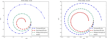
Computers are calculators. If we pass them a certain problem like “here are two bodies interacting through gravity”, they yield values as solution: “the bodies end up at position $\mathrm{x}, \mathrm{y}, \mathrm{z}$ “. They yield numerical solutions. This is different to quite a lot of maths we do in school. There, we manipulate formulae and compute expressions like $F(a, b)=\int_a^b 4 x d x=2 b^2-2 a^2$. Indeed, many teachers save us till the very last minute (or until we have pocket calculators) from inserting actual numbers for $b$ and $a$.

In programming languages, we often speak of variables. But these variables still contain data at any point of the program run. They are fundamentally different to variables in a mathematical formula which might or might not hold specific values. We conclude: There are two different ways to handle equations: We can try to solve them for arbitrary input, i.e. find expressions like $F(a, b)=2 b^2-2 a^2$. Once we have such a solution, we can insert different $a$ and $b$ values. The solution is an analytical solution. ${ }^4$ On a computer, we typically work numerically. We hand in numbers, and we get answers for these particular numbers. But we do not get any universal solution.

Definition $3.2$ (Analytical versus numerical solution) If we solve an equation via formula rewrites such as integration rules, we obtain an analytical solution over the variables. Analytical solutions describe a generic system behaviour. If we solve it for one particular set of initial values right from the start, we strive for a numerical solution.

Computers yield numerical solutions. This statement is not $100 \%$ correct. There are computer programs which yield symbolic solutions. They are called computer algebra systems. While they are very powerful, they cannot find an analytical solution always and obviously do not yield a result if there is no analytical solution. We walk down the numerics route in this course.

Analogous to this distinction of numerical and analytical solutions, we can also distinguish how we manipulate formulae. If you want to determine the derivative $\partial_t y(t)$ of $y(t)=t^2$, you know $\partial_t y(t)=2 t$ from school. You manipulate the formulae symbolically. In a computer, you can also evaluate $\partial_t y(t)$ only for a given input. This often comprises some algorithmic approximations. In this case, you again tackle the expression numerically.

计算机代写|并行计算作业代写Parallel Computing代考|Fixed Point Formats

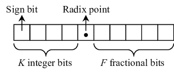
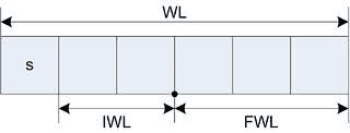
The simplest scheme one might come up with for a machine is a fixed point storage format. In fixed point notation, we write down all numbers with a certain number of digits before the decimal point and a certain number after the decimal point. With four digits (decimal) and two leading digits, we can, for example, write the number three as 0300 . This means $03.00$. Fixed point storage is the first variant I have sketched in our introductory thought experiment.

We immediately see that such a representation is not a fit for scientific computing. Let $x=3$ in the representation be divided by three. The result $x / 3=1.00$ suits our data structure. However, once we divide by three once more, we start to run into serious trouble. Indeed $1 / 3 \approx 0.33$ – which is the closest value to $1 / 3$ we can numerically encode – is already off the real result by $0.00 \overline{3}$.

You might be tempted to accept that you have a large error. But as a computational scientist, you neither can accept that most of your bits soon start to hold zeroes, i.e. no information at all, nor that your storage format is only suited to hold numbers from a very limited range (basically from $0.01$ to 30 and even here with quite some error).

Definition $4.1$ (Relative and absolute error) Computers always yield wrong results. To quantify this effect, we distinguish the absolute from the relative error. Let $x_M$ be the machine’s representation of $x$. The absolute round-off error then is given by
$$
e=\left|x_M-x\right| \text {. }
$$
The relative round-off error is given by
$$
\epsilon=\frac{e}{|x|}=\left|\frac{x_M-x}{x}\right|
$$
The reason behind inaccurate representations of numbers is that we work numerically. Each number in the computer is mapped onto a sequence of bits. This sequence is finite. So at one point, we have to cut the bits of the real number off. We introduce an error.

计算机代写|并行计算作业代写Parallel Computing代考|CSC267

并行计算代写

计算机代写|并行计算作业代写Parallel Computing代考|Numerical Versus Analytical Solutions

计算机是计算器。如果我们将某个问题传递给它们,例如“这里有两个物体通过重力相互作用”,它们会产生值作为解决方案:“物体最终位于位置X,和,和“。它们产生数值解。这与我们在学校做的很多数学不同。在那里,我们操纵公式并计算表达式,例如F(A,b)=∫Ab4XdX=2b2−2A2. 事实上,许多老师直到最后一分钟(或直到我们有了袖珍计算器)才让我们免于插入实际数字b和A.

在编程语言中,我们经常谈到变量。但是这些变量在程序运行的任何时候仍然包含数据。它们与数学公式中的变量根本不同,后者可能具有也可能不具有特定值。我们得出结论:有两种不同的方法来处理方程式:我们可以尝试为任意输入求解它们,即找到像这样的表达式F(A,b)=2b2−2A2. 一旦我们有了这样的解决方案,我们就可以插入不同的A和b值。该溶液是解析溶液。4在计算机上,我们通常以数字方式工作。我们提交数字,我们得到这些特定数字的答案。但是我们没有得到任何通用的解决方案。

定义3.2(解析解与数值解)如果我们通过公式重写(例如积分规则)求解方程,我们将获得变量的解析解。分析解决方案描述了一般系统行为。如果我们从一开始就针对一组特定的初始值对其进行求解,我们就会努力寻求数值解。

计算机产生数值解。这个说法不100%正确的。有产生符号解的计算机程序。它们被称为计算机代数系统。虽然它们非常强大,但它们无法始终找到解析解,并且如果没有解析解,显然不会产生结果。在本课程中,我们沿着数字路线走下去。

类似于数值解和解析解的这种区别,我们也可以区分我们如何操作公式。如果要确定导数∂吨和(吨)的和(吨)=吨2, 你知道∂吨和(吨)=2吨从学校。您可以象征性地操纵公式。在计算机中,您还可以评估∂吨和(吨)仅针对给定的输入。这通常包括一些算法近似值。在这种情况下,您再次以数字方式处理表达式。

计算机代写|并行计算作业代写Parallel Computing代考|Fixed Point Formats

人们可能想出的最简单的机器方案是定点存储格式。在定点表示法中,我们记下小数点前一定 位数和小数点后一定位数的所有数字。使用四位数字 (十进制) 和两位前导数字,例如,我们 可以将数字三写为 0300 。这意味着 $03.00$. 定点存储是我在介绍性思想实验中勾勒出的第一个 变体。
我们立即看到这种表示不适合科学计算。让 $x=3$ 在表示中被除以三。结果 $x / 3=1.00$ 适合 我们的数据结构。然而,一旦我们再次除以三,我们就开始遇到严重的麻烦。的确 $1 / 3 \approx 0.33$ – 这是最接近的值 $1 / 3$ 我们可以进行数字编码――已经脱离了真实结果 $0.00 \overline{3}$.
您可能会忍不住承认自己犯了一个大错误。但是作为一名计算科学家,您既不能接受您的大部 分位很快就会开始保存零,即根本没有信息,也不能接受您的存储格式仅适用于保存非常有限 范围内的数字(基本上从 $0.01$ 到 30 ,甚至这里有相当多的错误)。
定义4.1 (相对和绝对误差) 计算机总是产生错误的结果。为了量化这种影响,我们将绝对误 差与相对误差区分开来。让 $x_M$ 是机器的代表 $x$. 绝对舍入误差由下式给出
$$
e=\left|x_M-x\right| .
$$
相对舍入误差由下式给出
$$
\epsilon=\frac{e}{|x|}=\left|\frac{x_M-x}{x}\right|
$$
数字表示不准确背后的原因是我们以数字方式工作。计算机中的每个数字都映射到一个位序列 上。这个序列是有限的。所以在某一时刻,我们必须削减实数的位。我们引入了一个错误。

计算机代写|并行计算作业代写Parallel Computing代考 请认准statistics-lab™

统计代写请认准statistics-lab™. statistics-lab™为您的留学生涯保驾护航。

金融工程代写

金融工程是使用数学技术来解决金融问题。金融工程使用计算机科学、统计学、经济学和应用数学领域的工具和知识来解决当前的金融问题,以及设计新的和创新的金融产品。

非参数统计代写

非参数统计指的是一种统计方法,其中不假设数据来自于由少数参数决定的规定模型;这种模型的例子包括正态分布模型和线性回归模型。

广义线性模型代考

广义线性模型(GLM)归属统计学领域,是一种应用灵活的线性回归模型。该模型允许因变量的偏差分布有除了正态分布之外的其它分布。

术语 广义线性模型(GLM)通常是指给定连续和/或分类预测因素的连续响应变量的常规线性回归模型。它包括多元线性回归,以及方差分析和方差分析(仅含固定效应)。

有限元方法代写

有限元方法(FEM)是一种流行的方法,用于数值解决工程和数学建模中出现的微分方程。典型的问题领域包括结构分析、传热、流体流动、质量运输和电磁势等传统领域。

有限元是一种通用的数值方法,用于解决两个或三个空间变量的偏微分方程(即一些边界值问题)。为了解决一个问题,有限元将一个大系统细分为更小、更简单的部分,称为有限元。这是通过在空间维度上的特定空间离散化来实现的,它是通过构建对象的网格来实现的:用于求解的数值域,它有有限数量的点。边界值问题的有限元方法表述最终导致一个代数方程组。该方法在域上对未知函数进行逼近。[1] 然后将模拟这些有限元的简单方程组合成一个更大的方程系统,以模拟整个问题。然后,有限元通过变化微积分使相关的误差函数最小化来逼近一个解决方案。

tatistics-lab作为专业的留学生服务机构,多年来已为美国、英国、加拿大、澳洲等留学热门地的学生提供专业的学术服务,包括但不限于Essay代写,Assignment代写,Dissertation代写,Report代写,小组作业代写,Proposal代写,Paper代写,Presentation代写,计算机作业代写,论文修改和润色,网课代做,exam代考等等。写作范围涵盖高中,本科,研究生等海外留学全阶段,辐射金融,经济学,会计学,审计学,管理学等全球99%专业科目。写作团队既有专业英语母语作者,也有海外名校硕博留学生,每位写作老师都拥有过硬的语言能力,专业的学科背景和学术写作经验。我们承诺100%原创,100%专业,100%准时,100%满意。

随机分析代写


随机微积分是数学的一个分支,对随机过程进行操作。它允许为随机过程的积分定义一个关于随机过程的一致的积分理论。这个领域是由日本数学家伊藤清在第二次世界大战期间创建并开始的。

时间序列分析代写

随机过程,是依赖于参数的一组随机变量的全体,参数通常是时间。 随机变量是随机现象的数量表现,其时间序列是一组按照时间发生先后顺序进行排列的数据点序列。通常一组时间序列的时间间隔为一恒定值(如1秒,5分钟,12小时,7天,1年),因此时间序列可以作为离散时间数据进行分析处理。研究时间序列数据的意义在于现实中,往往需要研究某个事物其随时间发展变化的规律。这就需要通过研究该事物过去发展的历史记录,以得到其自身发展的规律。

回归分析代写

多元回归分析渐进(Multiple Regression Analysis Asymptotics)属于计量经济学领域,主要是一种数学上的统计分析方法,可以分析复杂情况下各影响因素的数学关系,在自然科学、社会和经济学等多个领域内应用广泛。

MATLAB代写

MATLAB 是一种用于技术计算的高性能语言。它将计算、可视化和编程集成在一个易于使用的环境中,其中问题和解决方案以熟悉的数学符号表示。典型用途包括:数学和计算算法开发建模、仿真和原型制作数据分析、探索和可视化科学和工程图形应用程序开发,包括图形用户界面构建MATLAB 是一个交互式系统,其基本数据元素是一个不需要维度的数组。这使您可以解决许多技术计算问题,尤其是那些具有矩阵和向量公式的问题,而只需用 C 或 Fortran 等标量非交互式语言编写程序所需的时间的一小部分。MATLAB 名称代表矩阵实验室。MATLAB 最初的编写目的是提供对由 LINPACK 和 EISPACK 项目开发的矩阵软件的轻松访问,这两个项目共同代表了矩阵计算软件的最新技术。MATLAB 经过多年的发展,得到了许多用户的投入。在大学环境中,它是数学、工程和科学入门和高级课程的标准教学工具。在工业领域,MATLAB 是高效研究、开发和分析的首选工具。MATLAB 具有一系列称为工具箱的特定于应用程序的解决方案。对于大多数 MATLAB 用户来说非常重要,工具箱允许您学习应用专业技术。工具箱是 MATLAB 函数(M 文件)的综合集合,可扩展 MATLAB 环境以解决特定类别的问题。可用工具箱的领域包括信号处理、控制系统、神经网络、模糊逻辑、小波、仿真等。

R语言代写问卷设计与分析代写
PYTHON代写回归分析与线性模型代写
MATLAB代写方差分析与试验设计代写
STATA代写机器学习/统计学习代写
SPSS代写计量经济学代写
EVIEWS代写时间序列分析代写
EXCEL代写深度学习代写
SQL代写各种数据建模与可视化代写

计算机代写|并行计算作业代写Parallel Computing代考|CSE415

如果你也在 怎样代写并行计算Parallel Computing这个学科遇到相关的难题,请随时右上角联系我们的24/7代写客服。

并行计算是指将较大的问题分解成较小的、独立的、通常是类似的部分,由通过共享内存通信的多个处理器同时执行的过程,其结果在完成后作为整体算法的一部分被合并。

statistics-lab™ 为您的留学生涯保驾护航 在代写并行计算Parallel Computing方面已经树立了自己的口碑, 保证靠谱, 高质且原创的统计Statistics代写服务。我们的专家在代写并行计算Parallel Computing代写方面经验极为丰富,各种代写并行计算Parallel Computing相关的作业也就用不着说。

我们提供的并行计算Parallel Computing及其相关学科的代写,服务范围广, 其中包括但不限于:

  • Statistical Inference 统计推断
  • Statistical Computing 统计计算
  • Advanced Probability Theory 高等楖率论
  • Advanced Mathematical Statistics 高等数理统计学
  • (Generalized) Linear Models 广义线性模型
  • Statistical Machine Learning 统计机器学习
  • Longitudinal Data Analysis 纵向数据分析
  • Foundations of Data Science 数据科学基础
计算机代写|并行计算作业代写Parallel Computing代考|CSE415

计算机代写|并行计算作业代写Parallel Computing代考|The N-Body Problem

Given are $N$ bodies (planets, e.g.) out there in space. They interact with each other through gravity. Let body 1 be described by its position $p_1=\left(p_{x, 1}, p_{y, 1}, p_{z, 1}\right)^T \in$ $\mathbb{R}^3$ (a vector) and its mass $m_1$. Furthermore, it has a certain velocity $v_1=$ $\left(v_{x, 1}, v_{y, 1}, v_{z, 1}\right)^T \in \mathbb{R}^3$ which is a vector again. Body 2 is defined analogously. Body 1 experiences a force
$$
F_1=G \frac{m_1 \cdot m_2}{\left|p_1-p_2\right|_2^2} \cdot \frac{\left(p_2-p_1\right)}{\left|p_1-p_2\right|_2} .
$$
If there are more than two objects, then Body 1 also gets a contribution from Body 3,4 , and so forth. The forces simply sum up. We furthermore know that
$$
\begin{aligned}
\partial_t v_1(t) & =\frac{F_1}{m_1} \text { and } \
\partial_t p_1(t) & =v_1(t) .
\end{aligned}
$$
This is a complete mathematical model of the reality. It highlights in (3.2) and (3.3) that velocity and position of our object depend on time. These equations are our whole theory of how the world out there in space behaves (cmp. Chap. 1) in a Newton sense. Einstein has later revised this model. ${ }^2$

The expressions $\partial_t y(t)=\frac{\partial}{\partial t} y(t)$ both denote the derivation of a function $y(t)$. Often, we drop the $(t)$ parameter-we have already done so for $F$ above. For the second derivative, there are various notations that all mean the same: $\partial_t \partial_t y=\partial_{t t} y=\frac{\partial \partial}{\partial t \partial t} y$. I often use $\partial_t^{(2)}$. This notation makes it easy to specify arbitrary high derivatives.

计算机代写|并行计算作业代写Parallel Computing代考|Time Discretisation: Running a Movie

Let’s assume that we live in a movie universe where the whole universe runs at 60 frames per second. In each frame, we know all objects $p_n$ as well as their velocities $v_n$. We can compute the forces at this very frame. They push the particles, i.e. they alter their velocities. Due to the (changed) velocity, all objects end up at a different place in the next frame (Fig. 3.1). The longer the time in-between two frames, the more the particles can change their position (the velocity acts longer). To make the impact of our force pushes realistic, the forces are the bigger the bigger the time in-between two frames, too. The more frames per second we use, the more accurate our universe. With the time step size going to zero, we eventually end up with the real thing.

The construction of the movie universe from the real one is called discretisation. We know that time is continuous-at least at our scale-and computers struggle to hold things that are infinitely small and detailed. After all, we have finite memory, finite compute power and finite compute time. So we sample or discretise the time and track the solution in time steps. Let dt be the time step size, i.e. the time in-between two snapshots. ${ }^3$ Our computer program simulation the space bodies then reads as follows.

This code is not particular sophisticated. For example, we do not exploit any symmetries between the particles. It is also not necessary to introduce force variables in this code, as we could directly add the force contributions to the object velocities. I leave it to the reader to come up with more intelligent versions of this code. For the time being, it is sufficient to us to know that the scheme we have just implemented is an explicit Euler.

Writing data into a file is very slow. Therefore, programs typically give you the opportunity to specify the time in-between two snapshots. This time is usually way bigger than dt. Don’t mix them up: You step through your simulation with dt and then every $k$ of these time steps you write a snapshot. As alternative to time steps, you can specify a second DT after which you write the snapshot.

计算机代写|并行计算作业代写Parallel Computing代考|CSE415

并行计算代写

计算机代写|并行计算作业代写Parallel Computing代考|The N-Body Problem

给出的是 $N$ 太空中的物体 (例如行星) 。它们通过引力相互作用。让 body 1 用它的位置来描 述 $p_1=\left(p_{x, 1}, p_{y, 1}, p_{z, 1}\right)^T \in \mathbb{R}^3$ (矢量) 及其质量 $m_1$. 此外,它具有一定的速度 $v_1=$ $\left(v_{x, 1}, v_{y, 1}, v_{z, 1}\right)^T \in \mathbb{R}^3$ 这又是一个向量。主体 2 的定义类似。身体 1 受到力
$$
F_1=G \frac{m_1 \cdot m_2}{\left|p_1-p_2\right|2^2} \cdot \frac{\left(p_2-p_1\right)}{\left|p_1-p_2\right|_2} . $$ 如果有两个以上的对象,那么 Body 1 也会从 Body 3,4 获得贡献,依此类推。力量简单总结。 我们还知道 $$ \partial_t v_1(t)=\frac{F_1}{m_1} \text { and } \partial_t p_1(t)=v_1(t) . $$ 这是一个完整的现实数学模型。它在 (3.2) 和 (3.3) 中强调我们对象的速度和位置取决于时间。 这些方程式是我们在牛顿意义上关于太空中的世界如何运行的整个理论 (cmp。第1章)。爱 因斯坦后来修改了这个模型。 ${ }^2$ 表达式 $\partial_t y(t)=\frac{\partial}{\partial t} y(t)$ 都表示函数的推导 $y(t)$. 通常,我们丟弃 $(t)$ 参数-我们已经这样做了 $F$ 多于。对于二阶导数,有多种表示法都是相同的: $\partial_t \partial_t y=\partial{t t} y=\frac{\partial \partial}{\partial t \partial t} y$. 我经常用 $\partial_t^{(2)}$. 这种表示法使得指定任意高阶导数变得容易。

计算机代写|并行计算作业代写Parallel Computing代考|Time Discretisation: Running a Movie

假设我们生活在一个电影宇宙中,整个宇宙以每秒 60 帧的速度运行。在每一帧中,我们知道所有对象pn以及它们的速度在n. 我们可以在这个坐标系中计算力。它们推动粒子,即它们改变它们的速度。由于(改变的)速度,所有对象在下一帧中最终都位于不同的位置(图 3.1)。两帧之间的时间越长,粒子改变位置的可能性就越大(速度作用的时间越长)。为了使我们的力推的影响真实,力越大,两帧之间的时间也越长。我们每秒使用的帧数越多,我们的宇宙就越准确。随着时间步长变为零,我们最终得到了真实的东西。

从真实世界构建电影世界称为离散化。我们知道时间是连续的——至少在我们的尺度上是这样——而计算机很难容纳无限小和详细的东西。毕竟,我们拥有有限的内存、有限的计算能力和有限的计算时间。因此,我们对时间进行采样或离散化,并按时间步长跟踪解决方案。令 dt 为时间步长,即两个快照之间的时间。3我们的计算机程序模拟空间体然后读取如下。

这段代码不是特别复杂。例如,我们不利用粒子之间的任何对称性。也没有必要在此代码中引入力变量,因为我们可以直接将力贡献添加到对象速度中。我留给读者想出此代码的更智能版本。目前,我们只要知道我们刚刚实现的方案是显式欧拉方案就足够了。

将数据写入文件非常慢。因此,程序通常会让您有机会指定两个快照之间的时间。这个时间通常比 dt 大得多。不要混淆它们:您使用 dt 逐步完成模拟,然后每k这些时间步你写一个快照。作为时间步长的替代方法,您可以指定第二个 DT,然后再写入快照。

计算机代写|并行计算作业代写Parallel Computing代考 请认准statistics-lab™

统计代写请认准statistics-lab™. statistics-lab™为您的留学生涯保驾护航。

金融工程代写

金融工程是使用数学技术来解决金融问题。金融工程使用计算机科学、统计学、经济学和应用数学领域的工具和知识来解决当前的金融问题,以及设计新的和创新的金融产品。

非参数统计代写

非参数统计指的是一种统计方法,其中不假设数据来自于由少数参数决定的规定模型;这种模型的例子包括正态分布模型和线性回归模型。

广义线性模型代考

广义线性模型(GLM)归属统计学领域,是一种应用灵活的线性回归模型。该模型允许因变量的偏差分布有除了正态分布之外的其它分布。

术语 广义线性模型(GLM)通常是指给定连续和/或分类预测因素的连续响应变量的常规线性回归模型。它包括多元线性回归,以及方差分析和方差分析(仅含固定效应)。

有限元方法代写

有限元方法(FEM)是一种流行的方法,用于数值解决工程和数学建模中出现的微分方程。典型的问题领域包括结构分析、传热、流体流动、质量运输和电磁势等传统领域。

有限元是一种通用的数值方法,用于解决两个或三个空间变量的偏微分方程(即一些边界值问题)。为了解决一个问题,有限元将一个大系统细分为更小、更简单的部分,称为有限元。这是通过在空间维度上的特定空间离散化来实现的,它是通过构建对象的网格来实现的:用于求解的数值域,它有有限数量的点。边界值问题的有限元方法表述最终导致一个代数方程组。该方法在域上对未知函数进行逼近。[1] 然后将模拟这些有限元的简单方程组合成一个更大的方程系统,以模拟整个问题。然后,有限元通过变化微积分使相关的误差函数最小化来逼近一个解决方案。

tatistics-lab作为专业的留学生服务机构,多年来已为美国、英国、加拿大、澳洲等留学热门地的学生提供专业的学术服务,包括但不限于Essay代写,Assignment代写,Dissertation代写,Report代写,小组作业代写,Proposal代写,Paper代写,Presentation代写,计算机作业代写,论文修改和润色,网课代做,exam代考等等。写作范围涵盖高中,本科,研究生等海外留学全阶段,辐射金融,经济学,会计学,审计学,管理学等全球99%专业科目。写作团队既有专业英语母语作者,也有海外名校硕博留学生,每位写作老师都拥有过硬的语言能力,专业的学科背景和学术写作经验。我们承诺100%原创,100%专业,100%准时,100%满意。

随机分析代写


随机微积分是数学的一个分支,对随机过程进行操作。它允许为随机过程的积分定义一个关于随机过程的一致的积分理论。这个领域是由日本数学家伊藤清在第二次世界大战期间创建并开始的。

时间序列分析代写

随机过程,是依赖于参数的一组随机变量的全体,参数通常是时间。 随机变量是随机现象的数量表现,其时间序列是一组按照时间发生先后顺序进行排列的数据点序列。通常一组时间序列的时间间隔为一恒定值(如1秒,5分钟,12小时,7天,1年),因此时间序列可以作为离散时间数据进行分析处理。研究时间序列数据的意义在于现实中,往往需要研究某个事物其随时间发展变化的规律。这就需要通过研究该事物过去发展的历史记录,以得到其自身发展的规律。

回归分析代写

多元回归分析渐进(Multiple Regression Analysis Asymptotics)属于计量经济学领域,主要是一种数学上的统计分析方法,可以分析复杂情况下各影响因素的数学关系,在自然科学、社会和经济学等多个领域内应用广泛。

MATLAB代写

MATLAB 是一种用于技术计算的高性能语言。它将计算、可视化和编程集成在一个易于使用的环境中,其中问题和解决方案以熟悉的数学符号表示。典型用途包括:数学和计算算法开发建模、仿真和原型制作数据分析、探索和可视化科学和工程图形应用程序开发,包括图形用户界面构建MATLAB 是一个交互式系统,其基本数据元素是一个不需要维度的数组。这使您可以解决许多技术计算问题,尤其是那些具有矩阵和向量公式的问题,而只需用 C 或 Fortran 等标量非交互式语言编写程序所需的时间的一小部分。MATLAB 名称代表矩阵实验室。MATLAB 最初的编写目的是提供对由 LINPACK 和 EISPACK 项目开发的矩阵软件的轻松访问,这两个项目共同代表了矩阵计算软件的最新技术。MATLAB 经过多年的发展,得到了许多用户的投入。在大学环境中,它是数学、工程和科学入门和高级课程的标准教学工具。在工业领域,MATLAB 是高效研究、开发和分析的首选工具。MATLAB 具有一系列称为工具箱的特定于应用程序的解决方案。对于大多数 MATLAB 用户来说非常重要,工具箱允许您学习应用专业技术。工具箱是 MATLAB 函数(M 文件)的综合集合,可扩展 MATLAB 环境以解决特定类别的问题。可用工具箱的领域包括信号处理、控制系统、神经网络、模糊逻辑、小波、仿真等。

R语言代写问卷设计与分析代写
PYTHON代写回归分析与线性模型代写
MATLAB代写方差分析与试验设计代写
STATA代写机器学习/统计学习代写
SPSS代写计量经济学代写
EVIEWS代写时间序列分析代写
EXCEL代写深度学习代写
SQL代写各种数据建模与可视化代写

计算机代写|并行计算作业代写Parallel Computing代考|CS149

如果你也在 怎样代写并行计算Parallel Computing这个学科遇到相关的难题,请随时右上角联系我们的24/7代写客服。

并行计算是指将较大的问题分解成较小的、独立的、通常是类似的部分,由通过共享内存通信的多个处理器同时执行的过程,其结果在完成后作为整体算法的一部分被合并。

statistics-lab™ 为您的留学生涯保驾护航 在代写并行计算Parallel Computing方面已经树立了自己的口碑, 保证靠谱, 高质且原创的统计Statistics代写服务。我们的专家在代写并行计算Parallel Computing代写方面经验极为丰富,各种代写并行计算Parallel Computing相关的作业也就用不着说。

我们提供的并行计算Parallel Computing及其相关学科的代写,服务范围广, 其中包括但不限于:

  • Statistical Inference 统计推断
  • Statistical Computing 统计计算
  • Advanced Probability Theory 高等楖率论
  • Advanced Mathematical Statistics 高等数理统计学
  • (Generalized) Linear Models 广义线性模型
  • Statistical Machine Learning 统计机器学习
  • Longitudinal Data Analysis 纵向数据分析
  • Foundations of Data Science 数据科学基础
计算机代写|并行计算作业代写Parallel Computing代考|CS149

计算机代写|并行计算作业代写Parallel Computing代考|Dennard Scaling

Definition $2.1$ (Dennard scaling) The power cost $P$ to drive a transistor follows roughly
$$
P=\alpha \cdot C F V^2 .
$$
This law is called Dennard scaling.
$C$ is the capacitance, i.e. encodes the size of the individual transistors. I use $C$ here for historic reasons. In the remainder of this manuscript, $C$ is some generic constant without a particular meaning. $F$ is the frequency and $V$ the voltage. $\alpha$ is some fixed constant so we can safely skip it in our follow-up discussions. Note that the original Dennard scaling ignores that we also have some leakage. Leakage did not play a major role when the law was formulated in 1974.

Dennard’s scaling law is all about power. For both chip designers and computing centres buying and running chips, controlling the power envelope of a chip is a sine qua non, as

  • buying power is expensive, and as
  • a chip “converts” power into heat. To get the heat out of the system again requires even more power to drive fans, pumps and cooling liquids. But if we don’t get it out of the system on time, the chip will eventually melt down.

While we want to bring the power needs down, we still want a computer to be as capable as possible. That means, it should be able to do as many calculations per seconds as possible. The Dennard scaling tells us that we have only three degrees of freedom:

  1. Reduce the voltage. This is clearly the gold solution as the $V$ term enters the equation squared. Reducing the voltage however is not trivial: If we reduce it too much, the transistors don’t switch reliably anymore. As long as we need a reliable chip, i.e. a chip that always gives us the right answer, we work already close to the minimum voltage limit with modern architectures.
  2. Reduce the transistor size. Chip vendors always try to decrease transistor sizes with the launch of most new chip factories or assembly lines. Unfortunately, this option now is, more or less, maxed out. You can’t go below a few atoms. A further shrinkage of transistors means that the reliability of the machine starts to suffer-we ultimately might have to add additional transistors to handle the errors which once more need energy. Most importantly, smaller chips are more expensive to build (if they have to meet high quality constraints) which makes further shrinking less attractive.
  3. Reduce the frequency. If we reduce the frequency, we usually also get away with a slightly lower voltage, so this amplifies the savings effect further. However, we want to have a faster transistor, not a slower one!

计算机代写|并行计算作业代写Parallel Computing代考|The Three Layers of Parallelism

With Moore’s law continuing to hold and a break-down of Dennard scaling (frequency cannot be increased anymore at a given power envelope per transistor), there is a “new” kid on the block that helps us to build more powerful computers. This one eventually allows Computational $\mathrm{X}$ to run more challenging simulations. Actually, there are three new kids around that dominate code development today (Fig. 2.2). However, they all are flavours of one common pattern:

  1. The parallelism in the computer increases, as modern computers still can do one addition or multiplication or …on one or two pieces of data in one (abstract) step. ${ }^2$ They apply with the same operation to a whole vector of entries in one rush. We call this vector parallelism.
  2. The parallelism in the computer increases, as modern CPUs do not only host one core but an ensemble of cores per chip. Since this multicore idea implies that all cores share their memory we call this shared memory parallelism.
  3. The parallelism in the computer increases, as modern modern supercomputers consist of thousands of compute nodes. A compute nodes is our term for a classic computer which “speaks” to other computers via a network. Since the individual nodes are independent computers, they do not share their memory. Each one has memory of its own. We therefore call this distributed memory parallelism.

The three levels of parallelism have different potential to speed up calculations. This potential depends on the character of the underlying calculations as well as on the hardware, while the boundaries in-between the parallelism flavours are often blurred.
We discuss ways to program two out of three levels of parallelism here, but skip the distributed memory world that unfolds its full power in multi-node supercomputers. The role of accelerators (GPGPUs) in such a classification spans all three rubrics: An accelerator is a computer within the computer including its own memory. GPGPUs themselves rely heavily on both vectorisation and multicore processing: They host multiple (streaming) processors, and the individual processors can handle one instruction acting on multiple pieces of data per step.

计算机代写|并行计算作业代写Parallel Computing代考|CS149

并行计算代写

计算机代写|并行计算作业代写Parallel Computing代考|Dennard Scaling

定义2.1(登纳德缩放)功率成本P驱动晶体管大致如下

P=A⋅CF在2.
该定律称为登纳德缩放。
C是电容,即对单个晶体管的大小进行编码。我用C这里是因为历史原因。在这份手稿的其余部分,C是一些没有特定含义的通用常量。F是频率和在电压。A是一些固定常数,因此我们可以在后续讨论中安全地跳过它。请注意,原始的 Dennard 缩放忽略了我们也有一些泄漏。1974 年制定法律时,泄漏并未发挥主要作用。

丹纳德的比例定律是关于权力的。对于购买和运行芯片的芯片设计师和计算中心来说,控制芯片的功率包络是一个必要条件,因为

  • 购买力是昂贵的,并且作为
  • 芯片将电能“转换”为热能。要再次将热量从系统中排出,需要更多的动力来驱动风扇、泵和冷却液。但如果我们不及时将其从系统中取出,芯片最终会熔化。

虽然我们想要降低电力需求,但我们仍然希望计算机尽可能地强大。这意味着,它应该能够每秒进行尽可能多的计算。Dennard 标度告诉我们,我们只有三个自由度:

  1. 降低电压。这显然是黄金解决方案在项进入方程的平方。然而,降低电压并非微不足道:如果我们将电压降低太多,晶体管将不再可靠地切换。只要我们需要一个可靠的芯片,即始终为我们提供正确答案的芯片,我们就已经接近现代架构的最低电压限制。
  2. 减小晶体管尺寸。芯片供应商总是试图通过推出大多数新芯片工厂或装配线来减小晶体管尺寸。不幸的是,这个选项现在或多或少已经用完了。你不能低于几个原子。晶体管的进一步缩小意味着机器的可靠性开始受到影响——我们最终可能不得不添加额外的晶体管来处理再次需要能量的错误。最重要的是,较小的芯片制造成本更高(如果它们必须满足高质量限制),这使得进一步缩小的吸引力降低。
  3. 降低频率。如果我们降低频率,我们通常也会以略低的电压逃脱,因此这进一步放大了节省效果。然而,我们想要一个更快的晶体管,而不是更慢的!

计算机代写|并行计算作业代写Parallel Computing代考|The Three Layers of Parallelism

随着摩尔定律的继续适用和登纳德定标法的失效(在每个晶体管的给定功率包络下,频率不能再增加),块上出现了一个“新”孩子,可以帮助我们构建更强大的计算机。这个最终允许计算X运行更具挑战性的模拟。实际上,当今有三个新手主导着代码开发(图 2.2)。然而,它们都是一种常见模式的变体:

  1. 计算机中的并行性增加了,因为现代计算机仍然可以在一个(抽象的)步骤中对一个或两个数据进行加法或乘法或……。2他们将相同的操作一次性应用于整个条目向量。我们称之为向量并行性。
  2. 计算机中的并行性增加了,因为现代 CPU 不仅承载一个内核,而且每个芯片承载一组内核。由于这种多核思想意味着所有内核共享它们的内存,我们称之为共享内存并行。
  3. 随着现代现代超级计算机由数千个计算节点组成,计算机中的并行性增加了。计算节点是我们对经典计算机的术语,它通过网络与其他计算机“对话”。由于各个节点是独立的计算机,因此它们不共享内存。每个人都有自己的记忆。因此,我们将此称为分布式内存并行性。

三个级别的并行性具有不同的加速计算的潜力。这种潜力取决于底层计算的特性以及硬件,而并行风格之间的界限通常是模糊的。
我们在这里讨论了对三个并行级别中的两个进行编程的方法,但跳过了在多节点超级计算机中展现其全部功能的分布式内存世界。加速器 (GPGPU) 在此类分类中的作用涵盖所有三个标准:加速器是计算机中的计算机,包括其自身的内存。GPGPU 本身在很大程度上依赖于矢量化和多核处理:它们托管多个(流)处理器,并且各个处理器可以处理一条指令,该指令每一步作用于多条数据。

计算机代写|并行计算作业代写Parallel Computing代考 请认准statistics-lab™

统计代写请认准statistics-lab™. statistics-lab™为您的留学生涯保驾护航。

金融工程代写

金融工程是使用数学技术来解决金融问题。金融工程使用计算机科学、统计学、经济学和应用数学领域的工具和知识来解决当前的金融问题,以及设计新的和创新的金融产品。

非参数统计代写

非参数统计指的是一种统计方法,其中不假设数据来自于由少数参数决定的规定模型;这种模型的例子包括正态分布模型和线性回归模型。

广义线性模型代考

广义线性模型(GLM)归属统计学领域,是一种应用灵活的线性回归模型。该模型允许因变量的偏差分布有除了正态分布之外的其它分布。

术语 广义线性模型(GLM)通常是指给定连续和/或分类预测因素的连续响应变量的常规线性回归模型。它包括多元线性回归,以及方差分析和方差分析(仅含固定效应)。

有限元方法代写

有限元方法(FEM)是一种流行的方法,用于数值解决工程和数学建模中出现的微分方程。典型的问题领域包括结构分析、传热、流体流动、质量运输和电磁势等传统领域。

有限元是一种通用的数值方法,用于解决两个或三个空间变量的偏微分方程(即一些边界值问题)。为了解决一个问题,有限元将一个大系统细分为更小、更简单的部分,称为有限元。这是通过在空间维度上的特定空间离散化来实现的,它是通过构建对象的网格来实现的:用于求解的数值域,它有有限数量的点。边界值问题的有限元方法表述最终导致一个代数方程组。该方法在域上对未知函数进行逼近。[1] 然后将模拟这些有限元的简单方程组合成一个更大的方程系统,以模拟整个问题。然后,有限元通过变化微积分使相关的误差函数最小化来逼近一个解决方案。

tatistics-lab作为专业的留学生服务机构,多年来已为美国、英国、加拿大、澳洲等留学热门地的学生提供专业的学术服务,包括但不限于Essay代写,Assignment代写,Dissertation代写,Report代写,小组作业代写,Proposal代写,Paper代写,Presentation代写,计算机作业代写,论文修改和润色,网课代做,exam代考等等。写作范围涵盖高中,本科,研究生等海外留学全阶段,辐射金融,经济学,会计学,审计学,管理学等全球99%专业科目。写作团队既有专业英语母语作者,也有海外名校硕博留学生,每位写作老师都拥有过硬的语言能力,专业的学科背景和学术写作经验。我们承诺100%原创,100%专业,100%准时,100%满意。

随机分析代写


随机微积分是数学的一个分支,对随机过程进行操作。它允许为随机过程的积分定义一个关于随机过程的一致的积分理论。这个领域是由日本数学家伊藤清在第二次世界大战期间创建并开始的。

时间序列分析代写

随机过程,是依赖于参数的一组随机变量的全体,参数通常是时间。 随机变量是随机现象的数量表现,其时间序列是一组按照时间发生先后顺序进行排列的数据点序列。通常一组时间序列的时间间隔为一恒定值(如1秒,5分钟,12小时,7天,1年),因此时间序列可以作为离散时间数据进行分析处理。研究时间序列数据的意义在于现实中,往往需要研究某个事物其随时间发展变化的规律。这就需要通过研究该事物过去发展的历史记录,以得到其自身发展的规律。

回归分析代写

多元回归分析渐进(Multiple Regression Analysis Asymptotics)属于计量经济学领域,主要是一种数学上的统计分析方法,可以分析复杂情况下各影响因素的数学关系,在自然科学、社会和经济学等多个领域内应用广泛。

MATLAB代写

MATLAB 是一种用于技术计算的高性能语言。它将计算、可视化和编程集成在一个易于使用的环境中,其中问题和解决方案以熟悉的数学符号表示。典型用途包括:数学和计算算法开发建模、仿真和原型制作数据分析、探索和可视化科学和工程图形应用程序开发,包括图形用户界面构建MATLAB 是一个交互式系统,其基本数据元素是一个不需要维度的数组。这使您可以解决许多技术计算问题,尤其是那些具有矩阵和向量公式的问题,而只需用 C 或 Fortran 等标量非交互式语言编写程序所需的时间的一小部分。MATLAB 名称代表矩阵实验室。MATLAB 最初的编写目的是提供对由 LINPACK 和 EISPACK 项目开发的矩阵软件的轻松访问,这两个项目共同代表了矩阵计算软件的最新技术。MATLAB 经过多年的发展,得到了许多用户的投入。在大学环境中,它是数学、工程和科学入门和高级课程的标准教学工具。在工业领域,MATLAB 是高效研究、开发和分析的首选工具。MATLAB 具有一系列称为工具箱的特定于应用程序的解决方案。对于大多数 MATLAB 用户来说非常重要,工具箱允许您学习应用专业技术。工具箱是 MATLAB 函数(M 文件)的综合集合,可扩展 MATLAB 环境以解决特定类别的问题。可用工具箱的领域包括信号处理、控制系统、神经网络、模糊逻辑、小波、仿真等。

R语言代写问卷设计与分析代写
PYTHON代写回归分析与线性模型代写
MATLAB代写方差分析与试验设计代写
STATA代写机器学习/统计学习代写
SPSS代写计量经济学代写
EVIEWS代写时间序列分析代写
EXCEL代写深度学习代写
SQL代写各种数据建模与可视化代写

计算机代写|并行计算作业代写Parallel Computing代考|Temporary Variables

如果你也在 怎样代写并行计算Parallel Computing这个学科遇到相关的难题,请随时右上角联系我们的24/7代写客服。

并行计算是指将较大的问题分解成较小的、独立的、通常是类似的部分,由通过共享内存通信的多个处理器同时执行的过程,其结果在完成后作为整体算法的一部分被合并。

statistics-lab™ 为您的留学生涯保驾护航 在代写并行计算Parallel Computing方面已经树立了自己的口碑, 保证靠谱, 高质且原创的统计Statistics代写服务。我们的专家在代写并行计算Parallel Computing代写方面经验极为丰富,各种代写并行计算Parallel Computing相关的作业也就用不着说。

我们提供的并行计算Parallel Computing及其相关学科的代写,服务范围广, 其中包括但不限于:

  • Statistical Inference 统计推断
  • Statistical Computing 统计计算
  • Advanced Probability Theory 高等楖率论
  • Advanced Mathematical Statistics 高等数理统计学
  • (Generalized) Linear Models 广义线性模型
  • Statistical Machine Learning 统计机器学习
  • Longitudinal Data Analysis 纵向数据分析
  • Foundations of Data Science 数据科学基础
计算机代写|并行计算作业代写Parallel Computing代考|Temporary Variables

计算机代写|并行计算作业代写Parallel Computing代考|Temporary Variables

A temporary variable is any variable that is the target of a direct, nonindexed assignment, but is not a reduction variable. In the following parfor-loop, a and $d$ are temporary variables:
$\mathrm{a}=\theta$;
$z=\theta$;
$r=\operatorname{rand}(1,10)$;
parfor $i=1: 10$
a $=i ; \quad$ \& Variable a is temporary
$z=z+i ;$
$z=z+i$ if $i<=5$ end end
end
In contrast to the behavior of a for-loop, MATLAB clears any temporary variables before each
iteration of a parfor-loop. To help ensure the independence of iterations, the values of temporary
variables cannot be passed from one iteration of the loop to another. Therefore, temporary variables
must be set inside the body of a parfor-loop, so that their values are defined separately for each
iteration.
MATLAB does not send temporary variables back to the client. A temporary variable in a parfor-loop has no effect on a variable with the same name that exists outside the loop. This behavior is different from ordinary for-loops.

计算机代写|并行计算作业代写Parallel Computing代考|Uninitialized Temporaries

Temporary variables in a parfor-loop are cleared at the beginning of every iteration. MATLAB can sometimes detect cases in which loop iterations use a temporary variable before it is set in that iteration. In this case, MATLAB issues a static error rather than a run-time error. There is little point in allowing execution to proceed if a run-time error is guaranteed to occur. This kind of error often arises because of confusion between for and parfor, especially regarding the rules of classification of variables. For example:
b = true;
parfor $i=1: n$
if b Eas some_condition(i)
do_something(i);
$b=$ false;
end
$b=$ true;
parfor $i=1: n$
if b Eas some_condition(i)
do_something(i);
$\quad b=$ false;
end
end
This loop is acceptable as an ordinary for-loop. However, as a parfor-loop, b is a temporary variable because it occurs directly as the target of an assignment inside the loop. Therefore it is cleared at the start of each iteration, so its use in the condition of the if is guaranteed to be uninitialized. If you change parfor to for, the value of $b$ assumes sequential execution of the loop. In that case, do_something $(i)$ is executed only for the lower values of $i$ until b is set false.

计算机代写|并行计算作业代写Parallel Computing代考|Temporary Variables Intended as Reduction Variables

Another common cause of uninitialized temporaries can arise when you have a variable that you intended to be a reduction variable. However, if you use it elsewhere in the loop, then it is classified as a temporary variable. For example:
$s=\theta$;
parfor $i=1: n$
$s=s+f(i)$;
if (s> whatever)
end
end
Another common cause of uninitialized temporaries can arise when you have a variable that you
intended to be a reduction variable. However, if you use it elsewhere in the loop, then it is classified
as a temporary variable. For example:
$s=0$;
parfor $i=1: n$
$\quad s=s+f(i)$;
$\quad$ if $(s>$ whatever)
end
end
If the only occurrences of s are the two in the first statement of the body, s would be classified as a
reduction variable. But in this example, $s$ is not a reduction variable because it has a use outside of
reduction assignments in the line s $>$ whatever. Because s is the target of an assignment (in the
first statement), it is a temporary. Therefore MATLAB issues an error, but points out the possible
connection with reduction.
If you change parfor to for, the use of s outside the reduction assignment relies on the iterations
being performed in a particular order. In a parfor-loop, it matters that the loop “does not care”
about the value of a reduction variable as it goes along. It is only after the loop that the reduction
value becomes usable.
If the only occurrences of s are the two in the first statement of the body, s would be classified as a
reduction variable. But in this example, $s$ is not a reduction variable because it has a use outside of
reduction assignments in the line $s>$ whatever. Because $s$ is the target of an assignment (in the
first statement), it is a temporary. Therefore MATLAB issues an error, but points out the possible
connection with reduction.
If you change parfor to for, the use of s outside the reduction assignment relies on the iterations being performed in a particular order. In a parfor-loop, it matters that the loop “does not care” about the value of a reduction variable as it goes along. It is only after the loop that the reduction value becomes usable.

计算机代写|并行计算作业代写Parallel Computing代考|Temporary Variables

并行计算代写

计算机代写|并行计算作业代写Parallel Computing代考|Temporary Variables

临时变量是作为直接、非索引赋值的目标的任何变量,但不是归约变量。在下面的 parfor 循环中,a 和d是临时变量:
一种=θ;
和=θ;
r=兰特⁡(1,10);
帕尔福一世=1:10
一种=一世;\& 变量 a 是临时的
和=和+一世;
和=和+一世如果一世<=5end end
end
与 for 循环的行为相反,MATLAB 在
parfor 循环的每次迭代之前清除所有临时变量。为了帮助确保迭代的独立性,临时
变量的值不能从循环的一个迭代传递到另一个迭代。
因此,必须在 parfor 循环的主体内设置临时变量,以便为每次
迭代单独定义它们的值。
MATLAB 不会将临时变量发送回客户端。parfor 循环中的临时变量对循环外存在的同名变量没有影响。这种行为不同于普通的 for 循环。

计算机代写|并行计算作业代写Parallel Computing代考|Uninitialized Temporaries

parfor 循环中的临时变量在每次迭代开始时都会被清除。MATLAB 有时可以检测到循环迭代在该迭代中设置之前使用临时变量的情况。在这种情况下,MATLAB 会发出静态错误而不是运行时错误。如果保证会发生运行时错误,则允许继续执行几乎没有意义。这种错误通常是由于混淆了 for 和 parfor 造成的,尤其是在变量分类规则方面。例如:
b = true;
帕尔福一世=1:n
if b Eas some_condition(i)
do_something(i);
b=错误的;

b=真的;
帕尔福一世=1:n
if b Eas some_condition(i)
do_something(i);
b=错误的;
end
end
这个循环可以作为一个普通的for循环来接受。但是,作为 parfor 循环,b 是一个临时变量,因为它直接作为循环内的赋值目标出现。因此它在每次迭代开始时被清除,因此它在 if 条件下的使用保证未初始化。如果将 parfor 更改为 for,则值为b假定循环的顺序执行。在这种情况下, do_something(一世)仅对较低的值执行一世直到 b 设置为假。

计算机代写|并行计算作业代写Parallel Computing代考|Temporary Variables Intended as Reduction Variables

当您有一个打算作为归约变量的变量时,可能会出现未初始化临时变量的另一个常见原因。但是,如果您在循环中的其他地方使用它,则它被归类为临时变量。例如:
s=θ;
帕尔福一世=1:n
s=s+F(一世);
if (s> whatever)
end
end
当你有一个变量,你
打算成为一个归约变量时,可能会出现另一个未初始化临时变量的常见原因。但是,如果您在循环中的其他地方使用它,则它被归类
为临时变量。例如:
s=0;
帕尔福一世=1:n
s=s+F(一世);
如果(s>不管)
end
end
如果 s 的唯一出现是主体的第一个语句中的两个,则 s 将被归类为
归约变量。但在这个例子中,s不是归约变量,因为它
在行 s 中的归约赋值之外有用途>任何。因为 s 是赋值的目标(在
第一条语句中),所以它是临时的。因此 MATLAB 发出错误,但指出可能
与归约有关。
如果将 parfor 更改为 for,则在归约赋值之外使用 s 依赖于
以特定顺序执行的迭代。在 parfor 循环中,重要的是循环“不关心”
减少变量的值。只有在循环之后,减少
值才可用。
如果 s 的唯一出现是主体的第一个语句中的两个,则 s 将被归类为
归约变量。但在这个例子中,s不是归约变量,因为它
在行中的归约分配之外有用途s>任何。因为s是赋值的目标(在
第一条语句中),它是临时的。因此 MATLAB 发出错误,但指出可能
与归约有关。
如果将 parfor 更改为 for,则在归约赋值之外使用 s 依赖于以特定顺序执行的迭代。在 parfor 循环中,重要的是循环“不关心”减少变量的值。只有在循环之后,减少值才可用。

计算机代写|并行计算作业代写Parallel Computing代考 请认准statistics-lab™

统计代写请认准statistics-lab™. statistics-lab™为您的留学生涯保驾护航。

金融工程代写

金融工程是使用数学技术来解决金融问题。金融工程使用计算机科学、统计学、经济学和应用数学领域的工具和知识来解决当前的金融问题,以及设计新的和创新的金融产品。

非参数统计代写

非参数统计指的是一种统计方法,其中不假设数据来自于由少数参数决定的规定模型;这种模型的例子包括正态分布模型和线性回归模型。

广义线性模型代考

广义线性模型(GLM)归属统计学领域,是一种应用灵活的线性回归模型。该模型允许因变量的偏差分布有除了正态分布之外的其它分布。

术语 广义线性模型(GLM)通常是指给定连续和/或分类预测因素的连续响应变量的常规线性回归模型。它包括多元线性回归,以及方差分析和方差分析(仅含固定效应)。

有限元方法代写

有限元方法(FEM)是一种流行的方法,用于数值解决工程和数学建模中出现的微分方程。典型的问题领域包括结构分析、传热、流体流动、质量运输和电磁势等传统领域。

有限元是一种通用的数值方法,用于解决两个或三个空间变量的偏微分方程(即一些边界值问题)。为了解决一个问题,有限元将一个大系统细分为更小、更简单的部分,称为有限元。这是通过在空间维度上的特定空间离散化来实现的,它是通过构建对象的网格来实现的:用于求解的数值域,它有有限数量的点。边界值问题的有限元方法表述最终导致一个代数方程组。该方法在域上对未知函数进行逼近。[1] 然后将模拟这些有限元的简单方程组合成一个更大的方程系统,以模拟整个问题。然后,有限元通过变化微积分使相关的误差函数最小化来逼近一个解决方案。

tatistics-lab作为专业的留学生服务机构,多年来已为美国、英国、加拿大、澳洲等留学热门地的学生提供专业的学术服务,包括但不限于Essay代写,Assignment代写,Dissertation代写,Report代写,小组作业代写,Proposal代写,Paper代写,Presentation代写,计算机作业代写,论文修改和润色,网课代做,exam代考等等。写作范围涵盖高中,本科,研究生等海外留学全阶段,辐射金融,经济学,会计学,审计学,管理学等全球99%专业科目。写作团队既有专业英语母语作者,也有海外名校硕博留学生,每位写作老师都拥有过硬的语言能力,专业的学科背景和学术写作经验。我们承诺100%原创,100%专业,100%准时,100%满意。

随机分析代写


随机微积分是数学的一个分支,对随机过程进行操作。它允许为随机过程的积分定义一个关于随机过程的一致的积分理论。这个领域是由日本数学家伊藤清在第二次世界大战期间创建并开始的。

时间序列分析代写

随机过程,是依赖于参数的一组随机变量的全体,参数通常是时间。 随机变量是随机现象的数量表现,其时间序列是一组按照时间发生先后顺序进行排列的数据点序列。通常一组时间序列的时间间隔为一恒定值(如1秒,5分钟,12小时,7天,1年),因此时间序列可以作为离散时间数据进行分析处理。研究时间序列数据的意义在于现实中,往往需要研究某个事物其随时间发展变化的规律。这就需要通过研究该事物过去发展的历史记录,以得到其自身发展的规律。

回归分析代写

多元回归分析渐进(Multiple Regression Analysis Asymptotics)属于计量经济学领域,主要是一种数学上的统计分析方法,可以分析复杂情况下各影响因素的数学关系,在自然科学、社会和经济学等多个领域内应用广泛。

MATLAB代写

MATLAB 是一种用于技术计算的高性能语言。它将计算、可视化和编程集成在一个易于使用的环境中,其中问题和解决方案以熟悉的数学符号表示。典型用途包括:数学和计算算法开发建模、仿真和原型制作数据分析、探索和可视化科学和工程图形应用程序开发,包括图形用户界面构建MATLAB 是一个交互式系统,其基本数据元素是一个不需要维度的数组。这使您可以解决许多技术计算问题,尤其是那些具有矩阵和向量公式的问题,而只需用 C 或 Fortran 等标量非交互式语言编写程序所需的时间的一小部分。MATLAB 名称代表矩阵实验室。MATLAB 最初的编写目的是提供对由 LINPACK 和 EISPACK 项目开发的矩阵软件的轻松访问,这两个项目共同代表了矩阵计算软件的最新技术。MATLAB 经过多年的发展,得到了许多用户的投入。在大学环境中,它是数学、工程和科学入门和高级课程的标准教学工具。在工业领域,MATLAB 是高效研究、开发和分析的首选工具。MATLAB 具有一系列称为工具箱的特定于应用程序的解决方案。对于大多数 MATLAB 用户来说非常重要,工具箱允许您学习应用专业技术。工具箱是 MATLAB 函数(M 文件)的综合集合,可扩展 MATLAB 环境以解决特定类别的问题。可用工具箱的领域包括信号处理、控制系统、神经网络、模糊逻辑、小波、仿真等。

R语言代写问卷设计与分析代写
PYTHON代写回归分析与线性模型代写
MATLAB代写方差分析与试验设计代写
STATA代写机器学习/统计学习代写
SPSS代写计量经济学代写
EVIEWS代写时间序列分析代写
EXCEL代写深度学习代写
SQL代写各种数据建模与可视化代写

计算机代写|并行计算作业代写Parallel Computing代考|Sliced Variables

如果你也在 怎样代写并行计算Parallel Computing这个学科遇到相关的难题,请随时右上角联系我们的24/7代写客服。

并行计算是指将较大的问题分解成较小的、独立的、通常是类似的部分,由通过共享内存通信的多个处理器同时执行的过程,其结果在完成后作为整体算法的一部分被合并。

statistics-lab™ 为您的留学生涯保驾护航 在代写并行计算Parallel Computing方面已经树立了自己的口碑, 保证靠谱, 高质且原创的统计Statistics代写服务。我们的专家在代写并行计算Parallel Computing代写方面经验极为丰富,各种代写并行计算Parallel Computing相关的作业也就用不着说。

我们提供的并行计算Parallel Computing及其相关学科的代写,服务范围广, 其中包括但不限于:

  • Statistical Inference 统计推断
  • Statistical Computing 统计计算
  • Advanced Probability Theory 高等楖率论
  • Advanced Mathematical Statistics 高等数理统计学
  • (Generalized) Linear Models 广义线性模型
  • Statistical Machine Learning 统计机器学习
  • Longitudinal Data Analysis 纵向数据分析
  • Foundations of Data Science 数据科学基础
HPCmatlab: A Framework for Fast Prototyping of Parallel Applications in  Matlab
计算机代写|并行计算作业代写Parallel Computing代考|Sliced Variables

计算机代写|并行计算作业代写Parallel Computing代考|Characteristics of a Sliced Variable

If a variable in a parfor-loop has all the following characteristics, then the variable is sliced:

  • Type of First-Level Indexing – The first level of indexing is either parentheses, ( ), or braces, {} .
  • Fixed Index Listing – Within the first-level parentheses or braces, the list of indices is the same for all occurrences of a given variable.
  • Form of Indexing – Within the list of indices for the variable, exactly one index involves the loop variable.
  • Shape of Array – The array maintains a constant shape. In assigning to a sliced variable, the right side of the assignment cannot be [] or $”$, because these operators attempt to delete elements.
    Type of First-Level Indexing. For a sliced variable, the first level of indexing is enclosed in either parentheses, ( ), or braces, {} .
    Here are the forms for the first level of indexing for arrays that are sliced and not sliced.
    \begin{tabular}{|l|l|}
    \hline Not Sliced & Sliced \
    \hline A. $x$ & A $(\ldots)$ \
    \hline A. $(\ldots)$ & A{…. \
    \hline
    \end{tabular}
    After the first level, you can use any type of valid MATLAB indexing in the second and subsequent levels.
    The variable A shown here on the left is not sliced; that shown on the right is sliced.
    A. $q{i, 12}$
    $$
    A{i, 12} \text {. } q
    $$
    Fixed Index Listing. Within the first-level indexing of a sliced variable, the list of indices is the same for all occurrences of a given variable.

The variable A on the left is not sliced because $\mathrm{A}$ is indexed by $i$ and $i+1$ in different places. In the code on the right, variable $A$ is sliced correctly.

计算机代写|并行计算作业代写Parallel Computing代考|Sliced Input and Output Variables

A sliced variable can be an input variable, an output variable, or both. MATLAB transmits sliced input variables from the client to the workers, and sliced output variables from workers back to the client. If a variable is both input and output, it is transmitted in both directions.
In this parfor-loop, A is a sliced input variable and B is a sliced output variable.
$A=\operatorname{rand}(1,10)$ :
$A=$ rand $(1,10):$
parfor ii $=1: 10$
$\quad B(i i)=A(i i)$
end
$\mathrm{B}(i i)=1: 10$
end

However, if MATLAB determines that, in each iteration, the sliced variable elements are set before any use, then MATLAB does not transmit the variable to the workers. In this example, all elements of A are set before any use.
parfor ii $=1: \mathrm{n}$
if someCondition
$\mathrm{A}($ ii $)=32$;
else
$A(i i)=17$;
end
parfor ii $=1: \mathrm{n}$
if someCondition
$\mathrm{A}(\mathrm{ii})=32 ;$
else
$\quad \mathrm{A}(\mathrm{ii})=17 ;$
end
io loop code that uses $\mathrm{A}(\mathrm{ii})$
\& loop code that uses A(ii)
end
Sliced-output variables can grow dynamically through indexed assignments with default values inserted at intermediate indices. In this example, you can see that the default value of 0 has been inserted at several places in A.
$A=[1]$
parfor idx $=1: 10$
if rand $<0.5$
$A(i d x)=i d x$;
end
end
$\operatorname{disp}(A)$;
$\begin{array}{llllllllll}0 & 2 & 0 & 4 & 5 & 0 & 0 & 8 & 9 & 10\end{array}$
Even if a sliced variable is not explicitly referenced as an input, implicit usage can make it so. In the following example, not all elements of $A$ are necessarily set inside the parfor-loop. Therefore the original values of the array are received, held, and then returned from the loop.
$\mathrm{A}=1: 10$;
parfor ii $=1: 10$
if rand $<0.5$
$A(i i)=0$;
end
end
Under some circumstances, parfor-loops must assume that a worker may need all segments of a sliced variable. In this example, it is not possible to determine which elements of the sliced variable will be read before execution, so parfor sends all possible segments.
$\mathrm{A}=1: 10$;
parfor $i i=1: 11$
if ii $<=\operatorname{randi}\left(\left[\begin{array}{ll}1 \theta & 11\end{array}\right]\right)$
$A=1: 10 ;$
parfor ii=1:11
$\quad$ if $i i<=$ randi $\left(\left[\begin{array}{ll}10 & 11]\end{array}\right]\right.$
end $\quad \mathrm{A}(\mathrm{ii})=\mathrm{A}(\mathrm{i} i)+1 ;$
end
$A(i i)=A(i i)+1$
end
end
Note that in these circumstances, the code can attempt to index a sliced variable outside of the array bounds and generate an error.

计算机代写|并行计算作业代写Parallel Computing代考|Requirements for Reduction Assignments

Reduction Assignments. In addition to the specific forms of reduction assignment listed in the table in “Reduction Variables” on page $2-42$, the only other (and more general) form of a reduction assignment is
Required (static): $f$ can be a function or a variable. If $f$ is a variable, then you cannot change $f$ in the parfor body (in other words, it is a broadcast variable).

If $f$ is a variable, then for all practical purposes its value at run time is a function handle. However, as long as the right side can be evaluated, the resulting value is stored in $X$.

The parfor-loop on the left does not execute correctly because the statement $f=$ etimes causes $f$ to be classified as a temporary variable. Therefore $f$ is cleared at the beginning of each iteration. The parfor-loop on the right is correct, because it does not assign $f$ inside the loop.

The operators $\& \&$ and || are not listed in the table in “Reduction Variables” on page 2-42. Except for $\& \&$ and | $\mid$, all the matrix operations of MATLAB have a corresponding function $f$, such that $u$ op $v$ is equivalent to $f(u, v)$. For $\& \&$ and || , such a function cannot be written because u\&\&v and $u|| v$ might or might not evaluate $v$. However, $f(u, v)$ always evaluates v before calling $f$. Therefore \&\& and || are excluded from the table of allowed reduction assignments for a par for-loop.
Every reduction assignment has an associated function $f$. The properties of $f$ that ensure deterministic behavior of a parfor statement are discussed in the following sections.
Associativity in Reduction Assignments. The following practice is recommended for the function $f$, as used in the definition of a reduction variable. However, this rule does not generate an error if not adhered to. Therefore, it is up to you to ensure that your code meets this recommendation.

Accelerating and Improving Simulation Performance in Communication Systems  Modeling through Parallel Computing and Clustering
计算机代写|并行计算作业代写Parallel Computing代考|Sliced Variables

并行计算代写

计算机代写|并行计算作业代写Parallel Computing代考|Characteristics of a Sliced Variable

如果 parfor 循环中的变量具有以下所有特征,则对该变量进行切片:

  • 第一级索引的类型 – 第一级索引是圆括号 ( ) 或大括号 {} 。
  • 固定索引列表 – 在第一级括号或大括号内,索引列表对于给定变量的所有出现都是相同的。
  • 索引形式——在变量的索引列表中,只有一个索引涉及循环变量。
  • 阵列形状 – 阵列保持不变的形状。在赋值给切片变量时,赋值的右边不能是 [] 或”,因为这些运算符试图删除元素。
    一级索引的类型。对于切片变量,第一级索引用括号 ( ) 或大括号 {} 括起来。
    以下是切片和未切片数组的第一级索引形式。
    \begin{tabular}{|l|l|}
    \hline Not Sliced & Sliced \
    \hline A.X& 一种(…)\
    \ hline A.(…)& 一种{…。\
    \hline
    \end{tabular}
    在第一层之后,您可以在第二层和后续层中使用任何类型的有效 MATLAB 索引。
    左边这里显示的变量 A 没有被切片;右边显示的是切片。
    一种。q一世,12
    一种一世,12. q
    固定索引列表。在切片变量的第一级索引中,索引列表对于给定变量的所有出现都是相同的。

左边的变量 A 没有被切片,因为一种被索引一世和一世+1在不同的地方。在右边的代码中,变量一种正确切片。

计算机代写|并行计算作业代写Parallel Computing代考|Sliced Input and Output Variables

切片变量可以是输入变量、输出变量或两者兼而有之。MATLAB 将切片的输入变量从客户端传输到工作程序,并将切片的输出变量从工作程序传输回客户端。如果一个变量既是输入又是输出,它是双向传输的。
在这个 parfor 循环中,A 是切片输入变量,B 是切片输出变量。
一种=兰特⁡(1,10) :
一种=兰特(1,10):
parfor ii=1:10
乙(一世一世)=一种(一世一世)
结尾
乙(一世一世)=1:10
结尾

但是,如果 MATLAB 确定在每次迭代中,切片变量元素在任何使用之前都已设置,则 MATLAB 不会将变量传输给工作程序。在此示例中,A 的所有元素在任何使用之前都已设置。
parfor ii=1:n
如果某些条件
一种(ii)=32;
别的
一种(一世一世)=17;
结束
parfor ii=1:n
如果某些条件
一种(一世一世)=32;
别的
一种(一世一世)=17;
结束
使用的 io 循环代码一种(一世一世)
\& 使用 A(ii)
end
切片输出变量的循环代码可以通过在中间索引处插入默认值的索引分配动态增长。在此示例中,您可以看到在 A 中的多个位置插入了默认值 0。
一种=[1]
parfor idx=1:10
如果兰特<0.5
一种(一世dX)=一世dX;
结束
结束
显示⁡(一种);
02045008910
即使切片变量没有被显式引用为输入,隐式使用也可以做到这一点。在以下示例中,并非所有元素一种必须在 parfor 循环内设置。因此,数组的原始值被接收、保存,然后从循环中返回。
一种=1:10;
parfor ii=1:10
如果兰特<0.5
一种(一世一世)=0;
end
end
在某些情况下,parfor-loops 必须假设工作者可能需要切片变量的所有段。在此示例中,无法确定在执行之前将读取切片变量的哪些元素,因此 parfor 发送所有可能的段。
一种=1:10;
帕尔福一世一世=1:11
如果二<=兰迪⁡([1θ11])
一种=1:10;
parfor ii=1:11
如果一世一世<=兰迪([1011]]
结尾一种(一世一世)=一种(一世一世)+1;
结尾
一种(一世一世)=一种(一世一世)+1
end
end
请注意,在这些情况下,代码可能会尝试对数组边界之外的切片变量进行索引并产生错误。

计算机代写|并行计算作业代写Parallel Computing代考|Requirements for Reduction Assignments

减少作业。除了在第页“归约变量”中的表格中列出的归约赋值的具体形式2−42,唯一的其他(和更一般的)形式的归约赋值是
必需的(静态的):F可以是函数或变量。如果F是一个变量,那么你不能改变F在 parfor 主体中(换句话说,它是一个广播变量)。

如果F是一个变量,那么出于所有实际目的,它在运行时的值是一个函数句柄。但是,只要可以计算右侧,结果值就存储在X.

左边的 parfor-loop 没有正确执行,因为语句F=时代原因F被归类为临时变量。所以F在每次迭代开始时被清除。右边的 parfor-loop 是正确的,因为它没有赋值F循环内。

运营商&&和 || 第 2-42 页的“减少变量”的表格中未列出。除了&&和 |∣,MATLAB的所有矩阵运算都有对应的函数F, 这样在在在相当于F(在,在). 为了&&和 || , 这样的函数不能写,因为 u\&\&v 和在||在可能会或可能不会评估在. 然而,F(在,在)总是在调用之前评估 vF. 因此 \&\& 和 || 被排除在 par for 循环的允许减少分配表之外。
每个归约分配都有一个关联的功能F. 的属性F以下部分将讨论确保 parfor 语句的确定性行为。
减少作业中的关联性。建议对函数进行以下做法F,在归约变量的定义中使用。但是,如果不遵守此规则,则不会产生错误。因此,您有责任确保您的代码符合此建议。

计算机代写|并行计算作业代写Parallel Computing代考 请认准statistics-lab™

统计代写请认准statistics-lab™. statistics-lab™为您的留学生涯保驾护航。

金融工程代写

金融工程是使用数学技术来解决金融问题。金融工程使用计算机科学、统计学、经济学和应用数学领域的工具和知识来解决当前的金融问题,以及设计新的和创新的金融产品。

非参数统计代写

非参数统计指的是一种统计方法,其中不假设数据来自于由少数参数决定的规定模型;这种模型的例子包括正态分布模型和线性回归模型。

广义线性模型代考

广义线性模型(GLM)归属统计学领域,是一种应用灵活的线性回归模型。该模型允许因变量的偏差分布有除了正态分布之外的其它分布。

术语 广义线性模型(GLM)通常是指给定连续和/或分类预测因素的连续响应变量的常规线性回归模型。它包括多元线性回归,以及方差分析和方差分析(仅含固定效应)。

有限元方法代写

有限元方法(FEM)是一种流行的方法,用于数值解决工程和数学建模中出现的微分方程。典型的问题领域包括结构分析、传热、流体流动、质量运输和电磁势等传统领域。

有限元是一种通用的数值方法,用于解决两个或三个空间变量的偏微分方程(即一些边界值问题)。为了解决一个问题,有限元将一个大系统细分为更小、更简单的部分,称为有限元。这是通过在空间维度上的特定空间离散化来实现的,它是通过构建对象的网格来实现的:用于求解的数值域,它有有限数量的点。边界值问题的有限元方法表述最终导致一个代数方程组。该方法在域上对未知函数进行逼近。[1] 然后将模拟这些有限元的简单方程组合成一个更大的方程系统,以模拟整个问题。然后,有限元通过变化微积分使相关的误差函数最小化来逼近一个解决方案。

tatistics-lab作为专业的留学生服务机构,多年来已为美国、英国、加拿大、澳洲等留学热门地的学生提供专业的学术服务,包括但不限于Essay代写,Assignment代写,Dissertation代写,Report代写,小组作业代写,Proposal代写,Paper代写,Presentation代写,计算机作业代写,论文修改和润色,网课代做,exam代考等等。写作范围涵盖高中,本科,研究生等海外留学全阶段,辐射金融,经济学,会计学,审计学,管理学等全球99%专业科目。写作团队既有专业英语母语作者,也有海外名校硕博留学生,每位写作老师都拥有过硬的语言能力,专业的学科背景和学术写作经验。我们承诺100%原创,100%专业,100%准时,100%满意。

随机分析代写


随机微积分是数学的一个分支,对随机过程进行操作。它允许为随机过程的积分定义一个关于随机过程的一致的积分理论。这个领域是由日本数学家伊藤清在第二次世界大战期间创建并开始的。

时间序列分析代写

随机过程,是依赖于参数的一组随机变量的全体,参数通常是时间。 随机变量是随机现象的数量表现,其时间序列是一组按照时间发生先后顺序进行排列的数据点序列。通常一组时间序列的时间间隔为一恒定值(如1秒,5分钟,12小时,7天,1年),因此时间序列可以作为离散时间数据进行分析处理。研究时间序列数据的意义在于现实中,往往需要研究某个事物其随时间发展变化的规律。这就需要通过研究该事物过去发展的历史记录,以得到其自身发展的规律。

回归分析代写

多元回归分析渐进(Multiple Regression Analysis Asymptotics)属于计量经济学领域,主要是一种数学上的统计分析方法,可以分析复杂情况下各影响因素的数学关系,在自然科学、社会和经济学等多个领域内应用广泛。

MATLAB代写

MATLAB 是一种用于技术计算的高性能语言。它将计算、可视化和编程集成在一个易于使用的环境中,其中问题和解决方案以熟悉的数学符号表示。典型用途包括:数学和计算算法开发建模、仿真和原型制作数据分析、探索和可视化科学和工程图形应用程序开发,包括图形用户界面构建MATLAB 是一个交互式系统,其基本数据元素是一个不需要维度的数组。这使您可以解决许多技术计算问题,尤其是那些具有矩阵和向量公式的问题,而只需用 C 或 Fortran 等标量非交互式语言编写程序所需的时间的一小部分。MATLAB 名称代表矩阵实验室。MATLAB 最初的编写目的是提供对由 LINPACK 和 EISPACK 项目开发的矩阵软件的轻松访问,这两个项目共同代表了矩阵计算软件的最新技术。MATLAB 经过多年的发展,得到了许多用户的投入。在大学环境中,它是数学、工程和科学入门和高级课程的标准教学工具。在工业领域,MATLAB 是高效研究、开发和分析的首选工具。MATLAB 具有一系列称为工具箱的特定于应用程序的解决方案。对于大多数 MATLAB 用户来说非常重要,工具箱允许您学习应用专业技术。工具箱是 MATLAB 函数(M 文件)的综合集合,可扩展 MATLAB 环境以解决特定类别的问题。可用工具箱的领域包括信号处理、控制系统、神经网络、模糊逻辑、小波、仿真等。

R语言代写问卷设计与分析代写
PYTHON代写回归分析与线性模型代写
MATLAB代写方差分析与试验设计代写
STATA代写机器学习/统计学习代写
SPSS代写计量经济学代写
EVIEWS代写时间序列分析代写
EXCEL代写深度学习代写
SQL代写各种数据建模与可视化代写

计算机代写|并行计算作业代写Parallel Computing代考|Use parfor-Loops for Reduction Assignments

如果你也在 怎样代写并行计算Parallel Computing这个学科遇到相关的难题,请随时右上角联系我们的24/7代写客服。

并行计算是指将较大的问题分解成较小的、独立的、通常是类似的部分,由通过共享内存通信的多个处理器同时执行的过程,其结果在完成后作为整体算法的一部分被合并。

statistics-lab™ 为您的留学生涯保驾护航 在代写并行计算Parallel Computing方面已经树立了自己的口碑, 保证靠谱, 高质且原创的统计Statistics代写服务。我们的专家在代写并行计算Parallel Computing代写方面经验极为丰富,各种代写并行计算Parallel Computing相关的作业也就用不着说。

我们提供的并行计算Parallel Computing及其相关学科的代写,服务范围广, 其中包括但不限于:

  • Statistical Inference 统计推断
  • Statistical Computing 统计计算
  • Advanced Probability Theory 高等楖率论
  • Advanced Mathematical Statistics 高等数理统计学
  • (Generalized) Linear Models 广义线性模型
  • Statistical Machine Learning 统计机器学习
  • Longitudinal Data Analysis 纵向数据分析
  • Foundations of Data Science 数据科学基础
计算机代写|并行计算作业代写Parallel Computing代考|Use parfor-Loops for Reduction Assignments

计算机代写|并行计算作业代写Parallel Computing代考|Use parfor-Loops for Reduction Assignments

These two examples show parfor-loops using reduction assignments. A reduction is an accumulation across iterations of a loop. The example on the left uses $x$ to accumulate a sum across 10 iterations of the loop. The example on the right generates a concatenated array, $1: 10$. In both of these examples, the execution order of the iterations on the workers does not matter: while the workers calculate individual results for each iteration, the client properly accumulates and assembles the final loop result.

If the loop iterations operate in a nondeterministic sequence, you might expect the concatenation sequence in the example on the right to be nonconsecutive. However, MATLAB recognizes the concatenation operation and yields deterministic results.
The next example, which attempts to compute Fibonacci numbers, is not a valid parfor-loop because the value of an element of $f$ in one iteration depends on the values of other elements of $f$ calculated in other iterations.
$f=$ zeros $(1,50)$;
$f(1)=1$;
$f(2)=2$;
$f=$ zeros $(1,50)$
$f(1)=1$
$f(2)=2$
parfor $n=3: 50$
$\quad f(n)=f(n-1)+f(n-2) ;$
end
parfor $n=3: 50$
$f(n)=f(n-1)+f(n-2)$;
end
When you are finished with your loop examples, clear your workspace and delete your parallel pool of workers:
clear
delete (gcp)

计算机代写|并行计算作业代写Parallel Computing代考|Handle Classes

You can send handle objects as inputs to the body of a parfor-loop. However, any changes that you make to handle objects on the workers during loop iterations are not automatically propagated back to the client. That is, changes made inside the loop are not automatically reflected after the loop. output variables of the parfor-loop. In the following example, maps is a sliced input/output variable.
maps $={$ containers $\cdot$ Map (), containers $\cdot \operatorname{Map}()$, containers $\cdot$ Map ()$}$;
parfor ii $=1:$ numel (maps)
mymap $=\operatorname{maps}{i i} ;$ \&o input slice assigned to local copy
for $j j=1: 1000$
maps = {containers. Map(), containers. Map( ), containers. Map()};
parfor ii $=1:$ numel $($ maps)
mymap $=$ maps ${i i} ; ~ \%$ input slice assigned to local copy
for jj $=1: 1000$
mymap(num2str $(j j))=$ rand;
end
maps ${i i}=$ mymap; $\quad \%$ modified local copy assigned to output slice
end
mymap $($ num2str $(j j))=$ rand;
end
maps ${$ ii $}=$ mymap; \% modified local copy assigned to output slice
end

计算机代写|并行计算作业代写Parallel Computing代考|Loop Variables

The loop variable defines the loop index value for each iteration. You set it in the first line of a parfor statement.
parfor $p=1: 12$
For values across all iterations, the loop variable must evaluate to ascending consecutive integers. Each iteration is independent of all others, and each has its own loop index value.
Required (static): Assignments to the loop variable are not allowed.
This restriction is required, because changing $p$ in the parfor body cannot guarantee the independence of iterations.
This example attempts to modify the value of the loop variable $p$ in the body of the loop, and thus is invalid.
parfor $p=1: n$
$p=p+1$
$a(p)=i$;
end
Required (static): You cannot index or subscript the loop variable in any way.
This restriction is required, because referencing a field of a loop variable cannot guarantee the independence of iterations.
The following code attempts to reference a field (b) of the loop variable ( $p$ ) as if it were a structure. Both lines within the loop are invalid.
parfor $p=1: n$
$p \cdot b=3$
$x(p)=\operatorname{fun}(p \cdot b)$
$p \cdot b=3$
end $x(p)=\operatorname{fun}(p \cdot b)$
Similarly, the following code is invalid because it attempts to index the loop variable as a 1-by-1 matrix:
parfor $p=1: n$
$x=p(1)$
end
Required (static): You cannot use a range increment in for-loops nested inside a par for-loop.
Consider the following example:
$$
\begin{aligned}
N &=10 ; \
T &=3 ; \
A &=\operatorname{zeros}(N, T) ; \
B &=\operatorname{zeros}(N, T) ;
\end{aligned}
$$
The following code is invalid.
parfor $i=1: 1: \mathrm{N}$
for $\mathrm{t}=1: 1: \mathrm{T}$

计算机代写|并行计算作业代写Parallel Computing代考|Use parfor-Loops for Reduction Assignments

并行计算代写

计算机代写|并行计算作业代写Parallel Computing代考|Use parfor-Loops for Reduction Assignments

这两个示例显示了使用归约分配的 parfor 循环。减少是循环迭代中的累积。左边的例子使用X在循环的 10 次迭代中累积总和。右边的例子生成一个连接数组,1:10. 在这两个示例中,worker 上迭代的执行顺序并不重要:当 worker 为每次迭代计算单独的结果时,客户端会适当地累积和组装最终的循环结果。

如果循环迭代以不确定的序列运行,您可能会认为右侧示例中的串联序列是不连续的。但是,MATLAB 识别串联操作并产生确定性结果。
下一个尝试计算斐波那契数的示例不是有效的 parfor 循环,因为F在一次迭代中取决于其他元素的值F在其他迭代中计算。
F=零(1,50);
F(1)=1;
F(2)=2;
F=零(1,50)
F(1)=1
F(2)=2
帕尔福n=3:50
F(n)=F(n−1)+F(n−2);
结束语
_n=3:50
F(n)=F(n−1)+F(n−2);
完成
循环示例后,清除工作区并删除并行工作池:
clear
delete (gcp)

计算机代写|并行计算作业代写Parallel Computing代考|Handle Classes

您可以将句柄对象作为输入发送到 parfor 循环的主体。但是,您在循环迭代期间为处理工作人员上的对象所做的任何更改都不会自动传播回客户端。也就是说,循环内部所做的更改不会在循环之后自动反映。parfor 循环的输出变量。在以下示例中,maps 是一个切片的输入/输出变量。
地图=$C这n吨一种一世n和rs$⋅$米一种p(),C这n吨一种一世n和rs$⋅地图⁡()$,C这n吨一种一世n和rs$⋅$米一种p()$;
parfor ii=1:数字(地图)
mymap=地图⁡一世一世;\&o 分配给本地副本
的输入切片jj=1:1000
地图= {容器。地图(),容器。地图(),容器。地图()};
parfor ii=1:取名字(地图)
我的地图=地图一世一世; %
分配给jj的本地副本的输入切片=1:1000
我的地图(num2str(jj))=兰特;
结束
地图一世一世=我的地图;%分配给输出切片
end
mymap的已修改本地副本(num2str(jj))=兰特;
结束
地图$一世一世$=我的地图;\% 修改后的本地副本分配给输出切片
结束

计算机代写|并行计算作业代写Parallel Computing代考|Loop Variables

循环变量定义每次迭代的循环索引值。您将其设置在 parfor 语句的第一行。
帕尔福p=1:12
对于所有迭代中的值,循环变量必须计算为升序的连续整数。每个迭代都独立于所有其他迭代,并且每个迭代都有自己的循环索引值。
必需(静态):不允许对循环变量赋值。
这个限制是必需的,因为改变p在 parfor 体中不能保证迭代的独立性。
这个例子试图修改循环变量的值p在循环体中,因此是无效的。
帕尔福p=1:n
p=p+1
一种(p)=一世;
end
必需(静态):您不能以任何方式索引或下标循环变量。
这个限制是必需的,因为引用循环变量的字段不能保证迭代的独立性。
以下代码尝试引用循环变量 (p) 好像它是一个结构。循环中的两行均无效。
帕尔福p=1:n
p⋅b=3
X(p)=乐趣⁡(p⋅b)
p⋅b=3
结尾X(p)=乐趣⁡(p⋅b)
同样,以下代码无效,因为它尝试将循环变量索引为 1×1 矩阵:
parforp=1:n
X=p(1)
end
必需(静态):您不能在嵌套在 par for 循环内的 for 循环中使用范围增量。
考虑以下示例:
ñ=10; 吨=3; 一种=零⁡(ñ,吨); 乙=零⁡(ñ,吨);
以下代码无效。
帕尔福一世=1:1:ñ
为了吨=1:1:吨

计算机代写|并行计算作业代写Parallel Computing代考 请认准statistics-lab™

统计代写请认准statistics-lab™. statistics-lab™为您的留学生涯保驾护航。

金融工程代写

金融工程是使用数学技术来解决金融问题。金融工程使用计算机科学、统计学、经济学和应用数学领域的工具和知识来解决当前的金融问题,以及设计新的和创新的金融产品。

非参数统计代写

非参数统计指的是一种统计方法,其中不假设数据来自于由少数参数决定的规定模型;这种模型的例子包括正态分布模型和线性回归模型。

广义线性模型代考

广义线性模型(GLM)归属统计学领域,是一种应用灵活的线性回归模型。该模型允许因变量的偏差分布有除了正态分布之外的其它分布。

术语 广义线性模型(GLM)通常是指给定连续和/或分类预测因素的连续响应变量的常规线性回归模型。它包括多元线性回归,以及方差分析和方差分析(仅含固定效应)。

有限元方法代写

有限元方法(FEM)是一种流行的方法,用于数值解决工程和数学建模中出现的微分方程。典型的问题领域包括结构分析、传热、流体流动、质量运输和电磁势等传统领域。

有限元是一种通用的数值方法,用于解决两个或三个空间变量的偏微分方程(即一些边界值问题)。为了解决一个问题,有限元将一个大系统细分为更小、更简单的部分,称为有限元。这是通过在空间维度上的特定空间离散化来实现的,它是通过构建对象的网格来实现的:用于求解的数值域,它有有限数量的点。边界值问题的有限元方法表述最终导致一个代数方程组。该方法在域上对未知函数进行逼近。[1] 然后将模拟这些有限元的简单方程组合成一个更大的方程系统,以模拟整个问题。然后,有限元通过变化微积分使相关的误差函数最小化来逼近一个解决方案。

tatistics-lab作为专业的留学生服务机构,多年来已为美国、英国、加拿大、澳洲等留学热门地的学生提供专业的学术服务,包括但不限于Essay代写,Assignment代写,Dissertation代写,Report代写,小组作业代写,Proposal代写,Paper代写,Presentation代写,计算机作业代写,论文修改和润色,网课代做,exam代考等等。写作范围涵盖高中,本科,研究生等海外留学全阶段,辐射金融,经济学,会计学,审计学,管理学等全球99%专业科目。写作团队既有专业英语母语作者,也有海外名校硕博留学生,每位写作老师都拥有过硬的语言能力,专业的学科背景和学术写作经验。我们承诺100%原创,100%专业,100%准时,100%满意。

随机分析代写


随机微积分是数学的一个分支,对随机过程进行操作。它允许为随机过程的积分定义一个关于随机过程的一致的积分理论。这个领域是由日本数学家伊藤清在第二次世界大战期间创建并开始的。

时间序列分析代写

随机过程,是依赖于参数的一组随机变量的全体,参数通常是时间。 随机变量是随机现象的数量表现,其时间序列是一组按照时间发生先后顺序进行排列的数据点序列。通常一组时间序列的时间间隔为一恒定值(如1秒,5分钟,12小时,7天,1年),因此时间序列可以作为离散时间数据进行分析处理。研究时间序列数据的意义在于现实中,往往需要研究某个事物其随时间发展变化的规律。这就需要通过研究该事物过去发展的历史记录,以得到其自身发展的规律。

回归分析代写

多元回归分析渐进(Multiple Regression Analysis Asymptotics)属于计量经济学领域,主要是一种数学上的统计分析方法,可以分析复杂情况下各影响因素的数学关系,在自然科学、社会和经济学等多个领域内应用广泛。

MATLAB代写

MATLAB 是一种用于技术计算的高性能语言。它将计算、可视化和编程集成在一个易于使用的环境中,其中问题和解决方案以熟悉的数学符号表示。典型用途包括:数学和计算算法开发建模、仿真和原型制作数据分析、探索和可视化科学和工程图形应用程序开发,包括图形用户界面构建MATLAB 是一个交互式系统,其基本数据元素是一个不需要维度的数组。这使您可以解决许多技术计算问题,尤其是那些具有矩阵和向量公式的问题,而只需用 C 或 Fortran 等标量非交互式语言编写程序所需的时间的一小部分。MATLAB 名称代表矩阵实验室。MATLAB 最初的编写目的是提供对由 LINPACK 和 EISPACK 项目开发的矩阵软件的轻松访问,这两个项目共同代表了矩阵计算软件的最新技术。MATLAB 经过多年的发展,得到了许多用户的投入。在大学环境中,它是数学、工程和科学入门和高级课程的标准教学工具。在工业领域,MATLAB 是高效研究、开发和分析的首选工具。MATLAB 具有一系列称为工具箱的特定于应用程序的解决方案。对于大多数 MATLAB 用户来说非常重要,工具箱允许您学习应用专业技术。工具箱是 MATLAB 函数(M 文件)的综合集合,可扩展 MATLAB 环境以解决特定类别的问题。可用工具箱的领域包括信号处理、控制系统、神经网络、模糊逻辑、小波、仿真等。

R语言代写问卷设计与分析代写
PYTHON代写回归分析与线性模型代写
MATLAB代写方差分析与试验设计代写
STATA代写机器学习/统计学习代写
SPSS代写计量经济学代写
EVIEWS代写时间序列分析代写
EXCEL代写深度学习代写
SQL代写各种数据建模与可视化代写

计算机代写|并行计算作业代写Parallel Computing代考|Nested parfor and for-Loops and Other parfor Requirements

如果你也在 怎样代写并行计算Parallel Computing这个学科遇到相关的难题,请随时右上角联系我们的24/7代写客服。

并行计算是指将较大的问题分解成较小的、独立的、通常是类似的部分,由通过共享内存通信的多个处理器同时执行的过程,其结果在完成后作为整体算法的一部分被合并。

statistics-lab™ 为您的留学生涯保驾护航 在代写并行计算Parallel Computing方面已经树立了自己的口碑, 保证靠谱, 高质且原创的统计Statistics代写服务。我们的专家在代写并行计算Parallel Computing代写方面经验极为丰富,各种代写并行计算Parallel Computing相关的作业也就用不着说。

我们提供的并行计算Parallel Computing及其相关学科的代写,服务范围广, 其中包括但不限于:

  • Statistical Inference 统计推断
  • Statistical Computing 统计计算
  • Advanced Probability Theory 高等楖率论
  • Advanced Mathematical Statistics 高等数理统计学
  • (Generalized) Linear Models 广义线性模型
  • Statistical Machine Learning 统计机器学习
  • Longitudinal Data Analysis 纵向数据分析
  • Foundations of Data Science 数据科学基础
计算机代写|并行计算作业代写Parallel Computing代考|Nested parfor and for-Loops and Other parfor Requirements

计算机代写|并行计算作业代写Parallel Computing代考|Nested parfor-Loops

You cannot use a parfor-loop inside another par for-loop. As an example, the following nesting of parfor-loops is not allowed:
parfor $i=1: 10$
parfor $j=1: 5$
end
end
Tip You cannot nest parfor directly within another parfor-loop. A parfor-loop can call a function
that contains a parfor-loop, but you do not get any additional parallelism.
Code Analyzer in the MATLAB Editor flags the use of parfor inside another parfor-loop:
PARFOR or SPMD cannot be used inside another PARFOR loop.
You cannot nest parfor-loops because parallelization can be performed at only one level. Therefore, choose which loop to run in parallel, and convert the other loop to a for-loop.
Consider the following performance issues when dealing with nested loops:

  • Parallel processing incurs overhead. Generally, you should run the outer loop in parallel, because overhead only occurs once. If you run the inner loop in parallel, then each of the multiple parfor executions incurs an overhead. See “Convert Nested for-Loops to parfor-Loops” on page $2-14$ for an example how to measure parallel overhead.
  • Make sure that the number of iterations exceeds the number of workers. Otherwise, you do not use all available workers.
  • Try to balance the parfor-loop iteration times. parfor tries to compensate for some load imbalance.

计算机代写|并行计算作业代写Parallel Computing代考|Convert Nested for-Loops to parfor-Loops

A typical use of nested loops is to step through an array using a one-loop variable to index one dimension, and a nested-loop variable to index another dimension. The basic form is:
$X=z e \cos (n, m) ;$
for $a=1: n$
for $b=1: m$
$X(a, b)=f u n(a, b)$
end
end
The following code shows a simple example. Use tic and toc to measure the computing time needed.
$\mathrm{A}=100 ;$
tic
for $i=1: 100$
for $j=1: 100$
$a(i, j)=\max (a b s($ eig $($ rand $(A))))$;
end
end
toc
Elapsed time is 49.376732 seconds.
You can parallelize either of the nested loops, but you cannot run both in parallel. The reason is that the workers in a parallel pool cannot start or access further parallel pools.
If the loop counted by $i$ is converted to a parfor-loop, then each worker in the pool executes the nested loops using the j loop counter. The j loops themselves cannot run as a parfor on each worker.
Because parallel processing incurs overhead, you must choose carefully whether you want to convert either the inner or the outer for-loop to a parfor-loop. The following example shows how to measure the parallel overhead.
First convert only the outer for-loop to a parfor-loop. Use tic and toc to measure the computing time needed. Use ticBytes and tocBytes to measure how much data is transferred to and from the workers in the parallel pool.

Run the new code, and run it again. The first run is slower than subsequent runs, because the parallel pool takes some time to start and make the code available to the workers.
$\mathrm{A}=100 ;$
tic

计算机代写|并行计算作业代写Parallel Computing代考|Nested for-Loops: Requirements and Limitations

If you want to convert a nested for-loop to a parfor-loop, you must ensure that your loop variables are properly classified, see “Troubleshoot Variables in parfor-Loops” on page 2-29. If your code does not adhere to the guidelines and restrictions labeled as Required, you get an error. MATLAB catches some of these errors at the time it reads the code. These errors are labeled as Required (static).
Required (static): You must define the range of a for-loop nested in a parfor-loop by constant numbers or broadcast variables.
In the following example, the code on the left does not work because you define the upper limit of the for-loop by a function call. The code on the right provides a workaround by first defining a broadcast or constant variable outside the parfor-loop:
$\begin{array}{ll}\text { Invalid } & \text { Valid } \ \begin{array}{ll}A=\text { zeros }(100,200) ; & A=\operatorname{zeros}(100,200) ; \ \text { parfor } i=1: \operatorname{size}(A, 1) & n=\operatorname{size}(A, 2) ; \ \text { for } j=1: \operatorname{size}(A, 2) & \text { parfor } i=1: \operatorname{size}(A, 1) \ \text { fand }(i, j)=i+j ; & \text { for } j=1: n \ \text { end } & \text { end }(i, j)=i+j ; \ \text { end } & \text { end }\end{array}\end{array}$
Required (static): The index variable for the nested for-loop must never be explicitly assigned other than by its for statement.

Following this restriction is required. If the nested for-loop variable is changed anywhere in a parfor-loop other than by its for statement, the region indexed by the for-loop variable is not guaranteed to be available at each worker.
The code on the left is not valid because it tries to modify the value of the nested for-loop variable $j$ in the body of the loop. The code on the right provides a workaround by assigning the nested forloop variable to a temporary variable $t$, and then updating $t$.

计算机代写|并行计算作业代写Parallel Computing代考|Nested parfor and for-Loops and Other parfor Requirements

并行计算代写

计算机代写|并行计算作业代写Parallel Computing代考|Nested parfor-Loops

您不能在另一个 par for 循环中使用 parfor 循环。例如,不允许以下 parfor 循环嵌套:
parfor一世=1:10
帕尔福j=1:5
end
end
提示 您不能将 parfor 直接嵌套在另一个 parfor 循环中。parfor-loop 可以调用
包含 parfor-loop 的函数,但您不会获得任何额外的并行性。
MATLAB 编辑器中的代码分析器标记 parfor 在另一个 parfor 循环内的使用:
PARFOR 或 SPMD 不能在另一个 PARFOR 循环内使用。
您不能嵌套 parfor 循环,因为并行化只能在一个级别执行。因此,选择并行运行哪个循环,并将另一个循环转换为 for 循环。
在处理嵌套循环时,请考虑以下性能问题:

  • 并行处理会产生开销。通常,您应该并行运行外循环,因为开销只发生一次。如果您并行运行内部循环,则每次执行 parfor 都会产生开销。请参阅第 1 页的“将嵌套的 for 循环转换为 parfor 循环”2−14例如如何测量并行开销。
  • 确保迭代次数超过工作人员的数量。否则,您不会使用所有可用的工作人员。
  • 尝试平衡 parfor 循环的迭代时间。parfor 试图补偿一些负载不平衡。

计算机代写|并行计算作业代写Parallel Computing代考|Convert Nested for-Loops to parfor-Loops

嵌套循环的典型用途是使用单循环变量来索引一个维度,并使用嵌套循环变量来索引另一个维度来遍历数组。基本形式是:
X=和和因⁡(n,米);
为了一种=1:n
为了b=1:米
X(一种,b)=F在n(一种,b)
end
end
下面的代码展示了一个简单的例子。使用 tic 和 toc 来衡量所需的计算时间。
一种=100;
抽动
_一世=1:100
为了j=1:100
一种(一世,j)=最大限度(一种bs(eig(兰特(一种))));
end
end
toc
经过的时间是 49.376732 秒。
您可以并行化任何一个嵌套循环,但不能同时运行这两个循环。原因是并行池中的工作人员无法启动或访问更多并行池。
如果循环计数一世转换为 parfor 循环,然后池中的每个工作人员使用 j 循环计数器执行嵌套循环。j 循环本身不能作为 parfor 在每个 worker 上运行。
由于并行处理会产生开销,因此您必须仔细选择是将内部 for 循环还是外部 for 循环转换为 parfor 循环。以下示例显示了如何测量并行开销。
首先仅将外部 for 循环转换为 parfor 循环。使用 tic 和 toc 来衡量所需的计算时间。使用 ticBytes 和 tocBytes 来衡量有多少数据传入和传出并行池中的工作人员。

运行新代码,然后再次运行。第一次运行比后续运行慢,因为并行池需要一些时间来启动并使代码对工作人员可用。
一种=100;
抽动

计算机代写|并行计算作业代写Parallel Computing代考|Nested for-Loops: Requirements and Limitations

如果要将嵌套的 for 循环转换为 parfor 循环,则必须确保正确分类循环变量,请参阅第 2-29 页的“parfor 循环中的变量疑难解答”。如果您的代码不遵守标记为必需的准则和限制,您会收到错误消息。MATLAB 在读取代码时会捕获其中一些错误。这些错误标记为必需(静态)。
必需(静态):您必须通过常量或广播变量定义嵌套在 parfor 循环中的 for 循环的范围。
在下面的示例中,左侧的代码不起作用,因为您通过函数调用定义了 for 循环的上限。右边的代码提供了一种解决方法,首先在 parfor 循环之外定义一个广播或常量变量:
 无效的  有效的  一种= 零 (100,200);一种=零⁡(100,200);  帕尔福 一世=1:尺寸⁡(一种,1)n=尺寸⁡(一种,2);  为了 j=1:尺寸⁡(一种,2) 帕尔福 一世=1:尺寸⁡(一种,1)  成立 (一世,j)=一世+j; 为了 j=1:n  结尾  结尾 (一世,j)=一世+j;  结尾  结尾 
必需(静态):嵌套 for 循环的索引变量绝不能通过其 for 语句显式分配。

必须遵守此限制。如果嵌套的 for 循环变量在 parfor 循环中的任何地方而不是由其 for 语句更改,则不能保证由 for 循环变量索引的区域在每个工作人员处都可用。
左边的代码无效,因为它试图修改嵌套 for 循环变量的值j在循环体中。右边的代码通过将嵌套的 forloop 变量分配给临时变量来提供解决方法吨,然后更新吨.

计算机代写|并行计算作业代写Parallel Computing代考 请认准statistics-lab™

统计代写请认准statistics-lab™. statistics-lab™为您的留学生涯保驾护航。

金融工程代写

金融工程是使用数学技术来解决金融问题。金融工程使用计算机科学、统计学、经济学和应用数学领域的工具和知识来解决当前的金融问题,以及设计新的和创新的金融产品。

非参数统计代写

非参数统计指的是一种统计方法,其中不假设数据来自于由少数参数决定的规定模型;这种模型的例子包括正态分布模型和线性回归模型。

广义线性模型代考

广义线性模型(GLM)归属统计学领域,是一种应用灵活的线性回归模型。该模型允许因变量的偏差分布有除了正态分布之外的其它分布。

术语 广义线性模型(GLM)通常是指给定连续和/或分类预测因素的连续响应变量的常规线性回归模型。它包括多元线性回归,以及方差分析和方差分析(仅含固定效应)。

有限元方法代写

有限元方法(FEM)是一种流行的方法,用于数值解决工程和数学建模中出现的微分方程。典型的问题领域包括结构分析、传热、流体流动、质量运输和电磁势等传统领域。

有限元是一种通用的数值方法,用于解决两个或三个空间变量的偏微分方程(即一些边界值问题)。为了解决一个问题,有限元将一个大系统细分为更小、更简单的部分,称为有限元。这是通过在空间维度上的特定空间离散化来实现的,它是通过构建对象的网格来实现的:用于求解的数值域,它有有限数量的点。边界值问题的有限元方法表述最终导致一个代数方程组。该方法在域上对未知函数进行逼近。[1] 然后将模拟这些有限元的简单方程组合成一个更大的方程系统,以模拟整个问题。然后,有限元通过变化微积分使相关的误差函数最小化来逼近一个解决方案。

tatistics-lab作为专业的留学生服务机构,多年来已为美国、英国、加拿大、澳洲等留学热门地的学生提供专业的学术服务,包括但不限于Essay代写,Assignment代写,Dissertation代写,Report代写,小组作业代写,Proposal代写,Paper代写,Presentation代写,计算机作业代写,论文修改和润色,网课代做,exam代考等等。写作范围涵盖高中,本科,研究生等海外留学全阶段,辐射金融,经济学,会计学,审计学,管理学等全球99%专业科目。写作团队既有专业英语母语作者,也有海外名校硕博留学生,每位写作老师都拥有过硬的语言能力,专业的学科背景和学术写作经验。我们承诺100%原创,100%专业,100%准时,100%满意。

随机分析代写


随机微积分是数学的一个分支,对随机过程进行操作。它允许为随机过程的积分定义一个关于随机过程的一致的积分理论。这个领域是由日本数学家伊藤清在第二次世界大战期间创建并开始的。

时间序列分析代写

随机过程,是依赖于参数的一组随机变量的全体,参数通常是时间。 随机变量是随机现象的数量表现,其时间序列是一组按照时间发生先后顺序进行排列的数据点序列。通常一组时间序列的时间间隔为一恒定值(如1秒,5分钟,12小时,7天,1年),因此时间序列可以作为离散时间数据进行分析处理。研究时间序列数据的意义在于现实中,往往需要研究某个事物其随时间发展变化的规律。这就需要通过研究该事物过去发展的历史记录,以得到其自身发展的规律。

回归分析代写

多元回归分析渐进(Multiple Regression Analysis Asymptotics)属于计量经济学领域,主要是一种数学上的统计分析方法,可以分析复杂情况下各影响因素的数学关系,在自然科学、社会和经济学等多个领域内应用广泛。

MATLAB代写

MATLAB 是一种用于技术计算的高性能语言。它将计算、可视化和编程集成在一个易于使用的环境中,其中问题和解决方案以熟悉的数学符号表示。典型用途包括:数学和计算算法开发建模、仿真和原型制作数据分析、探索和可视化科学和工程图形应用程序开发,包括图形用户界面构建MATLAB 是一个交互式系统,其基本数据元素是一个不需要维度的数组。这使您可以解决许多技术计算问题,尤其是那些具有矩阵和向量公式的问题,而只需用 C 或 Fortran 等标量非交互式语言编写程序所需的时间的一小部分。MATLAB 名称代表矩阵实验室。MATLAB 最初的编写目的是提供对由 LINPACK 和 EISPACK 项目开发的矩阵软件的轻松访问,这两个项目共同代表了矩阵计算软件的最新技术。MATLAB 经过多年的发展,得到了许多用户的投入。在大学环境中,它是数学、工程和科学入门和高级课程的标准教学工具。在工业领域,MATLAB 是高效研究、开发和分析的首选工具。MATLAB 具有一系列称为工具箱的特定于应用程序的解决方案。对于大多数 MATLAB 用户来说非常重要,工具箱允许您学习应用专业技术。工具箱是 MATLAB 函数(M 文件)的综合集合,可扩展 MATLAB 环境以解决特定类别的问题。可用工具箱的领域包括信号处理、控制系统、神经网络、模糊逻辑、小波、仿真等。

R语言代写问卷设计与分析代写
PYTHON代写回归分析与线性模型代写
MATLAB代写方差分析与试验设计代写
STATA代写机器学习/统计学习代写
SPSS代写计量经济学代写
EVIEWS代写时间序列分析代写
EXCEL代写深度学习代写
SQL代写各种数据建模与可视化代写

计算机代写|并行计算作业代写Parallel Computing代考|Decide When to Use parfor

如果你也在 怎样代写并行计算Parallel Computing这个学科遇到相关的难题,请随时右上角联系我们的24/7代写客服。

并行计算是指将较大的问题分解成较小的、独立的、通常是类似的部分,由通过共享内存通信的多个处理器同时执行的过程,其结果在完成后作为整体算法的一部分被合并。

statistics-lab™ 为您的留学生涯保驾护航 在代写并行计算Parallel Computing方面已经树立了自己的口碑, 保证靠谱, 高质且原创的统计Statistics代写服务。我们的专家在代写并行计算Parallel Computing代写方面经验极为丰富,各种代写并行计算Parallel Computing相关的作业也就用不着说。

我们提供的并行计算Parallel Computing及其相关学科的代写,服务范围广, 其中包括但不限于:

  • Statistical Inference 统计推断
  • Statistical Computing 统计计算
  • Advanced Probability Theory 高等楖率论
  • Advanced Mathematical Statistics 高等数理统计学
  • (Generalized) Linear Models 广义线性模型
  • Statistical Machine Learning 统计机器学习
  • Longitudinal Data Analysis 纵向数据分析
  • Foundations of Data Science 数据科学基础
计算机代写|并行计算作业代写Parallel Computing代考|Decide When to Use parfor

计算机代写|并行计算作业代写Parallel Computing代考|parfor-Loops in MATLAB

A parfor-loop in MATLAB executes a series of statements in the loop body in parallel. The MATLAB client issues the parfor command and coordinates with MATLAB workers to execute the loop iterations in parallel on the workers in a parallel pool. The client sends the necessary data on which parfor operates to workers, where most of the computation is executed. The results are sent back to the client and assembled.
A parfor-loop can provide significantly better performance than its analogous for-loop, because several MATLAB workers can compute simultaneously on the same loop.

Each execution of the body of a parfor-loop is an iteration. MATLAB workers evaluate iterations in no particular order and independently of each other. Because each iteration is independent, there is no guarantee that the iterations are synchronized in any way, nor is there any need for this. If the number of workers is equal to the number of loop iterations, each worker performs one iteration of the loop. If there are more iterations than workers, some workers perform more than one loop iteration; in this case, a worker might receive multiple iterations at once to reduce communication time.

计算机代写|并行计算作业代写Parallel Computing代考|Deciding When to Use parfor

A parfor-loop can be useful if you have a slow for-loop. Consider parfor if you have:

  • Some loop iterations that take a long time to execute. In this case, the workers can execute the long iterations simultancously. Male sure that the number of iterations cxcceds the number of workers. Otherwise, you will not use all workers available.
  • Many loop iterations of a simple calculation, such as a Monte Carlo simulation or a parameter sweep. parfor divides the loop iterations into groups so that each worker executes some portion of the total number of iterations.
    A parfor-loop might not be useful if you have:
  • Code that has vectorized out the for-loops. Generally, if you want to make code run faster, first try to vectorize it. For details how to do this, see “Vectorization”. Vectorizing code allows you to benefit from the built-in parallelism provided by the multithreaded nature of many of the underlying MATLAB libraries. However, if you have vectorized code and you have access only to local workers, then parfor-loops may run slower than for-loops. Do not devectorize code to allow for parfor; in general, this solution does not work well.
  • Loop iterations that take a short time to execute. In this case, parallel overhead dominates your calculation.

You cannot use a parfor-loop when an iteration in your loop depends on the results of other iterations. Each iteration must be independent of all others. For help dealing with independent loops, see “Ensure That parfor-Loop Iterations are Independent” on page $2-10$. The exception to this rule is to accumulate values in a loop using “Reduction Variables” on page $2-42$.
In deciding when to use parfor, consider parallel overhead. Parallel overhead includes the time required for communication, coordination and data transfer – sending and receiving data – from client to workers and back. If iteration evaluations are fast, this overhead could be a significant part of the total time. Consider two different types of loop iterations:

  • for-loops with a computationally demanding task. These loops are generally good candidates for conversion into a parfor-loop, because the time needed for computation dominates the time required for data transfer.
  • for-loops with a simple computational task. These loops generally do not benefit from conversion into a parfor-loop, because the time needed for data transfer is significant compared with the time needed for computation.

计算机代写|并行计算作业代写Parallel Computing代考|Example of parfor With High Parallel Overhead

In this example, you write a loop to create a simple sine wave. Replacing the for-loop with a parforloop does not speed up your calculation. This loop does not have a lot of iterations, it does not take long to execute and you do not notice an increase in execution speed. This example has a high parallel overhead and does not benefit from conversion into a parfor-loop.

1 Write a loop to create a sine wave. Use tic and toc to measure the time elapsed.
tic
$n=1024$;
$A=$ zeros $(n)$;
for $i=1: n$
$A(i,:)=(1: n) . * \sin (i * 2 * p i / 1024)$;
end
toc
Elapsed time is $0.012501$ seconds.
2 Replace the for-loop with a parfor-loop. Add ticBytes and tocBytes to measure how much data is transferred to and from the workers in the parallel pool.
tic
ticBytes (gcp) ;
$\mathrm{n}=1024$;
$A=\operatorname{zeros}(n)$;
parfor (i=1:n)
$A(i,:)=(1: n) . * \sin (i * 2 * p i / 1024)$;
end
tocBytes ( $g c p$ )
toc
3 Run the script on four workers and run the code again. Note that the first run is slower than the second run, because the parallel pool takes some time to start and make the code available to the workers. Note the data transfer and elapsed time for the second run.
\begin{tabular}{lll}
BytesSentToworkers & & BytesReceived \
\cline { 1 } 13176 & & $2.0615 \mathrm{e}+06$ \
15188 & $2.0874 \mathrm{e}+06$ \
13176 & $2.4056 \mathrm{e}+06$ \
13176 & $1.8567 \mathrm{e}+06$ \
54716 & $8.4112 \mathrm{e}+06$
\end{tabular}
Elapsed time is $0.743855$ seconds.
Note that the elapsed time is much smaller for the serial for-loop than for the parfor-loop on four workers. In this case, you do not benefit from turning your for-loop into a parfor-loop. The reason is that the transfer of data is much greater than in the previous example, see “Example of parfor With Low Parallel Overhead” on page 2-3. In the current example, the parallel overhead dominates the computing time. Therefore the sine wave iteration does not benefit from convẻrsion intó ả parforr-lóóp.
This example illustrates why high parallel overhead calculations do not benefit from conversion into a parfor-loop. To learn more about speeding up your code, see “Convert for-Loops Into parfor-Loops” on page 2-7

计算机代写|并行计算作业代写Parallel Computing代考|Decide When to Use parfor

并行计算代写

计算机代写|并行计算作业代写Parallel Computing代考|parfor-Loops in MATLAB

MATLAB 中的 parfor 循环在循环体中并行执行一系列语句。MATLAB 客户端发出 parfor 命令并与 MATLAB 工作程序协调,以在并行池中的工作程序上并行执行循环迭代。客户端将 parfor 操作所需的数据发送给执行大部分计算的工作人员。结果被发送回客户端并组装。
parfor 循环可以提供比其类似的 for 循环更好的性能,因为多个 MATLAB worker 可以在同一个循环上同时进行计算。

parfor 循环体的每次执行都是一次迭代。MATLAB worker 以无特定顺序且彼此独立地评估迭代。因为每次迭代都是独立的,所以不能保证迭代以任何方式同步,也不需要这样做。如果 worker 的数量等于循环迭代的次数,则每个 worker 执行一次循环迭代。如果迭代次数多于worker,则一些worker执行不止一次循环迭代;在这种情况下,worker 可能会一次接收多个迭代以减少通信时间。

计算机代写|并行计算作业代写Parallel Computing代考|Deciding When to Use parfor

如果你有一个缓慢的 for 循环,parfor 循环会很有用。如果您有以下情况,请考虑 parfor:

  • 一些需要很长时间才能执行的循环迭代。在这种情况下,工作人员可以同时执行长迭代。男性确保迭代次数与工人人数一致。否则,您将不会使用所有可用的工人。
  • 简单计算的许多循环迭代,例如蒙特卡罗模拟或参数扫描。parfor 将循环迭代分成组,以便每个工作人员执行迭代总数的一部分。
    如果您有以下情况,则 parfor 循环可能没有用:
  • 将 for 循环向量化的代码。一般来说,如果你想让代码运行得更快,首先尝试对其进行矢量化。有关如何执行此操作的详细信息,请参阅“矢量化”。向量化代码使您可以受益于许多底层 MATLAB 库的多线程特性所提供的内置并行性。但是,如果您有矢量化代码并且您只能访问本地工作人员,那么 parfor 循环可能比 for 循环运行得慢。不要去向量化代码以允许 parfor;通常,此解决方案效果不佳。
  • 执行时间较短的循环迭代。在这种情况下,并行开销支配了您的计算。

当循环中的迭代依赖于其他迭代的结果时,您不能使用 parfor 循环。每次迭代都必须独立于所有其他迭代。有关处理独立循环的帮助,请参阅第 页的“确保 parfor 循环迭代是独立的”2−10. 此规则的例外是使用页面上的“归约变量”在循环中累积值2−42.
在决定何时使用 parfor 时,请考虑并行开销。并行开销包括从客户端到工作人员以及返回的通信、协调和数据传输(发送和接收数据)所需的时间。如果迭代评估很快,则此开销可能占总时间的很大一部分。考虑两种不同类型的循环迭代:

  • 具有计算要求高的任务的 for 循环。这些循环通常是转换为 parfor 循环的良好候选者,因为计算所需的时间支配了数据传输所需的时间。
  • 具有简单计算任务的 for 循环。这些循环通常不会从转换为 parfor 循环中受益,因为与计算所需的时间相比,数据传输所需的时间是显着的。

计算机代写|并行计算作业代写Parallel Computing代考|Example of parfor With High Parallel Overhead

在本例中,您编写一个循环来创建一个简单的正弦波。用 parforloop 替换 for 循环不会加快计算速度。这个循环没有很多迭代,执行时间也不长,而且您不会注意到执行速度的提高。此示例具有很高的并行开销,并且不会从转换为 parfor 循环中受益。

1 编写一个循环来创建一个正弦波。使用 tic 和 toc 来测量经过的时间。
抽动
n=1024;
一种=零(n);
为了一世=1:n
一种(一世,:)=(1:n).∗罪⁡(一世∗2∗p一世/1024);
end
toc
经过的时间是0.012501秒。
2 用 parfor 循环替换 for 循环。添加 ticBytes 和 tocBytes 来衡量有多少数据传入和传出并行池中的工作人员。
tic
ticBytes (gcp) ;
n=1024;
一种=零⁡(n);
parfor (i=1:n)
一种(一世,:)=(1:n).∗罪⁡(一世∗2∗p一世/1024);
结束
tocBytes (GCp)
toc
3 在四个工人上运行脚本并再次运行代码。请注意,第一次运行比第二次运行慢,因为并行池需要一些时间来启动并使代码对工作人员可用。注意第二次运行的数据传输和经过的时间。
\ 开始 {tabular {{lll} BytesSentToworkers & & BytesReceived \ \ cline {1} 13176 & & $ 2.0615 \ mathrm {e} + 06 $ \ 15188 & $ 2.0874 \ mathrm {e} + 06 $ \ 13176 & $ 2.4056 \数学} + 06 $ \ 13176 & $ 1.8567 \ mathrm {e} + 06 $ \ 54716 & $ 8.4112 \ mathrm {e} + 06 $ \ end {表格\ 开始 {tabular {{lll} BytesSentToworkers & & BytesReceived \ \ cline {1} 13176 & & $ 2.0615 \ mathrm {e} + 06 $ \ 15188 & $ 2.0874 \ mathrm {e} + 06 $ \ 13176 & $ 2.4056 \数学} + 06 $ \ 13176 & $ 1.8567 \ mathrm {e} + 06 $ \ 54716 & $ 8.4112 \ mathrm {e} + 06 $ \ end {表格
经过的时间是0.743855秒。
请注意,串行 for 循环所用的时间比四个工人的 parfor 循环要小得多。在这种情况下,将 for 循环转换为 parfor 循环不会使您受益。原因是数据的传输量比前面的示例大得多,请参阅第 2-3 页的“具有低并行开销的 parfor 示例”。在当前示例中,并行开销支配了计算时间。因此,正弦波迭代不会受益于 convẻrsion intó ả parforr-lóóp。
这个例子说明了为什么高并行开销计算不能从转换为 parfor 循环中受益。要了解有关加速代码的更多信息,请参阅第 2-7 页的“将 for-Loops 转换为 parfor-Loops”

计算机代写|并行计算作业代写Parallel Computing代考 请认准statistics-lab™

统计代写请认准statistics-lab™. statistics-lab™为您的留学生涯保驾护航。

金融工程代写

金融工程是使用数学技术来解决金融问题。金融工程使用计算机科学、统计学、经济学和应用数学领域的工具和知识来解决当前的金融问题,以及设计新的和创新的金融产品。

非参数统计代写

非参数统计指的是一种统计方法,其中不假设数据来自于由少数参数决定的规定模型;这种模型的例子包括正态分布模型和线性回归模型。

广义线性模型代考

广义线性模型(GLM)归属统计学领域,是一种应用灵活的线性回归模型。该模型允许因变量的偏差分布有除了正态分布之外的其它分布。

术语 广义线性模型(GLM)通常是指给定连续和/或分类预测因素的连续响应变量的常规线性回归模型。它包括多元线性回归,以及方差分析和方差分析(仅含固定效应)。

有限元方法代写

有限元方法(FEM)是一种流行的方法,用于数值解决工程和数学建模中出现的微分方程。典型的问题领域包括结构分析、传热、流体流动、质量运输和电磁势等传统领域。

有限元是一种通用的数值方法,用于解决两个或三个空间变量的偏微分方程(即一些边界值问题)。为了解决一个问题,有限元将一个大系统细分为更小、更简单的部分,称为有限元。这是通过在空间维度上的特定空间离散化来实现的,它是通过构建对象的网格来实现的:用于求解的数值域,它有有限数量的点。边界值问题的有限元方法表述最终导致一个代数方程组。该方法在域上对未知函数进行逼近。[1] 然后将模拟这些有限元的简单方程组合成一个更大的方程系统,以模拟整个问题。然后,有限元通过变化微积分使相关的误差函数最小化来逼近一个解决方案。

tatistics-lab作为专业的留学生服务机构,多年来已为美国、英国、加拿大、澳洲等留学热门地的学生提供专业的学术服务,包括但不限于Essay代写,Assignment代写,Dissertation代写,Report代写,小组作业代写,Proposal代写,Paper代写,Presentation代写,计算机作业代写,论文修改和润色,网课代做,exam代考等等。写作范围涵盖高中,本科,研究生等海外留学全阶段,辐射金融,经济学,会计学,审计学,管理学等全球99%专业科目。写作团队既有专业英语母语作者,也有海外名校硕博留学生,每位写作老师都拥有过硬的语言能力,专业的学科背景和学术写作经验。我们承诺100%原创,100%专业,100%准时,100%满意。

随机分析代写


随机微积分是数学的一个分支,对随机过程进行操作。它允许为随机过程的积分定义一个关于随机过程的一致的积分理论。这个领域是由日本数学家伊藤清在第二次世界大战期间创建并开始的。

时间序列分析代写

随机过程,是依赖于参数的一组随机变量的全体,参数通常是时间。 随机变量是随机现象的数量表现,其时间序列是一组按照时间发生先后顺序进行排列的数据点序列。通常一组时间序列的时间间隔为一恒定值(如1秒,5分钟,12小时,7天,1年),因此时间序列可以作为离散时间数据进行分析处理。研究时间序列数据的意义在于现实中,往往需要研究某个事物其随时间发展变化的规律。这就需要通过研究该事物过去发展的历史记录,以得到其自身发展的规律。

回归分析代写

多元回归分析渐进(Multiple Regression Analysis Asymptotics)属于计量经济学领域,主要是一种数学上的统计分析方法,可以分析复杂情况下各影响因素的数学关系,在自然科学、社会和经济学等多个领域内应用广泛。

MATLAB代写

MATLAB 是一种用于技术计算的高性能语言。它将计算、可视化和编程集成在一个易于使用的环境中,其中问题和解决方案以熟悉的数学符号表示。典型用途包括:数学和计算算法开发建模、仿真和原型制作数据分析、探索和可视化科学和工程图形应用程序开发,包括图形用户界面构建MATLAB 是一个交互式系统,其基本数据元素是一个不需要维度的数组。这使您可以解决许多技术计算问题,尤其是那些具有矩阵和向量公式的问题,而只需用 C 或 Fortran 等标量非交互式语言编写程序所需的时间的一小部分。MATLAB 名称代表矩阵实验室。MATLAB 最初的编写目的是提供对由 LINPACK 和 EISPACK 项目开发的矩阵软件的轻松访问,这两个项目共同代表了矩阵计算软件的最新技术。MATLAB 经过多年的发展,得到了许多用户的投入。在大学环境中,它是数学、工程和科学入门和高级课程的标准教学工具。在工业领域,MATLAB 是高效研究、开发和分析的首选工具。MATLAB 具有一系列称为工具箱的特定于应用程序的解决方案。对于大多数 MATLAB 用户来说非常重要,工具箱允许您学习应用专业技术。工具箱是 MATLAB 函数(M 文件)的综合集合,可扩展 MATLAB 环境以解决特定类别的问题。可用工具箱的领域包括信号处理、控制系统、神经网络、模糊逻辑、小波、仿真等。

R语言代写问卷设计与分析代写
PYTHON代写回归分析与线性模型代写
MATLAB代写方差分析与试验设计代写
STATA代写机器学习/统计学习代写
SPSS代写计量经济学代写
EVIEWS代写时间序列分析代写
EXCEL代写深度学习代写
SQL代写各种数据建模与可视化代写

计算机代写|并行计算作业代写Parallel Computing代考|Write Portable Parallel Code

如果你也在 怎样代写并行计算Parallel Computing这个学科遇到相关的难题,请随时右上角联系我们的24/7代写客服。

并行计算是指将较大的问题分解成较小的、独立的、通常是类似的部分,由通过共享内存通信的多个处理器同时执行的过程,其结果在完成后作为整体算法的一部分被合并。

statistics-lab™ 为您的留学生涯保驾护航 在代写并行计算Parallel Computing方面已经树立了自己的口碑, 保证靠谱, 高质且原创的统计Statistics代写服务。我们的专家在代写并行计算Parallel Computing代写方面经验极为丰富,各种代写并行计算Parallel Computing相关的作业也就用不着说。

我们提供的并行计算Parallel Computing及其相关学科的代写,服务范围广, 其中包括但不限于:

  • Statistical Inference 统计推断
  • Statistical Computing 统计计算
  • Advanced Probability Theory 高等楖率论
  • Advanced Mathematical Statistics 高等数理统计学
  • (Generalized) Linear Models 广义线性模型
  • Statistical Machine Learning 统计机器学习
  • Longitudinal Data Analysis 纵向数据分析
  • Foundations of Data Science 数据科学基础
计算机代写|并行计算作业代写Parallel Computing代考|Write Portable Parallel Code

计算机代写|并行计算作业代写Parallel Computing代考|Write Portable Parallel Code

You can write portable parallel code that automatically uses parallel resources if you use Parallel Computing Toolbox, and that will still run if you do not have Parallel Computing Toolbox.
This topic covers how to:

  • Write portable parallel code that runs in serial without Parallel Computing Toolbox.
  • Write code that runs in the background without Parallel Computing Toolbox and uses more parallel resources if you have Parallel Computing Toolbox.
  • Write custom portable parallel code that runs in the background without Parallel Computing Toolbox and uses more parallel resources if you have Parallel Computing Toolbox.

计算机代写|并行计算作业代写Parallel Computing代考|Run Parallel Code in Serial Without Parallel Computing Toolbox

You can run the following parallel language features in serial without Parallel Computing Toolbox:

  • parfor
  • parfeval and parfevalonall
  • Dataqueue and PollableDataQueue
  • afterEach and afterAll
  • Constant
    To write portable parallel code designed to use parallel pools or clusters if you have Parallel Computing Toolbox, use parallel language syntaxes with automatic parallel support. These syntaxes run in serial if you do not have Parallel Computing Toolbox.

To write portable parallel code that automatically runs in serial if you do not have Parallel Computing Toolbox, do not specify a pool argument for these language features.

As a best practice, specify the pool argument for Parallel Computing Toolbox functionality only if you need to specify an environment to run your code. If you do not specify a pool argument for parallel functionality, the functionality runs:

  • In serial if one of the following applies:
  • You do not have Parallel Computing Toolbox
  • You do not have a parallel pool currently open and you do not have automatic pool creation enabled
  • On a parallel pool if you have Parallel Computing Toolbox and if one of the following applies:
  • You have a parallel pool currently open
  • You have automatic pool creation enabled
    If you do not have a parallel pool open and automatic pool creation is enabled, you open a pool using the default cluster profile. For more information on setting your default cluster profile, see “Discover Clusters and Use Cluster Profiles” on page 6-11.

Use parfeval without a pool to asynchronously run magic (3) and return one output. The function runs in serial if you do not have Parallel Computing Toolbox.

计算机代写|并行计算作业代写Parallel Computing代考|Automatically Scale Up with backgroundPool

If you have Parallel Computing Toolbox, your code that uses backgroundPool automatically scales up to use more available cores.

For more information about your calculations in the background automatically scaling up, see “Run MATLAB Functions in Thread-Based Environment”.

You can use parfor0ptions to run a parfor-loop on the background pool.
Note When you run a parfor-loop using the background pool, MATLAB suspends execution until the loop is finished. As the code still runs in the background, you can use only functionality that is supported in a thread-based environment.
When you run multiple functions in the background using parfeval and backgroundPool, your code scales up to use more available cores. Use parfeval to run rand in the background 20 times.
for $i=1: 20$
$f(i)=$ parfeval (backgroundPool, (grand, 1);
end
To run a parfor-loop in the background, specify backg roundPool as the pool argument for parforoptions, then use the result as the opts arguments for parfor.
parfor (loopVal = initVal:endVal, parfor0ptions (backgroundPool))
statements
end

计算机代写|并行计算作业代写Parallel Computing代考|Write Portable Parallel Code

并行计算代写

计算机代写|并行计算作业代写Parallel Computing代考|Write Portable Parallel Code

如果您使用 Parallel Computing Toolbox,您可以编写自动使用并行资源的可移植并行代码,如果您没有 Parallel Computing Toolbox,该代码仍将运行。
本主题介绍如何:

  • 编写可在没有 Parallel Computing Toolbox 的情况下串行运行的可移植并行代码。
  • 编写在没有 Parallel Computing Toolbox 的情况下在后台运行的代码,如果您有 Parallel Computing Toolbox,则使用更多的并行资源。
  • 编写自定义可移植并行代码,在没有 Parallel Computing Toolbox 的情况下在后台运行,如果您有 Parallel Computing Toolbox,则使用更多并行资源。

计算机代写|并行计算作业代写Parallel Computing代考|Run Parallel Code in Serial Without Parallel Computing Toolbox

您可以在没有 Parallel Computing Toolbox 的情况下串行运行以下并行语言功能:

  • 帕尔福
  • parfeval 和 parfevalonall
  • 数据队列和可轮询数据队列
  • afterEach 和 afterAll
  • 常量
    如果您有 Parallel Computing Toolbox,要编写旨在使用并行池或集群的可移植并行代码,请使用具有自动并行支持的并行语言语法。如果您没有 Parallel Computing Toolbox,这些语法会以串行方式运行。

如果您没有 Parallel Computing Toolbox,要编写自动串行运行的可移植并行代码,请不要为这些语言功能指定池参数。

作为最佳实践,仅当您需要指定运行代码的环境时才为 Parallel Computing Toolbox 功能指定 pool 参数。如果您没有为并行功能指定池参数,则该功能运行:

  • 如果以下情况之一适用,则串行:
  • 您没有并行计算工具箱
  • 您当前没有打开并行池,也没有启用自动池创建
  • 如果您有 Parallel Computing Toolbox 并且以下情况之一适用,则在并行池上:
  • 您当前有一个并行池处于打开状态
  • 您启用了自动池创建
    如果您没有打开并行池并且启用了自动池创建,则使用默认集群配置文件打开池。有关设置默认集群配置文件的更多信息,请参阅第 6-11 页的“发现集群和使用集群配置文件”。

使用不带池的 parfeval 异步运行魔法 (3) 并返回一个输出。如果您没有 Parallel Computing Toolbox,该函数将串行运行。

计算机代写|并行计算作业代写Parallel Computing代考|Automatically Scale Up with backgroundPool

如果您有 Parallel Computing Toolbox,则使用 backgroundPool 的代码会自动扩展以使用更多可用内核。

有关在后台自动放大计算的更多信息,请参阅“在基于线程的环境中运行 MATLAB 函数”。

您可以使用 parfor0options 在后台池上运行 parfor-loop。
注意 当您使用后台池运行 parfor 循环时,MATLAB 会暂停执行,直到循环完成。由于代码仍在后台运行,因此您只能使用基于线程的环境中支持的功能。
当您使用 parfeval 和 backgroundPool 在后台运行多个函数时,您的代码会向上扩展以使用更多可用内核。使用 parfeval 在后台运行 rand 20 次。
为了一世=1:20
F(一世)=parfeval (backgroundPool, (grand, 1);
end
要在后台运行 parfor-loop,请将 backg roundPool 指定为 parforoptions 的 pool 参数,然后将结果用作 parfor 的 opts 参数
。parfor (loopVal = initVal:endVal, parfor0options (backgroundPool))
语句
结束

计算机代写|并行计算作业代写Parallel Computing代考 请认准statistics-lab™

统计代写请认准statistics-lab™. statistics-lab™为您的留学生涯保驾护航。

金融工程代写

金融工程是使用数学技术来解决金融问题。金融工程使用计算机科学、统计学、经济学和应用数学领域的工具和知识来解决当前的金融问题,以及设计新的和创新的金融产品。

非参数统计代写

非参数统计指的是一种统计方法,其中不假设数据来自于由少数参数决定的规定模型;这种模型的例子包括正态分布模型和线性回归模型。

广义线性模型代考

广义线性模型(GLM)归属统计学领域,是一种应用灵活的线性回归模型。该模型允许因变量的偏差分布有除了正态分布之外的其它分布。

术语 广义线性模型(GLM)通常是指给定连续和/或分类预测因素的连续响应变量的常规线性回归模型。它包括多元线性回归,以及方差分析和方差分析(仅含固定效应)。

有限元方法代写

有限元方法(FEM)是一种流行的方法,用于数值解决工程和数学建模中出现的微分方程。典型的问题领域包括结构分析、传热、流体流动、质量运输和电磁势等传统领域。

有限元是一种通用的数值方法,用于解决两个或三个空间变量的偏微分方程(即一些边界值问题)。为了解决一个问题,有限元将一个大系统细分为更小、更简单的部分,称为有限元。这是通过在空间维度上的特定空间离散化来实现的,它是通过构建对象的网格来实现的:用于求解的数值域,它有有限数量的点。边界值问题的有限元方法表述最终导致一个代数方程组。该方法在域上对未知函数进行逼近。[1] 然后将模拟这些有限元的简单方程组合成一个更大的方程系统,以模拟整个问题。然后,有限元通过变化微积分使相关的误差函数最小化来逼近一个解决方案。

tatistics-lab作为专业的留学生服务机构,多年来已为美国、英国、加拿大、澳洲等留学热门地的学生提供专业的学术服务,包括但不限于Essay代写,Assignment代写,Dissertation代写,Report代写,小组作业代写,Proposal代写,Paper代写,Presentation代写,计算机作业代写,论文修改和润色,网课代做,exam代考等等。写作范围涵盖高中,本科,研究生等海外留学全阶段,辐射金融,经济学,会计学,审计学,管理学等全球99%专业科目。写作团队既有专业英语母语作者,也有海外名校硕博留学生,每位写作老师都拥有过硬的语言能力,专业的学科背景和学术写作经验。我们承诺100%原创,100%专业,100%准时,100%满意。

随机分析代写


随机微积分是数学的一个分支,对随机过程进行操作。它允许为随机过程的积分定义一个关于随机过程的一致的积分理论。这个领域是由日本数学家伊藤清在第二次世界大战期间创建并开始的。

时间序列分析代写

随机过程,是依赖于参数的一组随机变量的全体,参数通常是时间。 随机变量是随机现象的数量表现,其时间序列是一组按照时间发生先后顺序进行排列的数据点序列。通常一组时间序列的时间间隔为一恒定值(如1秒,5分钟,12小时,7天,1年),因此时间序列可以作为离散时间数据进行分析处理。研究时间序列数据的意义在于现实中,往往需要研究某个事物其随时间发展变化的规律。这就需要通过研究该事物过去发展的历史记录,以得到其自身发展的规律。

回归分析代写

多元回归分析渐进(Multiple Regression Analysis Asymptotics)属于计量经济学领域,主要是一种数学上的统计分析方法,可以分析复杂情况下各影响因素的数学关系,在自然科学、社会和经济学等多个领域内应用广泛。

MATLAB代写

MATLAB 是一种用于技术计算的高性能语言。它将计算、可视化和编程集成在一个易于使用的环境中,其中问题和解决方案以熟悉的数学符号表示。典型用途包括:数学和计算算法开发建模、仿真和原型制作数据分析、探索和可视化科学和工程图形应用程序开发,包括图形用户界面构建MATLAB 是一个交互式系统,其基本数据元素是一个不需要维度的数组。这使您可以解决许多技术计算问题,尤其是那些具有矩阵和向量公式的问题,而只需用 C 或 Fortran 等标量非交互式语言编写程序所需的时间的一小部分。MATLAB 名称代表矩阵实验室。MATLAB 最初的编写目的是提供对由 LINPACK 和 EISPACK 项目开发的矩阵软件的轻松访问,这两个项目共同代表了矩阵计算软件的最新技术。MATLAB 经过多年的发展,得到了许多用户的投入。在大学环境中,它是数学、工程和科学入门和高级课程的标准教学工具。在工业领域,MATLAB 是高效研究、开发和分析的首选工具。MATLAB 具有一系列称为工具箱的特定于应用程序的解决方案。对于大多数 MATLAB 用户来说非常重要,工具箱允许您学习应用专业技术。工具箱是 MATLAB 函数(M 文件)的综合集合,可扩展 MATLAB 环境以解决特定类别的问题。可用工具箱的领域包括信号处理、控制系统、神经网络、模糊逻辑、小波、仿真等。

R语言代写问卷设计与分析代写
PYTHON代写回归分析与线性模型代写
MATLAB代写方差分析与试验设计代写
STATA代写机器学习/统计学习代写
SPSS代写计量经济学代写
EVIEWS代写时间序列分析代写
EXCEL代写深度学习代写
SQL代写各种数据建模与可视化代写

计算机代写|并行计算作业代写Parallel Computing代考|Run MATLAB Functions with Automatic Parallel Support

如果你也在 怎样代写并行计算Parallel Computing这个学科遇到相关的难题,请随时右上角联系我们的24/7代写客服。

并行计算是指将较大的问题分解成较小的、独立的、通常是类似的部分,由通过共享内存通信的多个处理器同时执行的过程,其结果在完成后作为整体算法的一部分被合并。

statistics-lab™ 为您的留学生涯保驾护航 在代写并行计算Parallel Computing方面已经树立了自己的口碑, 保证靠谱, 高质且原创的统计Statistics代写服务。我们的专家在代写并行计算Parallel Computing代写方面经验极为丰富,各种代写并行计算Parallel Computing相关的作业也就用不着说。

我们提供的并行计算Parallel Computing及其相关学科的代写,服务范围广, 其中包括但不限于:

  • Statistical Inference 统计推断
  • Statistical Computing 统计计算
  • Advanced Probability Theory 高等楖率论
  • Advanced Mathematical Statistics 高等数理统计学
  • (Generalized) Linear Models 广义线性模型
  • Statistical Machine Learning 统计机器学习
  • Longitudinal Data Analysis 纵向数据分析
  • Foundations of Data Science 数据科学基础
计算机代写|并行计算作业代写Parallel Computing代考|Run MATLAB Functions with Automatic Parallel Support

计算机代写|并行计算作业代写Parallel Computing代考|Run MATLAB Functions with Automatic Parallel Support

Several MATLAB and Simulink products have a growing number of functions and features that help you take advantage of parallel computing resources without requiring any extra coding. You can enable this support by simply setting a flag or preference.

To take advantage of this functionality on your desktop, you need Parallel Computing Toolbox. Run calculations in parallel using local workers to speed up large calculations. To scale the parallel computing to larger resources such as computer clusters, you also need MATLAB Parallel Server.

  • Some functions run automatically in parallel by default. For example, parfor, parsim, and tall.
  • Many other functions run automatically in parallel if you set an option to use parallel.
    When you run a function with parallel enabled, MATLAB automatically opens a parallel pool of workers. MATLAB runs the computation across the available workers.
    Automatic parallel support starts a parallel pool of workers using the default cluster profile. If you have not touched your parallel preferences, the default profile is local. Control parallel behavior with the parallel preferences, including scaling up to a cluster, automatic pool creation, and preferred number of workers.

计算机代写|并行计算作业代写Parallel Computing代考|Find Automatic Parallel Support

  • On function pages, find information under Extended Capabilities.
  • You can browse supported functions from all MathWorks ${ }^{\otimes}$ products at the following link: All Functions List (Automatic Parallel Support). Alternatively, you can filter by product. On the Help bar, click the Functions tab, select a product, and select the check box Automatic Parallel Support. For example, for a filtered list of all Statistics and Machine Learning Toolbox ${ }^{\mathrm{m}}$ functions with automatic parallel support, see Function List (Automatic Parallel Support). If you select a product that does not have functions with automatic parallel support, then the Automatic Parallel Support filter is not available.

If a function you are interested in does not include automatic parallel support, there are the alternatives:

  • If you have a GPU, many MATLAB functions run automatically on a GPU. See “Run MATLAB Functions on a GPU” on page 9-9.
  • Any MATLAB code inside a for-loop can be made into a parallel for loop, provided the iterations are independent. See parfor.
  • If you are you looking for other ways to speed up your processing or to scale up your big data calculation, see “Choose a Parallel Computing Solution” on page 1-16.

计算机代写|并行计算作业代写Parallel Computing代考|Evaluate Functions in the Background Using parfeval

This example shows how you can use parfeval to evaluate a function in the background and to collect results as they become available. In this example, you submit a vector of multiple future requests in a for-loop and retrieve the individual future outputs as they become available.
$p=\operatorname{gcp}() ;$
\& To request multiple evaluations, use a loop.
for idx $=1: 10$
$f(i d x)=$ parfeval $(p$, (amagic, $1, i d x)$; \% Square size determined by idx
end
\& Collect the results as they become available.
maqicResults $=$ cell $(1,1 \theta)$;
for idx – 1:10
\% fetchNext blocks until next results are available.
[completedIdx, value] = fetchNext(f);
magicResults ${$ completedIdx $}=$ value;
fprintf(‘Got result with index: \%, $\backslash \mathrm{n}^{\prime}$, completedIdx);
end
Got result with index: 1 .
Got result with index: 2 .
Got result with index: 3 .
Got result with index: 4 .
Got result with index: 5 .
Got result with index: 6 .
Got result with index: $7 .$
Got result with index: 8 .
Got result with index: 9 .
Got result with index: 10 .

计算机代写|并行计算作业代写Parallel Computing代考|Run MATLAB Functions with Automatic Parallel Support

并行计算代写

计算机代写|并行计算作业代写Parallel Computing代考|Run MATLAB Functions with Automatic Parallel Support

一些 MATLAB 和 Simulink 产品具有越来越多的功能和特性,可帮助您利用并行计算资源,而无需任何额外的编码。您可以通过简单地设置标志或首选项来启用此支持。

要在您的桌面上利用此功能,您需要 Parallel Computing Toolbox。使用本地工作人员并行运行计算以加快大型计算。要将并行计算扩展到计算机集群等更大的资源,您还需要 MATLAB Parallel Server。

  • 默认情况下,某些功能会自动并行运行。例如,parfor、parsim 和 tall。
  • 如果您设置了使用并行的选项,许多其他功能会自动并行运行。
    当您运行启用了并行的函数时,MATLAB 会自动打开一个并行工作器池。MATLAB 跨可用工作程序运行计算。
    自动并行支持使用默认集群配置文件启动并行工作器池。如果您尚未触及并行首选项,则默认配置文件是本地的。使用并行首选项控制并行行为,包括扩展到集群、自动创建池和首选工作器数量。

计算机代写|并行计算作业代写Parallel Computing代考|Find Automatic Parallel Support

  • 在功能页面上,在扩展功能下查找信息。
  • 您可以浏览所有 MathWorks 支持的函数⊗以下链接中的产品:所有功能列表(自动并行支持)。或者,您可以按产品过滤。在帮助栏上,单击功能选项卡,选择一个产品,然后选中复选框自动并行支持。例如,对于所有统计和机器学习工具箱的过滤列表米具有自动并行支持的函数,请参阅函数列表(自动并行支持)。如果您选择的产品不具有自动并行支持的功能,则自动并行支持过滤器不可用。

如果您感兴趣的功能不包括自动并行支持,则有以下选择:

  • 如果您有 GPU,许多 MATLAB 函数会在 GPU 上自动运行。请参阅第 9-9 页的“在 GPU 上运行 MATLAB 函数”。
  • 如果迭代是独立的,则 for 循环内的任何 MATLAB 代码都可以构成并行 for 循环。见parfor。
  • 如果您正在寻找其他方法来加快处理速度或扩大大数据计算,请参阅第 1-16 页的“选择并行计算解决方案”。

计算机代写|并行计算作业代写Parallel Computing代考|Evaluate Functions in the Background Using parfeval

此示例说明如何使用 parfeval 在后台评估函数并在结果可用时收集结果。在此示例中,您在 for 循环中提交多个未来请求的向量,并在各个未来输出可用时检索它们。
p=gcp⁡();
\& 要请求多个评估,请使用循环。
对于 idx=1:10
F(一世dX)=小节(p, (神奇的,1,一世dX);
\% 由 idx end确定的正方形大小
\& 收集可用的结果。
maqic结果=细胞(1,1θ);
对于 idx – 1:10
\% fetchNext 阻塞,直到下一个结果可用。
[completedIdx, value] = fetchNext(f);
魔术结果$C这米pl和吨和d一世dX$=价值;
fprintf(‘得到索引的结果:\%,∖n′, 已完成 Idx);
end
得到 index: 1 的结果。
得到索引的结果: 2 。
得到索引的结果: 3 。
得到索引的结果: 4 。
得到索引的结果: 5 。
得到索引的结果: 6 。
得到带有索引的结果:7.
得到索引的结果: 8 。
得到索引的结果: 9 。
得到 index: 10 的结果。

计算机代写|并行计算作业代写Parallel Computing代考 请认准statistics-lab™

统计代写请认准statistics-lab™. statistics-lab™为您的留学生涯保驾护航。

金融工程代写

金融工程是使用数学技术来解决金融问题。金融工程使用计算机科学、统计学、经济学和应用数学领域的工具和知识来解决当前的金融问题,以及设计新的和创新的金融产品。

非参数统计代写

非参数统计指的是一种统计方法,其中不假设数据来自于由少数参数决定的规定模型;这种模型的例子包括正态分布模型和线性回归模型。

广义线性模型代考

广义线性模型(GLM)归属统计学领域,是一种应用灵活的线性回归模型。该模型允许因变量的偏差分布有除了正态分布之外的其它分布。

术语 广义线性模型(GLM)通常是指给定连续和/或分类预测因素的连续响应变量的常规线性回归模型。它包括多元线性回归,以及方差分析和方差分析(仅含固定效应)。

有限元方法代写

有限元方法(FEM)是一种流行的方法,用于数值解决工程和数学建模中出现的微分方程。典型的问题领域包括结构分析、传热、流体流动、质量运输和电磁势等传统领域。

有限元是一种通用的数值方法,用于解决两个或三个空间变量的偏微分方程(即一些边界值问题)。为了解决一个问题,有限元将一个大系统细分为更小、更简单的部分,称为有限元。这是通过在空间维度上的特定空间离散化来实现的,它是通过构建对象的网格来实现的:用于求解的数值域,它有有限数量的点。边界值问题的有限元方法表述最终导致一个代数方程组。该方法在域上对未知函数进行逼近。[1] 然后将模拟这些有限元的简单方程组合成一个更大的方程系统,以模拟整个问题。然后,有限元通过变化微积分使相关的误差函数最小化来逼近一个解决方案。

tatistics-lab作为专业的留学生服务机构,多年来已为美国、英国、加拿大、澳洲等留学热门地的学生提供专业的学术服务,包括但不限于Essay代写,Assignment代写,Dissertation代写,Report代写,小组作业代写,Proposal代写,Paper代写,Presentation代写,计算机作业代写,论文修改和润色,网课代做,exam代考等等。写作范围涵盖高中,本科,研究生等海外留学全阶段,辐射金融,经济学,会计学,审计学,管理学等全球99%专业科目。写作团队既有专业英语母语作者,也有海外名校硕博留学生,每位写作老师都拥有过硬的语言能力,专业的学科背景和学术写作经验。我们承诺100%原创,100%专业,100%准时,100%满意。

随机分析代写


随机微积分是数学的一个分支,对随机过程进行操作。它允许为随机过程的积分定义一个关于随机过程的一致的积分理论。这个领域是由日本数学家伊藤清在第二次世界大战期间创建并开始的。

时间序列分析代写

随机过程,是依赖于参数的一组随机变量的全体,参数通常是时间。 随机变量是随机现象的数量表现,其时间序列是一组按照时间发生先后顺序进行排列的数据点序列。通常一组时间序列的时间间隔为一恒定值(如1秒,5分钟,12小时,7天,1年),因此时间序列可以作为离散时间数据进行分析处理。研究时间序列数据的意义在于现实中,往往需要研究某个事物其随时间发展变化的规律。这就需要通过研究该事物过去发展的历史记录,以得到其自身发展的规律。

回归分析代写

多元回归分析渐进(Multiple Regression Analysis Asymptotics)属于计量经济学领域,主要是一种数学上的统计分析方法,可以分析复杂情况下各影响因素的数学关系,在自然科学、社会和经济学等多个领域内应用广泛。

MATLAB代写

MATLAB 是一种用于技术计算的高性能语言。它将计算、可视化和编程集成在一个易于使用的环境中,其中问题和解决方案以熟悉的数学符号表示。典型用途包括:数学和计算算法开发建模、仿真和原型制作数据分析、探索和可视化科学和工程图形应用程序开发,包括图形用户界面构建MATLAB 是一个交互式系统,其基本数据元素是一个不需要维度的数组。这使您可以解决许多技术计算问题,尤其是那些具有矩阵和向量公式的问题,而只需用 C 或 Fortran 等标量非交互式语言编写程序所需的时间的一小部分。MATLAB 名称代表矩阵实验室。MATLAB 最初的编写目的是提供对由 LINPACK 和 EISPACK 项目开发的矩阵软件的轻松访问,这两个项目共同代表了矩阵计算软件的最新技术。MATLAB 经过多年的发展,得到了许多用户的投入。在大学环境中,它是数学、工程和科学入门和高级课程的标准教学工具。在工业领域,MATLAB 是高效研究、开发和分析的首选工具。MATLAB 具有一系列称为工具箱的特定于应用程序的解决方案。对于大多数 MATLAB 用户来说非常重要,工具箱允许您学习应用专业技术。工具箱是 MATLAB 函数(M 文件)的综合集合,可扩展 MATLAB 环境以解决特定类别的问题。可用工具箱的领域包括信号处理、控制系统、神经网络、模糊逻辑、小波、仿真等。

R语言代写问卷设计与分析代写
PYTHON代写回归分析与线性模型代写
MATLAB代写方差分析与试验设计代写
STATA代写机器学习/统计学习代写
SPSS代写计量经济学代写
EVIEWS代写时间序列分析代写
EXCEL代写深度学习代写
SQL代写各种数据建模与可视化代写