属性数据分析代写 - 统计代写答疑辅导

分类：属性数据分析代写

统计代写|统计推断作业代写statistics interference代考|Interpretations of uncertainty

Posted on 2022年4月14日2022年4月14日 by statistics-lab

如果你也在怎样代写统计推断statistics interference这个学科遇到相关的难题，请随时右上角联系我们的24/7代写客服。

统计推断是利用数据分析来推断概率基础分布的属性的过程。推断性统计分析推断人口的属性，例如通过测试假设和得出估计值。

statistics-lab™ 为您的留学生涯保驾护航在代写统计推断statistics interference方面已经树立了自己的口碑, 保证靠谱, 高质且原创的统计Statistics代写服务。我们的专家在代写统计推断statistics interference方面经验极为丰富，各种代写统计推断statistics interference相关的作业也就用不着说。

我们提供的属性统计推断statistics interference及其相关学科的代写，服务范围广, 其中包括但不限于:

Statistical Inference 统计推断
Statistical Computing 统计计算
Advanced Probability Theory 高等楖率论
Advanced Mathematical Statistics 高等数理统计学
(Generalized) Linear Models 广义线性模型
Statistical Machine Learning 统计机器学习
Longitudinal Data Analysis 纵向数据分析
Foundations of Data Science 数据科学基础

统计代写|统计推断作业代写statistics interference代考|Interpretations of uncertainty

统计代写|统计推断作业代写statistics interference代考|General remarks

We can now consider some issues involved in formulating and comparing the different approaches.

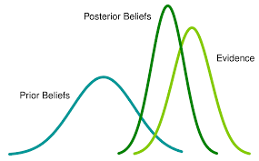
In some respects the Bayesian formulation is the simpler and in other respects the more difficult. Once a likelihood and a prior are specified to a reasonable approximation all problems are, in principle at least, straightforward. The resulting posterior distribution can be manipulated in accordance with the ordinary laws of probability. The difficulties centre on the concepts underlying the definition of the probabilities involved and then on the numerical specification of the prior to sufficient accuracy.

Sometimes, as in certain genetical problems, it is reasonable to think of $\theta$ as generated by a stochastic mechanism. There is no dispute that the Bayesian approach is at least part of a reasonable formulation and solution in such situations. In other cases to use the formulation in a literal way we have to regard probability as measuring uncertainty in a sense not necessarily directly linked to frequencies. We return to this issue later. Another possible justification of some Bayesian methods is that they provide an algorithm for extracting from the likelihood some procedures whose fundamental strength comes from frequentist considerations. This can be regarded, in particular, as supporting
$5.2$ Broad roles of probability
a broad class of procedures, known as shrinkage methods, including ridge regression.

The emphasis in this book is quite often on the close relation between answers possible from different approaches. This does not imply that the different views never conflict. Also the differences of interpretation between different numerically similar answers may be conceptually important.

统计代写|统计推断作业代写statistics interference代考|Broad roles of probability

A recurring theme in the discussion so far has concerned the broad distinction between the frequentist and the Bayesian formalization and meaning of probability. Kolmogorov’s axiomatic formulation of the theory of probability largely decoupled the issue of meaning from the mathematical aspects; his axioms were, however, firmly rooted in a frequentist view, although towards the end of his life he became concerned with a different interpretation based on complexity. But in the present context meaning is crucial.

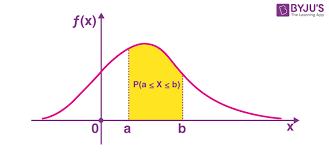
There are two ways in which probability may be used in statistical discussions. The first is phenomenological, to describe in mathematical form the empirical regularities that characterize systems containing haphazard variation. This typically underlies the formulation of a probability model for the data, in particular leading to the unknown parameters which are regarded as a focus of interest. The probability of an event $\mathcal{E}$ is an idealized limiting proportion of times in which $\mathcal{E}$ occurs in a large number of repeat observations on the system under the same conditions. In some situations the notion of a large number of repetitions can be reasonably closely realized; in others, as for example with economic time series, the notion is a more abstract construction. In both cases the working assumption is that the parameters describe features of the underlying data-generating process divorced from special essentially accidental features of the data under analysis.

That first phenomenological notion is concerned with describing variability. The second role of probability is in connection with uncertainty and is thus epistemological. In the frequentist theory we adapt the frequency-based view of probability, using it only indirectly to calibrate the notions of confidence intervals and significance tests. In most applications of the Bayesian view we need an extended notion of probability as measuring the uncertainty of $\mathcal{E}$ given $\mathcal{F}$, where now $\mathcal{E}$, for example, is not necessarily the outcome of a random system, but may be a hypothesis or indeed any feature which is unknown to the investigator. In statistical applications $\mathcal{E}$ is typically some statement about the unknown parameter $\theta$ or more specifically about the parameter of interest $\psi$. The present

discussion is largely confined to such situations. The issue of whether a single number could usefully encapsulate uncertainty about the correctness of, say, the Fundamental Theory underlying particle physics is far outside the scope of the present discussion. It could, perhaps, be applied to a more specific question such as a prediction of the Fundamental Theory: will the Higgs boson have been discovered by 2010 ?

One extended notion of probability aims, in particular, to address the point that in interpretation of data there are often sources of uncertainty additional to those arising from narrow-sense statistical variability. In the frequentist approach these aspects, such as possible systematic errors of measurement, are addressed qualitatively, usually by formal or informal sensitivity analysis, rather than incorporated into a probability assessment.

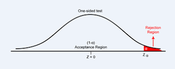
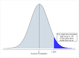
统计代写|统计推断作业代写statistics interference代考|Frequentist interpretation of upper limits

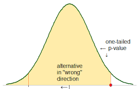
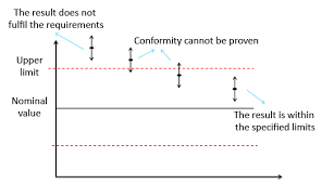
First we consider the frequentist interpretation of upper limits obtained, for example, from a suitable pivot. We take the simplest example, Example 1.1, namely the normal mean when the variance is known, but the considerations are fairly general. The upper limit
$$
\bar{y}+k_{c}^{} \sigma_{0} / \sqrt{n}, $$ derived here from the probability statement $$ P\left(\mu<\bar{Y}+k_{c}^{} \sigma_{0} / \sqrt{n}\right)=1-c,
$$
is a particular instance of a hypothetical long run of statements a proportion $1-c$ of which will be true, always, of course, assuming our model is sound. We can, at least in principle, make such a statement for each $c$ and thereby generate a collection of statements, sometimes called a confidence distribution. There is no restriction to a single $c$, so long as some compatibility requirements hold.
Because this has the formal properties of a distribution for $\mu$ it was called by R. A. Fisher the fiducial distribution and sometimes the fiducial probability distribution. A crucial question is whether this distribution can be interpreted and manipulated like an ordinary probability distribution. The position is:

a single set of limits for $\mu$ from some data can in some respects be considered just like a probability statement for $\mu$;
such probability statements cannot in general be combined or manipulated by the laws of probability to evaluate, for example, the chance that $\mu$ exceeds some given constant, for example zero. This is clearly illegitimate in the present context.

That is, as a single statement a $1-c$ upper limit has the evidential force of a statement of a unique event within a probability system. But the rules for manipulating probabilities in general do not apply. The limits are, of course, directly based on probability calculations.

Nevertheless the treatment of the confidence interval statement about the parameter as if it is in some respects like a probability statement contains the important insights that, in inference for the normal mean, the unknown parameter is more likely to be near the centre of the interval than near the end-points and that, provided the model is reasonably appropriate, if the mean is outside the interval it is not likely to be far outside.

A more emphatic demonstration that the sets of upper limits defined in this way do not determine a probability distribution is to show that in general there is an inconsistency if such a formal distribution determined in one stage of analysis is used as input into a second stage of probability calculation. We shall not give details; see Note 5.2.

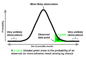
The following example illustrates in very simple form the care needed in passing from assumptions about the data, given the model, to inference about the model, given the data, and in particular the false conclusions that can follow from treating such statements as probability statements.

属性数据分析

统计代写|统计推断作业代写statistics interference代考|General remarks

我们现在可以考虑制定和比较不同方法所涉及的一些问题。

在某些方面，贝叶斯公式更简单，而在其他方面则更困难。一旦将可能性和先验指定为合理的近似值，所有问题至少在原则上都是直截了当的。由此产生的后验分布可以根据普通的概率定律进行操作。困难集中在所涉及的概率定义背后的概念上，然后是足够准确度的先验数值规范。

有时，就像在某些遗传问题中一样，有理由认为θ由随机机制产生。毫无疑问，贝叶斯方法至少是在这种情况下合理制定和解决方案的一部分。在其他情况下，要以字面的方式使用该公式，我们必须将概率视为在某种意义上测量不确定性，不一定与频率直接相关。我们稍后会回到这个问题。一些贝叶斯方法的另一个可能的理由是它们提供了一种算法，用于从可能性中提取一些基本优势来自频率论考虑的过程。这尤其可以被视为支持
5.2概率
的广泛作用一类广泛的程序，称为收缩方法，包括岭回归。

本书的重点往往是不同方法可能得出的答案之间的密切关系。这并不意味着不同的观点永远不会冲突。此外，不同数值相似答案之间的解释差异在概念上可能很重要。

统计代写|统计推断作业代写statistics interference代考|Broad roles of probability

到目前为止，讨论中反复出现的主题涉及频率论和贝叶斯形式化之间的广泛区别以及概率的含义。Kolmogorov 对概率论的公理化表述在很大程度上将意义问题与数学方面脱钩了。然而，他的公理坚定地植根于频率论观点，尽管在他生命的最后阶段，他开始关注基于复杂性的不同解释。但在目前的语境中，意义是至关重要的。

有两种方法可以在统计讨论中使用概率。第一个是现象学的，以数学形式描述表征包含随意变化的系统的经验规律。这通常是数据概率模型制定的基础，特别是导致被视为关注焦点的未知参数。事件的概率和是一个理想化的极限比例，其中和发生在相同条件下对系统的大量重复观察中。在某些情况下，可以合理地接近地实现大量重复的概念；在其他情况下，例如经济时间序列，这个概念是一个更抽象的结构。在这两种情况下，工作假设是参数描述了底层数据生成过程的特征，与所分析数据的特殊本质上的偶然特征相分离。

第一个现象学概念与描述可变性有关。概率的第二个作用与不确定性有关，因此是认识论的。在频率论理论中，我们采用基于频率的概率观点，仅间接使用它来校准置信区间和显着性检验的概念。在贝叶斯观点的大多数应用中，我们需要一个扩展的概率概念来衡量不确定性和给定F, 现在在哪里和例如，不一定是随机系统的结果，而可能是一个假设，或者实际上是调查人员不知道的任何特征。在统计应用中和通常是关于未知参数的一些陈述θ或更具体地说，关于感兴趣的参数ψ. 现在

讨论主要限于这种情况。单个数字是否可以有效地封装关于粒子物理学基础理论正确性的不确定性的问题远远超出了本讨论的范围。也许，它可以应用于更具体的问题，例如对基本理论的预测：到 2010 年会发现希格斯玻色子吗？

一个扩展的概率概念旨在解决这一点，即在解释数据时，除了狭义统计可变性引起的不确定性之外，还经常存在不确定性来源。在频率论方法中，这些方面，例如可能的系统测量误差，通常通过正式或非正式的敏感性分析来定性地解决，而不是纳入概率评估中。

统计代写|统计推断作业代写statistics interference代考|Frequentist interpretation of upper limits

首先，我们考虑例如从合适的支点获得的上限的常客解释。我们采用最简单的例子，例 1.1，即方差已知时的正态均值，但考虑相当普遍。上限
是¯+到Cσ0/n,这里从概率陈述中得出磷(μ<是¯+到Cσ0/n)=1−C,
是假设的长期陈述的特定实例比例1−C当然，假设我们的模型是合理的，这将是正确的。至少在原则上，我们可以为每个C从而生成一组语句，有时称为置信度分布。没有单一的限制C，只要一些兼容性要求成立。
因为这具有分布的形式属性μRA Fisher 将其称为基准分布，有时也称为基准概率分布。一个关键问题是这个分布是否可以像普通概率分布一样被解释和操纵。职位是：

一组限制μ从某些数据中可以在某些方面被认为就像一个概率陈述μ;
这种概率陈述通常不能被概率法则组合或操纵来评估，例如，μ超过某个给定的常数，例如零。在目前的情况下，这显然是非法的。

也就是说，作为一个单一的陈述1−C上限具有陈述概率系统中唯一事件的证据力。但一般来说，操纵概率的规则并不适用。当然，这些限制直接基于概率计算。

然而，将关于参数的置信区间陈述视为在某些方面类似于概率陈述的处理包含了重要的见解，即在推断正态均值时，未知参数更可能靠近区间中心而不是接近端点，并且只要模型合理合适，如果平均值在区间之外，它不太可能在区间之外很远。

以这种方式定义的上限集合并不能确定概率分布的更强有力的证明是表明，如果将在一个分析阶段确定的正式分布用作第二阶段的输入，则通常存在不一致。概率计算。我们不会提供细节；见注 5.2。

以下示例以非常简单的形式说明了从对数据的假设（给定模型）到对模型的推断（给定数据）所需的谨慎，特别是通过将此类陈述视为概率陈述可能得出的错误结论。

统计代写|统计推断作业代写statistics interference代考请认准statistics-lab™

统计代写请认准statistics-lab™. statistics-lab™为您的留学生涯保驾护航。统计代写|python代写代考

随机过程代考

在概率论概念中，随机过程是随机变量的集合。若一随机系统的样本点是随机函数，则称此函数为样本函数，这一随机系统全部样本函数的集合是一个随机过程。实际应用中，样本函数的一般定义在时间域或者空间域。 随机过程的实例如股票和汇率的波动、语音信号、视频信号、体温的变化，随机运动如布朗运动、随机徘徊等等。

贝叶斯方法代考

贝叶斯统计概念及数据分析表示使用概率陈述回答有关未知参数的研究问题以及统计范式。后验分布包括关于参数的先验分布，和基于观测数据提供关于参数的信息似然模型。根据选择的先验分布和似然模型，后验分布可以解析或近似，例如，马尔科夫链蒙特卡罗 (MCMC) 方法之一。贝叶斯统计概念及数据分析使用后验分布来形成模型参数的各种摘要，包括点估计，如后验平均值、中位数、百分位数和称为可信区间的区间估计。此外，所有关于模型参数的统计检验都可以表示为基于估计后验分布的概率报表。

广义线性模型代考

广义线性模型（GLM）归属统计学领域，是一种应用灵活的线性回归模型。该模型允许因变量的偏差分布有除了正态分布之外的其它分布。

statistics-lab作为专业的留学生服务机构，多年来已为美国、英国、加拿大、澳洲等留学热门地的学生提供专业的学术服务，包括但不限于Essay代写，Assignment代写，Dissertation代写，Report代写，小组作业代写，Proposal代写，Paper代写，Presentation代写，计算机作业代写，论文修改和润色，网课代做，exam代考等等。写作范围涵盖高中，本科，研究生等海外留学全阶段，辐射金融，经济学，会计学，审计学，管理学等全球99%专业科目。写作团队既有专业英语母语作者，也有海外名校硕博留学生，每位写作老师都拥有过硬的语言能力，专业的学科背景和学术写作经验。我们承诺100%原创，100%专业，100%准时，100%满意。

机器学习代写

随着AI的大潮到来，Machine Learning逐渐成为一个新的学习热点。同时与传统CS相比，Machine Learning在其他领域也有着广泛的应用，因此这门学科成为不仅折磨CS专业同学的“小恶魔”，也是折磨生物、化学、统计等其他学科留学生的“大魔王”。学习Machine learning的一大绊脚石在于使用语言众多，跨学科范围广，所以学习起来尤其困难。但是不管你在学习Machine Learning时遇到任何难题，StudyGate专业导师团队都能为你轻松解决。

多元统计分析代考

基础数据: $N$ 个样本， $P$ 个变量数的单样本，组成的横列的数据表
变量定性: 分类和顺序；变量定量：数值
数学公式的角度分为: 因变量与自变量

时间序列分析代写

随机过程，是依赖于参数的一组随机变量的全体，参数通常是时间。随机变量是随机现象的数量表现，其时间序列是一组按照时间发生先后顺序进行排列的数据点序列。通常一组时间序列的时间间隔为一恒定值（如1秒，5分钟，12小时，7天，1年），因此时间序列可以作为离散时间数据进行分析处理。研究时间序列数据的意义在于现实中，往往需要研究某个事物其随时间发展变化的规律。这就需要通过研究该事物过去发展的历史记录，以得到其自身发展的规律。

回归分析代写

多元回归分析渐进（Multiple Regression Analysis Asymptotics）属于计量经济学领域，主要是一种数学上的统计分析方法，可以分析复杂情况下各影响因素的数学关系，在自然科学、社会和经济学等多个领域内应用广泛。

MATLAB代写

MATLAB 是一种用于技术计算的高性能语言。它将计算、可视化和编程集成在一个易于使用的环境中，其中问题和解决方案以熟悉的数学符号表示。典型用途包括：数学和计算算法开发建模、仿真和原型制作数据分析、探索和可视化科学和工程图形应用程序开发，包括图形用户界面构建MATLAB 是一个交互式系统，其基本数据元素是一个不需要维度的数组。这使您可以解决许多技术计算问题，尤其是那些具有矩阵和向量公式的问题，而只需用 C 或 Fortran 等标量非交互式语言编写程序所需的时间的一小部分。MATLAB 名称代表矩阵实验室。MATLAB 最初的编写目的是提供对由 LINPACK 和 EISPACK 项目开发的矩阵软件的轻松访问，这两个项目共同代表了矩阵计算软件的最新技术。MATLAB 经过多年的发展，得到了许多用户的投入。在大学环境中，它是数学、工程和科学入门和高级课程的标准教学工具。在工业领域，MATLAB 是高效研究、开发和分析的首选工具。MATLAB 具有一系列称为工具箱的特定于应用程序的解决方案。对于大多数 MATLAB 用户来说非常重要，工具箱允许您学习和应用专业技术。工具箱是 MATLAB 函数（M 文件）的综合集合，可扩展 MATLAB 环境以解决特定类别的问题。可用工具箱的领域包括信号处理、控制系统、神经网络、模糊逻辑、小波、仿真等。

R语言代写	问卷设计与分析代写
PYTHON代写	回归分析与线性模型代写
MATLAB代写	方差分析与试验设计代写
STATA代写	机器学习/统计学习代写
SPSS代写	计量经济学代写
EVIEWS代写	时间序列分析代写
EXCEL代写	深度学习代写
SQL代写	各种数据建模与可视化代写

统计代写|统计推断作业代写statistics interference代考|Some more general frequentist developments

Posted on 2022年4月14日2022年4月14日 by statistics-lab

如果你也在怎样代写统计推断statistics interference这个学科遇到相关的难题，请随时右上角联系我们的24/7代写客服。

统计推断是利用数据分析来推断概率基础分布的属性的过程。推断性统计分析推断人口的属性，例如通过测试假设和得出估计值。

我们提供的属性统计推断statistics interference及其相关学科的代写，服务范围广, 其中包括但不限于:

Statistical Inference 统计推断
Statistical Computing 统计计算
Advanced Probability Theory 高等楖率论
Advanced Mathematical Statistics 高等数理统计学
(Generalized) Linear Models 广义线性模型
Statistical Machine Learning 统计机器学习
Longitudinal Data Analysis 纵向数据分析
Foundations of Data Science 数据科学基础

Bayesian inference - Wikipedia — 统计代写|统计推断作业代写statistics interference代考|Some more general frequentist developments

统计代写|统计推断作业代写statistics interference代考|Exponential family problems

Some limited but important classes of problems have a formally exact solution within the frequentist approach. We begin with two situations involving exponential family distributions. For simplicity we suppose that the parameter $\psi$ of interest is one-dimensional.

We start with a full exponential family model in which $\psi$ is a linear combination of components of the canonical parameter. After linear transformation of the parameter and canonical statistic we can write the density of the observations in the form
$$
m(y) \exp \left{s_{\psi} \psi+s_{\lambda}^{T} \lambda-k(\psi, \lambda)\right}
$$
where $\left(s_{\psi}, s_{\lambda}\right)$ is a partitioning of the sufficient statistic corresponding to the partitioning of the parameter. For inference about $\psi$ we prefer a pivotal distribution not depending on $\lambda$. It can be shown via the mathematical property of completeness, essentially that the parameter space is rich enough, that separation from $\lambda$ can be achieved only by working with the conditional distribution of the data given $S_{\lambda}=s_{\lambda}$. That is, we evaluate the conditional distribution of $S_{\psi}$ given $S_{\lambda}=s_{\lambda}$ and use the resulting distribution to find which values of $\psi$ are consistent with the data at various levels.

Many of the standard procedures dealing with simple problems about Poisson, binomial, gamma and normal distributions can be found by this route.We illustrate the arguments sketched above by a number of problems connected with binomial distributions, noting that the canonical parameter of a binomial distribution with probability $\pi$ is $\phi=\log {\pi /(1-\pi)}$. This has some advantages in interpretation and also disadvantages. When $\pi$ is small, the parameter is essentially equivalent to $\log \pi$ meaning that differences in canonical parameter are equivalent to ratios of probabilities.

统计代写|统计推断作业代写statistics interference代考|Transformation models

A different kind of reduction is possible for models such as the location model which preserve a special structure under a family of transformations.

Example 4.10. Location model. We return to Example 1.8, the location model. The likelihood is $\Pi g\left(y_{k}-\mu\right)$ which can be rearranged in terms of the order statistics $y_{(t)}$, i.e., the observed values arranged in increasing order of magnitude. These in general form the sufficient statistic for the model, minimal except for the normal distribution. Now the random variables corresponding to the differences between order statistics, specified, for example, as
$$
a=\left(y_{(2)}-y_{(1)}, \ldots, y_{(n)}-y_{(1)}\right)=\left(a_{2}, \ldots, a_{n}\right),
$$
have a distribution not depending on $\mu$ and hence are ancillary; inference about $\mu$ is thus based on the conditional distribution of, say, $y_{(1)}$ given $A=a$. The choice of $y_{(1)}$ is arbitrary because any estimate of location, for example the mean, is $y_{(1)}$ plus a function of $a$, and the latter is not random after conditioning. Now the marginal density of $A$ is
$$
\int g\left(y_{(1)}-\mu\right) g\left(y_{(1)}+a_{2}-\mu\right) \cdots g\left(y_{(1)}+a_{n}-\mu\right) d y_{(1)} .
$$The integral with respect to $y_{(1)}$ is equivalent to one integrated with respect to $\mu$ so that, on reexpressing the integrand in terms of the likelihood for the unordered variables, the density of $A$ is the function necessary to normalize the likelihood to integrate to one with respect to $\mu$. That is, the conditional density of $Y_{(1)}$, or of any other measure of location, is determined by normalizing the likelihood function and regarding it as a function of $y_{(1)}$ for given $a$. This implies that $p$-values and confidence limits for $\mu$ result from normalizing the likelihood and treating it like a distribution of $\mu$.

This is an exceptional situation in frequentist theory. In general, likelihood is a point function of its argument and integrating it over sets of parameter values is not statistically meaningful. In a Bayesian formulation it would correspond to combination with a uniform prior but no notion of a prior distribution is involved in the present argument.

The ancillary statistics allow testing conformity with the model. For example, to check on the functional form of $g(.)$ it would be best to work with the differences of the ordered values from the mean, $\left(y_{(l)}-\bar{y}\right)$ for $l=1, \ldots, n$. These are functions of $a$ as previously defined. A test statistic could be set up informally sensitive to departures in distributional form from those implied by $g(.)$. Or $\left(y_{(l)}-\bar{y}\right)$ could be plotted against $G^{-1}{(l-1 / 2) /(n+1)}$, where $G(.)$ is the cumulative distribution function corresponding to the density $g(.)$.

统计代写|统计推断作业代写statistics interference代考|Some further Bayesian examples

In principle the prior density in a Bayesian analysis is an insertion of additional information and the form of the prior should be dictated by the nature of that evidence. It is useful, at least for theoretical discussion, to look at priors which lead to mathematically tractable answers. One such form, useful usually only for nuisance parameters, is to take a distribution with finite support, in particular a two-point prior. This has in one dimension three adjustable parameters, the position of two points and a probability, and for some limited purposes this may be adequate. Because the posterior distribution remains concentrated on the same two points computational aspects are much simplified.

We shall not develop that idea further and turn instead to other examples of parametric conjugate priors which exploit the consequences of exponential family structure as exemplified in Section 2.4.

Example 4.12. Normal variance. Suppose that $Y_{1}, \ldots, Y_{n}$ are independently normally distributed with known mean, taken without loss of generality to be zero, and unknown variance $\sigma^{2}$. The likelihood is, except for a constant factor,
$$
\frac{1}{\sigma^{n}} \exp \left{-\Sigma y_{k}^{2} /\left(2 \sigma^{2}\right)\right} .
$$
The canonical parameter is $\phi=1 / \sigma^{2}$ and simplicity of structure suggests taking $\phi$ to have a prior gamma density which it is convenient to write in the form
$$
\pi\left(\phi ; g, n_{\pi}\right)=g(g \phi)^{n_{\pi} / 2-1} e^{-g \phi} / \Gamma\left(n_{\pi} / 2\right),
$$

defined by two quantities assumed known. One is $n_{\pi}$, which plays the role of an effective sample size attached to the prior density, by analogy with the form of the chi-squared density with $n$ degrees of freedom. The second defining quantity is $g$. Transformed into a distribution for $\sigma^{2}$ it is often called the inverse gamma distribution. Also $E_{\pi}(\Phi)=n_{\pi} /(2 g)$.

On multiplying the likelihood by the prior density, the posterior density of $\Phi$ is proportional to
$$
\phi^{\left(n+n_{\pi}\right) / 2-1} \exp \left[-\left{\left(\Sigma y_{k}^{2}+n_{\pi} / E_{\pi}(\Phi)\right)\right} \phi / 2\right]
$$
The posterior distribution is in effect found by treating
$$
\left{\Sigma y_{k}^{2}+n_{\pi} / E_{\pi}(\Phi)\right} \Phi
$$
as having a chi-squared distribution with $n+n_{\pi}$ degrees of freedom.
Formally, frequentist inference is based on the pivot $\Sigma Y_{k}^{2} / \sigma^{2}$, the pivotal distribution being the chi-squared distribution with $n$ degrees of freedom. There is formal, although of course not conceptual, equivalence between the two methods when $n_{a}=0$. This arises from the improper prior $d \phi / \phi$, equivalent to $d \sigma / \sigma$ or to a uniform improper prior for $\log \sigma$. That is, while there is never in this setting exact agreement between Bayesian and frequentist solutions, the latter can be approached as a limit as $n_{\pi} \rightarrow 0$.

统计代写|统计推断作业代写statistics interference代考|Some more general frequentist developments

属性数据分析

统计代写|统计推断作业代写statistics interference代考|Exponential family problems

一些有限但重要的问题类别在频率论方法中具有形式上精确的解决方案。我们从涉及指数族分布的两种情况开始。为简单起见，我们假设感兴趣的参数是一维的。

我们从一个完整的指数族模型开始，其中是规范参数分量的线性组合。在参数和典型统计量的线性变换之后，我们可以将观测值的密度写成以下形式
m(y) \exp \left{s_{\psi} \psi+s_{\lambda}^{T} \lambda-k(\psi, \lambda)\right}

其中是对应于参数划分的充分统计量的划分。对于推断，我们更喜欢不依赖于的关键分布。可以通过完备性的数学性质表明，本质上参数空间足够丰富，只有通过给定数据的条件分布才能实现分离。也就是说，我们评估给定的条件分布，并使用结果分布来找出哪些值与各个级别的数据一致。

许多处理有关泊松、二项式、伽马和正态分布的简单问题的标准程序都可以通过这条路线找到。我们通过与二项式分布相关的一些问题来说明上面概述的论点，注意到二项式分布的规范参数概率是。这在解释上有一些优点，也有一些缺点。当较小时，参数本质上等同于规范参数的差异等同于概率比的意思。

统计代写|统计推断作业代写statistics interference代考|Transformation models

对于诸如位置模型这样的模型可以进行不同类型的归约，该模型在一系列变换下保留了特殊结构。

示例 4.10。定位模型。我们回到示例 1.8，位置模型。可能性是 $\Pi g\left(y_{k}-\mu\right)$，它可以根据顺序统计 $y_{(t)}$ 重新排列，即观察值按递增顺序排列震级。这些通常构成模型的足够统计量，除了正态分布之外是最小的。现在将随机变量对应的订单统计量的差异，指定为例如
$$
a=\left(y_{(2)}-y_{(1)}, \ldots, y_{ (n)}-y_{(1)}\right)=\left(a_{2}, \ldots, a_{n}\right),
$$
有一个不依赖于 $\ 的分布mu$，因此是辅助的；因此，关于 $\mu$ 的推断是基于给定 $A=a$ 的 $y_{(1)}$ 的条件分布。 $y_{(1)}$ 的选择是任意的，因为任何位置估计，例如均值，都是 $y_{(1)}$ 加上 $a$ 的函数，而后者在调节后不是随机的。现在$A$的边际密度是
$$
\int g\left(y_{(1)}-\mu\right) g\left(y_{(1)}+a_{2} -\mu\right) \cdots g\left(y_{(1)}+a_{n}-\mu\right) d y_{(1)} .
$$关于$y_{的积分(1)}$ 等价于关于 $\mu$ 的积分，因此，在根据无序变量的似然性重新表示被积函数时，$A$ 的密度是归一化似然性所必需的函数对于 $\mu$ 为一。也就是说，$Y_{(1)}$ 或任何其他位置度量的条件密度是通过对似然函数进行归一化并将其视为给定 $a 的 $y_{(1)}$ 的函数来确定的美元。这意味着 $\mu$ 的 $p$ 值和置信限来自于对可能性进行归一化并将其视为 $\mu$ 的分布。

对于诸如位置模型这样的模型可以进行不同类型的归约，该模型在一系列变换下保留了特殊结构。

示例 4.10。定位模型。我们回到示例 1.8，位置模型。可能性是 $\Pi g\left(y_{k}-\mu\right)$，它可以根据顺序统计 $y_{(t)}$ 重新排列，即观察值按递增顺序排列震级。这些通常构成模型的足够统计量，除了正态分布之外是最小的。现在将随机变量对应的订单统计量的差异，指定为例如

$$
a=\left(y_{(2)}-y_{(1)}, \ldots, y_{ (n)}-y_{(1)}\right)=\left(a_{2}, \ldots, a_{n}\right),
$$
有一个不依赖于 $\ 的分布mu$，因此是辅助的；因此，关于 $\mu$ 的推断是基于给定 $A=a$ 的 $y_{(1)}$ 的条件分布。 $y_{(1)}$ 的选择是任意的，因为任何位置估计，例如均值，都是 $y_{(1)}$ 加上 $a$ 的函数，而后者在调节后不是随机的。现在$A$的边际密度是
$$
\int g\left(y_{(1)}-\mu\right) g\left(y_{(1)}+a_{2} -\mu\right) \cdots g\left(y_{(1)}+a_{n}-\mu\right) d y_{(1)} .
$$关于$y_{的积分(1)}$ 等价于关于 $\mu$ 的积分，因此，在根据无序变量的似然性重新表示被积函数时，$A$ 的密度是归一化似然性所必需的函数对于 $\mu$ 为一。也就是说，$Y_{(1)}$ 或任何其他位置度量的条件密度是通过对似然函数进行归一化并将其视为给定 $a 的 $y_{(1)}$ 的函数来确定的美元。这意味着 $\mu$ 的 $p$ 值和置信限来自于对可能性进行归一化并将其视为 $\mu$ 的分布。

辅助统计数据允许测试与模型的一致性。例如，要检查 $g(.)$ 的函数形式，最好使用有序值与平均值的差异 $\left(y_{(l)}-\bar{y}\对)$ 为 $l=1, \ldots, n$。这些是前面定义的 $a$ 的函数。可以非正式地建立一个检验统计量，以对分布形式与 $g(.)$ 隐含的偏差敏感。或者 $\left(y_{(l)}-\bar{y}\right)$ 可以针对 $G^{-1}{(l-1 / 2) /(n+1)}$ 绘制，其中$G(.)$是密度$g(.)$对应的累积分布函数。

这是频率论中的一个例外情况。一般而言，似然度是其参数的点函数，将其集成到参数值集上没有统计意义。在贝叶斯公式中，它对应于与统一先验的组合，但本论点不涉及先验分布的概念。

统计代写|统计推断作业代写statistics interference代考|Some further Bayesian examples

我们不会进一步发展这个想法，而是转向参数共轭先验的其他示例，这些示例利用指数族结构的后果，如第 2.4 节所示。

示例 4.12。正常方差。假设 $Y_{1}、\ldots、Y_{n}$ 独立正态分布，均值已知，不失一般性取为零，方差未知 $\sigma^{2}$。可能性是，除了一个常数因子，
$$
\frac{1}{\sigma^{n}} \exp \left{-\Sigma y_{k}^{2} /\left (2 \sigma^{2}\right)\right} .
$$
规范参数是 $\phi=1 / \sigma^{2}$，结构简单建议取 $\phi$有一个先验的伽马密度，可以方便地写成
$$
\pi\left(\phi ; g, n_{\pi}\right)=g(g \phi)^{ n_{\pi} / 2-1} e^{-g \phi} / \Gamma\left(n_{\pi} / 2\right),
$$

原则上，贝叶斯分析中的先验密度是附加信息的插入，先验的形式应由该证据的性质决定。至少对于理论讨论而言，查看导致数学上易于处理的答案的先验是有用的。一种这样的形式，通常只对讨厌的参数有用，是采用有限支持的分布，特别是两点先验。这在一维中具有三个可调整的参数、两个点的位置和一个概率，对于某些有限的目的，这可能就足够了。因为后验分布仍然集中在相同的两点上，所以计算方面大大简化了。

我们不会进一步发展这个想法，而是转向参数共轭先验的其他示例，这些示例利用指数族结构的后果，如第 2.4 节所示。

示例 4.12。正常方差。假设 $Y_{1}、\ldots、Y_{n}$ 独立正态分布，均值已知，不失一般性取为零，方差未知 $\sigma^{2}$。可能性是，除了一个常数因子，

$$
\frac{1}{\sigma^{n}} \exp \left{-\Sigma y_{k}^{2} /\left (2 \sigma^{2}\right)\right} .
$$
规范参数是 $\phi=1 / \sigma^{2}$，结构简单建议取 $\phi$有一个先验的伽马密度，可以方便地写成
$$
\pi\left(\phi ; g, n_{\pi}\right)=g(g \phi)^{ n_{\pi} / 2-1} e^{-g \phi} / \Gamma\left(n_{\pi} / 2\right),
$$原则上，贝叶斯分析中的先验密度是附加信息的插入，先验的形式应由该证据的性质决定。至少对于理论讨论而言，查看导致数学上易于处理的答案的先验是有用的。一种这样的形式，通常只对讨厌的参数有用，是采用有限支持的分布，特别是两点先验。这在一维中具有三个可调整的参数、两个点的位置和一个概率，对于某些有限的目的，这可能就足够了。因为后验分布仍然集中在相同的两点上，所以计算方面大大简化了。

我们不会进一步发展这个想法，而是转向参数共轭先验的其他示例，这些示例利用指数族结构的后果，如第 2.4 节所示。示例 4.12。正常方差。假设 $Y_{1}、\ldots、Y_{n}$ 独立正态分布，均值已知，不失一般性取为零，方差未知 $\sigma^{2}$。可能性是，除了一个常数因子，

由假定已知的两个量定义。一个是$n_{\pi}$，它起到了附加到先验密度的有效样本大小的作用，类似于具有$n$自由度的卡方密度的形式。第二个定义量是$g$。转换为 $\sigma^{2}$ 的分布，它通常被称为逆伽马分布。还有$E_{\pi}(\Phi)=n_{\pi} /(2 g)$。

在将似然乘以先验密度时，$\Phi$ 的后验密度与
$$
\phi^{\left(n+n_{\pi}\right) / 2 成正比-1} \exp \left[-\left{\left(\Sigma y_{k}^{2}+n_{\pi} / E_{\pi}(\Phi)\right)\right} \phi / 2\right]
$$
后验分布实际上是通过处理
$$
\left{\Sigma y_{k}^{2}+n_{\pi} / E_ {\pi}(\Phi)\right} \Phi
$$
具有 $n+n_{\pi}$ 自由度的卡方分布。
形式上，频率论推理是基于枢轴 $\Sigma Y_{k}^{2} / \sigma^{2}$，枢轴分布是具有 $n$ 自由度的卡方分布。当 $n_{a}=0$ 时，两种方法之间存在形式上的等价，当然不是概念上的等价。这是由不正确的先验$d \phi / \phi$ 引起的，相当于$d \sigma / \sigma$ 或$\log \sigma$ 的统一不正确的先验。也就是说，虽然在这种情况下，贝叶斯和常客解决方案之间从来没有完全一致，但后者可以作为 $n_{\pi} \rightarrow 0$ 的限制来接近。

在将似然乘以先验密度时，$\Phi$ 的后验密度与

$$
\phi^{\left(n+n_{\pi}\right) / 2 成正比-1} \exp \left[-\left{\left(\Sigma y_{k}^{2}+n_{\pi} / E_{\pi}(\Phi)\right)\right} \phi / 2\right]
$$
后验分布实际上是通过处理
$$
\left{\Sigma y_{k}^{2}+n_{\pi} / E_ {\pi}(\Phi)\right} \Phi
$$
具有 $n+n_{\pi}$ 自由度的卡方分布。
形式上，频率论推理是基于枢轴 $\Sigma Y_{k}^{2} / \sigma^{2}$，枢轴分布是具有 $n$ 自由度的卡方分布。当 $n_{a}=0$ 时，两种方法之间存在形式上的等价，当然不是概念上的等价。这是由不正确的先验$d \phi / \phi$ 引起的，相当于$d \sigma / \sigma$ 或$\log \sigma$ 的统一不正确的先验。也就是说，虽然在这种情况下，贝叶斯和常客解决方案之间从来没有完全一致，但后者可以作为 $n_{\pi} \rightarrow 0$ 的限制来接近。

统计代写请认准statistics-lab™. statistics-lab™为您的留学生涯保驾护航。统计代写|python代写代考

随机过程代考

贝叶斯方法代考

广义线性模型代考

广义线性模型（GLM）归属统计学领域，是一种应用灵活的线性回归模型。该模型允许因变量的偏差分布有除了正态分布之外的其它分布。

机器学习代写

多元统计分析代考

基础数据: $N$ 个样本， $P$ 个变量数的单样本，组成的横列的数据表
变量定性: 分类和顺序；变量定量：数值
数学公式的角度分为: 因变量与自变量

时间序列分析代写

回归分析代写

MATLAB代写

R语言代写	问卷设计与分析代写
PYTHON代写	回归分析与线性模型代写
MATLAB代写	方差分析与试验设计代写
STATA代写	机器学习/统计学习代写
SPSS代写	计量经济学代写
EVIEWS代写	时间序列分析代写
EXCEL代写	深度学习代写
SQL代写	各种数据建模与可视化代写

统计代写|统计推断作业代写statistics interference代考|More complicated situations

Posted on 2022年4月14日2022年4月14日 by statistics-lab

如果你也在怎样代写统计推断statistics interference这个学科遇到相关的难题，请随时右上角联系我们的24/7代写客服。

统计推断是利用数据分析来推断概率基础分布的属性的过程。推断性统计分析推断人口的属性，例如通过测试假设和得出估计值。

我们提供的属性统计推断statistics interference及其相关学科的代写，服务范围广, 其中包括但不限于:

Statistical Inference 统计推断
Statistical Computing 统计计算
Advanced Probability Theory 高等楖率论
Advanced Mathematical Statistics 高等数理统计学
(Generalized) Linear Models 广义线性模型
Statistical Machine Learning 统计机器学习
Longitudinal Data Analysis 纵向数据分析
Foundations of Data Science 数据科学基础

统计代写|统计推断作业代写statistics interference代考|More complicated situations

统计代写|统计推断作业代写statistics interference代考|General remarks

The previous frequentist discussion in especially Chapter 3 yields a theoretical approach which is limited in two senses. It is restricted to problems with no nuisance parameters or ones in which elimination of nuisance parameters is straightforward. An important step in generalizing the discussion is to extend the notion of a Fisherian reduction. Then we turn to a more systematic discussion of the role of nuisance parameters.

By comparison, as noted previously in Section 1.5, a great formal advantage of the Bayesian formulation is that, once the formulation is accepted, all subsequent problems are computational and the simplifications consequent on sufficiency serve only to ease calculations.

统计代写|统计推断作业代写statistics interference代考|General Bayesian formulation

The argument outlined in Section $1.5$ for inference about the mean of a normal distribution can be generalized as follows. Consider the model $f_{Y \mid \Theta}(y \mid \theta)$, where, because we are going to treat the unknown parameter as a random variable, we now regard the model for the data-generating process as a conditional density. Suppose that $\Theta$ has the prior density $f_{\Theta}(\theta)$, specifying the marginal

distribution of the parameter, i.e., in effect the distribution $\Theta$ has when the observations $y$ are not available.

Given the data and the above formulation it is reasonable to assume that all information about $\theta$ is contained in the conditional distribution of $\Theta$ given $Y=y$. We call this the posterior distribution of $\Theta$ and calculate it by the standard laws of probability theory, as given in (1.12), by
$$
f_{\Theta \mid Y}(\theta \mid y)=\frac{f_{Y \mid \Theta}(y \mid \theta) f_{\Theta}(\theta)}{\int_{\Omega_{\theta}} f_{Y \mid \Theta}(y \mid \phi) f_{\Theta}(\phi) d \phi} .
$$
The main problem in computing this lies in evaluating the normalizing constant in the denominator, especially if the dimension of the parameter space is high. Finally, to isolate the information about the parameter of interest $\psi$, we marginalize the posterior distribution over the nuisance parameter $\lambda$. That is, writing $\theta=(\psi, \lambda)$, we consider
$$
f_{\Psi \mid Y}(\psi \mid y)=\int f_{\Theta \mid Y}(\psi, \lambda \mid y) d \lambda
$$
The models and parameters for which this leads to simple explicit solutions are broadly those for which frequentist inference yields simple solutions.

Because in the formula for the posterior density the prior density enters both in the numerator and the denominator, formal multiplication of the prior density by a constant would leave the answer unchanged. That is, there is no need for the prior measure to be normalized to 1 so that, formally at least, improper, i.e. divergent, prior densities may be used, always provided proper posterior densities result. A simple example in the context of the normal mean, Section $1.5$, is to take as prior density element $f_{M}(\mu) d \mu$ just $d \mu$. This could be regarded as the limit of the proper normal prior with variance $v$ taken as $v \rightarrow \infty$. Such limits raise few problems in simple cases, but in complicated multiparameter problems considerable care would be needed were such limiting notions contemplated. There results here a posterior distribution for the mean that is normal with mean $\bar{y}$ and variance $\sigma_{0}^{2} / n$, leading to posterior limits numerically identical to confidence limits.

In fact, with a scalar parameter it is possible in some generality to find a prior giving very close agreement with corresponding confidence intervals. With multidimensional parameters this is not in general possible and naive use of flat priors can lead to procedures that are very poor from all perspectives; see Example 5.5.

统计代写|统计推断作业代写statistics interference代考|Frequentist analysis

One approach to simple problems is essentially that of Section $2.5$ and can be summarized, as before, in the Fisherian reduction:

find the likelihood function;
reduce to a sufficient statistic $S$ of the same dimension as $\theta$;
find a function of $S$ that has a distribution depending only on $\psi$;
place it in pivotal form or alternatively use it to derive $p$-values for null hypotheses;
invert to obtain limits for $\psi$ at an arbitrary set of probability levels.
There is sometimes an extension of the method that works when the model is of the $(k, d)$ curved exponential family form. Then the sufficient statistic is of dimension $k$ greater than $d$, the dimension of the parameter space. We then proceed as follows:
if possible, rewrite the $k$-dimensional sufficient statistic, when $k>d$, in the form $(S, A)$ such that $S$ is of dimension $d$ and $A$ has a distribution not depending on $\theta$;
consider the distribution of $S$ given $A=a$ and proceed as before. The statistic $A$ is called ancillary.
There are limitations to these methods. In particular a suitable A may not exist, and then one is driven to asymptotic, i.e., approximate, arguments for problems of reasonable complexity and sometimes even for simple problems.
We give some examples, the first of which is not of exponential family form.
Example 4.1. Uniform distribution of known range. Suppose that $\left(Y_{1}, \ldots, Y_{n}\right)$ are independently and identically distributed in the uniform distribution over $(\theta-1, \theta+1)$. The likelihood takes the constant value $2^{-n}$ provided the smallest

and largest values $\left(y_{(1)}, y_{(n)}\right)$ lie within the range $(\theta-1, \theta+1)$ and is zero otherwise. The minimal sufficient statistic is of dimension 2 , even though the parameter is only of dimension 1 . The model is a special case of a location family and it follows from the invariance properties of such models that $A=Y_{(n)}-Y_{(1)}$ has a distribution independent of $\theta$.

This example shows the imperative of explicit or implicit conditioning on the observed value $a$ of $A$ in quite compelling form. If $a$ is approximately 2 , only values of $\theta$ very close to $y^{}=\left(y_{(1)}+y_{(n)}\right) / 2$ are consistent with the data. If, on the other hand, $a$ is very small, all values in the range of the common observed value $y^{}$ plus and minus 1 are consistent with the data. In general, the conditional distribution of $Y^{}$ given $A=a$ is found as follows. The joint density of $\left(Y_{(1)}, Y_{(n)}\right)$ is $$ n(n-1)\left(y_{(n)}-y_{(1)}\right)^{n-2} / 2^{n} $$ and the transformation to new variables $\left(Y^{}, A=Y_{(n)}-Y_{(1)}\right)$ has unit Jacobian. Therefore the new variables $\left(Y^{}, A\right)$ have density $n(n-1) a^{(n-2)} / 2^{n}$ defined over the triangular region $\left(0 \leq a \leq 2 ; \theta-1+a / 2 \leq y^{} \leq \theta+1-a / 2\right)$ and density zero elsewhere. This implies that the conditional density of $Y^{}$ given $A=a$ is uniform over the allowable interval $\theta-1+a / 2 \leq y^{} \leq \theta+1-a / 2$.

Conditional confidence interval statements can now be constructed although they add little to the statement just made, in effect that every value of $\theta$ in the relevant interval is in some sense equally consistent with the data. The key point is that an interval statement assessed by its unconditional distribution could be formed that would give the correct marginal frequency of coverage but that would hide the fact that for some samples very precise statements are possible whereas for others only low precision is achievable.

属性数据分析

统计代写|统计推断作业代写statistics interference代考|General remarks

之前的常客讨论，尤其是第 3 章中的讨论，产生了一种在两个意义上受到限制的理论方法。它仅限于没有干扰参数的问题或消除干扰参数很简单的问题。概括讨论的一个重要步骤是扩展 Fisherian 约简的概念。然后我们转向对有害参数的作用进行更系统的讨论。

相比之下，如前面 1.5 节所述，贝叶斯公式的一个很大的形式优势是，一旦公式被接受，所有后续问题都是计算的，并且因充分性而产生的简化仅用于简化计算。

统计代写|统计推断作业代写statistics interference代考|General Bayesian formulation

节中概述的论点1.5关于正态分布均值的推断可以概括如下。考虑模型F是∣θ(是∣θ), 其中，因为我们要将未知参数视为随机变量，所以我们现在将数据生成过程的模型视为条件密度。假设θ具有先验密度Fθ(θ)，指定边际

参数的分布，即实际上分布θ有什么时候观察是不可用。

鉴于数据和上述公式，可以合理地假设所有关于θ包含在条件分布中θ给定是=是. 我们称之为后验分布θ并根据（1.12）中给出的概率论的标准定律计算它，由
Fθ∣是(θ∣是)=F是∣θ(是∣θ)Fθ(θ)∫ΩθF是∣θ(是∣φ)Fθ(φ)dφ.
计算这个的主要问题在于评估分母中的归一化常数，特别是如果参数空间的维数很高。最后，隔离有关感兴趣参数的信息ψ，我们边缘化了讨厌参数的后验分布λ. 也就是说，写θ=(ψ,λ)，我们认为
FΨ∣是(ψ∣是)=∫Fθ∣是(ψ,λ∣是)dλ
这导致简单显式解决方案的模型和参数广泛地是频率论推理产生简单解决方案的模型和参数。

因为在后验密度公式中，先验密度在分子和分母中都输入，所以先验密度乘以一个常数的形式乘法将使答案保持不变。也就是说，没有必要将先验测量归一化为1，以便至少在形式上可以使用不正确的，即发散的先验密度，总是提供适当的后验密度结果。正态均值上下文中的一个简单示例，Section1.5, 是作为先验密度元素F米(μ)dμ只是dμ. 这可以被视为具有方差的适当正态先验的极限v当作v→∞. 这样的限制在简单的情况下很少引起问题，但在复杂的多参数问题中，如果考虑到这样的限制概念，则需要相当小心。这里的结果是均值的后验分布，均值是正态的是¯和方差σ02/n，导致后验极限在数值上与置信极限相同。

事实上，使用标量参数，在某些一般情况下，可以找到与相应置信区间非常接近的先验。对于多维参数，这通常是不可能的，并且天真地使用平面先验会导致从各个角度来看都非常糟糕的程序；见例 5.5。

统计代写|统计推断作业代写statistics interference代考|Frequentist analysis

解决简单问题的一种方法本质上是 Section2.5并且可以像以前一样总结为费雪简化：

找到似然函数；
减少到足够的统计量小号尺寸相同θ;
找到一个函数小号它的分布仅取决于ψ;
把它放在关键的形式，或者用它来推导p- 零假设的值；
反转以获得限制ψ在任意一组概率水平上。
当模型属于(到,d)弯曲指数族形式。那么充分的统计量是有维度的到比…更棒d，参数空间的维数。然后我们进行如下操作：
如果可能，重写到维充分统计量，当到>d，形式为(小号,一种)这样小号有维度d和一种分布不依赖于θ;
考虑分布小号给定一种=一种并像以前一样进行。统计数据一种称为辅助。
这些方法有局限性。特别是一个合适的 A 可能不存在，然后一个人被驱使对合理复杂的问题，有时甚至是简单问题进行渐近的，即近似的论证。
我们给出一些例子，其中第一个不是指数族形式。
例 4.1。已知范围的均匀分布。假设(是1,…,是n)在均匀分布中独立同分布(θ−1,θ+1). 可能性取常数值2−n提供最小的

和最大值(是(1),是(n))位于范围内(θ−1,θ+1)否则为零。最小足够统计量的维度是 2 ，即使参数只有维度 1 。该模型是位置族的一个特例，它遵循此类模型的不变性，即一种=是(n)−是(1)具有独立于的分布θ.

此示例显示了对观察值进行显式或隐式条件的必要性一种的一种以非常引人注目的形式。如果一种约为 2 ，只有θ很接近是=(是(1)+是(n))/2与数据一致。另一方面，如果，一种非常小，所有值都在共同观察值范围内是正负1与数据一致。一般来说，条件分布是给定一种=一种发现如下。联合密度(是(1),是(n))是n(n−1)(是(n)−是(1))n−2/2n以及对新变量的转换(是,一种=是(n)−是(1))有单位雅可比行列式。因此新变量(是,一种)有密度n(n−1)一种(n−2)/2n在三角形区域上定义(0≤一种≤2;θ−1+一种/2≤是≤θ+1−一种/2)其他地方的密度为零。这意味着条件密度是给定一种=一种在允许的区间内是均匀的θ−1+一种/2≤是≤θ+1−一种/2.

现在可以构造条件置信区间语句，尽管它们对刚刚所做的语句几乎没有添加，实际上每个值θ在相关区间在某种意义上与数据同样一致。关键是可以形成一个由其无条件分布评估的区间陈述，该陈述将给出正确的边际覆盖频率，但这将隐藏这样一个事实，即对于某些样本，非常精确的陈述是可能的，而对于其他样本，则只能实现低精度。

统计代写请认准statistics-lab™. statistics-lab™为您的留学生涯保驾护航。统计代写|python代写代考

随机过程代考

贝叶斯方法代考

广义线性模型代考

广义线性模型（GLM）归属统计学领域，是一种应用灵活的线性回归模型。该模型允许因变量的偏差分布有除了正态分布之外的其它分布。

机器学习代写

多元统计分析代考

基础数据: $N$ 个样本， $P$ 个变量数的单样本，组成的横列的数据表
变量定性: 分类和顺序；变量定量：数值
数学公式的角度分为: 因变量与自变量

时间序列分析代写

回归分析代写

MATLAB代写

R语言代写	问卷设计与分析代写
PYTHON代写	回归分析与线性模型代写
MATLAB代写	方差分析与试验设计代写
STATA代写	机器学习/统计学习代写
SPSS代写	计量经济学代写
EVIEWS代写	时间序列分析代写
EXCEL代写	深度学习代写
SQL代写	各种数据建模与可视化代写

统计代写|统计推断作业代写statistics interference代考|Relation with acceptance and rejection

Posted on 2022年4月14日2022年4月14日 by statistics-lab

如果你也在怎样代写统计推断statistics interference这个学科遇到相关的难题，请随时右上角联系我们的24/7代写客服。

统计推断是利用数据分析来推断概率基础分布的属性的过程。推断性统计分析推断人口的属性，例如通过测试假设和得出估计值。

我们提供的属性统计推断statistics interference及其相关学科的代写，服务范围广, 其中包括但不限于:

Statistical Inference 统计推断
Statistical Computing 统计计算
Advanced Probability Theory 高等楖率论
Advanced Mathematical Statistics 高等数理统计学
(Generalized) Linear Models 广义线性模型
Statistical Machine Learning 统计机器学习
Longitudinal Data Analysis 纵向数据分析
Foundations of Data Science 数据科学基础

统计代写|统计推断作业代写statistics interference代考|Relation with acceptance and rejection

There is a conceptual difference, but essentially no mathematical difference, between the discussion here and the treatment of testing as a two-decision problem, with control over the formal error probabilities. In this we fix in principle the probability of rejecting $H_{0}$ when it is true, usually denoted by $\alpha$, aiming to maximize the probability of rejecting $H_{0}$ when false. This approach demands the explicit formulation of alternative possibilities. Essentially it amounts to setting in advance a threshold for $p_{o b s}$. It is, of course, potentially appropriate when clear decisions are to be made, as for example in some classification problems. The previous discussion seems to match more closely scientific practice in these matters, at least for those situations where analysis and interpretation rather than decision-making are the focus.

That is, there is a distinction between the Neyman-Pearson formulation of testing regarded as clarifying the meaning of statistical significance via hypothetical repetitions and that same theory regarded as in effect an instruction on how to implement the ideas by choosing a suitable $\alpha$ in advance and reaching different decisions accordingly. The interpretation to be attached to accepting or rejecting a hypothesis is strongly context-dependent; the point at stake here, however, is more a question of the distinction between assessing evidence, as contrasted with deciding by a formal rule which of two directions to take.

统计代写|统计推断作业代写statistics interference代考|Formulation of alternatives and test statistics

As set out above, the simplest version of a significance test involves formulation of a null hypothesis $H_{0}$ and a test statistic $T$, large, or possibly extreme, values of which point against $H_{0}$. Choice of $T$ is crucial in specifying the kinds of departure from $H_{0}$ of concern. In this first formulation no alternative probability models are explicitly formulated; an implicit family of possibilities is

specified via $T$. In fact many quite widely used statistical tests were developed in this way.

A second possibility is that the null hypothesis corresponds to a particular parameter value, say $\psi=\psi_{0}$, in a family of models and the departures of main interest correspond either, in the one-dimensional case, to one-sided alternatives $\psi>\psi_{0}$ or, more generally, to alternatives $\psi \neq \psi_{0}$. This formulation will suggest the most sensitive test statistic, essentially equivalent to the best estimate of $\psi$, and in the Neyman-Pearson formulation such an explicit formulation of alternatives is essential.

The approaches are, however, not quite as disparate as they may seem. Let $f_{0}(y)$ denote the density of the observations under $H_{0}$. Then we may associate with a proposed test statistic $T$ the exponential family
$$
f_{0}(y) \exp {t \theta-k(\theta)}
$$
where $k(\theta)$ is a normalizing constant. Then the test of $\theta=0$ most sensitive to these departures is based on $T$. Not all useful tests appear natural when viewed in this way, however; see, for instance, Example 3.5.

Many of the test procedures for examining model adequacy that are provided in standard software are best regarded as defined directly by the test statistic used rather than by a family of alternatives. In principle, as emphasized above, the null hypothesis is the conditional distribution of the data given the sufficient statistic for the parameters in the model. Then, within that null distribution, interesting directions of departure are identified.

The important distinction is between situations in which a whole family of distributions arises naturally as a base for analysis versus those where analysis is at a stage where only the null hypothesis is of explicit interest.

Tests where the null hypotheses itself is formulated in terms of arbitrary distributions, so-called nonparametric or distribution-free tests, illustrate the use of test statistics that are formulated largely or wholly informally, without specific probabilistically formulated alternatives in mind. To illustrate the arguments involved, consider initially a single homogenous set of observations.

统计代写|统计推断作业代写statistics interference代考|Relation with interval estimation

While conceptually it may seem simplest to regard estimation with uncertainty as a simpler and more direct mode of analysis than significance testing there are some important advantages, especially in dealing with relatively complicated problems, in arguing in the other direction. Essentially confidence intervals, or more generally confidence sets, can be produced by testing consistency with every possible value in $\Omega_{\psi}$ and taking all those values not ‘rejected’ at level $c$, say, to produce a $1-c$ level interval or region. This procedure has the property that in repeated applications any true value of $\psi$ will be included in the region except in a proportion $1-c$ of cases. This can be done at various levels $c$, using the same form of test throughout.

Example 3.6. Ratio of normal means. Given two independent sets of random variables from normal distributions of unknown means $\mu_{0}, \mu_{1}$ and with known variance $\sigma_{0}^{2}$, we first reduce by sufficiency to the sample means $\bar{y}{0}, \bar{y}{1}$. Suppose that the parameter of interest is $\psi=\mu_{1} / \mu_{0}$. Consider the null hypothesis $\psi=\psi_{0}$. Then we look for a statistic with a distribution under the null hypothesis that does not depend on the nuisance parameter. Such a statistic is
$$
\frac{\bar{Y}{1}-\psi{0} \bar{Y}{0}}{\sigma{0} \sqrt{\left(1 / n_{1}+\psi_{0}^{2} / n_{0}\right)}}
$$
this has a standard normal distribution under the null hypothesis. This with $\psi_{0}$ replaced by $\psi$ could be treated as a pivot provided that we can treat $\bar{Y}_{0}$ as positive.

Note that provided the two distributions have the same variance a similar result with the Student $t$ distribution replacing the standard normal would apply if the variance were unknown and had to be estimated. To treat the probably more realistic situation where the two distributions have different and unknown variances requires the approximate techniques of Chapter $6 .$

We now form a $1-c$ level confidence region by taking all those values of $\psi_{0}$ that would not be ‘rejected’ at level $c$ in this test. That is, we take the set
$$
\left{\psi: \frac{\left(\bar{Y}{1}-\psi \bar{Y}{0}\right)^{2}}{\sigma_{0}^{2}\left(1 / n_{1}+\psi^{2} / n_{0}\right)} \leq k_{1 ; c}^{}\right}, $$ where $k_{1 ; c}^{}$ is the upper $c$ point of the chi-squared distribution with one degree of freedom.

Thus we find the limits for $\psi$ as the roots of a quadratic equation. If there are no real roots, all values of $\psi$ are consistent with the data at the level in question. If the numerator and especially the denominator are poorly determined, a confidence interval consisting of the whole line may be the only rational conclusion to be drawn and is entirely reasonable from a testing point of view, even though regarded from a confidence interval perspective it may, wrongly, seem like a vacuous statement.

属性数据分析

统计代写|统计推断作业代写statistics interference代考|Relation with acceptance and rejection

此处的讨论与将测试视为两个决策问题并控制形式错误概率之间存在概念差异，但本质上没有数学差异。在此，我们原则上修复了在 $H_{0}$ 为真时拒绝的概率，通常用 $\alpha$ 表示，旨在最大化在错误时拒绝 $H_{0}$ 的概率。这种方法需要明确表述替代的可能性。本质上，它相当于为 $p_{obs}$ 预先设置了一个阈值。当然，当要做出明确的决定时，它可能是合适的，例如在一些分类问题中。之前的讨论似乎更符合这些问题的科学实践，

也就是说，Neyman-Pearson 的检验公式被认为是通过假设重复来阐明统计显着性的含义，而同一理论实际上被认为是关于如何通过选择合适的 $\alpha$ 来实施这些想法的指导。提前并相应地做出不同的决定。接受或拒绝假设的解释强烈依赖于上下文；然而，这里的关键点更多地是评估证据之间的区别问题，与通过正式规则决定采取两个方向中的哪一个形成对比。

统计代写|统计推断作业代写statistics interference代考|Formulation of alternatives and test statistics

如上所述，显着性检验的最简单版本涉及制定原假设 $H_{0}$ 和检验统计量 $T$，其值相对于 $H_{0}$ 较大或可能极端。$T$ 的选择对于指定偏离关注的 $H_{0}$ 的种类至关重要。在第一个公式中，没有明确公式化替代概率模型；一个隐含的可能性族是

通过 $T$ 指定。事实上，许多相当广泛使用的统计测试都是以这种方式开发的。

第二种可能性是，原假设对应于模型族中的特定参数值，例如 $\psi=\psi_{0}$，并且主要兴趣的偏离在一维情况下对应于一个边替代$\psi>\psi_{0}$，或者更一般地说，替代$\psi \neq \psi_{0}$。这个公式将建议最敏感的测试统计量，基本上等同于 $\psi$ 的最佳估计，并且在 Neyman-Pearson 公式中，这样一个明确的替代公式是必不可少的。

然而，这些方法并不像看起来那样完全不同。令 $f_{0}(y)$ 表示 $H_{0}$ 下的观测密度。然后我们可以将一个建议的检验统计量 $T$ 与指数族
$$
f_{0}(y) \exp {t \theta-k(\theta)}
$$相关联
，其中 $k(\theta)$ 是归一化的持续的。那么对这些偏离最敏感的$\theta=0$ 的检验是基于$T$。然而，当以这种方式查看时，并非所有有用的测试都显得自然。例如，参见示例 3.5。

标准软件中提供的用于检查模型充分性的许多测试程序最好被视为由所使用的测试统计量直接定义，而不是由一系列替代方案定义。原则上，如上所述，零假设是给定模型中参数的充分统计数据的条件分布。然后，在该零分布中，识别出有趣的出发方向。

重要的区别在于整个分布家族作为分析基础自然出现的情况与分析处于只有零假设明确感兴趣的阶段的情况之间的区别。

零假设本身是根据任意分布制定的检验，即所谓的非参数或无分布检验，说明了在很大程度上或完全非正式地制定的检验统计量的使用，而没有考虑到特定的概率制定的替代方案。为了说明所涉及的论点，首先考虑一组同质的观察。

统计代写|统计推断作业代写statistics interference代考|Relation with interval estimation

虽然从概念上讲，将不确定性估计视为比显着性检验更简单和更直接的分析模式似乎最简单，但在另一个方向争论时，有一些重要的优势，特别是在处理相对复杂的问题时。本质上，置信区间，或更一般的置信集，可以通过测试 $\Omega_{\psi}$ 中每个可能值的一致性并取所有在 $c$ 级别未被“拒绝”的值来生成，例如，生成 $1 -c$ 级别区间或区域。这个过程的特性是在重复应用中，任何 $\psi$ 的真值都将包含在该区域中，但比例为 $1-c$ 的情况除外。这可以在各个级别 $c$ 上完成，始终使用相同的测试形式。

例 3.6。正常均值的比率。给定来自未知均值 $\mu_{0}、\mu_{1}$ 和已知方差 $\sigma_{0}^{2}$ 的正态分布的两组独立随机变量，我们首先通过充分性减少样本表示 $\bar{y} {0}，\bar{y} {1}$。假设感兴趣的参数是 $\psi=\mu_{1} / \mu_{0}$。考虑原假设 $\psi=\psi_{0}$。然后我们在不依赖于讨厌参数的原假设下寻找具有分布的统计量。这样的统计量是
$$
\frac{\bar{Y}{1}-\psi{0} \bar{Y}{0}}{\sigma{0} \sqrt{\left(1 / n_{1} +\psi_{0}^{2} / n_{0}\right)}}
$$
这在原假设下具有标准正态分布。如果我们可以将 $\bar{Y}_{0}$ 视为正数，则将 $\psi_{0}$ 替换为 $\psi$ 可以被视为枢轴。

请注意，如果这两个分布具有相同的方差，则如果方差未知且必须估计，则使用 Student $t$ 分布替换标准正态的类似结果将适用。要处理可能更现实的情况，即两个分布具有不同且未知的方差，需要使用第 6 章的近似技术。

我们现在通过获取在此测试中不会在 $c$ 级别“拒绝”的所有 $\psi_{0}$ 值来形成 $1-c$ 级别的置信区域。也就是说，我们取集合
$$
\left{\psi: \frac{\left(\bar{Y}{1}-\psi \bar{Y}{0}\right)^{2}}{\ sigma_{0}^{2}\left(1 / n_{1}+\psi^{2} / n_{0}\right)} \leq k_{1 ; c}^{}\right}, $$ 其中 $k_{1 ; c}^{}$ 是具有一个自由度的卡方分布的上 $c$ 点。

因此，我们发现 $\psi$ 的极限是二次方程的根。如果没有实根，$\psi$ 的所有值都与相关级别的数据一致。如果分子，尤其是分母确定得不好，则由整条线组成的置信区间可能是唯一要得出的合理结论，并且从测试的角度来看是完全合理的，即使从置信区间的角度来看它可能，错误地，似乎是一个空洞的陈述。

统计代写请认准statistics-lab™. statistics-lab™为您的留学生涯保驾护航。统计代写|python代写代考

随机过程代考

贝叶斯方法代考

广义线性模型代考

广义线性模型（GLM）归属统计学领域，是一种应用灵活的线性回归模型。该模型允许因变量的偏差分布有除了正态分布之外的其它分布。

机器学习代写

多元统计分析代考

基础数据: $N$ 个样本， $P$ 个变量数的单样本，组成的横列的数据表
变量定性: 分类和顺序；变量定量：数值
数学公式的角度分为: 因变量与自变量

时间序列分析代写

回归分析代写

MATLAB代写

R语言代写	问卷设计与分析代写
PYTHON代写	回归分析与线性模型代写
MATLAB代写	方差分析与试验设计代写
STATA代写	机器学习/统计学习代写
SPSS代写	计量经济学代写
EVIEWS代写	时间序列分析代写
EXCEL代写	深度学习代写
SQL代写	各种数据建模与可视化代写

统计代写|统计推断作业代写statistics interference代考|Significance tests

Posted on 2022年4月14日2022年4月14日 by statistics-lab

如果你也在怎样代写统计推断statistics interference这个学科遇到相关的难题，请随时右上角联系我们的24/7代写客服。

统计推断是利用数据分析来推断概率基础分布的属性的过程。推断性统计分析推断人口的属性，例如通过测试假设和得出估计值。

我们提供的属性统计推断statistics interference及其相关学科的代写，服务范围广, 其中包括但不限于:

Statistical Inference 统计推断
Statistical Computing 统计计算
Advanced Probability Theory 高等楖率论
Advanced Mathematical Statistics 高等数理统计学
(Generalized) Linear Models 广义线性模型
Statistical Machine Learning 统计机器学习
Longitudinal Data Analysis 纵向数据分析
Foundations of Data Science 数据科学基础

统计代写|统计推断作业代写statistics interference代考|Significance tests

统计代写|统计推断作业代写statistics interference代考|General remarks

So far, in our frequentist discussion we have summarized information about the unknown parameter $\psi$ by finding procedures that would give in hypothetical repeated applications upper (or lower) bounds for $\psi$ a specified proportion of times in a long run of repeated applications. This is close to but not the same as specifying a probability distribution for $\psi$; it avoids having to treat $\psi$ as a random variable, and moreover as one with a known distribution in the absence of the data.

Suppose now there is specified a particular value $\psi_{0}$ of the parameter of interest and we wish to assess the relation of the data to that value. Often the hypothesis that $\psi=\psi_{0}$ is called the null hypothesis and conventionally denoted by $H_{0}$. It may, for example, assert that some effect is zero or takes on a value given by a theory or by previous studies, although $\psi_{0}$ does not have to be restricted in that way.

There are at least six different situations in which this may arise, namely the following.

There may be some special reason for thinking that the null hypothesis may be exactly or approximately true or strong subject-matter interest may focus on establishing that it is likely to be false.

There may be no special reason for thinking that the null hypothesis is true but it is important because it divides the parameter space into two (or more) regions with very different interpretations. We are then interested in whether the data establish reasonably clearly which region is correct, for example it may establish the value of $\operatorname{sgn}\left(\psi-\psi_{0}\right)$.
Testing may be a technical device used in the process of generating confidence intervals.
Consistency with $\psi=\psi_{0}$ may provide a reasoned justification for simplifying an otherwise rather complicated model into one that is more transparent and which, initially at least, may be a reasonable basis for interpretation.
Only the model when $\psi=\psi_{0}$ is under consideration as a possible model for interpreting the data and it has been embedded in a richer family just to provide a qualitative basis for assessing departure from the model.
Only a single model is defined, but there is a qualitative idea of the kinds of departure that are of potential subject-matter interest.

The last two formulations are appropriate in particular for examining model adequacy.

From time to time in the discussion it is useful to use the short-hand description of $H_{0}$ as being possibly true. Now in statistical terms $H_{0}$ refers to a probability model and the very word ‘model’ implies idealization. With a very few possible exceptions it would be absurd to think that a mathematical model is an exact representation of a real system and in that sense all $H_{0}$ are defined within a system which is untrue. We use the term to mean that in the current state of knowledge it is reasonable to proceed as if the hypothesis is true. Note that an underlying subject-matter hypothesis such as that a certain environmental exposure has absolutely no effect on a particular disease outcome might indeed be true.

统计代写|统计推断作业代写statistics interference代考|Simple significance test

In the formulation of a simple significance test, we suppose available data $y$ and a null hypothesis $H_{0}$ that specifies the distribution of the corresponding random variable $Y$. In the first place, no other probabilistic specification is involved, although some notion of the type of departure from $H_{0}$ that is of subject-matter concern is essential.

The first step in testing $H_{0}$ is to find a distribution for observed random variables that has a form which, under $H_{0}$, is free of nuisance parameters, i.e., is

completely known. This is trivial when there is a single unknown parameter whose value is precisely specified by the null hypothesis. Next find or determine a test statistic $T$, large (or extreme) values of which indicate a departure from the null hypothesis of subject-matter interest. Then if $t_{\text {obs }}$ is the observed value of $T$ we define
$$
p_{\mathrm{obs}}=P\left(T \geq t_{\mathrm{obs}}\right) \text {, }
$$
the probability being evaluated under $H_{0}$, to be the (observed) $p$-value of the test.

It is conventional in many fields to report only very approximate values of $p_{\text {obs }}$, for example that the departure from $H_{0}$ is significant just past the 1 per cent level, etc.

The hypothetical frequency interpretation of such reported significance levels is as follows. If we were to accept the available data as just decisive evidence against $H_{0}$, then we would reject the hypothesis when true a long-run proportion pobs of times.

Put more qualitatively, we examine consistency with $H_{0}$ by finding the consequences of $H_{0}$, in this case a random variable with a known distribution, and seeing whether the prediction about its observed value is reasonably well fulfilled.

We deal first with a very special case involving testing a null hypothesis that might be true to a close approximation.

统计代写|统计推断作业代写statistics interference代考|One- and two-sided tests

In many situations observed values of the test statistic in either tail of its distribution represent interpretable, although typically different, departures from $H_{0}$ The simplest procedure is then often to contemplate two tests, one for each tail, in effect taking the more significant, i.e., the smaller tail, as the basis for possible interpretation. Operational interpretation of the result as a hypothetical error rate is achieved by doubling the corresponding $p$, with a slightly more complicated argument in the discrete case.

More explicitly we argue as follows. With test statistic $T$, consider two $p$-values, namely
$$
p_{\mathrm{obs}}^{+}=P\left(T \geq t ; H_{0}\right), \quad p_{\mathrm{obs}}^{-}=P\left(T \leq t ; H_{0}\right) .
$$
In general the sum of these values is $1+P(T=t)$. In the two-sided case it is then reasonable to define a new test statistic
$$
Q=\min \left(P_{\mathrm{obs}}^{+}, P_{\text {obs }}^{-}\right)
$$
The level of significance is
$$
P\left(Q \leq q_{\text {obs }} ; H_{0}\right)
$$
In the continuous case this is $2 q_{\text {obs }}$ because two disjoint events are involved. In a discrete problem it is $q_{\text {obs plus the achievable } p \text {-value from the other tail }}$ of the distribution nearest to but not exceeding $q_{\mathrm{obs}}$. As has been stressed the precise calculation of levels of significance is rarely if ever critical, so that the careful definition is more one of principle than of pressing applied importance. A more important point is that the definition is unaffected by a monotone transformation of $T$.

In one sense very many applications of tests are essentially two-sided in that, even though initial interest may be in departures in one direction, it will rarely be wise to disregard totally departures in the other direction, even if initially they are unexpected. The interpretation of differences in the two directions may well be very different. Thus in the broad class of procedures associated with the linear model of Example $1.4$ tests are sometimes based on the ratio of an estimated variance, expected to be large if real systematic effects are present, to an estimate essentially of error. A large ratio indicates the presence of systematic effects whereas a suspiciously small ratio suggests an inadequately specified model structure.

属性数据分析

统计代写|统计推断作业代写statistics interference代考|General remarks

到目前为止，在我们的常客讨论中，我们总结了有关未知参数的信息ψ通过找到可以在假设的重复应用中给出上限（或下限）的程序ψ在长期重复应用中的指定比例的次数。这与指定概率分布接近但不同ψ; 它避免了必须治疗ψ作为一个随机变量，而且作为一个在没有数据的情况下具有已知分布的变量。

假设现在指定了一个特定的值ψ0感兴趣的参数，我们希望评估数据与该值的关系。通常的假设是ψ=ψ0称为原假设，通常表示为H0. 例如，它可以断言某些影响为零或采用理论或先前研究给出的值，尽管ψ0不必以这种方式受到限制。

至少有六种不同的情况可能会出现这种情况，即以下情况。

可能有一些特殊的理由认为零假设可能完全或近似正确，或者强烈的主题兴趣可能集中在确定它可能是错误的。

认为零假设为真可能没有特别的理由，但它很重要，因为它将参数空间划分为两个（或更多）具有非常不同解释的区域。然后，我们对数据是否合理清楚地确定哪个区域是正确的感兴趣，例如它可以确定sgn⁡(ψ−ψ0).
测试可能是在生成置信区间的过程中使用的技术设备。
一致性ψ=ψ0可以为将原本相当复杂的模型简化为更透明的模型提供合理的理由，并且至少在最初可能是解释的合理基础。
仅当模型ψ=ψ0正在考虑作为解释数据的可能模型，它已被嵌入到一个更丰富的家庭中，只是为了提供一个定性基础来评估偏离模型的情况。
仅定义了一个模型，但对具有潜在主题兴趣的偏离类型有一个定性的想法。

最后两个公式特别适用于检查模型的充分性。

有时在讨论中使用简写描述是有用的H0可能是真的。现在在统计方面H0指的是概率模型，“模型”这个词意味着理想化。除了极少数可能的例外，认为数学模型是真实系统的精确表示是荒谬的，从这个意义上说，所有H0在不真实的系统中定义。我们使用这个术语来表示在当前的知识状态下，假设假设是真的继续进行是合理的。请注意，潜在的主题假设（例如，某种环境暴露对特定疾病结果绝对没有影响）可能确实是正确的。

统计代写|统计推断作业代写statistics interference代考|Simple significance test

在制定简单的显着性检验时，我们假设可用数据是和零假设H0指定相应随机变量的分布是. 首先，不涉及其他概率规范，尽管有一些关于偏离类型的概念H0与主题有关的内容是必不可少的。

测试的第一步H0是为观察到的随机变量找到一个分布，其形式为H0, 没有干扰参数，即

完全知道。当有一个未知参数的值由零假设精确指定时，这是微不足道的。接下来查找或确定检验统计量吨，其大（或极端）值表明偏离主题兴趣的原假设。那么如果吨观测值是观察值吨我们定义
p这bs=磷(吨≥吨这bs),
被评估的概率H0，成为（观察到的）p- 测试值。

在许多领域，通常只报告非常近似的值p观测值，例如，从H0显着超过 1% 的水平，等等。

这种报告的显着性水平的假设频率解释如下。如果我们接受现有数据作为反对的决定性证据H0，那么当长期比例 pobs 为真时，我们将拒绝该假设。

更定性地说，我们检查与H0通过找出后果H0，在这种情况下，一个具有已知分布的随机变量，并查看关于其观察值的预测是否得到合理的满足。

我们首先处理一个非常特殊的情况，涉及测试可能接近近似值的零假设。

统计代写|统计推断作业代写statistics interference代考|One- and two-sided tests

在许多情况下，在分布的任一尾部观察到的检验统计值代表可解释的（尽管通常不同）偏离H0最简单的程序通常是考虑两个测试，一个用于每个尾部，实际上将更重要的，即较小的尾部作为可能解释的基础。通过将相应的加倍来实现将结果的操作解释为假设的错误率p，在离散情况下有一个稍微复杂的论点。

更明确地说，我们争论如下。有检验统计吨，考虑两个p-值，即
p这bs+=磷(吨≥吨;H0),p这bs−=磷(吨≤吨;H0).
一般来说，这些值的总和是1+磷(吨=吨). 在双边情况下，定义一个新的检验统计量是合理的
问=分钟(磷这bs+,磷观测值 −)
显着性水平为
磷(问≤q观测值 ;H0)
在连续情况下，这是2q观测值因为涉及两个不相交的事件。在离散问题中是qobs加上可实现的 p-来自另一条尾巴的值分布最接近但不超过q这bs. 正如已经强调的那样，对显着性水平的精确计算很少是至关重要的，因此仔细定义更多的是一种原则，而不是紧迫的应用重要性。更重要的一点是定义不受单调变换的影响吨.

从某种意义上说，很多测试的应用本质上是双向的，即使最初的兴趣可能是在一个方向上的偏离，但完全忽视另一个方向的偏离也很少是明智的，即使它们最初是出乎意料的。对两个方向差异的解释很可能大相径庭。因此，在与示例的线性模型相关的大类程序中1.4检验有时基于估计的方差（如果存在真正的系统效应，估计会很大）与基本误差估计的比率。一个大的比率表明存在系统效应，而一个可疑的小比率表明一个不充分指定的模型结构。

统计代写请认准statistics-lab™. statistics-lab™为您的留学生涯保驾护航。统计代写|python代写代考

随机过程代考

贝叶斯方法代考

广义线性模型代考

广义线性模型（GLM）归属统计学领域，是一种应用灵活的线性回归模型。该模型允许因变量的偏差分布有除了正态分布之外的其它分布。

机器学习代写

多元统计分析代考

基础数据: $N$ 个样本， $P$ 个变量数的单样本，组成的横列的数据表
变量定性: 分类和顺序；变量定量：数值
数学公式的角度分为: 因变量与自变量

时间序列分析代写

回归分析代写

MATLAB代写

R语言代写	问卷设计与分析代写
PYTHON代写	回归分析与线性模型代写
MATLAB代写	方差分析与试验设计代写
STATA代写	机器学习/统计学习代写
SPSS代写	计量经济学代写
EVIEWS代写	时间序列分析代写
EXCEL代写	深度学习代写
SQL代写	各种数据建模与可视化代写

统计代写|统计推断作业代写statistics interference代考| Exponential family

Posted on 2022年4月14日2022年4月14日 by statistics-lab

如果你也在怎样代写统计推断statistics interference这个学科遇到相关的难题，请随时右上角联系我们的24/7代写客服。

统计推断是利用数据分析来推断概率基础分布的属性的过程。推断性统计分析推断人口的属性，例如通过测试假设和得出估计值。

我们提供的属性统计推断statistics interference及其相关学科的代写，服务范围广, 其中包括但不限于:

Statistical Inference 统计推断
Statistical Computing 统计计算
Advanced Probability Theory 高等楖率论
Advanced Mathematical Statistics 高等数理统计学
(Generalized) Linear Models 广义线性模型
Statistical Machine Learning 统计机器学习
Longitudinal Data Analysis 纵向数据分析
Foundations of Data Science 数据科学基础

统计代写|统计推断作业代写statistics interference代考|Exponential family

We now consider a family of models that are important both because they have relatively simple properties and because they capture in one discussion many,

although by no means all, of the inferential properties connected with important standard distributions, the binomial, Poisson and geometric distributions and the normal and gamma distributions, and others too.

Suppose that $\theta$ takes values in a well-behaved region in $R^{d}$, and not of lower dimension, and that we can find a $(d \times 1)$-dimensional statistic $s$ and a parameterization $\phi$, i.e., a $(1,1)$ transformation of $\theta$, such that the model has the form
$$
m(y) \exp \left{s^{T} \phi-k(\phi)\right}
$$
where $s=s(y)$ is a function of the data. Then $S$ is sufficient; subject to some important regularity conditions this is called a regular or full $(d, d)$ exponential family of distributions. The statistic $S$ is called the canonical statistic and $\phi$ the canonical parameter. The parameter $\eta=E(S ; \phi)$ is called the mean parameter. Because the stated function defines a distribution, it follows that
$$
\begin{aligned}
&\int m(y) \exp \left{s^{T} \phi-k(\phi)\right} d y=1 \
&\int m(y) \exp \left{s^{T}(\phi+p)-k(\phi+p)\right} d y=1 .
\end{aligned}
$$
Hence, noting that $s^{T} p=p^{T} s$, we have from (2.11) that the moment generating function of $S$ is
$$
E\left{\exp \left(p^{T} S\right)\right}=\exp {k(\phi+p)-k(\phi)}
$$
Therefore the cumulant generating function of $S$, defined as the log of the moment generating function, is
$$
k(\phi+p)-k(\phi),
$$
providing a fairly direct interpretation of the function $k$ (.). Because the mean is given by the first derivatives of that generating function, we have that $\eta=$ $\nabla k(\phi)$, where $\nabla$ is the gradient operator $\left(\partial / \partial \phi_{1}, \ldots, \partial / \partial \phi_{d}\right)^{T}$. See Note $2.3$ for a brief account of both cumulant generating functions and the $\nabla$ notation.
Example 2.5. Binomial distribution. If $R$ denotes the number of successes in $n$ independent binary trials each with probability of success $\pi$, its density can be written
$$
n ! /{r !(n-r) !}^{\pi r}(1-\pi)^{n-r}=m(r) \exp \left{r \phi-n \log \left(1+e^{\phi}\right)\right},
$$
say, where $\phi=\log {\pi /(1-\pi)}$, often called the $\log$ odds, is the canonical parameter and $r$ the canonical statistic. Note that the mean parameter is $E(R)=$ $n \pi$ and can be recovered also by differentiating $k(\phi)$.

统计代写|统计推断作业代写statistics interference代考|Choice of priors for exponential family problems

While in Bayesian theory choice of prior is in principle not an issue of achieving mathematical simplicity, nevertheless there are gains in using reasonably simple and flexible forms. In particular, if the likelihood has the full exponential family form
$$
m(y) \exp \left{s^{T} \phi-k(\phi)\right}
$$
a prior for $\phi$ proportional to
$$
\exp \left{s_{0}^{T} \phi-a_{0} k(\phi)\right}
$$
leads to a posterior proportional to
$$
\exp \left{\left(s+s_{0}\right)^{T} \phi-\left(1+a_{0}\right) k(\phi)\right}
$$
Such a prior is called conjugate to the likelihood, or sometimes closed under sampling. The posterior distribution has the same form as the prior with $s_{0}$ replaced by $s+s_{0}$ and $a_{0}$ replaced by $1+a_{0}$.

Example 2.8. Binomial distribution (ctd). This continues the discussion of Example 2.5. If the prior for $\pi$ is proportional to
$$
\pi^{r_{0}}(1-\pi)^{n_{0}-r_{0}}
$$
i.e., is a beta distribution, then the posterior is another beta distribution corresponding to $r+r_{0}$ successes in $n+n_{0}$ trials. Thus both prior and posterior are beta distributions. It may help to think of $\left(r_{0}, n_{0}\right)$ as fictitious data! If the prior information corresponds to fairly small values of $n_{0}$ its effect on the conclusions will be small if the amount of real data is appreciable.

统计代写|统计推断作业代写statistics interference代考|Simple frequentist discussion

In Bayesian approaches sufficiency arises as a convenient simplification of the likelihood; whatever the prior the posterior is formed from the likelihood and hence depends on the data only via the sufficient statistic.

In frequentist approaches the issue is more complicated. Faced with a new model as the basis for analysis, we look for a Fisherian reduction, defined as follows:

find the likelihood function;
reduce to a sufficient statistic $S$ of the same dimension as $\theta$;
find a function of $S$ that has a distribution depending only on $\psi$;
invert that distribution to obtain limits for $\psi$ at an arbitrary set of probability levels;
use the conditional distribution of the data given $S=s$ informally or formally to assess the adequacy of the formulation.
Immediate application is largely confined to regular exponential family models. While most of our discussion will centre on inference about the parameter of interest, $\psi$, the complementary role of sufficiency of providing an explicit base for model checking is in principle very important. It recognizes that our formulations are always to some extent provisional, and usually capable to some extent of empirical check; the universe of discussion is not closed. In general there is no specification of what to do if the initial formulation is inadequate but, while that might sometimes be clear in broad outline, it seems both in practice and in principle unwise to expect such a specification to be set out in detail in each application.

The next phase of the analysis is to determine how to use $s$ to answer more focused questions, for example about the parameter of interest $\psi$. The simplest possibility is that there are no nuisance parameters, just a single parameter $\psi$ of interest, and reduction to a single component $s$ occurs. We then have one observation on a known density $f_{S}(s ; \psi)$ and distribution function $F_{S}(s ; \psi)$. Subject to some monotonicity conditions which, in applications, are typically satisfied, the probability statement
$$
P\left(S \leq a_{c}(\psi)\right)=F_{S}\left(a_{c}(\psi) ; \psi\right)=1-c
$$
can be inverted for continuous random variables into
$$
P\left{\psi \leq b_{c}(S)\right}=1-c
$$
Thus the statement on the basis of data $y$, yielding sufficient statistic $s$, that
$$
\psi \leq b_{c}(s)
$$provides an upper bound for $\psi$, that is a single member of a hypothetical long run of statements a proportion $1-c$ of which are true, generating a set of statements in principle at all values of $c$ in $(0,1)$.

Exponential distribution - Wikipedia — 统计代写|统计推断作业代写statistics interference代考| Exponential family

属性数据分析

统计代写|统计推断作业代写statistics interference代考|Exponential family

我们现在考虑一系列重要的模型，因为它们具有相对简单的属性，并且因为它们在一次讨论中捕获了许多，

尽管绝不是所有与重要标准分布、二项式分布、泊松分布和几何分布以及正态分布和伽马分布等相关的推理性质。

假设θ在行为良好的区域中取值Rd，而不是低维，我们可以找到一个(d×1)维统计s和参数化φ，即一个(1,1)的转变θ，使得模型具有形式
m(y) \exp \left{s^{T} \phi-k(\phi)\right}m(y) \exp \left{s^{T} \phi-k(\phi)\right}
在哪里s=s(是)是数据的函数。然后小号足够了; 根据一些重要的规律性条件，这被称为规律性或完全性(d,d)指数分布族。统计数据小号称为典型统计量，并且φ规范参数。参数这=和(小号;φ)称为均值参数。因为所述函数定义了一个分布，所以它遵循
\begin{对齐} &\int m(y) \exp \left{s^{T} \phi-k(\phi)\right} d y=1 \ &\int m(y) \exp \left{s ^{T}(\phi+p)-k(\phi+p)\right} d y=1 。\end{对齐}\begin{对齐} &\int m(y) \exp \left{s^{T} \phi-k(\phi)\right} d y=1 \ &\int m(y) \exp \left{s ^{T}(\phi+p)-k(\phi+p)\right} d y=1 。\end{对齐}
因此，注意到s吨p=p吨s, 我们从 (2.11) 得到矩生成函数小号是
E\left{\exp \left(p^{T} S\right)\right}=\exp {k(\phi+p)-k(\phi)}E\left{\exp \left(p^{T} S\right)\right}=\exp {k(\phi+p)-k(\phi)}
因此，累积生成函数小号，定义为矩生成函数的对数，是
到(φ+p)−到(φ),
提供对功能的相当直接的解释到(.)。因为均值是由该生成函数的一阶导数给出的，所以我们有这= ∇到(φ)，在哪里∇是梯度算子(∂/∂φ1,…,∂/∂φd)吨. 见说明2.3简要说明累积量生成函数和∇符号。
例 2.5。二项分布。如果R表示成功的次数n独立的二元试验，每个试验都有成功的概率圆周率, 它的密度可以写成
！/{r !(nr) !}^{\pi r}(1-\pi)^{nr}=m(r) \exp \left{r \phi-n \log \left(1+e^{ \phi}\right)\right},！/{r !(nr) !}^{\pi r}(1-\pi)^{nr}=m(r) \exp \left{r \phi-n \log \left(1+e^{ \phi}\right)\right},
说，在哪里φ=日志⁡圆周率/(1−圆周率)，通常称为日志几率，是规范参数，并且r典型统计量。请注意，平均参数是和(R)= n圆周率也可以通过微分恢复到(φ).

统计代写|统计推断作业代写statistics interference代考|Choice of priors for exponential family problems

虽然在贝叶斯理论中，先验的选择原则上不是实现数学简单性的问题，但是使用相当简单和灵活的形式是有好处的。特别是，如果可能性具有完整的指数族形式
m(y) \exp \left{s^{T} \phi-k(\phi)\right}m(y) \exp \left{s^{T} \phi-k(\phi)\right}
先验φ成正比
\exp \left{s_{0}^{T} \phi-a_{0} k(\phi)\right}\exp \left{s_{0}^{T} \phi-a_{0} k(\phi)\right}
导致后验比例
\exp \left{\left(s+s_{0}\right)^{T} \phi-\left(1+a_{0}\right) k(\phi)\right}\exp \left{\left(s+s_{0}\right)^{T} \phi-\left(1+a_{0}\right) k(\phi)\right}
这样的先验被称为可能性的共轭，或者有时在采样下关闭。后验分布具有与先验相同的形式s0取而代之s+s0和一种0取而代之1+一种0.

例 2.8。二项分布 (ctd)。这将继续对示例 2.5 的讨论。如果先于圆周率正比于
圆周率r0(1−圆周率)n0−r0
即，是一个β分布，那么后验是另一个β分布对应于r+r0成功n+n0试验。因此，先验和后验都是 beta 分布。想一想可能会有所帮助(r0,n0)作为虚构数据！如果先验信息对应于相当小的值n0如果实际数据量可观，它对结论的影响将很小。

统计代写|统计推断作业代写statistics interference代考|Simple frequentist discussion

在贝叶斯方法中，充分性作为可能性的方便简化而出现；无论先验后验是由可能性形成的，因此仅通过足够的统计量依赖于数据。

在频率论方法中，这个问题更加复杂。面对一个新模型作为分析的基础，我们寻找Fisherian约简，定义如下：

找到似然函数；
减少到足够的统计量小号尺寸相同θ;
找到一个函数小号它的分布仅取决于ψ;
反转该分布以获得限制ψ在任意一组概率水平上；
使用给定数据的条件分布小号=s非正式或正式地评估配方的充分性。
即时应用主要限于常规指数族模型。虽然我们的大部分讨论将集中在对感兴趣参数的推断上，ψ，为模型检查提供明确基础的充分性的补充作用原则上非常重要。它承认我们的公式在某种程度上总是临时的，并且通常能够在某种程度上进行经验检查；讨论的范围不是封闭的。一般来说，如果最初的表述不充分，没有具体说明该怎么做，虽然有时可能很清楚，但在实践和原则上，期望这样的说明在每篇文章中都详细列出似乎是不明智的。应用。

分析的下一阶段是确定如何使用s回答更有针对性的问题，例如关于感兴趣的参数ψ. 最简单的可能是没有讨厌的参数，只有一个参数ψ感兴趣，并减少到单个组件s发生。然后我们对已知密度进行一次观察F小号(s;ψ)和分布函数F小号(s;ψ). 受限于在应用中通常满足的一些单调性条件，概率陈述
磷(小号≤一种C(ψ))=F小号(一种C(ψ);ψ)=1−C
可以将连续随机变量反转为
P\left{\psi \leq b_{c}(S)\right}=1-cP\left{\psi \leq b_{c}(S)\right}=1-c
因此，基于数据的声明是, 产生足够的统计量s，那
ψ≤bC(s)提供了一个上限ψ, 那是假设的长期陈述的单个成员 a 比例1−C其中是正确的，原则上在所有值下生成一组陈述C在(0,1).

统计代写请认准statistics-lab™. statistics-lab™为您的留学生涯保驾护航。统计代写|python代写代考

随机过程代考

贝叶斯方法代考

广义线性模型代考

广义线性模型（GLM）归属统计学领域，是一种应用灵活的线性回归模型。该模型允许因变量的偏差分布有除了正态分布之外的其它分布。

机器学习代写

多元统计分析代考

基础数据: $N$ 个样本， $P$ 个变量数的单样本，组成的横列的数据表
变量定性: 分类和顺序；变量定量：数值
数学公式的角度分为: 因变量与自变量

时间序列分析代写

回归分析代写

MATLAB代写

R语言代写	问卷设计与分析代写
PYTHON代写	回归分析与线性模型代写
MATLAB代写	方差分析与试验设计代写
STATA代写	机器学习/统计学习代写
SPSS代写	计量经济学代写
EVIEWS代写	时间序列分析代写
EXCEL代写	深度学习代写
SQL代写	各种数据建模与可视化代写

统计代写|统计推断作业代写statistics interference代考| Some concepts and simple applications

Posted on 2022年4月14日2022年4月14日 by statistics-lab

如果你也在怎样代写统计推断statistics interference这个学科遇到相关的难题，请随时右上角联系我们的24/7代写客服。

统计推断是利用数据分析来推断概率基础分布的属性的过程。推断性统计分析推断人口的属性，例如通过测试假设和得出估计值。

我们提供的属性统计推断statistics interference及其相关学科的代写，服务范围广, 其中包括但不限于:

Statistical Inference 统计推断
Statistical Computing 统计计算
Advanced Probability Theory 高等楖率论
Advanced Mathematical Statistics 高等数理统计学
(Generalized) Linear Models 广义线性模型
Statistical Machine Learning 统计机器学习
Longitudinal Data Analysis 纵向数据分析
Foundations of Data Science 数据科学基础

统计代写|统计推断作业代写statistics interference代考| Some concepts and simple applications

统计代写|统计推断作业代写statistics interference代考|Likelihood

The likelihood for the vector of observations $y$ is defined as
$$
\operatorname{lik}(\theta ; y)=f_{Y}(y ; \theta),
$$
considered in the first place as a function of $\theta$ for given $y$. Mostly we work with its logarithm $l(\theta ; y)$, often abbreviated to $l(\theta)$. Sometimes this is treated as a function of the random vector $Y$ rather than of $y$. The log form is convenient, in particular because $f$ will often be a product of component terms. Occasionally we work directly with the likelihood function itself. For nearly all purposes multiplying the likelihood formally by an arbitrary function of $y$, or equivalently adding an arbitrary such function to the log likelihood, would leave unchanged that part of the analysis hinging on direct calculations with the likelihood.

Any calculation of a posterior density, whatever the prior distribution, uses the data only via the likelihood. Beyond that, there is some intuitive appeal in the idea that differences in $I(\theta)$ measure the relative effectiveness of different parameter values $\theta$ in explaining the data. This is sometimes elevated into a principle called the law of the likelihood.

A key issue concerns the additional arguments needed to extract useful information from the likelihood, especially in relatively complicated problems possibly with many nuisance parameters. Likelihood will play a central role in almost all the arguments that follow.

统计代写|统计推断作业代写statistics interference代考|Sufficiency

The term statistic is often used (rather oddly) to mean any function of the observed random variable $Y$ or its observed counterpart. A statistic $S=S(Y)$ is called sufficient under the model if the conditional distribution of $Y$ given $S=s$ is independent of $\theta$ for all $s, \theta$. Equivalently
$$
l(\theta ; y)=\log h(s, \theta)+\log m(y),
$$
for suitable functions $h$ and $m$. The equivalence forms what is called the Neyman factorization theorem. The proof in the discrete case follows most explicitly by defining any new variable $W$, a function of $Y$, such that $Y$ is in $(1,1)$ correspondence with $(S, W)$, i.e., such that $(S, W)$ determines $Y$. The individual atoms of probability are unchanged by transformation. That is,
$$
f_{Y}(y ; \theta)=f_{S, W}(s, w ; \theta)=f_{S}(s ; \theta) f_{W \mid S}(w ; s),
$$
where the last term is independent of $\theta$ by definition. In the continuous case there is the minor modification that a Jacobian, not involving $\theta$, is needed when transforming from $Y$ to $(S, W)$. See Note $2.2$.

We use the minimal form of $S$; i.e., extra components could always be added to any given $S$ and the sufficiency property retained. Such addition is undesirable and is excluded by the requirement of minimality. The minimal form always exists and is essentially unique.

Any Bayesian inference uses the data only via the minimal sufficient statistic. This is because the calculation of the posterior distribution involves multiplying the likelihood by the prior and normalizing. Any factor of the likelihood that is a function of $y$ alone will disappear after normalization.

In a broader context the importance of sufficiency can be considered to arise as follows. Suppose that instead of observing $Y=y$ we were equivalently to be given the data in two stages:

first we observe $S=s$, an observation from the density $f_{S}(s ; \theta)$;
then we are given the remaining data, in effect an observation from the density $f_{Y \mid S}(y ; s)$.
Now, so long as the model holds, the second stage is an observation on a fixed and known distribution which could as well have been obtained from a random number generator. Therefore $S=s$ contains all the information about $\theta$ given the model, whereas the conditional distribution of $Y$ given $S=s$ allows assessment of the model.

统计代写|统计推断作业代写statistics interference代考|Simple examples

Example 2.1. Exponential distribution (ctd). The likelihood for Example $1.6$ is
$$
\rho^{n} \exp \left(-\rho \Sigma y_{k}\right),
$$
so that the log likelihood is
$$
n \log \rho-\rho \Sigma y_{k},
$$
and, assuming $n$ to be fixed, involves the data only via $\Sigma y_{k}$ or equivalently via $\bar{y}=\Sigma y_{k} / n$. By the factorization theorem the sum (or mean) is therefore sufficient. Note that had the sample size also been random the sufficient statistic would have been $\left(n, \Sigma y_{k}\right)$; see Example $2.4$ for further discussion.

In this example the density of $S=\Sigma Y_{k}$ is $\rho(\rho s)^{n-1} e^{-\rho s} /(n-1)$ !, a gamma distribution. It follows that $\rho S$ has a fixed distribution. It follows also that the joint conditional density of the $Y_{k}$ given $S=s$ is uniform over the simplex $0 \leq y_{k} \leq s ; \Sigma y_{k}=s$. This can be used to test the adequacy of the model.
Example 2.2. Linear model (ctd). A minimal sufficient statistic for the linear model, Example 1.4, consists of the least squares estimates and the residual sum of squares. This strong justification of the use of least squares estimates depends on writing the log likelihood in the form
$$
-n \log \sigma-(y-z \beta)^{T}(y-z \beta) /\left(2 \sigma^{2}\right)
$$
and then noting that
$$
(y-z \beta)^{T}(y-z \beta)=(y-z \hat{\beta})^{T}(y-z \hat{\beta})+(\hat{\beta}-\beta)^{T}\left(z^{T} z\right)(\hat{\beta}-\beta),
$$
in virtue of the equations defining the least squares estimates. This last identity has a direct geometrical interpretation. The squared norm of the vector defined by the difference between $Y$ and its expected value $z \beta$ is decomposed into a component defined by the difference between $Y$ and the estimated mean $z \hat{\beta}$ and an orthogonal component defined via $\hat{\beta}-\beta$. See Figure 1.1.

It follows that the log likelihood involves the data only via the least squares estimates and the residual sum of squares. Moreover, if the variance $\sigma^{2}$ were

known, the residual sum of squares would be a constant term in the log likelihood and hence the sufficient statistic would be reduced to $\hat{\beta}$ alone.

This argument fails for a regression model nonlinear in the parameters, such as the exponential regression (1.5). In the absence of error the $n \times 1$ vector of observations then lies on a curved surface and while the least squares estimates are still given by orthogonal projection they satisfy nonlinear equations and the decomposition of the log likelihood which is the basis of the argument for sufficiency holds only as an approximation obtained by treating the curved surface as locally flat.

Simple Random Sampling: Definition and Examples — 统计代写|统计推断作业代写statistics interference代考| Some concepts and simple applications

属性数据分析

统计代写|统计推断作业代写statistics interference代考|Likelihood

观测向量的可能性是定义为
平等的⁡(θ;是)=F是(是;θ),
首先被认为是θ给定的是. 大多数情况下，我们使用它的对数一世(θ;是), 通常缩写为一世(θ). 有时这被视为随机向量的函数是而不是是. 日志形式很方便，特别是因为F通常是组件项的乘积。有时我们会直接使用似然函数本身。对于几乎所有目的，将可能性正式乘以任意函数是，或者等价地向对数似然添加任意这样的函数，将保持分析中依赖于可能性的直接计算的部分不变。

后验密度的任何计算，无论先验分布如何，都仅通过可能性使用数据。除此之外，还有一些直觉上的吸引力，即差异一世(θ)衡量不同参数值的相对有效性θ在解释数据时。这有时被提升为称为可能性法则的原则。

一个关键问题涉及从可能性中提取有用信息所需的额外参数，特别是在可能具有许多令人讨厌的参数的相对复杂的问题中。可能性将在接下来的几乎所有论点中发挥核心作用。

统计代写|统计推断作业代写statistics interference代考|Sufficiency

统计量这个术语经常（相当奇怪地）用来表示观察到的随机变量的任何函数是或其观察到的对应物。一个统计小号=小号(是)如果条件分布是给定小号=s独立于θ对全部s,θ. 等效地
一世(θ;是)=日志⁡H(s,θ)+日志⁡米(是),
适合功能H和米. 等价形成了所谓的内曼分解定理。离散情况下的证明最明确地遵循定义任何新变量在，一个函数是, 这样是在(1,1)与(小号,在)，即，这样(小号,在)决定是. 概率的单个原子不会因变换而改变。那是，
F是(是;θ)=F小号,在(s,在;θ)=F小号(s;θ)F在∣小号(在;s),
最后一项独立于θ根据定义。在连续情况下，雅可比行列式存在较小的修改，不涉及θ, 转换时需要是到(小号,在). 见说明2.2.

我们使用最小形式小号; 即，总是可以将额外的组件添加到任何给定的小号并保留充足的财产。这种添加是不希望的，并且被最小化的要求排除在外。最小的形式总是存在并且本质上是独一无二的。

任何贝叶斯推理都仅通过最小足够统计量使用数据。这是因为后验分布的计算涉及将似然乘以先验和归一化。可能性的任何因素，它是是归一化后单独消失。

在更广泛的背景下，充足的重要性可以被认为是如下出现的。假设不是观察是=是我们等效地分两个阶段获得数据：

首先我们观察小号=s, 从密度观察F小号(s;θ);
然后我们得到剩余的数据，实际上是对密度的观察F是∣小号(是;s).
现在，只要模型成立，第二阶段就是对固定且已知分布的观察，该分布也可以从随机数生成器中获得。所以小号=s包含有关的所有信息θ给定模型，而条件分布是给定小号=s允许评估模型。

统计代写|统计推断作业代写statistics interference代考|Simple examples

例 2.1。指数分布 (ctd)。示例的可能性1.6是
ρn经验⁡(−ρΣ是到),
所以对数似然是
n日志⁡ρ−ρΣ是到,
并且，假设n待修复，仅通过以下方式涉及数据Σ是到或等效地通过是¯=Σ是到/n. 因此，通过因式分解定理，总和（或均值）就足够了。请注意，如果样本量也是随机的，那么足够的统计量将是(n,Σ是到); 见例子2.4进一步讨论。

在这个例子中，密度小号=Σ是到是ρ(ρs)n−1和−ρs/(n−1)!，伽马分布。它遵循ρ小号有固定的分布。还可以得出，联合条件密度是到给定小号=s在单纯形上是一致的0≤是到≤s;Σ是到=s. 这可以用来测试模型的充分性。
例 2.2。线性模型 (ctd)。例 1.4 线性模型的最小足够统计量由最小二乘估计和残差平方和组成。使用最小二乘估计的这种强有力的理由取决于将对数似然写成形式
−n日志⁡σ−(是−和b)吨(是−和b)/(2σ2)
然后注意到
(是−和b)吨(是−和b)=(是−和b^)吨(是−和b^)+(b^−b)吨(和吨和)(b^−b),
凭借定义最小二乘估计的方程。最后一个恒等式具有直接的几何解释。由两者之差定义的向量的平方范数是及其期望值和b被分解为由两者之间的差异定义的组件是和估计的平均值和b^和通过定义的正交分量b^−b. 请参见图 1.1。

因此，对数似然仅通过最小二乘估计和残差平方和涉及数据。此外，如果方差σ2是

已知，残差平方和将是对数似然中的常数项，因此充分的统计量将减少为b^独自的。

对于参数中的非线性回归模型，例如指数回归 (1.5)，此论点失败。在没有错误的情况下n×1然后，观测向量位于曲面上，虽然最小二乘估计仍然由正交投影给出，但它们满足非线性方程，并且作为充分性论证基础的对数似然分解仅作为通过处理曲面局部平坦。

统计代写请认准statistics-lab™. statistics-lab™为您的留学生涯保驾护航。统计代写|python代写代考

随机过程代考

贝叶斯方法代考

广义线性模型代考

广义线性模型（GLM）归属统计学领域，是一种应用灵活的线性回归模型。该模型允许因变量的偏差分布有除了正态分布之外的其它分布。

机器学习代写

多元统计分析代考

基础数据: $N$ 个样本， $P$ 个变量数的单样本，组成的横列的数据表
变量定性: 分类和顺序；变量定量：数值
数学公式的角度分为: 因变量与自变量

时间序列分析代写

回归分析代写

MATLAB代写

R语言代写	问卷设计与分析代写
PYTHON代写	回归分析与线性模型代写
MATLAB代写	方差分析与试验设计代写
STATA代写	机器学习/统计学习代写
SPSS代写	计量经济学代写
EVIEWS代写	时间序列分析代写
EXCEL代写	深度学习代写
SQL代写	各种数据建模与可视化代写

统计代写|统计推断作业代写statistics interference代考| Bayesian discussion

Posted on 2022年4月14日2022年4月14日 by statistics-lab

如果你也在怎样代写统计推断statistics interference这个学科遇到相关的难题，请随时右上角联系我们的24/7代写客服。

统计推断是利用数据分析来推断概率基础分布的属性的过程。推断性统计分析推断人口的属性，例如通过测试假设和得出估计值。

我们提供的属性统计推断statistics interference及其相关学科的代写，服务范围广, 其中包括但不限于:

Statistical Inference 统计推断
Statistical Computing 统计计算
Advanced Probability Theory 高等楖率论
Advanced Mathematical Statistics 高等数理统计学
(Generalized) Linear Models 广义线性模型
Statistical Machine Learning 统计机器学习
Longitudinal Data Analysis 纵向数据分析
Foundations of Data Science 数据科学基础

统计代写|统计推断作业代写statistics interference代考|Bayesian discussion

In the second approach to the problem we treat $\mu$ as having a probability distribution both with and without the data. This raises two questions: what is the meaning of probability in such a context, some extended or modified notion of probability usually being involved, and how do we obtain numerical values for the relevant probabilities? This is discussed further later, especially in Chapter $5 .$ For the moment we assume some such notion of probability concerned with measuring uncertainty is available.

If indeed we can treat $\mu$ as the realized but unobserved value of a random variable $M$, all is in principle straightforward. By Bayes’ theorem, i.e., by simple laws of probability,
$$
f_{M \mid Y}(\mu \mid y)=f_{Y \mid M}(y \mid \mu) f_{M}(\mu) / \int f_{Y \mid M}(y \mid \phi) f_{M}(\phi) d \phi .
$$
The left-hand side is called the posterior density of $M$ and of the two terms in the numerator the first is determined by the model and the other, $f_{M}(\mu)$, forms the prior distribution summarizing information about $M$ not arising from $y$. Any method of inference treating the unknown parameter as having a probability distribution is called Bayesian or, in an older terminology, an argument of inverse probability. The latter name arises from the inversion of the order of target and conditioning events as between the model and the posterior density.
The intuitive idea is that in such cases all relevant information about $\mu$ is then contained in the conditional distribution of the parameter given the data, that this is determined by the elementary formulae of probability theory and that remaining problems are solely computational.

In our example suppose that the prior for $\mu$ is normal with known mean $m$ and variance $v$. Then the posterior density for $\mu$ is proportional to
$$
\exp \left{-\Sigma\left(y_{k}-\mu\right)^{2} /\left(2 \sigma_{0}^{2}\right)-(\mu-m)^{2} /(2 v)\right}
$$
considered as a function of $\mu$. On completing the square as a function of $\mu$, there results a normal distribution of mean and variance respectively
$$
\begin{gathered}
\frac{\bar{y} /\left(\sigma_{0}^{2} / n\right)+m / v}{1 /\left(\sigma_{0}^{2} / n\right)+1 / v} \
\frac{1}{1 /\left(\sigma_{0}^{2} / n\right)+1 / v}
\end{gathered}
$$
for more details of the argument, see Note 1.5. Thus an upper limit for $\mu$ satisfied with posterior probability $1-c$ is
$$
\frac{\bar{y} /\left(\sigma_{0}^{2} / n\right)+m / v}{1 /\left(\sigma_{0}^{2} / n\right)+1 / v}+k_{c}^{*} \sqrt{\frac{1}{1 /\left(\sigma_{0}^{2} / n\right)+1 / v}}
$$

统计代写|统计推断作业代写statistics interference代考|Some further discussion

We now give some more detailed discussion especially of Example $1.4$ and outline a number of special models that illustrate important issues.

The linear model of Example $1.4$ and methods of analysis of it stemming from the method of least squares are of much direct importance and also are the base of many generalizations. The central results can be expressed in matrix form centring on the least squares estimating equations
$$
z^{T} z \hat{\beta}=z^{T} Y,
$$
the vector of fitted values
$$
\hat{Y}=z \hat{\beta},
$$
and the residual sum of squares
$$
\text { RSS }=(Y-\hat{Y})^{T}(Y-\hat{Y})=Y^{T} Y-\hat{\beta}^{T}\left(z^{T} z\right) \hat{\beta} .
$$
Insight into the form of these results is obtained by noting that were it not for random error the vector $Y$ would lie in the space spanned by the columns of $z$, that $\hat{Y}$ is the orthogonal projection of $Y$ onto that space, defined thus by
$$
z^{T}(Y-\hat{Y})=z^{T}(Y-z \hat{\beta})=0
$$
and that the residual sum of squares is the squared norm of the component of $Y$ orthogonal to the columns of $z$. See Figure 1.1.

There is a fairly direct generalization of these results to the nonlinear regression model of Example 1.5. Here if there were no error the observations would lie on the surface defined by the vector $\mu(\beta)$ as $\beta$ varies. Orthogonal projection involves finding the point $\mu(\hat{\beta})$ closest to $Y$ in the least squares sense, i.e., minimizing the sum of squares of deviations ${Y-\mu(\beta)}^{T}{Y-\mu(\beta)}$. The resulting equations defining $\hat{\beta}$ are best expressed by defining
$$
z^{T}(\beta)=\nabla \mu^{T}(\beta),
$$
where $\nabla$ is the $q \times 1$ gradient operator with respect to $\beta$, i.e., $\nabla^{T}=$ $\left(\partial / \partial \beta_{1}, \ldots, \partial / \partial \beta_{q}\right)$. Thus $z(\beta)$ is an $n \times q$ matrix, reducing to the previous $z$

in the linear case. Just as the columns of $z$ define the linear model, the columns of $z(\beta)$ define the tangent space to the model surface evaluated at $\beta$. The least squares estimating equation is thus
$$
z^{T}(\hat{\beta}){Y-\mu(\hat{\beta})}=0 .
$$
The local linearization implicit in this is valuable for numerical iteration. One of the simplest special cases arises when $E\left(Y_{k}\right)=\beta_{0} \exp \left(-\beta_{1} z_{k}\right)$ and the geometry underlying the nonlinear least squares equations is summarized in Figure 1.2.

The simple examples used here in illustration have one component random variable attached to each observation and all random variables are mutually independent. In many situations random variation comes from several sources and random components attached to different component observations may not be independent, showing for example temporal or spatial dependence.

统计代写|统计推断作业代写statistics interference代考|Parameters

A central role is played throughout the book by the notion of a parameter vector, $\theta$. Initially this serves to index the different probability distributions making up the full model. If interest were exclusively in these probability distributions as such, any $(1,1)$ transformation of $\theta$ would serve equally well and the choice of a particular version would be essentially one of convenience. For most of the applications in mind here, however, the interpretation is via specific parameters and this raises the need both to separate parameters of interest, $\psi$, from nuisance parameters, $\lambda$, and to choose specific representations. In relatively complicated problems where several different research questions are under study different parameterizations may be needed for different purposes.

There are a number of criteria that may be used to define the individual component parameters. These include the following:

the components should have clear subject-matter interpretations, for example as differences, rates of change or as properties such as in a physical context mass, energy and so on. If not dimensionless they should be measured on a scale unlikely to produce very large or very small values;
it is desirable that this interpretation is retained under reasonable perturbations of the model;
different components should not have highly correlated errors of estimation;
statistical theory for estimation should be simple;
if iterative methods of computation are needed then speedy and assured convergence is desirable.
The first criterion is of primary importance for parameters of interest, at least in the presentation of conclusions, but for nuisance parameters the other criteria are of main interest. There are considerable advantages in formulations leading to simple methods of analysis and judicious simplicity is a powerful aid
14
Preliminaries
to understanding, but for parameters of interest subject-matter meaning must have priority.

属性数据分析

统计代写|统计推断作业代写statistics interference代考|Bayesian discussion

在我们处理的问题的第二种方法中μ作为有和没有数据的概率分布。这提出了两个问题：在这种情况下概率的含义是什么，通常涉及一些扩展或修改的概率概念，以及我们如何获得相关概率的数值？这将在后面进一步讨论，尤其是在第5.目前，我们假设一些与测量不确定性有关的概率概念是可用的。

如果我们真的可以治疗μ作为随机变量的已实现但未观察到的值米，原则上一切都很简单。通过贝叶斯定理，即通过简单的概率定律，
F米∣是(μ∣是)=F是∣米(是∣μ)F米(μ)/∫F是∣米(是∣φ)F米(φ)dφ.
左侧称为后验密度米在分子中的两项中，第一项由模型确定，另一项由模型确定，F米(μ), 形成先验分布总结关于米不是产生于是. 任何将未知参数视为具有概率分布的推理方法都称为贝叶斯，或者在较早的术语中，称为逆概率参数。后一个名称源于模型和后验密度之间的目标和条件事件顺序的倒置。
直观的想法是，在这种情况下，所有关于μ然后包含在给定数据的参数的条件分布中，这是由概率论的基本公式确定的，剩下的问题完全是计算的。

在我们的例子中，假设先验μ是正常的，均值已知米和方差v. 然后后验密度为μ正比于
\exp \left{-\Sigma\left(y_{k}-\mu\right)^{2} /\left(2 \sigma_{0}^{2}\right)-(\mu-m)^ {2} /(2 v)\right}\exp \left{-\Sigma\left(y_{k}-\mu\right)^{2} /\left(2 \sigma_{0}^{2}\right)-(\mu-m)^ {2} /(2 v)\right}
被认为是一个函数μ. 在完成平方作为函数μ, 分别得到均值和方差的正态分布
是¯/(σ02/n)+米/v1/(σ02/n)+1/v 11/(σ02/n)+1/v
有关参数的更多详细信息，请参见注释 1.5。因此上限为μ满足后验概率1−C是
是¯/(σ02/n)+米/v1/(σ02/n)+1/v+到C∗11/(σ02/n)+1/v

统计代写|统计推断作业代写statistics interference代考|Some further discussion

我们现在给出一些更详细的讨论，尤其是示例1.4并概述一些说明重要问题的特殊模型。

Example 的线性模型1.4以及源自最小二乘法的分析方法具有直接的重要性，也是许多概括的基础。中心结果可以表示为以最小二乘估计方程为中心的矩阵形式
和吨和b^=和吨是,
拟合值的向量
是^=和b^,
和残差平方和
RSS =(是−是^)吨(是−是^)=是吨是−b^吨(和吨和)b^.
通过注意到如果不是随机误差向量是将位于由列所跨越的空间中和，那是^是的正交投影是到那个空间上，因此定义为
和吨(是−是^)=和吨(是−和b^)=0
并且残差平方和是分量的平方范数是正交于的列和. 请参见图 1.1。

这些结果可以相当直接地推广到示例 1.5 的非线性回归模型。在这里，如果没有错误，观察结果将位于向量定义的表面上μ(b)作为b变化。正交投影涉及找到点μ(b^)最靠近是在最小二乘意义上，即最小化偏差的平方和是−μ(b)吨是−μ(b). 结果方程定义b^最好通过定义来表达
和吨(b)=∇μ吨(b),
在哪里∇是个q×1关于梯度算子b， IE，∇吨= (∂/∂b1,…,∂/∂bq). 因此和(b)是一个n×q矩阵，归约到前一个和

在线性情况下。就像列和定义线性模型，列和(b)定义模型曲面的切线空间b. 因此，最小二乘估计方程是
和吨(b^)是−μ(b^)=0.
其中隐含的局部线性化对于数值迭代很有价值。最简单的特殊情况之一出现在和(是到)=b0经验⁡(−b1和到)图 1.2 总结了非线性最小二乘方程的几何结构。

此处用于说明的简单示例将一个分量随机变量附加到每个观察值，并且所有随机变量都是相互独立的。在许多情况下，随机变化来自多个来源，附加到不同分量观察的随机分量可能不是独立的，例如显示时间或空间依赖性。

统计代写|统计推断作业代写statistics interference代考|Parameters

参数向量的概念在整本书中起着核心作用，θ. 最初，这用于索引构成完整模型的不同概率分布。如果只对这些概率分布感兴趣，那么任何(1,1)的转变θ将同样有效，并且选择特定版本本质上是一种方便。然而，对于这里考虑的大多数应用程序，解释是通过特定参数进行的，这提出了对分离感兴趣参数的需求，ψ，从讨厌的参数，λ，并选择特定的表示。在研究几个不同研究问题的相对复杂的问题中，可能需要针对不同目的进行不同的参数化。

有许多标准可用于定义各个组件参数。其中包括：

组件应具有明确的主题解释，例如差异、变化率或物理环境中的质量、能量等属性。如果不是无量纲的，它们应该在一个不可能产生非常大或非常小的值的尺度上进行测量；
在模型的合理扰动下保留这种解释是可取的；
不同组成部分不应有高度相关的估计误差；
估计的统计理论应该简单；
如果需要迭代计算方法，则需要快速且可靠的收敛。
第一个标准对于感兴趣的参数至关重要，至少在结论的呈现中，但对于有害参数，其他标准是主要关注的。有相当大的优势，导致简单的分析方法和明智的简单性是一个强大的帮助
14
初步
理解，但对于感兴趣的参数，主题意义必须优先。

统计代写请认准statistics-lab™. statistics-lab™为您的留学生涯保驾护航。统计代写|python代写代考

随机过程代考

贝叶斯方法代考

广义线性模型代考

广义线性模型（GLM）归属统计学领域，是一种应用灵活的线性回归模型。该模型允许因变量的偏差分布有除了正态分布之外的其它分布。

机器学习代写

多元统计分析代考

基础数据: $N$ 个样本， $P$ 个变量数的单样本，组成的横列的数据表
变量定性: 分类和顺序；变量定量：数值
数学公式的角度分为: 因变量与自变量

时间序列分析代写

回归分析代写

MATLAB代写

R语言代写	问卷设计与分析代写
PYTHON代写	回归分析与线性模型代写
MATLAB代写	方差分析与试验设计代写
STATA代写	机器学习/统计学习代写
SPSS代写	计量经济学代写
EVIEWS代写	时间序列分析代写
EXCEL代写	深度学习代写
SQL代写	各种数据建模与可视化代写

统计代写|统计推断作业代写statistics interference代考| Formulation of objectives

Posted on 2022年4月14日2022年4月14日 by statistics-lab

如果你也在怎样代写统计推断statistics interference这个学科遇到相关的难题，请随时右上角联系我们的24/7代写客服。

统计推断是利用数据分析来推断概率基础分布的属性的过程。推断性统计分析推断人口的属性，例如通过测试假设和得出估计值。

我们提供的属性统计推断statistics interference及其相关学科的代写，服务范围广, 其中包括但不限于:

Statistical Inference 统计推断
Statistical Computing 统计计算
Advanced Probability Theory 高等楖率论
Advanced Mathematical Statistics 高等数理统计学
(Generalized) Linear Models 广义线性模型
Statistical Machine Learning 统计机器学习
Longitudinal Data Analysis 纵向数据分析
Foundations of Data Science 数据科学基础

Frontiers | Errors in Statistical Inference Under Model Misspecification: Evidence, Hypothesis Testing, and AIC | Ecology and Evolution — 统计代写|统计推断作业代写statistics interference代考| Formulation of objectives

统计代写|统计推断作业代写statistics interference代考|Formulation of objectives

We can, as already noted, formulate possible objectives in two parts as follows.
Part I takes the family of models as given and aims to:

give intervals or in general sets of values within which $\psi$ is in some sense likely to lie;
assess the consistency of the data with a particular parameter value $\psi_{0}$;
predict as yet unobserved random variables from the same random system that generated the data;
use the data to choose one of a given set of decisions $\mathcal{D}$, requiring the specification of the consequences of various decisions.
Part II uses the data to examine the family of models via a process of model criticism. We return to this issue in Section 3.2.

We shall concentrate in this book largely but not entirely on the first two of the objectives in Part I, interval estimation and measuring consistency with specified values of $\psi$.

To an appreciable extent the theory of inference is concerned with generalizing to a wide class of models two approaches to these issues which will be outlined in the next section and with a critical assessment of these approaches.

统计代写|统计推断作业代写statistics interference代考|General remarks

Consider the first objective above, that of providing intervals or sets of values likely in some sense to contain the parameter of interest, $\psi$.

There are two broad approaches, called frequentist and Bayesian, respectively, both with variants. Alternatively the former approach may be said to be based on sampling theory and an older term for the latter is that it uses imverse probability. Much of the rest of the book is concerned with the similarities and differences between these two approaches. As a prelude to the general development we show a very simple example of the arguments involved.

We take for illustration Example 1.1, which concerns a normal distribution with unknown mean $\mu$ and known variance. In the formulation probability is used to model variability as experienced in the phenomenon under study and its meaning is as a long-run frequency in repetitions, possibly, or indeed often, hypothetical, of that phenomenon.

What can reasonably be said about $\mu$ on the basis of observations $y_{1}, \ldots, y_{n}$ and the assumptions about the model?

统计代写|统计推断作业代写statistics interference代考|Frequentist discussion

In the first approach we make no further probabilistic assumptions. In particular we treat $\mu$ as an unknown constant. Strong arguments can be produced for reducing the data to their mean $\bar{y}=\Sigma y_{k} / n$, which is the observed value of the corresponding random variable $\bar{Y}$. This random variable has under the assumptions of the model a normal distribution of mean $\mu$ and variance $\sigma_{0}^{2} / n$, so that in particular
$$
P\left(\bar{Y}>\mu-k_{c}^{} \sigma_{0} / \sqrt{n}\right)=1-c $$ where, with $\Phi\left(\right.$.) denoting the standard normal integral, $\Phi\left(k_{c}^{}\right)=1-c$. For example with $c=0.025, k_{c}^{}=1.96$. For a sketch of the proof, see Note $1.5$. Thus the statement equivalent to (1.9) that $$ P\left(\mu<\bar{Y}+k_{c}^{} \sigma_{0} / \sqrt{n}\right)=1-c,
$$
can be interpreted as specifying a hypothetical long run of statements about $\mu$ a proportion $1-c$ of which are correct. We have observed the value $\bar{y}$ of the random variable $\bar{Y}$ and the statement
$$
\mu<\bar{y}+k_{c}^{*} \sigma_{0} / \sqrt{n}
$$
is thus one of this long run of statements, a specified proportion of which are correct. In the most direct formulation of this $\mu$ is fixed and the statements vary and this distinguishes the statement from a probability distribution for $\mu$. In fact a similar interpretation holds if the repetitions concern an arbitrary sequence of fixed values of the mean.

There are a large number of generalizations of this result, many underpinning standard elementary statistical techniques. For instance, if the variance $\sigma^{2}$ is unknown and estimated by $\Sigma\left(y_{k}-\bar{y}\right)^{2} /(n-1)$ in $(1.9)$, then $k_{c}^{*}$ is replaced by the corresponding point in the Student $t$ distribution with $n-1$ degrees of freedom.

There is no need to restrict the analysis to a single level $c$ and provided concordant procedures are used at the different $c$ a formal distribution is built up.
Arguments involving probability only via its (hypothetical) long-run frequency interpretation are called frequentist. That is, we define procedures for assessing evidence that are calibrated by how they would perform were they used repeatedly. In that sense they do not differ from other measuring instruments. We intend, of course, that this long-run behaviour is some assurance that with our particular data currently under analysis sound conclusions are drawn. This raises important issues of ensuring, as far as is feasible, the relevance of the long run to the specific instance.

The Importance of Statistics - Statistics By Jim — 统计代写|统计推断作业代写statistics interference代考| Formulation of objectives

属性数据分析

统计代写|统计推断作业代写statistics interference代考|Formulation of objectives

如前所述，我们可以将可能的目标分为以下两部分。
第一部分将模型系列作为给定的，旨在：

给出区间或一般的一组值，其中ψ在某种意义上可能会撒谎；
评估数据与特定参数值的一致性ψ0;
从生成数据的同一随机系统中预测尚未观察到的随机变量；
使用数据来选择一组给定的决策D，要求说明各种决定的后果。
第二部分通过模型批评过程使用数据来检查模型族。我们在第 3.2 节中回到这个问题。

我们将在本书中主要但不完全集中于第一部分中的前两个目标，区间估计和测量与指定值的一致性ψ.

在一定程度上，推理理论涉及将解决这些问题的两种方法推广到广泛的模型中，这将在下一节中概述，并对这些方法进行批判性评估。

统计代写|统计推断作业代写statistics interference代考|General remarks

考虑上面的第一个目标，即提供在某种意义上可能包含感兴趣参数的区间或值集，ψ.

有两种广泛的方法，分别称为常客和贝叶斯，两者都有变体。或者，前一种方法可以说是基于抽样理论，而后者的旧术语是它使用逆概率。本书其余部分的大部分内容都涉及这两种方法之间的异同。作为一般发展的前奏，我们展示了一个非常简单的例子来说明所涉及的论点。

我们以示例 1.1 为例，该示例涉及均值未知的正态分布μ和已知的方差。在公式中，概率用于模拟所研究现象中所经历的可变性，其含义是重复的长期频率，可能或实际上经常是该现象的假设。

什么可以合理地说μ根据观察是1,…,是n以及关于模型的假设？

统计代写|统计推断作业代写statistics interference代考|Frequentist discussion

在第一种方法中，我们不做进一步的概率假设。特别是我们对待μ作为一个未知常数。可以产生强有力的论据来将数据减少到它们的平均值是¯=Σ是到/n，即对应随机变量的观测值是¯. 该随机变量在模型的假设下具有均值的正态分布μ和方差σ02/n，所以特别是
磷(是¯>μ−到Cσ0/n)=1−C在哪里，与披(.) 表示标准正态积分，披(到C)=1−C. 例如与C=0.025,到C=1.96. 有关证明的草图，请参阅注1.5. 因此等价于 (1.9) 的陈述磷(μ<是¯+到Cσ0/n)=1−C,
可以解释为指定一个假设的长期陈述μ一个比例1−C其中是正确的。我们观察到了价值是¯随机变量是¯和声明
μ<是¯+到C∗σ0/n
因此，它是这一长期陈述之一，其中特定比例是正确的。在这个最直接的表述中μ是固定的并且陈述是变化的，这将陈述与概率分布区分开来μ. 事实上，如果重复涉及平均值的固定值的任意序列，则类似的解释成立。

这个结果有大量的概括，许多支持标准的基本统计技术。例如，如果方差σ2是未知的，估计由Σ(是到−是¯)2/(n−1)在(1.9)，然后到C∗被Student中的对应点替换吨分布与n−1自由程度。

无需将分析限制在单一级别C并提供一致的程序用于不同的C建立了正式的分配。
仅通过其（假设的）长期频率解释涉及概率的论点称为频率论者。也就是说，我们定义了评估证据的程序，这些程序是根据它们在重复使用时的表现来校准的。从这个意义上说，它们与其他测量仪器没有区别。当然，我们打算通过这种长期行为来确保我们目前正在分析的特定数据能够得出合理的结论。这提出了在可行的情况下确保长期与具体实例的相关性的重要问题。

统计代写请认准statistics-lab™. statistics-lab™为您的留学生涯保驾护航。统计代写|python代写代考

随机过程代考

贝叶斯方法代考

广义线性模型代考

广义线性模型（GLM）归属统计学领域，是一种应用灵活的线性回归模型。该模型允许因变量的偏差分布有除了正态分布之外的其它分布。

机器学习代写

多元统计分析代考

基础数据: $N$ 个样本， $P$ 个变量数的单样本，组成的横列的数据表
变量定性: 分类和顺序；变量定量：数值
数学公式的角度分为: 因变量与自变量

时间序列分析代写

回归分析代写

MATLAB代写

R语言代写	问卷设计与分析代写
PYTHON代写	回归分析与线性模型代写
MATLAB代写	方差分析与试验设计代写
STATA代写	机器学习/统计学习代写
SPSS代写	计量经济学代写
EVIEWS代写	时间序列分析代写
EXCEL代写	深度学习代写
SQL代写	各种数据建模与可视化代写

统计代写|统计推断作业代写statistics interference代考|Preliminaries

Posted on 2022年4月14日2022年4月14日 by statistics-lab

如果你也在怎样代写统计推断statistics interference这个学科遇到相关的难题，请随时右上角联系我们的24/7代写客服。

统计推断是利用数据分析来推断概率基础分布的属性的过程。推断性统计分析推断人口的属性，例如通过测试假设和得出估计值。

我们提供的属性统计推断statistics interference及其相关学科的代写，服务范围广, 其中包括但不限于:

Statistical Inference 统计推断
Statistical Computing 统计计算
Advanced Probability Theory 高等楖率论
Advanced Mathematical Statistics 高等数理统计学
(Generalized) Linear Models 广义线性模型
Statistical Machine Learning 统计机器学习
Longitudinal Data Analysis 纵向数据分析
Foundations of Data Science 数据科学基础

统计代写|统计推断作业代写statistics interference代考|Preliminaries

统计代写|统计推断作业代写statistics interference代考|Starting point

We typically start with a subject-matter question. Data are or become available to address this question. After preliminary screening, checks of data quality and simple tabulations and graphs, more formal analysis starts with a provisional model. The data are typically split in two parts $(y: z)$, where $y$ is regarded as the observed value of a vector random variable $Y$ and $z$ is treated as fixed. Sometimes the components of $y$ are direct measurements of relevant properties on study individuals and sometimes they are themselves the outcome of some preliminary analysis, such as means, measures of variability, regression coefficients and so on. The set of variables $z$ typically specifies aspects of the system under study that are best treated as purely explanatory and whose observed values are not usefully represented by random variables. That is, we are interested solely in the distribution of outcome or response variables conditionally on the variables $z$; a particular example is where $z$ represents treatments in a randomized experiment.
We use throughout the notation that observable random variables are represented by capital letters and observations by the corresponding lower case letters.
A model, or strictly a family of models, specifies the density of $Y$ to be
$$
f_{Y}(y: z ; \theta)
$$

where $\theta \subset \Omega_{\theta}$ is unknown. The distribution may depend also on design features of the study that generated the data. We typically simplify the notation to $f_{Y}(y ; \theta)$, although the explanatory variables $z$ are frequently essential in specific applications.
To choose the model appropriately is crucial to fruitful application.
We follow the very convenient, although deplorable, practice of using the term density both for continuous random variables and for the probability function of discrete random variables. The deplorability comes from the functions being dimensionally different, probabilities per unit of measurement in continuous problems and pure numbers in discrete problems. In line with this convention in what follows integrals are to be interpreted as sums where necessary. Thus we write
$$
E(Y)=E(Y ; \theta)=\int y f_{Y}(y ; \theta) d y
$$
for the expectation of $Y$, showing the dependence on $\theta$ only when relevant. The integral is interpreted as a sum over the points of support in a purely discrete case. Next, for each aspect of the research question we partition $\theta$ as $(\psi, \lambda)$, where $\psi$ is called the parameter of interest and $\lambda$ is included to complete the specification and commonly called a nuisance parameter. Usually, but not necessarily, $\psi$ and $\lambda$ are variation independent in that $\Omega_{\theta}$ is the Cartesian product $\Omega_{\psi} \times \Omega_{\lambda}$. That is, any value of $\psi$ may occur in connection with any value of $\lambda$. The choice of $\psi$ is a subject-matter question. In many applications it is best to arrange that $\psi$ is a scalar parameter, i.e., to break the research question of interest into simple components corresponding to strongly focused and incisive research questions, but this is not necessary for the theoretical discussion.

统计代写|统计推断作业代写statistics interference代考|Role of formal theory of inference

The formal theory of inference initially takes the family of models as given and the objective as being to answer questions about the model in the light of the data. Choice of the family of models is, as already remarked, obviously crucial but outside the scope of the present discussion. More than one choice may be needed to answer different questions.

A second and complementary phase of the theory concerns what is sometimes called model criticism, addressing whether the data suggest minor or major modification of the model or in extreme cases whether the whole focus of the analysis should be changed. While model criticism is often done rather informally in practice, it is important for any formal theory of inference that it embraces the issues involved in such checking.

统计代写|统计推断作业代写statistics interference代考|Some simple models

General notation is often not best suited to special cases and so we use more conventional notation where appropriate.

Example 1.1. The normal mean. Whenever it is required to illustrate some point in simplest form it is almost inevitable to return to the most hackneyed of examples, which is therefore given first. Suppose that $Y_{1}, \ldots, Y_{n}$ are independently normally distributed with unknown mean $\mu$ and known variance $\sigma_{0}^{2}$. Here $\mu$ plays the role of the unknown parameter $\theta$ in the general formulation. In one of many possible generalizations, the variance $\sigma^{2}$ also is unknown. The parameter vector is then $\left(\mu, \sigma^{2}\right)$. The component of interest $\psi$ would often be $\mu$

but could be, for example, $\sigma^{2}$ or $\mu / \sigma$, depending on the focus of subject-matter interest.

Example 1.2. Linear regression. Here the data are $n$ pairs $\left(y_{1}, z_{1}\right), \ldots,\left(y_{n}, z_{n}\right)$ and the model is that $Y_{1}, \ldots, Y_{n}$ are independently normally distributed with variance $\sigma^{2}$ and with
$$
E\left(Y_{k}\right)=\alpha+\beta z_{k} .
$$
Here typically, but not necessarily, the parameter of interest is $\psi=\beta$ and the nuisance parameter is $\lambda=\left(\alpha, \sigma^{2}\right)$. Other possible parameters of interest include the intercept at $z=0$, namely $\alpha$, and $-\alpha / \beta$, the intercept of the regression line on the $z$-axis.

Example 1.3. Linear regression in semiparametric form. In Example $1.2$ replace the assumption of normality by an assumption that the $Y_{k}$ are uncorrelated with constant variance. This is semiparametric in that the systematic part of the variation, the linear dependence on $z_{k}$, is specified parametrically and the random part is specified only via its covariance matrix, leaving the functional form of its distribution open. A complementary form would leave the systematic part of the variation a largely arbitrary function and specify the distribution of error parametrically, possibly of the same normal form as in Example 1.2. This would lead to a discussion of smoothing techniques.

Example 1.4. Linear model. We have an $n \times 1$ vector $Y$ and an $n \times q$ matrix $z$ of fixed constants such that
$$
E(Y)=z \beta, \quad \operatorname{cov}(Y)=\sigma^{2} I,
$$
where $\beta$ is a $q \times 1$ vector of unknown parameters, $I$ is the $n \times n$ identity matrix and with, in the analogue of Example 1.2, the components independently normally distributed. Here $z$ is, in initial discussion at least, assumed of full rank $q<n$. A relatively simple but important generalization has $\operatorname{cov}(Y)=$ $\sigma^{2} V$, where $V$ is a given positive definite matrix. There is a corresponding semiparametric version generalizing Example 1.3.

Both Examples $1.1$ and $1.2$ are special cases, in the former the matrix $z$ consisting of a column of $1 \mathrm{~s}$.

Example 1.5. Normal-theory nonlinear regression. Of the many generalizations of Examples $1.2$ and 1.4, one important possibility is that the dependence on the parameters specifying the systematic part of the structure is nonlinear. For example, instead of the linear regression of Example $1.2$ we might wish to consider
$$
E\left(Y_{k}\right)=\alpha+\beta \exp \left(\gamma z_{k}\right)
$$

属性数据分析

统计代写|统计推断作业代写statistics interference代考|Starting point

我们通常从一个主题问题开始。已有数据或可用于解决这个问题。经过初步筛选、数据质量检查和简单的表格和图表，更正式的分析从临时模型开始。数据通常分为两部分(是:和)，在哪里是被视为向量随机变量的观测值是和和被视为固定。有时组件是是对研究个体相关属性的直接测量，有时它们本身就是一些初步分析的结果，例如平均值、变异性测量、回归系数等。变量集和通常指定所研究系统中最好被视为纯粹解释性的方面，并且其观察值不能用随机变量有用地表示。也就是说，我们只对以变量为条件的结果或响应变量的分布感兴趣和; 一个特定的例子是和代表随机实验中的处理。
我们在整个符号中使用可观察随机变量用大写字母表示，观察值用相应的小写字母表示。
一个模型，或者严格来说是一系列模型，指定了是成为
F是(是:和;θ)

在哪里θ⊂Ωθ是未知的。分布也可能取决于生成数据的研究的设计特征。我们通常将符号简化为F是(是;θ), 虽然解释变量和在特定应用中经常是必不可少的。
选择合适的模型对于有效的应用至关重要。
我们遵循非常方便但令人遗憾的做法，即对连续随机变量和离散随机变量的概率函数使用术语密度。可悲性来自于函数在维度上的不同，连续问题中每单位测量的概率以及离散问题中的纯数字。根据这个惯例，在必要的情况下，积分将被解释为总和。因此我们写
和(是)=和(是;θ)=∫是F是(是;θ)d是
为了期待是, 显示依赖θ仅在相关时。在纯离散情况下，积分被解释为支持点的总和。接下来，对于研究问题的每个方面，我们划分θ作为(ψ,λ)，在哪里ψ被称为感兴趣的参数，并且λ包括在内以完成规范，通常称为滋扰参数。通常，但不一定，ψ和λ是变化独立的Ωθ是笛卡尔积Ωψ×Ωλ. 也就是说，任何值ψ可能与任何价值有关λ. 的选择ψ是一个主题问题。在许多应用中，最好安排ψ是一个标量参数，即将感兴趣的研究问题分解为与重点突出和深刻的研究问题相对应的简单组件，但这对于理论讨论不是必需的。

统计代写|统计推断作业代写statistics interference代考|Role of formal theory of inference

正式的推理理论最初将模型族视为给定的，目标是根据数据回答有关模型的问题。如前所述，模型族的选择显然是至关重要的，但超出了当前讨论的范围。可能需要不止一种选择来回答不同的问题。

该理论的第二个补充阶段涉及有时被称为模型批评的内容，即解决数据是否表明模型的微小或重大修改，或者在极端情况下是否应该改变整个分析重点。虽然模型批评在实践中通常是相当非正式的，但对于任何正式的推理理论来说，重要的是它包含了这种检查所涉及的问题。

统计代写|统计推断作业代写statistics interference代考|Some simple models

一般表示法通常不适合特殊情况，因此我们在适当的情况下使用更传统的表示法。

例 1.1。正常的意思。每当需要用最简单的形式来说明某个观点时，几乎不可避免地会回到最陈腐的例子，因此首先给出了这个例子。假设是1,…,是n均值未知的独立正态分布μ和已知方差σ02. 这里μ扮演未知参数的角色θ在一般公式中。在许多可能的概括之一中，方差σ2也是未知数。那么参数向量就是(μ,σ2). 感兴趣的组件ψ经常是μ

但可能是，例如，σ2或者μ/σ，取决于主题兴趣的焦点。

例 1.2。线性回归。这里的数据是n对(是1,和1),…,(是n,和n)模型是这样的是1,…,是n具有方差独立正态分布σ2与
和(是到)=一种+b和到.
这里通常但不一定，感兴趣的参数是ψ=b和讨厌的参数是λ=(一种,σ2). 其他可能感兴趣的参数包括截距和=0，即一种，和−一种/b，回归线的截距和-轴。

例 1.3。半参数形式的线性回归。在示例中1.2将正态性假设替换为以下假设：是到与恒定方差不相关。这是半参数的，因为变化的系统部分，线性依赖于和到, 以参数方式指定，随机部分仅通过其协方差矩阵指定，使其分布的函数形式保持开放。补充形式将使变分的系统部分在很大程度上成为任意函数，并以参数方式指定误差分布，可能与示例 1.2 中的范式相同。这将导致对平滑技术的讨论。

例 1.4。线性模型。我们有一个n×1向量是和n×q矩阵和的固定常数使得
和(是)=和b,这⁡(是)=σ2一世,
在哪里b是一个q×1未知参数的向量，一世是个n×n单位矩阵，并且与示例 1.2 类似，分量独立正态分布。这里和至少在最初的讨论中，假定为全等级q<n. 一个相对简单但重要的概括有这⁡(是)= σ2五，在哪里五是给定的正定矩阵。有一个相应的半参数版本概括了示例 1.3。

两个例子1.1和1.2是特殊情况，在前者中，矩阵和由一列组成1 s.

例 1.5。正态理论非线性回归。例子的许多概括1.2和 1.4，一种重要的可能性是对指定结构系统部分的参数的依赖性是非线性的。例如，代替 Example 的线性回归1.2我们不妨考虑
和(是到)=一种+b经验⁡(C和到)

统计代写请认准statistics-lab™. statistics-lab™为您的留学生涯保驾护航。统计代写|python代写代考

R语言代写	问卷设计与分析代写
PYTHON代写	回归分析与线性模型代写
MATLAB代写	方差分析与试验设计代写
STATA代写	机器学习/统计学习代写
SPSS代写	计量经济学代写
EVIEWS代写	时间序列分析代写
EXCEL代写	深度学习代写
SQL代写	各种数据建模与可视化代写