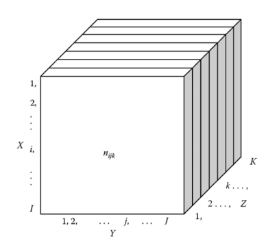
统计代写|属性数据分析作业代写analysis of categorical data代考|Modeling and the Generalized Linear Model
如果你也在 怎样代写属性数据分析analysis of categorical data这个学科遇到相关的难题,请随时右上角联系我们的24/7代写客服。
属性数据分析analysis of categorical data一属性变量和属性数据,通常所指属性数据,反映事物属性的数据,也称为定性数据或类别数据,它是属性变量取的值。分类数据是指将一个观察结果归入一个或多个类别的数据。例如,一个项目可能被评判为好或坏,或者对调查的反应可能包括同意、不同意或无意见等类别。Statgraphics包括许多处理这类数据的程序,包括包含在方差分析、回归分析和统计过程控制部分的建模程序。
statistics-lab™ 为您的留学生涯保驾护航 在代写属性数据分析analysis of categorical data方面已经树立了自己的口碑, 保证靠谱, 高质且原创的统计Statistics代写服务。我们的专家在代写属性数据分析analysis of categorical data方面经验极为丰富,各种代写属性数据分析analysis of categorical data相关的作业也就用不着说。
我们提供的属性数据分析analysis of categorical data及其相关学科的代写,服务范围广, 其中包括但不限于:
- Statistical Inference 统计推断
- Statistical Computing 统计计算
- Advanced Probability Theory 高等楖率论
- Advanced Mathematical Statistics 高等数理统计学
- (Generalized) Linear Models 广义线性模型
- Statistical Machine Learning 统计机器学习
- Longitudinal Data Analysis 纵向数据分析
- Foundations of Data Science 数据科学基础
统计代写|属性数据分析作业代写analysis of categorical data代考|The Random Component
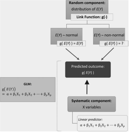
The random component of a GLM is the probability distribution assumed to underlie the dependent or outcome variable, predicted by the model. Recall from Chapter 2 that when we have continuous outcome variables, we typically assume that the values obtained for these variables are random observations that come from (or follow) a normal distribution. In other words, when the outcome or response variable is continuous, such as in simple linear regression or analysis of variance (ANOVA), we typically assume that the normal distribution is the random component or underlying probability distribution for the outcome variable.
When the outcome variable is categorical, we can no longer assume that its values in the population are normally distributed. In fact, in a GLM the random component can be any known probability distribution. As discussed in Chapter 2 , with categorical variables the Poisson or binomial is often the appropriate underlying distribution, and that distribution would indicate the random component when the outcome or response variable is categorical. For example, if the outcome variable is whether a student passed (rather than failed) a test, we would assume that the underlying probability distribution of the outcome is the binomial distribution rather than the normal distribution. As another example, if the outcome variable is the number of boats that dock at a particular marina in an hour, we would assume that the underlying probability distribution is the Poisson distribution rather than the normal distribution.
The random component of a GLM thus allows us to use outcome variables (Ys) that are not necessarily normally distributed. In addition, as was shown in Chapter 2 , the random component or distribution underlying the outcome variable $(Y)$ is instrumental in computing its expected value (or mean),
$$
E(Y)=\propto
$$
This expected value is also the outcome predicted by a model, using predictor variables.
统计代写|属性数据分析作业代写analysis of categorical data代考|The Systematic Component
The systematic component of a GLM consists of the independent, predictor, or explanatory variables (Xs) that a researcher hypothesizes will predict (or explain) differences in the dependent or outcome variable. The predictors are considered to be the systematic component of the model because they systematically explain differences in the outcome variable and are generally treated as fixed, rather than random, variables. These variables may be subject to experimental control, or systematic manipulation, although this is not a necessary condition for the systematic component.
The predictor variables are combined to form the linear predictor, which is simply a linear combination of the predictors or the “right-hand side” of the model equation.
where the coefficients of the model ( $\alpha$ and $\beta$ s) are estimated based on the observed data. The systematic component of a GLM thus specifies the way in which the explanatory variables or predictors are expected to linearly influence the predicted or expected value of the outcome, $E(Y)$.
It should be noted that each of the predictors may be a combination of other predictors. For example, an interaction term can be represented by a predictor that is the product of two variables, such as $X_{4}=X_{1} X_{3}$, or a nonlinear trend can be represented by a predictor that is a function of a variable, such as using $X_{2}=X_{1}^{2}$ to represent a quadratic trend by squaring a variable. The key is that the predictors are represented as a linear combination in the GLM to ensure that it is indeed a linear model.
统计代写|属性数据分析作业代写analysis of categorical data代考|The Link Function
The key to GLMs is to “link” the random and systematic components of the model with some mathematical function, which we will call $g(\cdot)$. This function is applied to the expected value of the outcome variable, $E(Y)$, so that it can be properly modeled or predicted using the systematic component; that is:
$$
\mathrm{g}(E(Y))=\alpha+\beta_{1} X_{1}+\beta_{2} X_{2}+\ldots+\beta_{p} X_{p}
$$
The link function allows us to relate the systematic component (consisting of a linear predictor) to the random component (which is based on the probability distribution of the outcome variable) in a linear manner. In other words, the link function is a mathematical function we use to transform the predicted or expected value of the outcome to produce a transformed variable, $\mathrm{g}(E(Y))$, that is linearly related to the predictors.
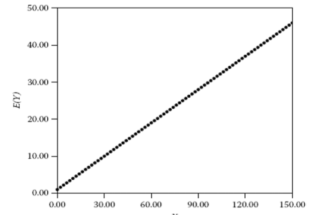
For example, suppose that we would like to use family income (in thousands of dollars) as a predictor, $X$, of a standardized test score (such as an ACT score). Figure $6.2$ provides an illustration of a possible relationship between these variables. In this case, if the relationship depicted in Figure $6.2$ provides a good representation of the actual relationship between these variables, the predicted outcome (ACT score), which is the expected value of $Y$ and is denoted as $E(Y)$, can be written as
$$
E(Y)=\alpha+\beta(X) . \mathrm{w}
$$
Figure $6.2$ shows that as $X$ increases by one unit, the predicted outcome, $E(Y)$, increases at a constant rate (represented by $\beta$ in Equation 6.1). In this case, the predicted or expected outcome, $E(Y)$, does not need to be transformed to be linearly related to the predictor. More technically, if $g(\cdot)$ represents the link function, the transformation of $E(Y)$ by $g$ in this case is$g(E(Y))=E(Y)$. This is referred to as the identity link function because applying the $g(\cdot)$ function to $E(Y)$ results in the same value, $E(Y)$. This would be a reasonable approach, in that it will represent the relationship appropriately, when the outcome variable is continuous. Thus, this is the link function that is used when the outcome or response variable is continuous and typically normally distributed, such as in regression and ANOVA models. In this case a link function is not truly necessary, though in the context of a GLM the link function would be the identity function.
When it cannot be assumed that the response variable follows a normal distribution, the predicted or expected outcome $E(Y)$ will not typically be linearly related to the predictors unless it is transformed. For example, suppose that the outcome variable was the probability that a student will pass (as opposed to fail) a specific test, so the predicted value is $E(Y)=\pi=$ predicted probability of passing. Using the same predictor as earlier $(X=$ family income), the graph shown in Figure 6.3a illustrates a possible relationship between these two variables. Note that in this case the outcome variable, a probability, cannot be lower than 0 or greater than 1 (by definition) no matter how high or low the value of the predictor gets. In addition, family income tends to be more strongly associated with the probability of passing the test for students in the middle of the family income range than at more extreme (very high or very low) income levels. In this case, using the identity link as in Equation $6.1$ to link the random and systematic components of the GLM would amount to using the model $E(Y)=\pi=\alpha+\beta(X)$ or fitting a straight line to the points in Figure 6.3a. This would result in a poor representation of the association between the variables, especially for certain income ranges. It would also then be theoretically possible for the prediction obtained from the model to exceed 1 or fall below 0 (for high or low enough values of $X$, respectively), which is nonsensical because probabilities must fall between 0 and 1 . If, however, the predicted probability $(E(Y)$ or $\pi)$ is transformed using the equation
$\mathrm{g}(E(Y))=\mathrm{g}(\pi)=\ln \left(\frac{\pi}{1-\pi}\right)=\operatorname{logit}$ of $\pi$,
then the resulting relationship between the transformed value, $\ln (\pi /(1-\pi))$, and income level $(\mathrm{X})$ will be linear, as illustrated in Figure 6.3b. Therefore, the transformed outcome variable can be related (or linked) to the predictor in a linear fashion by the following model:
$$
\mathrm{g}(E(Y))=\ln \left(\frac{\pi}{1-\pi}\right)=\alpha+\beta(X)
$$
This particular link function (or transformation) is called the logit link function, and the resulting GLM is called the logistic regression model (discussed in detail in Chapters 8,9 , and 10 ). The logit function typically works well with a binary outcome variable or a random component that is assumed to follow a binomial distribution.
属性数据分析
统计代写|属性数据分析作业代写analysis of categorical data代考|The Random Component
GLM 的随机分量是假设为模型预测的因变量或结果变量的概率分布。回想一下第 2 章,当我们有连续的结果变量时,我们通常假设为这些变量获得的值是来自(或遵循)正态分布的随机观察值。换句话说,当结果或响应变量是连续的时,例如在简单线性回归或方差分析 (ANOVA) 中,我们通常假设正态分布是结果变量的随机分量或潜在概率分布。
当结果变量是分类变量时,我们不能再假设它在总体中的值是正态分布的。事实上,在 GLM 中,随机分量可以是任何已知的概率分布。正如第 2 章所讨论的,对于分类变量,泊松或二项式通常是适当的基础分布,并且当结果或响应变量是分类变量时,该分布将指示随机分量。例如,如果结果变量是学生是否通过(而不是失败)测试,我们将假设结果的潜在概率分布是二项分布而不是正态分布。再举一个例子,如果结果变量是一小时内停靠在特定码头的船只数量,
因此,GLM 的随机分量允许我们使用不一定是正态分布的结果变量 (Ys)。此外,如第 2 章所示,结果变量的随机分量或分布(是)有助于计算其预期值(或平均值),
和(是)=∝
该预期值也是模型使用预测变量预测的结果。
统计代写|属性数据分析作业代写analysis of categorical data代考|The Systematic Component
GLM 的系统组件由独立变量、预测变量或解释变量 (X) 组成,研究人员假设这些变量将预测(或解释)因变量或结果变量的差异。预测变量被认为是模型的系统组成部分,因为它们系统地解释了结果变量的差异,并且通常被视为固定变量,而不是随机变量。这些变量可能受到实验控制或系统操作,尽管这不是系统组件的必要条件。
预测变量组合起来形成线性预测变量,它只是预测变量的线性组合或模型方程的“右手边”。
其中模型的系数 (一种和bs) 根据观察到的数据进行估计。因此,GLM 的系统组件指定了解释变量或预测变量预期线性影响结果的预测值或预期值的方式,和(是).
应当注意,每个预测器可以是其他预测器的组合。例如,一个交互项可以由一个预测变量表示,该预测变量是两个变量的乘积,例如X4=X1X3, 或者非线性趋势可以用作为变量函数的预测变量来表示,例如使用X2=X12通过对变量进行平方来表示二次趋势。关键是预测变量在 GLM 中表示为线性组合,以确保它确实是一个线性模型。
统计代写|属性数据分析作业代写analysis of categorical data代考|The Link Function
GLM 的关键是将模型的随机和系统组件与一些数学函数“联系起来”,我们将其称为G(⋅). 该函数应用于结果变量的期望值,和(是),以便可以使用系统组件对其进行适当的建模或预测;那是:
G(和(是))=一种+b1X1+b2X2+…+bpXp
链接函数允许我们以线性方式将系统分量(由线性预测变量组成)与随机分量(基于结果变量的概率分布)联系起来。换句话说,链接函数是我们用来转换结果的预测值或期望值以产生转换变量的数学函数,G(和(是)),即与预测变量线性相关。
例如,假设我们想使用家庭收入(以千美元计)作为预测变量,X,标准化考试成绩(如 ACT 成绩)。数字6.2说明了这些变量之间可能存在的关系。在这种情况下,如果如图所示的关系6.2提供了这些变量之间实际关系的良好表示,即预测结果(ACT 分数),即是并表示为和(是), 可以写成
和(是)=一种+b(X).在
数字6.2表明作为X增加一个单位,预测结果,和(是),以恒定速率增加(表示为b在公式 6.1)。在这种情况下,预测或预期的结果,和(是), 不需要转换为与预测变量线性相关。从技术上讲,如果G(⋅)表示链接函数,变换和(是)经过G在这种情况下是G(和(是))=和(是). 这被称为身份链接功能,因为应用G(⋅)作用于和(是)产生相同的值,和(是). 这将是一种合理的方法,因为当结果变量是连续的时,它将适当地表示关系。因此,这是当结果或响应变量是连续的并且通常是正态分布时使用的链接函数,例如在回归和方差分析模型中。在这种情况下,链接函数并不是真正需要的,尽管在 GLM 的上下文中,链接函数将是恒等函数。
当不能假设响应变量服从正态分布时,预测或预期结果和(是)除非它被转换,否则它通常不会与预测变量线性相关。例如,假设结果变量是学生通过(而不是不及格)特定测试的概率,因此预测值为和(是)=圆周率=预测的通过概率。使用与之前相同的预测器(X=家庭收入),图 6.3a 中的图表说明了这两个变量之间可能存在的关系。请注意,在这种情况下,无论预测变量的值有多高或多低,结果变量(概率)都不能小于 0 或大于 1(根据定义)。此外,与极端(非常高或非常低)收入水平的学生相比,家庭收入中等的学生与通过考试的概率之间的联系更紧密。在这种情况下,使用等式中的身份链接6.1将 GLM 的随机和系统成分联系起来相当于使用该模型和(是)=圆周率=一种+b(X)或将直线拟合到图 6.3a 中的点。这将导致变量之间的关联表现不佳,特别是对于某些收入范围。从理论上讲,从模型获得的预测也有可能超过 1 或低于 0(对于足够高或足够低的X,分别),这是无意义的,因为概率必须落在 0 和 1 之间。但是,如果预测的概率(和(是)或者圆周率)使用等式转换
G(和(是))=G(圆周率)=ln(圆周率1−圆周率)=罗吉特的圆周率,
然后是转换后的值之间的关系,ln(圆周率/(1−圆周率)), 和收入水平(X)将是线性的,如图 6.3b 所示。因此,转换后的结果变量可以通过以下模型以线性方式与预测变量相关(或链接):
G(和(是))=ln(圆周率1−圆周率)=一种+b(X)
这个特定的链接函数(或转换)称为 logit 链接函数,生成的 GLM 称为逻辑回归模型(在第 8,9 和 10 章中详细讨论)。logit 函数通常适用于二元结果变量或假定遵循二项分布的随机分量。

统计代写请认准statistics-lab™. statistics-lab™为您的留学生涯保驾护航。统计代写|python代写代考
随机过程代考
在概率论概念中,随机过程是随机变量的集合。 若一随机系统的样本点是随机函数,则称此函数为样本函数,这一随机系统全部样本函数的集合是一个随机过程。 实际应用中,样本函数的一般定义在时间域或者空间域。 随机过程的实例如股票和汇率的波动、语音信号、视频信号、体温的变化,随机运动如布朗运动、随机徘徊等等。
贝叶斯方法代考
贝叶斯统计概念及数据分析表示使用概率陈述回答有关未知参数的研究问题以及统计范式。后验分布包括关于参数的先验分布,和基于观测数据提供关于参数的信息似然模型。根据选择的先验分布和似然模型,后验分布可以解析或近似,例如,马尔科夫链蒙特卡罗 (MCMC) 方法之一。贝叶斯统计概念及数据分析使用后验分布来形成模型参数的各种摘要,包括点估计,如后验平均值、中位数、百分位数和称为可信区间的区间估计。此外,所有关于模型参数的统计检验都可以表示为基于估计后验分布的概率报表。
广义线性模型代考
广义线性模型(GLM)归属统计学领域,是一种应用灵活的线性回归模型。该模型允许因变量的偏差分布有除了正态分布之外的其它分布。
statistics-lab作为专业的留学生服务机构,多年来已为美国、英国、加拿大、澳洲等留学热门地的学生提供专业的学术服务,包括但不限于Essay代写,Assignment代写,Dissertation代写,Report代写,小组作业代写,Proposal代写,Paper代写,Presentation代写,计算机作业代写,论文修改和润色,网课代做,exam代考等等。写作范围涵盖高中,本科,研究生等海外留学全阶段,辐射金融,经济学,会计学,审计学,管理学等全球99%专业科目。写作团队既有专业英语母语作者,也有海外名校硕博留学生,每位写作老师都拥有过硬的语言能力,专业的学科背景和学术写作经验。我们承诺100%原创,100%专业,100%准时,100%满意。
机器学习代写
随着AI的大潮到来,Machine Learning逐渐成为一个新的学习热点。同时与传统CS相比,Machine Learning在其他领域也有着广泛的应用,因此这门学科成为不仅折磨CS专业同学的“小恶魔”,也是折磨生物、化学、统计等其他学科留学生的“大魔王”。学习Machine learning的一大绊脚石在于使用语言众多,跨学科范围广,所以学习起来尤其困难。但是不管你在学习Machine Learning时遇到任何难题,StudyGate专业导师团队都能为你轻松解决。
多元统计分析代考
基础数据: $N$ 个样本, $P$ 个变量数的单样本,组成的横列的数据表
变量定性: 分类和顺序;变量定量:数值
数学公式的角度分为: 因变量与自变量
时间序列分析代写
随机过程,是依赖于参数的一组随机变量的全体,参数通常是时间。 随机变量是随机现象的数量表现,其时间序列是一组按照时间发生先后顺序进行排列的数据点序列。通常一组时间序列的时间间隔为一恒定值(如1秒,5分钟,12小时,7天,1年),因此时间序列可以作为离散时间数据进行分析处理。研究时间序列数据的意义在于现实中,往往需要研究某个事物其随时间发展变化的规律。这就需要通过研究该事物过去发展的历史记录,以得到其自身发展的规律。
回归分析代写
多元回归分析渐进(Multiple Regression Analysis Asymptotics)属于计量经济学领域,主要是一种数学上的统计分析方法,可以分析复杂情况下各影响因素的数学关系,在自然科学、社会和经济学等多个领域内应用广泛。
MATLAB代写
MATLAB 是一种用于技术计算的高性能语言。它将计算、可视化和编程集成在一个易于使用的环境中,其中问题和解决方案以熟悉的数学符号表示。典型用途包括:数学和计算算法开发建模、仿真和原型制作数据分析、探索和可视化科学和工程图形应用程序开发,包括图形用户界面构建MATLAB 是一个交互式系统,其基本数据元素是一个不需要维度的数组。这使您可以解决许多技术计算问题,尤其是那些具有矩阵和向量公式的问题,而只需用 C 或 Fortran 等标量非交互式语言编写程序所需的时间的一小部分。MATLAB 名称代表矩阵实验室。MATLAB 最初的编写目的是提供对由 LINPACK 和 EISPACK 项目开发的矩阵软件的轻松访问,这两个项目共同代表了矩阵计算软件的最新技术。MATLAB 经过多年的发展,得到了许多用户的投入。在大学环境中,它是数学、工程和科学入门和高级课程的标准教学工具。在工业领域,MATLAB 是高效研究、开发和分析的首选工具。MATLAB 具有一系列称为工具箱的特定于应用程序的解决方案。对于大多数 MATLAB 用户来说非常重要,工具箱允许您学习和应用专业技术。工具箱是 MATLAB 函数(M 文件)的综合集合,可扩展 MATLAB 环境以解决特定类别的问题。可用工具箱的领域包括信号处理、控制系统、神经网络、模糊逻辑、小波、仿真等。

![PDF] Binary models for marginal independence | Semantic Scholar](data:image/svg+xml,%3Csvg%20xmlns='http://www.w3.org/2000/svg'%20viewBox='0%200%20545%20131'%3E%3C/svg%3E)