如果你也在 怎样代写属性数据分析analysis of categorical data这个学科遇到相关的难题,请随时右上角联系我们的24/7代写客服。
属性数据分析analysis of categorical data一属性变量和属性数据,通常所指属性数据,反映事物属性的数据,也称为定性数据或类别数据,它是属性变量取的值。分类数据是指将一个观察结果归入一个或多个类别的数据。例如,一个项目可能被评判为好或坏,或者对调查的反应可能包括同意、不同意或无意见等类别。Statgraphics包括许多处理这类数据的程序,包括包含在方差分析、回归分析和统计过程控制部分的建模程序。
statistics-lab™ 为您的留学生涯保驾护航 在代写属性数据分析analysis of categorical data方面已经树立了自己的口碑, 保证靠谱, 高质且原创的统计Statistics代写服务。我们的专家在代写属性数据分析analysis of categorical data方面经验极为丰富,各种代写属性数据分析analysis of categorical data相关的作业也就用不着说。
我们提供的属性数据分析analysis of categorical data及其相关学科的代写,服务范围广, 其中包括但不限于:
- Statistical Inference 统计推断
- Statistical Computing 统计计算
- Advanced Probability Theory 高等楖率论
- Advanced Mathematical Statistics 高等数理统计学
- (Generalized) Linear Models 广义线性模型
- Statistical Machine Learning 统计机器学习
- Longitudinal Data Analysis 纵向数据分析
- Foundations of Data Science 数据科学基础

统计代写|属性数据分析作业代写analysis of categorical data代考|Partial Tables and Conditional Associations
Three-way contingency tables depict the relationship between three categorical variables by considering two-way contingency tables, called partial tables, at the different levels of
Associations, Three Categorical Variables 87 the third variable. While the notation and terminology introduced in the previous chapter for two-way contingency tables generalize to three-way contingency tables, they are here extended to take into consideration the third variable.
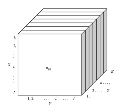
When we have three categorical variables, the total number of categories for the row variable, $X$, is still denoted by $I$, with each category indexed by $i$; the total number of categories for the column variable, $Y$, is still denoted by $J$, with each category indexed by $j$; but now we have a third variable, $Z$, for which the total number of categories is denoted by $K$, with each category indexed by $k$. Figure $5.1$ illustrates a three-way table, which can be partitioned or “sliced up” in three different ways to create partial tables. One could either create $K$ partial tables, one for each level of the variable $Z$; J partial tables, one for each level of $Y$; or $I$ partial tables, one for each level of $X$. The slices for each level of $Z$ are depicted in Figure 5.1. The “slices” are often displayed side-by-side or stacked on top of each other when presenting the data. In general, the size of three-way contingency tables is denoted as $I \times J \times K$ and the frequency in each cell of the table (i.e., the number of observations falling into the $i^{\text {th }}$ category of $X, j^{\text {th }}$ category of $Y$, and $k^{\text {th }}$ category of $Z$ ) is denoted by $n_{i j k}$.
A substantive example of a three-way contingency table depicting the relationship between political affiliation, age, and gender is illustrated in Table 5.1. In this example, $X$ is political affiliation and has $I=3$ categories ( $i=1$ for liberal; $i=2$ for moderate; and $i=3$ for conservative), $Y$ is age group and has $J=4$ categories $(j=1$ for those $18-29$ years of age; $j=2$ for those $30-39$ years of age; $j=3$ for those $40-49$ years of age; and $j=4$ for those $50-$ plus years of age), and $Z$ is gender with $K=2$ categories ( $k=1$ for males; $k=2$ for females). The size of this three-way contingency table is $3 \times 4 \times 2$. The frequency in each cell of the table is denoted by $\mathrm{n}{\mathrm{ijl}}$ (where $i=1,2, \ldots, 3 ; j=1,2, \ldots, 4 ; k=1,2$ ). For example, $\mathrm{n}{142}$ in Table $5.1$ represents the number of respondents who are liberal $(i=1), 50$-plus years of age $(j=4)$, and female $(k=2)$, so $n_{142}=63$. Taken together, the cell frequencies represent the joint distribution of the three categorical variables.
统计代写|属性数据分析作业代写analysis of categorical data代考|Marginal Tables and Marginal Associations
A marginal table represents combined partial tables and is formed by adding their corresponding frequencies. That is, the marginal table contains marginal frequencies because the frequencies are summed across one of the three variables. Using the example in Table 5.1, a $3 \times 4$ marginal table (representing political affiliation and age category) can be formed by adding the frequencies across gender, as depicted in Table 5.3. For illustration, the first cell frequency in Table $5.3$ is $\mathrm{n}{11+}=86$ and was obtained by adding the frequencies of males and females who are liberal and $18-29$ years old; that is, $n{111}+n_{112}=27+59=86$. In general, each frequency in this marginal table can be represented as $n_{i j+}=n_{i j 1}+n_{i j 2}$.
The associations in marginal tables are called marginal associations. For readers familiar with analysis of variance (ANOVA), the conditional associations previously discussed are analogous to three-way interactions in ANOVA, where the interaction between any two factors depends on the level of the third factor, while the marginal associations are analogous to
two-way interactions in a three-way ANOVA, where the interaction between any two factors is averaged across all levels of the third factor. In other words, conditional associations examine two-way associations separately at each level of the third variable, whereas marginal associations examine two-way associations overall, essentially ignoring the third variable. Therefore, conditional associations can be very different from the marginal associations for the same data set. In our example, the marginal association between political affiliation and age group would essentially ignore one’s gender and may be very different from either of the conditional associations for these variables (which are obtained for each gender separately).
To further illustrate these concepts, Table $5.4$ depicts the results of a study, adapted from Agresti (1990), that examined the association between smoking status and the ability to breathe normally for two age groups. A marginal table that depicts the overall association between smoking status and the ability to breathe normally regardless of (or summed across) age is shown in Table 5.5. The estimated odds ratio for the marginal association between breathing normally and smoking status (computed using the frequencies in Table 5.5) is
$$
\hat{\theta}=\frac{741 \times 131}{927 \times 38}=2.756
$$
Associations, Three Categorical Variables 91 and it represents a statistically significant marginal association $\left(\chi^{2}=30.242, d f=1, p<0.001\right)$. In computing this association, we have ignored the effect of age, although it might be hypothesized to have an impact on the ability to breathe. In fact, using the partial tables shown in Table $5.4$, for those who were less than 50 years of age, the estimated odds ratio between breathing normally and smoking status is $\hat{\theta}=1.418$, which is not a statistically significant conditional association $\left(\chi^{2}=2.456, d f=1, p=0.112\right)$. On the other hand, for participants in the study who were 50 years of age or older, the estimated odds ratio is $\hat{\theta}=12.38$, which is a statistically significant conditional association $\left(\chi^{2}=35.45, d f=1, p<0.001\right)$. Therefore, age is an important covariate in studying the relationship between smoking status and the ability to breathe.
统计代写|属性数据分析作业代写analysis of categorical data代考|Patterns of Association
In this section, we discuss the relationship between two variables, $X$ and $Y$, either conditional on or combined across the levels of the third variable, $Z$. Although the labels given to the variables (i.e., which variable is called $X, Y$, or $Z$ ) are rather arbitrary, it is somewhat conventional to denote the primary variables of interest as $X$ and $Y$ while denoting the covariate as $Z$. This is the approach we take in the general discussion that follows.
属性数据分析
统计代写|属性数据分析作业代写analysis of categorical data代考|Partial Tables and Conditional Associations
三向列联表通过考虑双向列联表(称为部分表)来描述三个分类变量之间的关系,在不同的
关联级别,三分类变量 87 第三个变量。虽然前一章介绍的双向列联表的符号和术语可以推广到三路列联表,但在这里它们被扩展以考虑第三个变量。
当我们有三个分类变量时,行变量的类别总数,X, 仍表示为一世,每个类别由一世; 列变量的类别总数,是, 仍表示为Ĵ,每个类别由j; 但现在我们有了第三个变量,从, 其中类别总数表示为到,每个类别由到. 数字5.1说明了一个三向表,可以以三种不同的方式对其进行分区或“切片”以创建部分表。一个人可以创建到部分表,一个用于变量的每个级别从; J 个部分表,每个级别一个是; 或者一世部分表,每个级别一个X. 每个级别的切片从如图 5.1 所示。在呈现数据时,“切片”通常并排显示或堆叠在一起。通常,三向列联表的大小表示为一世×Ĵ×到以及表格每个单元格中的频率(即,落入一世th 类别X,jth 类别是, 和到th 类别从) 表示为n一世j到.
描述政治派别、年龄和性别之间关系的三向列联表的一个实质性例子如表 5.1 所示。在这个例子中,X是政治派别,并且有一世=3类别(一世=1对于自由主义者;一世=2为中度;和一世=3保守),是是年龄组并且有Ĵ=4类别(j=1对于那些18−29岁;j=2对于那些30−39岁;j=3对于那些40−49岁; 和j=4对于那些50−加上年龄),和从是性别与到=2类别(到=1男性;到=2对于女性)。这个三向列联表的大小是3×4×2. 表中每个单元格中的频率用 $\mathrm{n} {\mathrm{ijl}} 表示(在H和r和i=1,2, \ldots, 3 ; j=1,2, \ldots, 4 ; k=1,2).F这r和X一种米p一世和,\mathrm{n} {142}一世n吨一种b一世和5.1r和pr和s和n吨s吨H和n你米b和r这Fr和sp这nd和n吨s在H这一种r和一世一世b和r一种一世(i=1), 50−p一世你s是和一种rs这F一种G和(j=4),一种ndF和米一种一世和(k = 2),s这n_{142}=63 美元。总之,单元频率代表三个分类变量的联合分布。
统计代写|属性数据分析作业代写analysis of categorical data代考|Marginal Tables and Marginal Associations
边缘表表示组合的部分表,并通过添加它们的相应频率形成。也就是说,边际表包含边际频率,因为频率是三个变量之一的总和。使用表 5.1 中的示例,a3×4边际表(代表政治派别和年龄类别)可以通过添加跨性别的频率来形成,如表 5.3 所示。为了说明,表中的第一个小区频率5.3是 $\mathrm{n} {11+}=86一种nd在一种s这b吨一种一世n和db是一种dd一世nG吨H和Fr和q你和nC一世和s这F米一种一世和s一种ndF和米一种一世和s在H这一种r和一世一世b和r一种一世一种nd18-29是和一种rs这一世d;吨H一种吨一世s,n {111}+n_{112}=27+59=86.一世nG和n和r一种一世,和一种CHFr和q你和nC是一世n吨H一世s米一种rG一世n一种一世吨一种b一世和C一种nb和r和pr和s和n吨和d一种sn_{i j+}=n_{ij 1}+n_{ij 2}$。
边缘表中的关联称为边缘关联。对于熟悉方差分析 (ANOVA) 的读者来说,前面讨论的条件关联类似于 ANOVA 中的三向交互作用,其中任意两个因素之间的交互作用取决于第三个因素的水平,而边际关联类似于
三向方差分析中的双向交互作用,其中任何两个因素之间的交互作用在第三个因素的所有水平上取平均值。换句话说,条件关联在第三个变量的每个级别分别检查双向关联,而边际关联总体上检查双向关联,基本上忽略了第三个变量。因此,条件关联可能与同一数据集的边缘关联非常不同。在我们的示例中,政治派别和年龄组之间的边际关联基本上会忽略一个人的性别,并且可能与这些变量的任何一个条件关联(分别针对每个性别获得)非常不同。
为了进一步说明这些概念,表5.4描述了改编自 Agresti (1990) 的一项研究的结果,该研究检查了两个年龄组的吸烟状况与正常呼吸能力之间的关系。表 5.5 显示了一个边际表,该表描述了吸烟状况与正常呼吸能力之间的总体关联,而与年龄无关(或总和)。正常呼吸与吸烟状态之间的边际关联的估计优势比(使用表 5.5 中的频率计算)为
θ^=741×131927×38=2.756
关联,三个分类变量 91 它代表了具有统计意义的边际关联(χ2=30.242,dF=1,p<0.001). 在计算这种关联时,我们忽略了年龄的影响,尽管可能假设它对呼吸能力有影响。实际上,使用 Table 所示的部分表5.4,对于年龄小于 50 岁的人,正常呼吸和吸烟状态之间的估计优势比为θ^=1.418,这不是统计显着的条件关联(χ2=2.456,dF=1,p=0.112). 另一方面,对于年龄在 50 岁或以上的研究参与者,估计优势比为θ^=12.38,这是一个统计显着的条件关联(χ2=35.45,dF=1,p<0.001). 因此,年龄是研究吸烟状况与呼吸能力之间关系的重要协变量。
统计代写|属性数据分析作业代写analysis of categorical data代考|Patterns of Association
在本节中,我们讨论两个变量之间的关系,X和是,以第三个变量的水平为条件或组合,从. 虽然赋予变量的标签(即调用哪个变量X,是, 或者从) 是相当随意的,将感兴趣的主要变量表示为有些传统X和是同时将协变量表示为从. 这是我们在随后的一般性讨论中采用的方法。

统计代写请认准statistics-lab™. statistics-lab™为您的留学生涯保驾护航。统计代写|python代写代考
随机过程代考
在概率论概念中,随机过程是随机变量的集合。 若一随机系统的样本点是随机函数,则称此函数为样本函数,这一随机系统全部样本函数的集合是一个随机过程。 实际应用中,样本函数的一般定义在时间域或者空间域。 随机过程的实例如股票和汇率的波动、语音信号、视频信号、体温的变化,随机运动如布朗运动、随机徘徊等等。
贝叶斯方法代考
贝叶斯统计概念及数据分析表示使用概率陈述回答有关未知参数的研究问题以及统计范式。后验分布包括关于参数的先验分布,和基于观测数据提供关于参数的信息似然模型。根据选择的先验分布和似然模型,后验分布可以解析或近似,例如,马尔科夫链蒙特卡罗 (MCMC) 方法之一。贝叶斯统计概念及数据分析使用后验分布来形成模型参数的各种摘要,包括点估计,如后验平均值、中位数、百分位数和称为可信区间的区间估计。此外,所有关于模型参数的统计检验都可以表示为基于估计后验分布的概率报表。
广义线性模型代考
广义线性模型(GLM)归属统计学领域,是一种应用灵活的线性回归模型。该模型允许因变量的偏差分布有除了正态分布之外的其它分布。
statistics-lab作为专业的留学生服务机构,多年来已为美国、英国、加拿大、澳洲等留学热门地的学生提供专业的学术服务,包括但不限于Essay代写,Assignment代写,Dissertation代写,Report代写,小组作业代写,Proposal代写,Paper代写,Presentation代写,计算机作业代写,论文修改和润色,网课代做,exam代考等等。写作范围涵盖高中,本科,研究生等海外留学全阶段,辐射金融,经济学,会计学,审计学,管理学等全球99%专业科目。写作团队既有专业英语母语作者,也有海外名校硕博留学生,每位写作老师都拥有过硬的语言能力,专业的学科背景和学术写作经验。我们承诺100%原创,100%专业,100%准时,100%满意。
机器学习代写
随着AI的大潮到来,Machine Learning逐渐成为一个新的学习热点。同时与传统CS相比,Machine Learning在其他领域也有着广泛的应用,因此这门学科成为不仅折磨CS专业同学的“小恶魔”,也是折磨生物、化学、统计等其他学科留学生的“大魔王”。学习Machine learning的一大绊脚石在于使用语言众多,跨学科范围广,所以学习起来尤其困难。但是不管你在学习Machine Learning时遇到任何难题,StudyGate专业导师团队都能为你轻松解决。
多元统计分析代考
基础数据: $N$ 个样本, $P$ 个变量数的单样本,组成的横列的数据表
变量定性: 分类和顺序;变量定量:数值
数学公式的角度分为: 因变量与自变量
时间序列分析代写
随机过程,是依赖于参数的一组随机变量的全体,参数通常是时间。 随机变量是随机现象的数量表现,其时间序列是一组按照时间发生先后顺序进行排列的数据点序列。通常一组时间序列的时间间隔为一恒定值(如1秒,5分钟,12小时,7天,1年),因此时间序列可以作为离散时间数据进行分析处理。研究时间序列数据的意义在于现实中,往往需要研究某个事物其随时间发展变化的规律。这就需要通过研究该事物过去发展的历史记录,以得到其自身发展的规律。
回归分析代写
多元回归分析渐进(Multiple Regression Analysis Asymptotics)属于计量经济学领域,主要是一种数学上的统计分析方法,可以分析复杂情况下各影响因素的数学关系,在自然科学、社会和经济学等多个领域内应用广泛。
MATLAB代写
MATLAB 是一种用于技术计算的高性能语言。它将计算、可视化和编程集成在一个易于使用的环境中,其中问题和解决方案以熟悉的数学符号表示。典型用途包括:数学和计算算法开发建模、仿真和原型制作数据分析、探索和可视化科学和工程图形应用程序开发,包括图形用户界面构建MATLAB 是一个交互式系统,其基本数据元素是一个不需要维度的数组。这使您可以解决许多技术计算问题,尤其是那些具有矩阵和向量公式的问题,而只需用 C 或 Fortran 等标量非交互式语言编写程序所需的时间的一小部分。MATLAB 名称代表矩阵实验室。MATLAB 最初的编写目的是提供对由 LINPACK 和 EISPACK 项目开发的矩阵软件的轻松访问,这两个项目共同代表了矩阵计算软件的最新技术。MATLAB 经过多年的发展,得到了许多用户的投入。在大学环境中,它是数学、工程和科学入门和高级课程的标准教学工具。在工业领域,MATLAB 是高效研究、开发和分析的首选工具。MATLAB 具有一系列称为工具箱的特定于应用程序的解决方案。对于大多数 MATLAB 用户来说非常重要,工具箱允许您学习和应用专业技术。工具箱是 MATLAB 函数(M 文件)的综合集合,可扩展 MATLAB 环境以解决特定类别的问题。可用工具箱的领域包括信号处理、控制系统、神经网络、模糊逻辑、小波、仿真等。