In computing time and space complexities, we want to ignore constant factors and performance on small inputs, because we know that constant factors depend strongly on features of our model that we usually don’t care much about, and performance on small inputs can always be faked by baking a large lookup table into our finite-state controller. As in the usual analysis of algorithms, we get around these issues by expressing performance using asymptotic notation. This section gives a brief review of asymptotic notation as used in algorithm analysis and computational complexity theory. Given two non-negative ${ }^4$ functions $f(n)$ and $g(n)$, we say that:
$f(n)=O(g(n))$ if there exist constants $c>0$ and $N$ such that $f(n) \leq$ $c \cdot g(n)$ for all $n \geq N$.
$f(n)=\Omega(g(n))$ if there exist constants $c>0$ and $N$ such that $f(n) \geq$ $c \cdot(g n)$ for all $n \geq N$.
$f(n)=\Theta(g(n))$ if $f(n)=O(g(n))$ and $f(n)=\Omega(g(n))$, or equivalently if there exist constants $c_1>0, c_2>0$, and $N$ such that $c_1 \cdot g(n) \leq$ $f(n) \leq c_2 \cdot g(n)$ for all $n \geq N$.
$f(n)=o(g(n))$ if for any constant $c>0$, there exists a constant $N$ such that $f(n) \leq c \cdot g(n)$ for all $n \geq N$.
$f(n)=\omega(g(n))$ if for any constant $c>0$, there exists a constant $N$ such that $f(n) \geq c \cdot g(n)$ for all $n \geq N$.
Note that we are using the equals sign in a funny way here. The convention is that given an asymptotic expression like $O(n)+O\left(n^2\right)=O\left(n^3\right)$, the statement is true if for all functions we could substitute in on the lefthand side in each class, there exist functions we could substitute in on the right-hand side to make it true. ${ }^5$
计算机代写|计算复杂度理论代写Computational complexity theory代考|Programming a Turing machine
Although one can in principle describe a Turing machine program by giving an explicit representation of $\delta$, no sane programmer would ever want to do this. I personally find it helpful to think about TM programming as if I were programming in a C-like language, where the tapes correspond to (infinite) arrays of characters and the head positions correspond to (highlyrestricted) pointers. The restrictions on the pointers are that we can’t do any pointer operations other than post-increment, post-decrement, dereference,
Table 3.1: Turing-machine transition function for reversing the input. In lines where $x$ appears in the input tape, it is assumed that $x$ is not zero. Note this is an abbreviated description: the actual transition function would not use variables $x$ and $y$ but would instead expand out all $|\Sigma|$ possible values for each. and assignment through a dereference; these correspond to moving the head left, moving the head right, reading a tape cell, and writing a tape cell. The state of the controller represents several aspects of the program. At minimum, the state encodes the current program counter (so this approach only works for code that doesn’t require a stack, which rules out recursion and many uses of subroutines). The state can also be used to hold a finite number of variables that can take on a finite number of values.
A computation of a predicate by a Turing machine proceeds as follows:
We start the machine in a standard initial configuration where the first tape contains the input. For convenience we typically assume that this is bounded by blank characters that cannot appear in the input. The head on the first tape starts on the leftmost input symbol. All cells on all tapes other than the input tape start off with a blank symbol, and the heads start in a predictable position. For the output tape, the head starts at the leftmost cell for writing the output. The controller starts in the initial state $q_0$.
Each step of the computation consists of reading the $k$-tuple of symbols under the $k$ heads, then rewriting these symbols, updating the state, and moving the heads, all according to the transition function.
This continues until the machine halts, which we defined above as reaching a configuration that doesn’t change as a result of applying the transition function.
The time complexity of an execution is the number of steps until the machine halts. Typically we will try to bound the time complexity as a function of the size $n$ of the input, defined as the number of cells occupied by the input, excluding the infinite number of blanks that surround it. The space complexity is the number of tape cells used by the computation. We have to be a little careful to define what it means to use a cell. A naive approach is just to count the number of cells that hold a non-blank symbol at any step of the computation, but this allows cheating (on a multi-tape Turing machine) because we can simulate an unbounded counter by writing a single non-blank symbol to one of our work tapes and using the position of the head relative to this symbol as the counter value. ${ }^3$
So instead we will charge for any cell that a head ever occupies, whether it writes a non-blank symbol to that cell or not.
An exception is that if we have a read-only input tape and a write-only output tape, we will only charge for cells on the work tapes. This allows space complexity sublinear in $n$.
计算机代写|计算复杂度理论代写Computational complexity theory代考|Problems and languages
For the most part, the kind of problems we study in complexity theory are decision problems, where we are presented with an input $x$ and have to answer “yes” or “no” based on whether $x$ satisfies some predicate $P$. An example is GRAPH 3-COLORABILITY: ${ }^1$ Given a graph $G$, is there a way to assign three colors to the vertices so that no edge has two endpoint of the same color?
Most of the algorithms you’ve probably seen have computed actual functions instead of just solving a decision problem, so the choice to limit ourselves (mostly) to decision problems requires some justification. The main reason is that decision problems are simpler to reason about than more general functions, and our life as complexity theorists is hard enough already. But we can also make some plausible excuses that decision problems in fact capture most of what is hard about function computation.
For example, if we are in the graph-coloring business, we probably want to find a coloring of $G$ rather than just be told that it exists. But if we have a machine that tells use whether or not a coloring exists, with a little tinkering we can turn it into a machine that tells us if a coloring exists consistent with locking down a few nodes to have particular colors. ${ }^2$ With this modified machine, we can probe potential colorings one vertex at a time, backing off if we place a color that prevents us from coloring the entire graph. Since we have to call the graph-coloring tester more than once, this is more expensive than the original decision problem, but it will still be reasonably cfficient if our algorithm for the decision problem is. Concentrating on decision problems fixes the outputs of what we are doing. We also have to formalize how we are handling inputs. Typically we assume that an instance $x$ of whatever problem we are looking at has an encoding $\llcorner x\lrcorner$ over some alphabet $\Sigma$, which can in principle always be reduced to just ${0,1}$. Under this assumption, the input tape contains a sequence of symbols from $\Sigma$ bounded by an infinite sequence of blanks in both directions. The input tape head by convention starts on the leftmost symbol in the input.
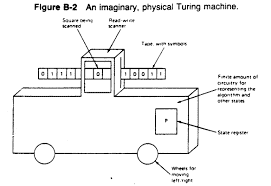
A Turing machine (TM for short) consists of one or more tapes, which we can think of as storing an infinite (in both directions) array of symbols from some alphabet $\Gamma$, one or more heads, which point to particular locations on the tape(s), and a finite-state control that controls the movement of the heads on the tapes and that may direct each head to rewrite the symbol in the cell it currently points to, based on the current symbols under the heads and its state, an element of its state space $Q$.
In its simplest form, a Turing machine has exactly one tape that is used for input, computation, and output, and has only one head on this tape. This is often too restrictive to program easily, so we will typically assume at least three tapes (with corresponding heads): one each for input, work, and output. This does not add any significant power to the model, and indeed not only is it possible for a one-tape Turing machine to simulate a $k$-tape Turing machine for any fixed $k$, it can do so with only polynomial slowdown. Similarly, even though in principle we can limit our alphabet to just ${0,1}$, we will in general assume whatever (finite) alphabet is convenient for the tape cells.
Formally, we can define a $k$-tape Turing machine as a tuple $\langle\Gamma, Q, \delta\rangle$, where $\Gamma$ is the alphabet; $Q$ is the state space of the finite-state controller, $q_0$ is the initial state; and $\delta: Q \times \Gamma^k \rightarrow Q \times \Gamma^k \times{\mathrm{L}, \mathrm{S}, \mathrm{R}}^k$ is the transition function, which specifies for each state $q \in Q$ and $k$-tuple of symbols from $\Gamma$ seen at the current positions of the heads the next state $q^{\prime} \in Q$, a new tuple of symbols to write to the current head positions, and a direction Left, Stay, or Right to move each head in. ${ }^2$
Some definitions of a Turing machine add additional details to the tuple, including an explicit blank symbol $b \in \Gamma$, a restricted input alphabet $\Sigma \subseteq \Gamma$ (which generally does not include $b$, since the blank regions of the input tape mark the ends of the input), an explicit starting state $q_0 \in Q$, and an explicit list of accepting states $A \subseteq Q$. We will include these details as needed. To avoid confusion between the state $q$ of the controller and the state of the Turing machine as a whole (which includes the contents of the tapes and the positions of the heads as well), we will describe the state of the machine as a whole as its configuration and reserve state for just the part of the configuration that represents the state of the controller.
In this section, we provide some tools to prove the elusiveness of a Boolean function. We begin with a simple one.
Theorem 5.10 A Boolean function with an odd number of truth assignments is elusive.
Proof. The constant functions $f \equiv 0$ and $f \equiv 1$ have 0 and $2^{n}$ truth assignments, respectively. Hence, a Boolean function with an odd number of truth assignments must be a nonconstant function. If $f$ has at least two variables and $x_{i}$ is one of them, then the number of truth assignments of $f$ is the sum of those of $\left.f\right|{x{i}=0}$ and $\left.f\right|{x{i}=1}$. Therefore, either $\left.f\right|{x{i}=0}$ or $\left.f\right|{x{i}=1}$ has an odd number of truth assignments and is not a constant function. Thus, for any decision tree computing $f$, tracing the subtrees with an odd number of truth assignments, we will meet all variables in a path from the root to a leaf. Define $$ p_{f}(k)=\sum_{t \in{0,1}^{n}} f(t) k^{| t t}, $$ where $|t|$ is the number of l’s in string $t$ (recall that a Boolean assignment may be viewed as a binary string). It is easy to see that $p_{f}(1)$ is the number of truth assignments for $f$. The following theorem is an extension of Theorem $5.10$.
Theorem 5.11 For a Boolean function $f$ of $n$ variables, $(k+1)^{n-D(f)} \mid p_{f}(k)$. Proof. We prove this theorem by induction on $D(f)$. First, we note that if $f \equiv 0$, then $p_{f}(k)=0$ and if $f \equiv 1$ then $p_{f}(k)=(k+1)^{n}$ (by the binomial theorem). This means that the theorem holds for $D(f)=0$. Now, consider $f$ with $D(f)>0$ and a decision tree $T$ of depth $D(f)$ computing $f$. Without loss of generality, assume that the root of $T$ is labeled by $x_{1}$. Denote $f_{0}=\left.f\right|{x{1}=0}$ and $f_{1}=\left.f\right|{x{1}=1}$. Then $$ \begin{aligned} p_{f}(k) &=\sum_{t \in{0,1}^{n}} f(t) k^{|t|} \ &=\sum_{s \in{0,1}^{n-1}} f(0 s) k^{|s|}+\sum_{s \in{0,1}^{n-1}} f(1 s) k^{1+|s|} \ &=p_{f_{0}}(k)+k p_{f_{1}}(k) . \end{aligned} $$ Note that $D\left(f_{0}\right) \leq D(f)-1$ and $D\left(f_{1}\right) \leq D(f)-1$. By the induction hypothesis, $(k+1)^{n-1-D\left(f_{0}\right)} \mid p_{f_{0}}(k)$ and $(k+1)^{n-1-D\left(f_{1}\right)} \mid p_{f_{1}}(k)$. Thus, $(k+1)^{n-D(f)} \mid p_{f}(k)$ An important corollary is as follows. Denote $\mu(f)=p_{f}(-1)$.
In this section, we prove a general lower bound for the decision tree complexity of nontrivial monotone graph properties.
First, let us analyze how to use Theorem $5.13$ to study nontrivial monotone graph properties. Note that every graph property is weakly symmetric and for any nontrivial monotone graph property, the complete graph must have the property and the empty graph must not have the property. Therefore, if we want to use Theorem $5.13$ to prove the elusiveness of a nontrivial monotone graph property, we need to verify only one condition that the number of variables is a prime power. For a graph property, however, the number of variables is the number of possible edges, which equals $n(n-1) / 2$ for $n$ vertices and it is not a prime power for $n>3$. Thus, Theorem $5.13$ cannot be used directly to show elusiveness of graph properties. However, it can be used to establish a little weaker results by finding a partial assignment such that the number of remaining variables becomes a prime power. The following lemmas are derived from this idea.
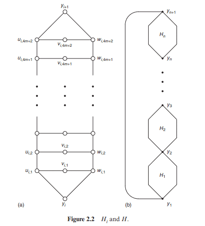
Lemma $5.16$ If $\mathcal{P}$ is a nontrivial monotone property of graphs of order $n=2^{m}$, then $D(\mathcal{P}) \geq n^{2} / 4$.
Proof. Let $H_{i}$ be the disjoint union of $2^{m-i}$ copies of the complete graph of order $2^{i}$. Then $H_{0} \subset H_{1} \subset \cdots \subset H_{m}=K_{n}$. Since $\mathcal{P}$ is nontrivial and is monotone, $H_{m}$ has the property $\mathcal{P}$ and $H_{0}$ does not have the property $\mathcal{P}$. Thus, there exists an index $j$ such that $H_{j+1}$ has the property $\mathcal{P}$ and $H_{j}$ does not have the property $\mathcal{P}$. Partition $H_{j}$ into two parts with vertex sets $A$ and $B$, respectively, each containing exactly $2^{m-j-1}$ disjoint copies of the complete graph of order $2^{j}$. Let $K_{A, B}$ be the complete bipartite graph between $A$ and $B$. Then $H_{j+1}$ is a subgraph of $H_{j} \cup K_{A, B}$. So, $H_{j} \cup K_{A, B}$ has the property $\mathcal{P}$. Now, let $f$ be the function on bipartite graphs between $A$ and $B$ such that $f$ has the value 1 at a bipartite graph $G$ between $A$ and $B$ if and only if $H_{j} \cup G$ has the property $\mathcal{P}$. Then $f$ is a nontrivial monotone weakly symmetric function with $|A| \cdot|B|\left(=2^{2 m-2}\right)$ variables. By Theorem $5.13, D(\mathcal{P}) \geq D(f)=2^{2 m-2}=n^{2} / 4$.
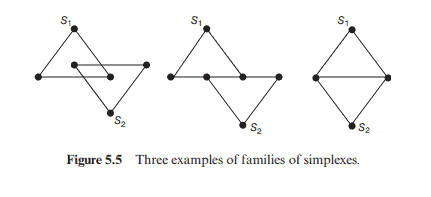
In this section, we introduce a powerful tool to study the elusiveness of monotone Boolean functions. We start with some concepts in topology. A triangle is a two-dimensional polygon with the minimum number of vertices. A tetrahedron is a three-dimensional polytope with the minimum number of vertices. They are the simplest polytopes with respect to the specific dimensions. They are both called simplexes. The concept of simplexes is a generalization of the notions of triangles and tetrahedrons. In general, a simplex is a polytope with the minimum number of vertices among all polytopes with certain dimension. For example, a point is a zero-dimensional simplex and a straight line segment is a one-dimensional simplex. The convex hull of linearly independent $n+1$ points in a Euclidean space is an $n$-dimensional simplex.
A face of a simplex $S$ is a simplex whose vertex set is a subset of vertices of $S$. A geometric simplicial complex is a family $\Gamma$ of simplexes satisfying the following conditions: (a) For $S \in \Gamma$, every face of $S$ is in $\Gamma$. (b) For $S, S^{\prime} \in \Gamma, S \cap S^{\prime}$ is a face for both $S$ and $S^{\prime}$. (c) For $S, S^{\prime} \in \Gamma, S \cap S^{\prime}$ is also a simplex in $\Gamma$. In Figure $5.5$, there are three examples; first two are not geometric simplicial complexes, the last one is.
Consider a set $X$ and a family $\Delta$ of subsets of $X . \Delta$ is called an (abstract) simplicial complex if for any $A$ in $\Delta$ every subset of $A$ also belongs to $\Delta$. Each member of $\Delta$ is called a face of $\Delta$. The dimension of a face $A$ is $|A|-1$. Any face of dimension 0 is called a vertex. For example, consider a set $X={a, b, c, d}$. The following family is a simplicial complex on $X$ : $$ \begin{aligned} \Delta=&{\emptyset,{a},{b},{c},{d},{a, b},{b, c},\ &{c, d},{d, a},{a, c},{a, b, c},{a, c, d}} \end{aligned} $$ The set ${a, b, c}$ is a face of dimension 2 and the empty set $\emptyset$ is a face of dimension $-1$.
Consider the class $\mathcal{C}$ of all subsets of ${0,1}^{*}$ and define subclasses $\mathcal{A}=\left{A \in \mathcal{C}: P^{A}=N P^{A}\right}$ and $B=\left{B \in \mathcal{C}: P^{B} \neq N P^{B}\right}$. One of the approaches to study the relativized $P=$ ? $N P$ question is to compare the two subclasses $\mathcal{A}$ and $\mathcal{B}$ to see which one is larger. In this subsection, we give a brief introduction to this study based on the probability theory on the space $\mathcal{C}$.
To define the notion of probability on the space $\mathcal{C}$, it is most convenient to identify each element $X \in \mathcal{C}$ with its characteristic sequence $\alpha_{X}=\chi_{X}(\lambda) \chi_{X}(0) \chi_{X}(1) \chi_{X}(00) \ldots$ (i.e., the $k$ th bit of $\alpha_{X}$ is 1 if and only if the $k$ th string of ${0,1}^{*}$, under the lexicographic ordering, is in $\left.X\right)$ and treat $\mathcal{C}$ as the set of all infinite binary sequences or, equivalently, the Cartesian product ${0,1}^{\infty}$. We can define a topology on $\mathcal{C}$ by letting the set ${0,1}$ have the discrete topology and forming the product topology on $\mathcal{C}$. This is the well-known Cantor space. We now define the uniform probability measure $\mu$ on $\mathcal{C}$ as the product measure of the simple equiprobable measure on ${0,1}$, that is, $\mu{0}=\mu{1}=1 / 2$. In other words, for any integer $n \geq 1$, the $n$th bit of a random sequence $\alpha \in \mathcal{C}$ has the equal probability to be 0 or 1 . If we identify each real number in $[0,1]$ with its binary expansion, then this measure $\mu$ is the Lebesgue measure on $[0,1] . .^{5}$
For any $u \in{0,1}^{}$, let $\Gamma_{u}$ be the set of all infinite binary sequences that begin with $u$, that is, $\Gamma_{u}^{u}=\left{u \beta: \beta \in{0,1}^{\infty}\right}$. Each set $\Gamma_{u}$ is called a cylinder. All cylinders $\Gamma_{u}, u \in{0,1}^{}$, together form a basis of open neighborhoods of the space $\mathcal{C}$ (under the product topology). It is clear that $\mu\left(\Gamma_{u}\right)=2^{-|u|}$ for all $u \in{0,1}^{}$. The smallest $\sigma$-field containing all $\Gamma_{u}$, for all $u \in{0,1}^{}$, is called the Borel field. ${ }^{6}$ Each set in the Borel field, called a Borel set, is measurable.
The question of which of the two subclasses $\mathcal{A}$ and $B$ is larger can be formulated, in this setting, as to whether $\mu(\mathcal{A})$ is greater than $\mu(\mathcal{B})$. In the following, we show that $\mu(\mathcal{A})=0$.
An important idea behind the proof is Kolmogorov’s zero-one law of tail events, which implies that if an oracle class is insensitive to a finite number of bit changes, then its probability is either zero or one. This property holds for the classes $\mathcal{A}$ and $B$ as well as most other interesting oracle classes.
数学代写|计算复杂度理论代写Computational complexity theory代考|Structure of Relativized NP
Although the meaning of relativized collapsing and relativized separation results is still not clear, many relativized results have been proven. These results show a variety of possible relations between the well-known complexity classes. In this section, we demonstrate some of these relativized results on complexity classes within $N P$ to show what the possible relations are between $P, N P, N P \cap \operatorname{co} N P$, and $U P$. The relativized results on the classes beyond the class $N P$, that is, those on $N P, P H$, and $P S P A C E$, will be discussed in later chapters.
The proofs of the following results are all done by the stageconstruction diagonalization. The proofs sometimes need to satisfy simultaneously two or more potentially conflicting requirements that make the proofs more involved. Theorem 4.20 (a) $(\exists A) P^{A} \neq N P^{A} \cap \operatorname{coN} P^{A} \neq N P^{A}$. (b) $(\exists B) P^{B} \neq N P^{B}=\cos P^{B}$. (c) $(\exists C) P^{C}=N P^{C} \cap \operatorname{coN} P^{C} \neq N P^{C}$. Proof. (a): This can be done by a standard diagonalization proof. We leave it as an exercise (Exercise 4.16(a)). (b): Let $\left{M_{i}\right}$ be an effective enumeration of all polynomial-time oracle DTMs and $\left{N_{i}\right}$ an effective enumeration of all polynomial-time oracle NTMs. For any set $B$, let $K_{B}=\left{\left\langle i, x, 0^{j}\right\rangle: N_{i}^{B}\right.$ accepts $x$ in $j$ moves $}$. Then, by the relativized proof of Theorem $2.11, K_{B}$ is $\leq_{m}^{P}$-complete for the class $N P^{B}$. Let $L_{B}=\left{0^{n}:(\exists x)|x|=n, x \in B\right}$. Then, it is clear that $L_{B} \in N P^{B}$. We are going to construct a set $B$ to satisfy the following requirements: $R_{0, t}$ : for each $x$ of length $t, x \notin K_{B} \Longleftrightarrow(\exists y,|y|=t) x y \in B$, $R_{1, i}:(\exists n) 0^{n} \in L_{B} \Longleftrightarrow M_{i}^{A}$ does not accept $0^{n} .$ Note that if requirements $R_{0, t}$ are satisfied for all $t \geq 1$, then $\overline{K_{B}} \in N P^{B}$ and, hence, $N P^{B}=\operatorname{coN} N P^{B}$, and if requirements $R_{1, i}$ are satisfied for all $i \geq 1$, then $L_{B} \notin P^{B}$ and, hence, $P^{B} \neq N P^{B}$.
We construct set $B$ by a stage construction. At each stage $n$, we will construct finite sets $B_{n}$ and $B_{n}^{\prime}$ such that $B_{n-1} \subseteq B_{n}, B_{n-1}^{\prime} \subseteq B_{n}^{\prime}$, and $B_{n} \cap$ $B_{n}^{\prime}=\emptyset$ for all $n \geq 1$. Set $B$ is define as the union of all $B_{n}, n \geq 0$.
The requirement $R_{0, t}, t \geq 1$, is to be satisfied by direct diagonalization at stage $2 t$. The requirements $R_{1, i}, i \geq 1$, are to be satisfied by a delayed diagonalization in the odd stages. We always try to satisfy the requirement $R_{1, i}$ with the least $i$ such that $R_{1, i}$ is not yet satisfied. We cancel an integer $i$ when $R_{1, i}$ is satisfied. Before stage 1 , we assume that $B_{0}=B_{0}^{\prime}=\emptyset$ and that none of integers $i$ is cancelled.
数学代写|计算复杂度理论代写Computational complexity theory代考|Graphs and Decision Trees
We first review the notion of graphs and the Boolean function representations of graphs. ${ }^{1}$ A graph is an ordered pair of disjoint sets $(V, E)$ such that $E$ is a set of pairs of elements in $V$ and $V \neq \emptyset$. The elements in the set $V$ are called vertices and the elements in the set $E$ are called edges. Two vertices are adjacent if there is an edge between them. Two graphs are isomorphic if there exists a one-to-one correspondence between their vertex sets that preserves adjacency.
A path is an alternating sequence of distinct vertices and edges starting and ending with vertices such that every vertex is an end point of its neighboring edges. The length of a path is the number of edges appearing in the path. A graph is connected if every pair of vertices are joined by a path.
Let $V={1, \ldots, n}$ be the vertex set of a graph $G=(V, E)$. Then its adjacency matrix $\left[x_{i j}\right]$ is defined by $$ x_{i j}= \begin{cases}1 & \text { if }{i, j} \in E, \ 0 & \text { otherwise. }\end{cases} $$ Note that $x_{i j}=x_{j i}$ and $x_{i i}=0$. So, the graph $G$ can be determined by $n(n-$ 1)/ 2 independent variables $x_{i j}, 1 \leq i<j \leq n$. For any property $\mathcal{P}$ of graphs with $n$ vertices, we define a Boolean function $f_{p}$ over $n(n-1) / 2$ variables $x_{i j}, 1 \leq i<j \leq n$, as follows: $$ f_{p}\left(x_{12}, \ldots, x_{n-1, n}\right)= \begin{cases}1 & \begin{array}{l} \text { if the graph } G \text { represented by }\left[x_{i, j}\right] \text { has } \ \text { the property } \mathcal{P} \end{array} \ 0 & \text { otherwise. }\end{cases} $$ Then $\mathcal{P}$ can be determined by $f_{p}$. For example, the property of connectivity corresponds to the Boolean functions $f_{\text {con }}$ of $n(n-1) / 2$ variables such that $f_{c o n}\left(x_{12}, \ldots, x_{n-1, n}\right)=1$ if and only if the graph $G$ represented by $\left[x_{i j}\right]$ is connected.
Not every Boolean function of $n(n-1) / 2$ variables represents a graph property because a graph property should be invariant under graph isomorphism. A Boolean function $f$ of $n(n-1) / 2$ variables is called a graph property if for every permutation $\sigma$ on the vertex set ${1, \ldots, n}$, $$ f\left(x_{12}, \ldots, x_{n-1, n}\right)=f\left(x_{\sigma(1) \sigma(2)}, \ldots, x_{\sigma(n-1) \sigma(n)}\right) \text {. } $$
First, a common view is that the question of whether $P$ is equal to $N P$ is a difficult question in view of Theorem 4.14. As most proof techniques developed in recursion theory, including the basic diagonalization and simulation techniques, relativize, any attack to the $P=$ ? NP question must use a new, unrelativizable proof technique. Many more contradictory relativized results like Theorem $4.14$ (including some in Section 4.8) on the relations between complexity classes tend to support this viewpoint. On the other hand, some unrelativizable proof techniques do exist in complexity theory. For instance, we will apply an algebraic technique to collapse the complexity class PSPACE to a subclass $I P$ (see Chapter 10). As there exists an oracle $X$ that separates $P S P A C E^{X}$ from $I P^{X}$, this proof is indeed unrelativizable. Though this is a breakthrough in the theory of relativization, it seems still too early to tell whether such techniques are applicable to a wider class of questions.
One of the most interesting topics in set theory is the study of independence results. A statement $A$ is said to be independent of a theory $T$ if there exist two models $M_{1}$ and $M_{2}$ of $T$ such that $A$ is true in $M_{1}$ and false in $M_{2}$. If a statement $A$ is known to be independent of the theory $T$, then neither $A$ nor its negation $\neg A$ is provable in theory $T$. The phenomenon of contradictory relativized results looks like a mini-independent result: neither the statement $P=N P$ nor its negation $P \neq N P$ is provable by relativizable techniques. This observation raises the question of whether they are provable within a formal proof system. In the following, we present a simple argument showing that this is indeed possible.
To prepare for this result, we first briefly review the concept of a formal proof system. An axiomatizable theory is a triple $F=(\Sigma, W, T)$, where $\Sigma$ is a finite alphabet, $W \subseteq \Sigma^{*}$ is a recursive set of well-formed formulas, and $T \subseteq W$ is an r.e. set. The elements in $T$ are called theorems. If $T$ is recursive, we say the theory $F$ is decidable. We are only interested in a sound theory in which we can prove the basic properties of TMs. In other words, we assume that TMs form a submodel for $F$, all basic properties of TMs are provable in $F$, and all theorems in $F$ are true in the TM model. In the following, we let $\left{M_{i}\right}$ be a fixed enumeration of multi-tape DTMs. Theorem 4.15 For any formal axiomatizable theory $F$ for which $T M s$ form a submodel, we can effectively find a DTM $M_{i}$ such that $L\left(M_{i}\right)=\emptyset$ and neither ” $P P^{L\left(M_{i}\right)}=N P^{L\left(M_{i}\right) “}$ nor ” $P^{L\left(M_{i}\right)} \neq N P^{L\left(M_{i}\right) “}$ is provable in $F$.
Proof. Let $A$ and $B$ be two recursive sets such that $P^{A}=N P^{A}$ and $P^{B} \neq$ $N P^{B}$. Define a TM $M$ such that $M$ accepts $(j, x)$ if and only if among the first $x$ proofs in $F$ there is a proof for the statement ” $P^{L\left(M_{j}\right)}=N P^{L\left(M_{j}\right)}$ ” and $x \in B$ or there is a proof for the statement ” $P^{L\left(M_{j}\right)} \neq N P^{L\left(M_{j}\right)}$ ” and $x \in A$. By the recursion theorem, there exists an index $j_{0}$ such that $M_{j_{0}}$ accepts $x$ if and only if $M$ accepts $\left(j_{0}, x\right)$. (See, e.g., Rogers (1967) for the recursion theorem.)
Now, if there is a proof for the statement ” $P^{L\left(M_{k b}\right)}=N P^{L\left(M_{k}\right)}$ ” in $F$, then for almost all $x, M$ accepts $\left(j_{0}, x\right)$ if and only if $x \in B$. That is, the set $L\left(M_{j_{0}}\right)$ differs from the set $B$ by only a finite set and, hence, $P^{B} \neq N P^{B}$ implies $P^{L\left(M_{f 0}\right)} \neq N P^{L\left(M_{j 0}\right)}$. Similarly, if there exists a proof for the statement ” $P^{L\left(M_{j 0}\right)} \neq N P^{L\left(M_{f 0}\right)}$ “, then $L\left(M_{j_{0}}\right)$ differs from $A$ by only a finite set theory $F$, we conclude that neither ” $P^{L\left(M_{f 0}\right)}=N P^{L\left(M_{j 0}\right) “}$ nor ” $P^{L\left(M_{f 0}\right)} \neq$ $N P^{L\left(M_{f 0}\right)}$, , is provable in $F$.
Furthermore, because neither ” $P^{L\left(M_{f 0}\right)}=N P^{L\left(M_{f 0}\right)}$ ” nor ” $P^{L\left(M_{f 0}\right)} \neq$ $N P^{L\left(M_{j_{0}}\right) \text { ” }}$ is provable in $F$, the machine $M_{j_{0}}$ does not accept any input $x$, that is, $L\left(M_{j_{0}}\right)=\emptyset$.
Still another viewpoint is that the formulation of the relativized complexity class $N P^{A}$ used in Theorem $4.14$ does not reflect correctly the concept of nondeterministic computation. Consider the set $L_{B}$ in the proof of Theorem 4.14. Note that although each computation path of the oracle NTM $M$ that accepts $L_{B}$ asks only one question to determine whether $0^{n}$ is in $B$, the whole computation tree of $M^{B}(x)$ makes an exponential number of queries. While it is recognized that this is the distinctive property of an NTM to make, in the whole computation tree, an exponential number of moves, the fact that $M$ can access an exponential amount of information about the oracle $B$ immediately makes the oracle NTMs much stronger than oracle DTMs. To make the relation between oracle NTMs and oracle DTMs close to that between regular NTMs and regular DTMs, we must not allow the oracle NTMs to make arbitrary queries. Instead, we would like to know whether an oracle NTM that is allowed to make, in the whole computation tree, only a polynomial number of queries is stronger than an oracle DTM. When we add these constraints to the oracle NTMs, it turns out that the relativized $P=$ ?NP question is equivalent to the unrelativized version. This result supports the viewpoint that the relativized separation of Theorem $4.14$ is due to the extra information that an oracle NTM can access, rather than the nondeterminism of the NTM and, hence, this kind of separation results bear no relation to the original unrelativized questions. This type of relativization is called positive relativization. We present a simple result of this type in the following.
数学代写|计算复杂度理论代写Computational complexity theory代考|Incomplete Problems in NP
We have seen many $N P$-complete problems in Chapter 2. Many natural problems in $N P$ turn out to be $N P$-complete. There are, however, a few interesting problems in $N P$ that are not likely to be solvable in deterministic polynomial time but also are not known to be $N P$-complete. The study of these problems is thus particularly interesting, because it not only can classify the inherent complexity of the problems themselves but can also provide a glimpse of the internal structure of the class $N P$. We start with some examples.
Example 4.1 GRAPH ISOMORPHISM (GIso): Given two graphs $G_{1}=$ $\left(V_{1}, E_{1}\right)$ and $G_{2}=\left(V_{2}, E_{2}\right)$, determine whether they are isomorphic, that is, whether there is a bijection $f: V_{1} \rightarrow V_{2}$ such that ${u, v} \in E_{1}$ if and only if ${f(u), f(v)} \in E_{2}$.
The problem SuBGRAPH IsomORPHISM, which asks whether a given graph $G_{1}$ is isomorphic to a subgraph of another given graph $G_{2}$, can be proved to be $N P$-complete easily. However, the problem GIso is neither known to be $N P$-complete nor known to be in $P$, despite extensive studies in recent years. We will prove in Chapter 10, through the notion of interactive proof systems, that GIso is not $N P$-complete unless the polynomial-time hierarchy collapses to the level $\Sigma_{2}^{P}$. This result suggests that GIso is probably not $N P$-complete.
There are many number-theoretic problems in $N P$ that are neither known to be $N P$-complete nor known to be in $P$. We list three of them that have major applications in cryptography. An integer $x \in \mathbb{Z}{n}^{}$ is called a quadratic residue modulo $n$ if $x \equiv y^{2} \bmod n$ for some $y \in \mathbb{Z}{n}^{}$. We write $x \in Q R_{n}$ to denote this fact.
数学代写|计算复杂度理论代写Computational complexity theory代考|One-Way Functions and Cryptography
One-way functions are a fundamental concept in cryptography, having a number of important applications, including public-key cryptosystems,pseudorandom generators, and digital signatures. Intuitively, a one-way function is a function that is easy to compute but its inverse is hard to compute. Thus it can be applied to develop cryptosystems that need easy encoding but difficult decoding. If we identify the intuitive notion of “easiness” with the mathematical notion of “polynomial-time computability,” then one-way functions are subproblems of $N P$, because the inverse function of a polynomial-time computable function is computable in polynomial-time relative to an oracle in $N P$, assuming that the functions are polynomially honest. Indeed, all problems in $N P$ may be viewed as one-way functions.
Example 4.5 Define a function $f_{\mathrm{SAT}}$ as follows: For each Boolean function $F$ over variables $x_{1}, \ldots, x_{n}$ and each Boolean assignment $\tau$ on $x_{1}, \ldots, x_{n}$ $$ f_{\mathrm{SAT}}(F, \tau)= \begin{cases}\langle F, 1\rangle & \text { if } \tau \text { satisfies } F, \ \langle F, 0\rangle & \text { otherwise. }\end{cases} $$ It is easily seen that $f_{\text {SAT }}$ is computable in polynomial time. Its inverse mapping $\langle F, 1\rangle$ to $\langle F, \tau\rangle$ is exactly the search problem of finding a truth assignment for a given Boolean formula. Using the notion of polynomialtime Turing reducibility and the techniques developed in Chapter 2, we can see that the inverse function of $f_{\mathrm{SAT}}$ is polynomial-time equivalent to the decision problem SAT. Thus, the inverse of $f_{\mathrm{SAT}}$ is not polynomial-time computable if $P \neq N P$.
Strictly speaking, function $f_{\mathrm{SAT}}$ is, however, not really a one-way function because it is not a one-to-one function and its inverse is really a multivalued function. In the following, we define one-way functions for one-to-one functions. We say that a function $f: \Sigma^{} \rightarrow \Sigma^{}$ is polynomially honest if there is a polynomial function $q$ such that for each $x \in \Sigma^{*}$, $|f(x)| \leq q(|x|)$ and $|x| \leq q(|f(x)|)$.
The concept of relativization originates from recursive function theory. Consider, for example, the halting problem. We may formulate it in the following form: $K=\left{x \mid M_{x}(x)\right.$ halts $}$, where $M_{x}$ is the $x$ th TM in a standard enumeration of all TMs. Now, if we consider all oracle TMs, we may ask whether the set $K_{A}=\left{x \mid M_{x}^{A}(x)\right.$ halts $}$ is recursive relative to $A$. This is the halting problem relative to set $A$. It is easily seen from the original proof for the nonrecursiveness of $K$ that $K_{A}$ is nonrecursive relative to $A$ (i.e., no oracle TM can decide $K_{A}$ using $A$ as an oracle). Indeed, most results in recursive function theory can be extended to hold relative to any oracle set. We say that such results relativize. In this section, we investigate the problem of whether $P=N P$ in the relativized form. First, we need to define what is meant by relativizing the question of whether $P=N P$. For any set $A$, recall that $P^{A}(\circ r P(A))$ is the class of sets computable in polynomial time by oracle DTMs using $A$ as the oracle and, similarly, NPA (or $N P(A))$ is the class of sets accepted in polynomial time by oracle NTMs classes $P$ and $N P$, we show that the relativized $P=? N P$ question has both the positive and negative answers, depending on the oracle set $A$. Theorem $4.14$ (a) There exists a recursive set $A$ such that $P^{A}=N P^{A}$. (b) There exists a recursive set $B$ such that $P^{B} \neq N P^{B}$. Proof. (a): Let $A$ be any set that is $\leq_{m}^{P}$-complete for PSPACE. Then, by Savitch’s theorem, we have $$ N P^{A} \subseteq N P S P A C E=P S P A C E \subseteq P^{A} . $$
The polynomial-time hierarchy was formally defined by oracle TMs. As the oracles play a mysterious role in the computation of an oracle TM, it is relatively more difficult to analyze the computation of such machines. The characterization of Theorem $3.8$ provides a different view, and it has been found useful for many applications. In this section, we formalize this characterization as a computational model, called the alternating Turing machine (abbreviated as ATM), that can be used to define the complexity classes in the polynomial-time hierarchy without using the notion of oracles.
An ATM $M$ is an ordinary NTM with its states partitioned into two subsets, called the universal states and the existential states. An ATM operates exactly the same as an NTM, but the notion of its acceptance of an input is defined differently. Thus, the computation of an ATM $M$ is a computation tree of configurations with each pair $(\alpha, \beta)$ of parent and child configurations satisfying $\alpha \vdash_{M} \beta$. We say a configuration is a universal configuration if it is in a universal state, and it is an existential configuration if it is in an existential state.
To define the notion of an ATM accepting an input, we assign, inductively, the label ACCEPT to some of the nodes in this computation tree as follows: A leaf is labeled ACCEPT if and only if it is in the accepting state. An internal node in the universal state is labeled with ACCEPT if and only if all of its children are labeled with ACCEPT. An internal node in the existential state is labeled with ACCEPT if and only if at least one of its children is labeled with ACCEPT. We say an ATM M accepts an input $x$ if the root of the computation tree is labeled with ACCEPT using the above labeling system. Thus an NTM is just an ATM in which all states are classified as existential states.
When an NTM $M$ accepts an input $x$, an accepting computation path is a witness to this fact. Also, we define time $_{M}(x)$ to be the length of a shortest accepting path. For an ATM $M$, to demonstrate that it accepts an input $x$, we need to display the accepting computation subtree $T_{a c c}$ of the computation tree $T$ of $M(x)$ that has the following properties: (i) The root of $T$ is in $T_{a c c}$. (ii) If $u$ is an internal existential node in $T_{a c c}$, then exactly one child of $u$ in $T$ is in $T_{a c c}$.
Our first PSPACE-complete problem is the space-bounded halting problem (SBHP). SPACE Bounded Halting Problem (SBHP): Given a DTM $M$, an input $x$, and an integer $s$, written in the unary form $0^{s}$, determine whether $M$ accepts $x$ within space bound $s$. Theorem 3.23 SBHP is $\leq_{m}^{P}$-complete for PSPACE. Proof. The proof is similar to that of Theorem 2.11. The existence of a PSPACE-complete set implies that if the polynomial-time hierarchy is properly infinite, then PSPACE properly contains $P H$.
Theorem 3.24 If $P H=P S P A C E$, then the polynomial-time hierarchy collapses to $\Sigma_{k}^{P}$ for some $k>0$.
Proof. If $P H=P S P A C E$, then SBHP $\in P H=\bigcup_{k \geq 0} \Sigma_{k}^{P}$ and, hence, SBHP $\in \Sigma_{k}^{P}$ for some $k \geq 0$. This implies that PSPACE $\subseteq \Sigma_{k}^{P}$, because $\Sigma_{k}^{P}$ is closed under the $\leq_{m}^{P}$-reducibility.
The first natural PSPACE-complete problem is a generalization of $S A T_{k}$. The inputs to this problem are Boolean formulas with quantifiers $(\exists x)$ and $(\forall x)$. An occurrence of a variable $v$ in a Boolean formula $F$ is a bounded variable if there is a quantifier $(\exists v)$ or $(\forall v)$ in $F$ such that this occurrence of $v$ is in the scope of the quantifier. A Boolean formula $F$ is called a quantified Boolean formula if every occurrence of every variable in $F$ is a bounded variable. For instance, $F=(\forall x)[(\forall y)[(\exists z)[x \bar{y} z+\bar{x} y \bar{z}] \rightarrow(\exists z)[(x \bar{z}+\bar{x} z)(y \bar{z}+\bar{y} z)]]]$ is a quantified Boolean formula. In the above, we used brackets […] to denote the scope of a quantifier and $\rightarrow$ to denote the Boolean operation $(a \rightarrow b)=(\bar{a}+b)$. Each quantified Boolean formula has a normal form in which all quantifiers occur before any occurrence of a Boolean variable, and the scope of each quantifier is the rest of the formula to its right. For instance, the normal form (with renaming) of the above formula $F$ is $(\forall x)(\forall y)(\forall z)(\exists w)[(x \bar{y} z+\bar{x} y \bar{z}) \rightarrow((x \bar{w}+\bar{x} w)(y \bar{w}+\bar{y} w))]$ QUANTIFIED BOOLEAN FORMULA (QBF): Given a quantified Boolean formula $F$, determine whether $F$ is true.
All complete problems studied so far are candidates for intractable problems, but their intractability still depends on the separation of the classes $N P, P S P A C E$, and $P H$ from the class $P$. Are there natural problems that are provably intractable in the sense that they can be proved not belonging to $P$ ? In this section, we present a few problems that are complete for $E X P$ and, hence, not in $P$.
Our first $E X P$-complete problem is the bounded halting problem on deterministic machines with the time bound encoded in binary form. EXPONENTIAL-Time BoUnDEd HALTING PROBLEM (EXP-BHP): Given a DTM $M$, a string $x$, and an integer $n>0$, written in the binary form, determine whether $M(x)$ halts in $n$ moves. Proposition 3.30 EXP-BHP is EXP-complete. Proof. If $L$ is accepted by a DTM $M$ in time $2^{c n}$, then the function $f(x)=$ $\left\langle M, x, 2^{c|x|}\right\rangle$ is a polynomial-time reduction from $L$ to ExP-BHP.
We note that in the above problem, if the time bound $n$ is written in the unary form (as in the problem BHP), then the problem becomes polynomial-time solvable. Indeed, there is a simple translation of most $P$-complete problems ${ }^{1}$ to $E X P$-complete problems by more succinct encodings of the inputs. In the following, we demonstrate this idea on the famous $P$-complete problem, CIRCUIT VALUE Problem (CVP).
Let $C$ be a Boolean circuit ${ }^{2}$ satisfying the following property: $C$ has $n$ gates numbered from 1 to $n$; we let $C(i)$ denote the gate of $C$ numbered $i$. There are four types of gates in circuit $C$ : ZERO gates, ONE gates, AND gates, and OR gates. A ZERO (ONE) gate has no input and one output whose value is 0 (1, respectively). An AND (OR) gate has two inputs and one output whose value is the Boolean product (Boolean sum, respectively) of the two inputs. If the gate $i$ is an AND or OR gate, then its two inputs are the outputs of two gates whose numbers are lower than $i$. Note that this circuit $C$ does not have input gates and so it computes a unique Boolean value (the output of gate $n$ ). If the circuit is given explicitly, then its output value is computable in polynomial time. (In fact, it is $P$-complete; see Theorem 6.41). In the following, we consider the encoding of the circuit by a DTM. We say that a DTM $M$ generates a circuit $C$ of size $n$ in time $m$ if for all $i, 0 \leq i \leq n, M(i)$ outputs a triple $\langle b, j, k\rangle$ in $m$ moves, with $0 \leq b \leq 3$ and $1 \leq j, k<i$ if $b \leq 1$, such that (i) If $b=0$, then $C(i)=C(j) \cdot C(k)$; (ii) If $b=1$, then $C(i)=C(j)+C(k)$; (iii) If $b=2$, then $C(i)=0$; (iv) If $b=3$, then $C(i)=1$.
Based on the notion of polynomial-time Turing reducibility, we can see that many important combinatorial optimization problems are $N P$-hard search problems. We prove these results by first showing that the corresponding decision problems are $\leq_{m}^{P}$-complete for $N P$ and then proving that the problems of searching for the optimum solutions are $\leq_{T}^{P}$-equivalent to the corresponding decision problems. In practice, however, we often do not need the optimum solution. A nearly optimum solution is sufficient for most applications. In general, the $N P$-hardness of the optimization problem does not necessarily imply the $N P$-hardness of the approximation to the optimization problem. In this section, we demonstrate that for some $N P$-complete optimization problems, their approximation versions are also $N P$-hard and, yet, for some problems, polynomial-time approximation is achievable. These types of results are often more difficult to prove than other $N P$-completeness results. We only present some easier results and delay the more involved results until Chapter $11 .$
We first introduce a general framework to deal with the approximation problems. Very often, an optimization problem $\Pi$ has the following general structure: for each input instance $x$ to the problem $\Pi$, there are a number of solutions $y$ to $x$. For each solution $y$, we associate a value $v_{\Pi}(y)$ (or, simply, $v(y)$, if $\Pi$ is known from the context) to it. The problem $\Pi$ is to find, for the given input $x$, a solution $y$ to $x$ such that its value $v(y)$ is maximized (or minimized). For instance, we can fit the problem MAXCLIQUE into this framework as follows: an input to the problem is a graph $G$; a solution to $G$ is a clique $C$ in $G$; the value $v(C)$ of a solution $C$ is the number of its vertices; and the problem is to find, for a given graph $G$, a clique of the maximum size.
Let $r$ be a real number with $r>1$. For a maximization problem $\Pi$ with the above structure, we define its approximation version, with the approximation ratio $r$, as follows: $r$-APProx-П: For a given input $x$, find a solution $y$ to $x$ such that $v(y) \geq v^{}(x) / r$, where $v^{}(x)=\max {v(z): z$ is a solution to $x$. Similarly, for a minimization problem $\Pi$, its approximation version with the approximation ratio $r$ is as follows:$r$-APPROX-П: For a given input $x$, find a solution $y$ to $x$ such that $v(y) \leq r \cdot v^{}(x)$, where $v^{}(x)=\min {v(z): z$ is a solution to $x}$.
We have defined in Chapter 2 the notions of polynomial-time Turing reducibility and oracle TMs, and have seen that many optimization problems, when formulated in the search problem form, are solvable in polynomial time relative to a set in $N P$. We now extend this notion to nondeterministic oracle TMs and study problems that are solvable in nondeterministic polynomial time relative to sets in $N P$.
A nondeterministic (function-)oracle Turing machine (oracle NTM) is an NTM equipped with an additional query tape and two additional states: the query state and the answer state. The computation of an oracle NTM is similar to that of an oracle DTM, except that at each nonquery state an oracle NTM can make a nondeterministic move. We require that the query step of the computation be a deterministic move determined by the oracle. Let $M$ be an oracle NTM and $f$ an oracle function. We write $M^{f}(x)$ to denote the computation of $M$ on input $x$, using $f$ as the oracle function (note that this is a computation tree). If the oracle function is a characteristic function of a set $A$, we say $M$ is a set-oracle NTM and write $M^{A}$ to denote $M^{f}$, and write $L(M, A)$ to denote the set of strings accepted by $M^{A}$.
The time complexity of a set-oracle NTM is also defined similar to that of a set-oracle DTM. In particular, the actions from the query state to the answer state count as only one step. For any fixed oracle set $A$, we let $\operatorname{time}{M}^{A}(x)$ be the length of the shortest accepting computation path of $M^{A}(x)$ and $t{M}^{A}(n)=\max \left({n+1} \cup\left{\operatorname{time}{M}^{A}(x):|x|=n, M^{A}\right.\right.$ accepts $\left.\left.x\right}\right)$. For a set-oracle NTM $M$, we say $t{M}(n)$ is bounded by a function $g(n)$, if for all oracle sets $A, t_{M}^{A}(n) \leq g(n)$. An oracle NTM $M$ is a polynomialtime oracle $N T M$ if $t_{M}(n)$ is bounded by a polynomial function $p$. Let $A$ be a set and $\mathcal{C}$ be a complexity class. We let $N P^{A}$ denote the class of sets accepted by polynomial-time oracle NTMs relative to the oracle $A$, and let $N P^{C}$ (or, $N P(\mathcal{C})$ ) denote the class of sets accepted by polynomial-time oracle NTMs using an oracle $B \in \mathcal{C}$ (i.e., $N P^{C}=\bigcup_{B \in C} N P^{B}$ ).
The polynomial-time hierarchy is the polynomial analog of the arithmetic hierarchy in recursion theory (Rogers, 1967). It can be defined inductively by oracle NTMs.
Definition $3.3$ For integers $n \in \mathbb{N}$, complexity classes $\Delta_{n}^{P}$, $\Sigma_{n}^{P}$, and $\Pi_{n}^{P}$ are defined as follows: $$ \begin{aligned} \Sigma_{0}^{P} &=\Pi_{0}^{P}=\Delta_{0}^{P}=P, \ \Sigma_{n+1}^{P} &=N P\left(\Sigma_{n}^{P}\right), \ \Pi_{n+1}^{P} &=c o-\Sigma_{n+1}^{P}, \ \Delta_{n+1}^{P} &=P\left(\Sigma_{n}^{P}\right), \quad n \geq 0 . \end{aligned} $$ The class $P H$ is defined to be the union of $\Sigma_{n}^{P}$ over all $n \geq 0$. Thus, $\Sigma_{1}^{P}=N P, \Sigma_{2}^{P}=N P^{N P}, \Sigma_{3}^{P}=N P\left(N P^{N P}\right)$, and so on. It is easy to verify that these classes form a hierarchy. Proposition 3.4 For all $k>0$, $$ \Sigma_{k}^{P} \cup \Pi_{k}^{P} \subseteq \Delta_{k+1}^{P} \subseteq \Sigma_{k+1}^{P} \cap \Pi_{k+1}^{P} \subseteq P S P A C E . $$ Proof. Note that $P^{A}=P^{\bar{A}}$, and so $\Pi_{k}^{P} \subseteq P\left(\Pi_{k}^{P}\right)=P\left(\Sigma_{k}^{P}\right)=\Delta_{k+1}^{P}$. Other inclusive relations among classes in $P H$ follow easily from the definition. Finally, the whole hierarchy $P H$ is included in $P S P A C E$ following from Proposition 3.2(b).
Based on the above proposition, we show in Figure $3.1$ the basic structure of the polynomial-time hierarchy. To further understand the structure of the polynomial-time hierarchy, we first extend Theorem $2.1$ to a characterization of the polynomial-time hierarchy in terms of the polynomiallength-bounded quantifiers.
First, we observe some closure properties of the polynomial-time hierarchy under the Boolean operations.
The notion of reducibilities was first developed in recursion theory. In general, a reducibility $\leq_{r}$ is a binary relation on languages that satisfies the reflexivity and transitivity properties and, hence, it defines a partial ordering on the class of all languages. In this section, we introduce the notion of polynomial-time many-one reducibility. Let $A \subseteq \Sigma^{}$ and $B \subseteq \Gamma^{}$ be two languages. We say that $A$ is many-one reducible to $B$, denoted by $A \leq_{m} B$, if there exists a computable function $f: \Sigma^{} \rightarrow \Gamma^{}$ such that for each $x \in \Sigma^{*}, x \in A$ if and only if $f(x) \in B$. If the reduction function $f$ is further known to be computable in polynomial time, then we say that $A$ is polynomial-time many-one reducible to $B$ and write $A \leq_{m}^{P} B$. It is easy to see that polynomial-time many-one reducibility does satisfy the reflexivity and transitivity properties and, hence, indeed is a reducibility. Proposition $2.8$ The following hold for all sets $A, B$, and $C$ : (a) $A \leq_{m}^{P} A$ (b) $A \leq_{m}^{P} B, B \leq_{m}^{P} C \Rightarrow A \leq_{m}^{P} C$. Note that if $A \leq_{m}^{P} B$ and $B \in P$, then $A \in P$. In general, we say a complexity class $\mathcal{C}$ is closed under the reducibility $\leq_{r}$ if $A \leq_{r} B$ and $B \in \mathcal{C}$ imply $A \in \mathcal{C}$
Proposition 2.9 The complexity classes $P, N P$, and PSPACE are all closed under $\leq_{m}^{P}$
Note that the complexity class $E X P=\bigcup_{c>0} D T I M E\left(2^{c n}\right)$ is not closed under $\leq_{m}^{P}$. People sometimes, therefore, study a weaker class of exponential-time computable sets EXPPOLY = $\bigcup_{k>0} D T I M E\left(2^{n^{k}}\right)$, which is closed under $\leq_{m}^{P}$.
For any complexity class $\mathcal{C}$ that is closed under a reducibility $\leq_{r}$, we say a set $B$ is $\leq_{r}$ hard for class $C$ if $A \leq_{r} B$ for all $A \in \mathcal{C}$ and we say a set $B$ is $\leq_{r}-$ complete for class $\mathcal{C}$ if $B \in \mathcal{C}$ and $B$ is $\leq_{r}$-hard for $\mathcal{C}$. For convenience, we say a set $B$ is $\mathcal{C}$-complete if $B$ is $\leq_{m}^{P}$-complete for the class $\mathcal{C}$. $^{2}$ Thus, a set $B$ is $N P$-complete if $B \in N P$ and $A \leq_{m}^{P} B$ for all $A \in N P$. An $N P$-complete set $B$ is a maximal element in $N P$ under the partial ordering $\leq_{m}^{P}$. Thus, it is not in $P$ if and only if $P \neq N P$.
The importance of the notion of $N P$-completeness is witnessed by thousands of $N P$-complete problems from a variety of areas in computer science, discrete mathematics, and operations research. Theoretically, all these problems can be proved to be $N P$-complete by reducing SAT to them. It is practically much easier to prove new $N P$-complete problems from some other known $N P$-complete problems that have similar structures as the new problems. In this section, we study some best-known $N P$-complete problems that may be useful to obtain new $N P$-completeness results. VERTEX COVER (VC): Given a graph $G=(V, E)$ and an integer $K \geq 0$, determine whether $G$ has a vertex cover of size at most $K$, that is, determine whether $V$ has a subset $V^{\prime}$ of size $\leq K$ such that each $e \in E$ has at least one end point in $V^{\prime}$. Theorem 2.14 VC is NP-complete. Proof. It is easy to see that $\mathrm{VC}$ is in $N P$. To show that $\mathrm{VC}$ is complete for $N P$, we reduce 3-SAT to it.
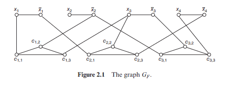
Let $F$ be a 3-CNF formula with $m$ clauses $C_{1}, C_{2}, \ldots, C_{m}$ over $n$ variables $x_{1}, x_{2}, \ldots, x_{n}$. We construct a graph $G_{F}$ of $2 n+3 m$ vertices as follows. The vertices are named $x_{i}, \bar{x}{i}$ for $1 \leq i \leq n$, and $c{j k}$ for $1 \leq j \leq m$, $1 \leq k \leq 3$. The vertices are connected by the following edges: for each $i, 1 \leq i \leq n$, there is an edge connecting $x_{i}$ and $\bar{x}{i}$; for each $j, 1 \leq j \leq m$, there are three edges connecting $c{j, 1}, c_{j, 2}, c_{j, 3}$ into a triangle and, in addition, if $C_{j}=\ell_{1}+\ell_{2}+\ell_{3}$, then there are three edges connecting each $c_{j, k}$ to the vertex named $\ell_{k}, 1 \leq k \leq 3$. Figure $2.1$ shows the graph $G_{F}$ for $F=\left(x_{1}+\bar{x}{2}+x{3}\right)\left(\bar{x}{1}+x{3}+\bar{x}{4}\right)\left(\bar{x}{2}+\bar{x}{3}+x{4}\right) .$
We claim that $F$ is satisfiable if and only if $G_{F}$ has a vertex cover of size $n+2 m$. First, suppose that $F$ is satisfiable by a truth assignment $\tau$. Let $S_{1}=\left{x_{i}: \tau\left(x_{i}\right)=1,1 \leq i \leq n\right} \cup\left{\bar{x}{i}: \tau\left(x{i}\right)=0,1 \leq i \leq n\right}$. Next for each $j, 1 \leq j \leq m$, let $c_{j, j}$ be the vertex of the least index $j_{k}$ such that $c_{j, j_{k}}$ is adjacent to a vertex in $S_{1}$. (By the assumption that $\tau$ satisfies $F$, such an index $j_{k}$ always exists.) Then, let $S_{2}=\left{c_{j, r}: 1 \leq r \leq 3, r \neq j_{k}, 1 \leq j \leq\right.$ $m}$ and $S=S_{1} \cup S_{2}$. It is clear that $S$ is a vertex cover for $G_{F}$ of size $n+2 m$
Conversely, suppose that $G_{F}$ has a vertex cover $S$ of size at most $n+$ $2 m$. As each triangle over $c_{j_{1}}, c_{j_{2}}, c_{j_{3}}$ must have at least two vertices in $S$ and each edge $\left{x_{i}, \bar{x}{i}\right}$ has at least one vertex in $S, S$ is of size exactly $n+2 m$ with exactly two vertices from each triangle $c{j_{1}}, c_{j_{2}}, c_{j_{3}}$ and exactly one vertex from each edge $\left{x_{i}, \bar{x}{i}\right}$. Define $\tau\left(x{i}\right)=1$ if $x_{i} \in S$ and $\tau\left(x_{i}\right)=0$ if $\bar{x}{i} \in S$. Then, each clause $C{j}$ must have a true literal which is the one adjacent to the vertex $c_{j, k}$ that is not in $S$. Thus, $F$ is satisfied by $\tau$.
The above construction is clearly polynomial-time computable. Hence, we have proved 3-SAT $\leq_{m}^{P} V$ VC.
Polynomial-time many-one reducibility is a strong type of reducibility on decision problems (i.e., languages) that preserves the membership in the class $P$. In this section, we extend this notion to a weaker type of reducibility called polynomial-time Turing reducibility that also preserves the membership in $P$. Moreover, this weak reducibility can also be applied to search problems (i.e., functions).
Intuitively, a problem $A$ is Turing reducible to a problem $B$, denoted by $A \leq_{T} B$, if there is an algorithm $M$ for $A$ which can ask, during its computation, some membership questions about set $B$. If the total amount of time used by $M$ on an input $x$, excluding the querying time, is bounded by $p(|x|)$ for some polynomial $p$, and furthermore, if the length of each query asked by $M$ on input $x$ is also bounded by $p(|x|)$, then we say $A$ is polynomial-time Turing reducible to $B$ and denote it by $A \leq_{T}^{P} B$. Let us look at some examples.
Example $2.20$ (a) For any set $A, \bar{A} \leq_{T}^{P} A$, where $\bar{A}$ is the complement of $A$. This is achieved easily by asking the oracle $A$ whether the input $x$ is in $A$ or not and then reversing the answer. Note that if $N P \neq \operatorname{coNP}$, then $\overline{\mathrm{SAT}}$ is not polynomial-time many-one reducible to SAT. So, this demonstrates that the $\leq_{T}^{P}$-reducibility is potentially weaker than the $\leq_{m}^{P}$-reducibility (cf. Exercise $2.14$ ). (b) Recall the $N P$-complete problem CLIQUE. We define a variation of the problem CLIQUE as follows: EXACT-CLIQUE: Given a graph $G=(V, E)$ and an integer $K \geq$ 0 , determine whether it is true that the maximum-size clique of $G$ is of size $K$. It is not clear whether EXACT-CLIQUE is in $N P$. We can guess a subset $V^{\prime}$ of $V$ of size $K$ and verify in polynomial time that the subgraph of $G$ induced by $V^{\prime}$ is a clique. However, there does not seem to be a nondeterministic algorithm that can check that there is no clique of size greater than $K$ in polynomial time. Therefore, this problem may seem even harder
than the $N P$-complete problem CLIQUE. In the following, however, we show that this problem is actually polynomial-time equivalent to CLIQUE in the sense that they are polynomial-time Turing reducible to each other. Thus, either they are both in $P$ or they are both not in $P$.
First, let us describe an algorithm for the problem CLIQUE that can ask queries to the problem EXACT-CLIQUE. Assume that $G=(V, E)$ is a graph and $K$ is a given integer. We want to know whether there is a clique in $G$ that is of size $K$. We ask whether $(G, k)$ is in EXACT-CLIQUE for each $k=1,2, \ldots,|V|$. Then, we will get the maximum size $k^{}$ of the cliques of $G$. We answer YES to the original problem CLIQUE if and only if $K \leq k^{}$.
Conversely, let $G=(V, E)$ be a graph and $K$ a given integer. Note that the maximum clique size of $G$ is $K$ if and only if $(G, K) \in$ CLIQUE and $(G, K+1) \notin$ CLIQUE. Thus, the question of whether $(G, K) \in$ ExACTCLIQUE can be solved by asking two queries to the problem CLIQUE. (See Exercise 3.3(b) for more studies on EXACT-CLIQUE.)