数学代写|概率论代写Probability theory代考|STAT414
如果你也在 怎样代写概率论Probability Theory 这个学科遇到相关的难题,请随时右上角联系我们的24/7代写客服。概率论Probability Theory是研究与随机现象有关的概率的数学分支。一个随机现象可能有几种结果。概率论用一定的形式概念描述某一特定结果发生的几率。
概率论Probability Theory某些随机变量在概率论中经常出现,因为它们很好地描述了许多自然或物理过程。因此,它们的分布在概率论中具有特殊的重要性。一些基本的离散分布有离散均匀分布、伯努利分布、二项式分布、负二项式分布、泊松分布和几何分布。重要的连续分布包括连续均匀分布、正态分布、指数分布、分布和分布。
statistics-lab™ 为您的留学生涯保驾护航 在代写概率论Probability theory方面已经树立了自己的口碑, 保证靠谱, 高质且原创的统计Statistics代写服务。我们的专家在代写概率论Probability theory代写方面经验极为丰富,各种代写概率论Probability theory相关的作业也就用不着说。

数学代写|概率论代写Probability theory代考|EXAMPLES AND APPLICATIONS
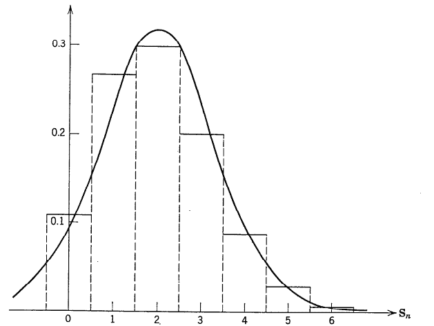
(a) Binomial distribution. Let $\mathbf{S}_n$ be the number of successes in $n$ Bernoulli trials with probability $p$ for success. We know that $\mathbf{S}_n$ has the binomial distribution ${b(k ; n, p)}$, whence $\mathbf{E}\left(\mathbf{S}_n\right)=\sum k b(k ; n, p)=$ $=n p \sum b(k-1 ; n-1, p)$. The last sum includes all terms of the binomial distribution for $n-1$ and hence equals 1 . Therefore the mean of the binomial distribution is
$$
\mathbf{E}\left(\mathbf{S}_n\right)=n p .
$$
The same result could have been obtained without calculation by a method which is often expedient. Let $\mathbf{X}_k$ be the number of successes scored at the $k$ th trial. This random variable assumes only the values 0 and 1 with corresponding probabilities $q$ and $p$. Hence
$$
\mathbf{E}\left(\mathbf{X}_k\right)=0 \cdot q+1 \cdot p=p
$$
and since
$$
\mathrm{S}_n=\mathbf{X}_1+\mathbf{X}_2+\cdots+\mathbf{X}_n
$$
we get (3.1) directly from (2.4).
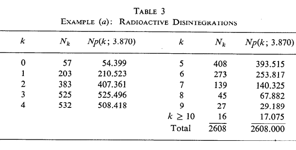
(b) Poisson distribution. If $\mathbf{X}$ has the Poisson distribution $p(k ; \lambda)=$ $=e^{-\lambda} \lambda^k / k$ ! (where $\left.k=0,1, \ldots\right)$ then
$$
\mathbf{E}(\mathbf{X})=\sum k p(k ; \lambda)=\lambda \sum p(k-1 ; \lambda) .
$$
数学代写|概率论代写Probability theory代考|THE VARIANCE
Let $\mathbf{X}$ be a random variable with distribution $\left{f\left(x_j\right)\right}$, and let $r \geq 0$ be an integer. If the expectation of the random variable $\mathbf{X}^r$, that is,
$$
\mathbf{E}\left(\mathbf{X}^r\right)=\sum x_j^r f\left(x_j\right),
$$
exists, then it is called the rth moment of $\mathbf{X}$ about the origin. If the series does not converge absolutely, we say that the $r$ th moment does not exist. Since $|\mathbf{X}|^{r-1} \leq|\mathbf{X}|^r+1$, it follows that whenever the rth moment exists so does the $(r-1)$ st, and hence all preceding moments.
Moments play an important role in the general theory, but in the present volume we shall use only the second moment. If it exists, so does the mean (4.2)
$$
\mu=\mathbf{E}(\mathbf{X}) .
$$
It is then natural to replace the random variable $\mathbf{X}$ by its deviation from the mean, $\mathbf{X}-\mu$. Since $(x-\mu)^2 \leq 2\left(x^2+\mu^2\right)$ the second moment of $\mathbf{X}-\mu$ exists whenever $\mathbf{E}\left(\mathbf{X}^2\right)$ exists. It is given by
$$
\mathbf{E}\left((\mathbf{X}-\mu)^2\right)=\sum_j\left(x_j^2-2 \mu x_j+\mu^2\right) f\left(x_j\right) .
$$
Splitting the right side into three individual sums, we find it equal to $\mathbf{E}\left(\mathbf{X}^2\right)-2 \mu \mathbf{E}(\mathbf{X})+\mu^2=\mathbf{E}\left(\mathbf{X}^2\right)-\mu^2$.
Definition. Let $\mathbf{X}$ be a random variable with second moment $\mathbf{E}\left(\mathbf{X}^2\right)$ and let $\mu=\mathbf{E}(\mathbf{X})$ be its mean. We define a number called the variance of $\mathbf{X}$ by
$$
\operatorname{Var}(\mathbf{X})=\mathbf{E}\left((\mathbf{X}-\mu)^2\right)=\mathbf{E}\left(\mathbf{X}^2\right)-\mu^2 .
$$
Its positive square root (or zero) is called the standard deviation of $\mathbf{X}$.
For simplicity we often speak of the variance of a distribution without mentioning the random variable. “Dispersion” is a synonym for the now generally accepted term “variance.”

概率论代考
数学代写|概率论代写Probability theory代考|EXAMPLES AND APPLICATIONS
(a)二项分布。设$\mathbf{S}_n$为$n$伯努利试验的成功次数,成功的概率为$p$。我们知道$\mathbf{S}_n$有二项分布${b(k ; n, p)}$,因此$\mathbf{E}\left(\mathbf{S}_n\right)=\sum k b(k ; n, p)=$$=n p \sum b(k-1 ; n-1, p)$。最后一个和包含$n-1$二项分布的所有项,因此等于1。因此二项分布的均值是
$$
\mathbf{E}\left(\mathbf{S}_n\right)=n p .
$$
用一种常常是权宜之计的方法,不用计算也可以得到同样的结果。设$\mathbf{X}_k$为$k$第1次试验的成功次数。此随机变量仅假设值0和1具有相应的概率$q$和$p$。因此
$$
\mathbf{E}\left(\mathbf{X}_k\right)=0 \cdot q+1 \cdot p=p
$$
既然
$$
\mathrm{S}_n=\mathbf{X}_1+\mathbf{X}_2+\cdots+\mathbf{X}_n
$$
我们直接从(2.4)得到(3.1)。
(b)泊松分布。如果$\mathbf{X}$有泊松分布$p(k ; \lambda)=$$=e^{-\lambda} \lambda^k / k$ !(其中$\left.k=0,1, \ldots\right)$ then
$$
\mathbf{E}(\mathbf{X})=\sum k p(k ; \lambda)=\lambda \sum p(k-1 ; \lambda) .
$$
数学代写|概率论代写Probability theory代考|THE VARIANCE
设$\mathbf{X}$为分布为$\left{f\left(x_j\right)\right}$的随机变量,设$r \geq 0$为整数。如果随机变量$\mathbf{X}^r$的期望,即
$$
\mathbf{E}\left(\mathbf{X}^r\right)=\sum x_j^r f\left(x_j\right),
$$
存在,则称为$\mathbf{X}$关于原点的RTH矩。如果级数不绝对收敛,我们说$r$力矩不存在。既然$|\mathbf{X}|^{r-1} \leq|\mathbf{X}|^r+1$,那么只要第n个矩存在,那么$(r-1)$ st也存在,因此所有之前的矩都存在。
矩在一般理论中起着重要的作用,但在本卷中,我们将只使用第二个矩。如果它存在,均值也存在(4.2)
$$
\mu=\mathbf{E}(\mathbf{X}) .
$$
然后很自然地用随机变量与均值的偏差$\mathbf{X}-\mu$来代替随机变量$\mathbf{X}$。因为$(x-\mu)^2 \leq 2\left(x^2+\mu^2\right)$只要$\mathbf{E}\left(\mathbf{X}^2\right)$存在,$\mathbf{X}-\mu$的第二个矩就存在。它是由
$$
\mathbf{E}\left((\mathbf{X}-\mu)^2\right)=\sum_j\left(x_j^2-2 \mu x_j+\mu^2\right) f\left(x_j\right) .
$$
把右边分成三个单独的和,我们发现它等于$\mathbf{E}\left(\mathbf{X}^2\right)-2 \mu \mathbf{E}(\mathbf{X})+\mu^2=\mathbf{E}\left(\mathbf{X}^2\right)-\mu^2$。
定义。设$\mathbf{X}$为二阶矩为$\mathbf{E}\left(\mathbf{X}^2\right)$的随机变量,$\mu=\mathbf{E}(\mathbf{X})$为其均值。我们定义了一个叫做$\mathbf{X}$的方差
$$
\operatorname{Var}(\mathbf{X})=\mathbf{E}\left((\mathbf{X}-\mu)^2\right)=\mathbf{E}\left(\mathbf{X}^2\right)-\mu^2 .
$$
它的正平方根(或零)称为$\mathbf{X}$的标准差。
为简单起见,我们经常说分布的方差而不提及随机变量。“分散”是现在普遍接受的术语“方差”的同义词。

统计代写请认准statistics-lab™. statistics-lab™为您的留学生涯保驾护航。
金融工程代写
金融工程是使用数学技术来解决金融问题。金融工程使用计算机科学、统计学、经济学和应用数学领域的工具和知识来解决当前的金融问题,以及设计新的和创新的金融产品。
非参数统计代写
非参数统计指的是一种统计方法,其中不假设数据来自于由少数参数决定的规定模型;这种模型的例子包括正态分布模型和线性回归模型。
广义线性模型代考
广义线性模型(GLM)归属统计学领域,是一种应用灵活的线性回归模型。该模型允许因变量的偏差分布有除了正态分布之外的其它分布。
术语 广义线性模型(GLM)通常是指给定连续和/或分类预测因素的连续响应变量的常规线性回归模型。它包括多元线性回归,以及方差分析和方差分析(仅含固定效应)。
有限元方法代写
有限元方法(FEM)是一种流行的方法,用于数值解决工程和数学建模中出现的微分方程。典型的问题领域包括结构分析、传热、流体流动、质量运输和电磁势等传统领域。
有限元是一种通用的数值方法,用于解决两个或三个空间变量的偏微分方程(即一些边界值问题)。为了解决一个问题,有限元将一个大系统细分为更小、更简单的部分,称为有限元。这是通过在空间维度上的特定空间离散化来实现的,它是通过构建对象的网格来实现的:用于求解的数值域,它有有限数量的点。边界值问题的有限元方法表述最终导致一个代数方程组。该方法在域上对未知函数进行逼近。[1] 然后将模拟这些有限元的简单方程组合成一个更大的方程系统,以模拟整个问题。然后,有限元通过变化微积分使相关的误差函数最小化来逼近一个解决方案。
tatistics-lab作为专业的留学生服务机构,多年来已为美国、英国、加拿大、澳洲等留学热门地的学生提供专业的学术服务,包括但不限于Essay代写,Assignment代写,Dissertation代写,Report代写,小组作业代写,Proposal代写,Paper代写,Presentation代写,计算机作业代写,论文修改和润色,网课代做,exam代考等等。写作范围涵盖高中,本科,研究生等海外留学全阶段,辐射金融,经济学,会计学,审计学,管理学等全球99%专业科目。写作团队既有专业英语母语作者,也有海外名校硕博留学生,每位写作老师都拥有过硬的语言能力,专业的学科背景和学术写作经验。我们承诺100%原创,100%专业,100%准时,100%满意。
随机分析代写
随机微积分是数学的一个分支,对随机过程进行操作。它允许为随机过程的积分定义一个关于随机过程的一致的积分理论。这个领域是由日本数学家伊藤清在第二次世界大战期间创建并开始的。
时间序列分析代写
随机过程,是依赖于参数的一组随机变量的全体,参数通常是时间。 随机变量是随机现象的数量表现,其时间序列是一组按照时间发生先后顺序进行排列的数据点序列。通常一组时间序列的时间间隔为一恒定值(如1秒,5分钟,12小时,7天,1年),因此时间序列可以作为离散时间数据进行分析处理。研究时间序列数据的意义在于现实中,往往需要研究某个事物其随时间发展变化的规律。这就需要通过研究该事物过去发展的历史记录,以得到其自身发展的规律。
回归分析代写
多元回归分析渐进(Multiple Regression Analysis Asymptotics)属于计量经济学领域,主要是一种数学上的统计分析方法,可以分析复杂情况下各影响因素的数学关系,在自然科学、社会和经济学等多个领域内应用广泛。
MATLAB代写
MATLAB 是一种用于技术计算的高性能语言。它将计算、可视化和编程集成在一个易于使用的环境中,其中问题和解决方案以熟悉的数学符号表示。典型用途包括:数学和计算算法开发建模、仿真和原型制作数据分析、探索和可视化科学和工程图形应用程序开发,包括图形用户界面构建MATLAB 是一个交互式系统,其基本数据元素是一个不需要维度的数组。这使您可以解决许多技术计算问题,尤其是那些具有矩阵和向量公式的问题,而只需用 C 或 Fortran 等标量非交互式语言编写程序所需的时间的一小部分。MATLAB 名称代表矩阵实验室。MATLAB 最初的编写目的是提供对由 LINPACK 和 EISPACK 项目开发的矩阵软件的轻松访问,这两个项目共同代表了矩阵计算软件的最新技术。MATLAB 经过多年的发展,得到了许多用户的投入。在大学环境中,它是数学、工程和科学入门和高级课程的标准教学工具。在工业领域,MATLAB 是高效研究、开发和分析的首选工具。MATLAB 具有一系列称为工具箱的特定于应用程序的解决方案。对于大多数 MATLAB 用户来说非常重要,工具箱允许您学习和应用专业技术。工具箱是 MATLAB 函数(M 文件)的综合集合,可扩展 MATLAB 环境以解决特定类别的问题。可用工具箱的领域包括信号处理、控制系统、神经网络、模糊逻辑、小波、仿真等。