分类：离散数学作业代写

澳洲代写｜MATH6005｜Discrete Mathematical Models离散数学模型澳洲国立大学

Posted on 2023年10月17日2024年1月7日 by statistics-lab

statistics-lab^TM为您提供澳大利亚国立大学（The Australian National University）Foundations of Mathematics数学基础澳洲代写代考和辅导服务！

课程介绍：

This course is a critical approach to the foundations of mathematics. In other mathematics classes, the philosophical concepts at the most basic foundations are usually treated naively. The question of what exactly a number is, or what a set or a proof or an algorithm are, is completely ignored. Some evidence that these matters are not insubstantial is that in the early twentieth century, naive attempts to address them by the great logicians of the time led to famous paradoxes and a period known as the Crisis in Foundations of Mathematics.

澳洲代写｜MATH3342｜Advanced Differential Geometry高级微分几何学澳洲国立大学

Field	Information
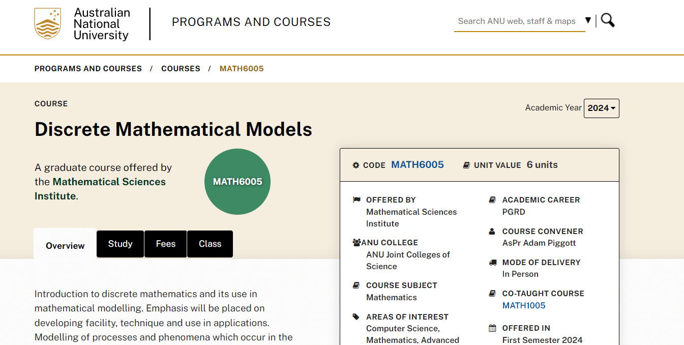
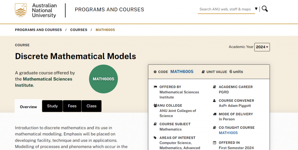
Course Code	MATH6005
Prerequisite Courses	Not explicitly mentioned in the provided text.
Majors	Mathematics
Teachers	AsPr Adam Piggott
Units	6 units

Discrete Mathematical Models离散数学模型问题集

问题 1.

Show by examples that neither the assertion in lemma 6.5 .2 nor Fermat’s “Little” Theorem remains valid if we drop the assumption that $p$ is a prime.
Consider a regular $p$-gon, and for a fixed $k(1 \leq k \leq p-1)$, consider all $k$-subsets of the set of its vertices. Put all these $k$-subsets into a number of boxes: We put two $k$-subsets into the same box if they can be rotated into each other. For example, all $k$-subsets consisting of $k$ consecutive vertices will belong to one and the same box.
(a) Prove that if $p$ is a prime, then each box will contain exactly $p$ of these rotated copies.
(b) Show by an example that (a) does not remain true if we drop the assumption that $p$ is a prime.
6.6 The Euclidean Algorithm
99
(c) Use (a) to give a new proof of Lemma

问题 2.

Imagine numbers written in base $a$, with at most $p$ digits. Put two numbers in the same box if they arike by a cyclic shift from each other. How many will be in each class? Give a new proof of Fermat’s Theorem this way.
Give a third proof of Fermat’s “Little” Theorem based on Exercise 6.3.5.
[Hint: Consider the product $a(2 a)(3 a) \cdots((p-1) a)$.]

问题 3.

Show that if $a$ and $b$ are positive integers with $a \mid b$, then $\operatorname{gcd}(a, b)=a$.
(a) Prove that $\operatorname{gcd}(a, b)=\operatorname{gcd}(a, b-a)$.
(b) Let $r$ be the remainder if we divide $b$ by $a$. Then $\operatorname{gcd}(a, b)=\operatorname{gcd}(a, r)$.

(a) If $a$ is even and $b$ is odd, then $\operatorname{gcd}(a, b)=\operatorname{gcd}(a / 2, b)$.
(b) If both $a$ and $b$ are even, then $\operatorname{gcd}(a, b)=2 \operatorname{gcd}(a / 2, b / 2)$.

How can you express the least common multiple of two integers if you know the prime factorization of each?

Suppose that you are given two integers, and you know the prime factorization of one of them. Describe a way of computing the greatest common divisor of these numbers.

Prove that for any two integers $a$ and $b$,
$$
\operatorname{gcd}(a, b) \operatorname{lcm}(a, b)=a b .
$$

澳洲代写｜MATH6005｜Discrete Mathematical Models离散数学模型澳洲国立大学

统计代写请认准statistics-lab™. statistics-lab™为您的留学生涯保驾护航。

金融工程代写

金融工程是使用数学技术来解决金融问题。金融工程使用计算机科学、统计学、经济学和应用数学领域的工具和知识来解决当前的金融问题，以及设计新的和创新的金融产品。

非参数统计代写

非参数统计指的是一种统计方法，其中不假设数据来自于由少数参数决定的规定模型；这种模型的例子包括正态分布模型和线性回归模型。

广义线性模型代考

广义线性模型（GLM）归属统计学领域，是一种应用灵活的线性回归模型。该模型允许因变量的偏差分布有除了正态分布之外的其它分布。

术语广义线性模型（GLM）通常是指给定连续和/或分类预测因素的连续响应变量的常规线性回归模型。它包括多元线性回归，以及方差分析和方差分析（仅含固定效应）。

有限元方法代写

有限元方法（FEM）是一种流行的方法，用于数值解决工程和数学建模中出现的微分方程。典型的问题领域包括结构分析、传热、流体流动、质量运输和电磁势等传统领域。

有限元是一种通用的数值方法，用于解决两个或三个空间变量的偏微分方程（即一些边界值问题）。为了解决一个问题，有限元将一个大系统细分为更小、更简单的部分，称为有限元。这是通过在空间维度上的特定空间离散化来实现的，它是通过构建对象的网格来实现的：用于求解的数值域，它有有限数量的点。边界值问题的有限元方法表述最终导致一个代数方程组。该方法在域上对未知函数进行逼近。[1] 然后将模拟这些有限元的简单方程组合成一个更大的方程系统，以模拟整个问题。然后，有限元通过变化微积分使相关的误差函数最小化来逼近一个解决方案。

tatistics-lab作为专业的留学生服务机构，多年来已为美国、英国、加拿大、澳洲等留学热门地的学生提供专业的学术服务，包括但不限于Essay代写，Assignment代写，Dissertation代写，Report代写，小组作业代写，Proposal代写，Paper代写，Presentation代写，计算机作业代写，论文修改和润色，网课代做，exam代考等等。写作范围涵盖高中，本科，研究生等海外留学全阶段，辐射金融，经济学，会计学，审计学，管理学等全球99%专业科目。写作团队既有专业英语母语作者，也有海外名校硕博留学生，每位写作老师都拥有过硬的语言能力，专业的学科背景和学术写作经验。我们承诺100%原创，100%专业，100%准时，100%满意。

随机分析代写

随机微积分是数学的一个分支，对随机过程进行操作。它允许为随机过程的积分定义一个关于随机过程的一致的积分理论。这个领域是由日本数学家伊藤清在第二次世界大战期间创建并开始的。

时间序列分析代写

随机过程，是依赖于参数的一组随机变量的全体，参数通常是时间。随机变量是随机现象的数量表现，其时间序列是一组按照时间发生先后顺序进行排列的数据点序列。通常一组时间序列的时间间隔为一恒定值（如1秒，5分钟，12小时，7天，1年），因此时间序列可以作为离散时间数据进行分析处理。研究时间序列数据的意义在于现实中，往往需要研究某个事物其随时间发展变化的规律。这就需要通过研究该事物过去发展的历史记录，以得到其自身发展的规律。

回归分析代写

多元回归分析渐进（Multiple Regression Analysis Asymptotics）属于计量经济学领域，主要是一种数学上的统计分析方法，可以分析复杂情况下各影响因素的数学关系，在自然科学、社会和经济学等多个领域内应用广泛。

MATLAB代写

MATLAB 是一种用于技术计算的高性能语言。它将计算、可视化和编程集成在一个易于使用的环境中，其中问题和解决方案以熟悉的数学符号表示。典型用途包括：数学和计算算法开发建模、仿真和原型制作数据分析、探索和可视化科学和工程图形应用程序开发，包括图形用户界面构建MATLAB 是一个交互式系统，其基本数据元素是一个不需要维度的数组。这使您可以解决许多技术计算问题，尤其是那些具有矩阵和向量公式的问题，而只需用 C 或 Fortran 等标量非交互式语言编写程序所需的时间的一小部分。MATLAB 名称代表矩阵实验室。MATLAB 最初的编写目的是提供对由 LINPACK 和 EISPACK 项目开发的矩阵软件的轻松访问，这两个项目共同代表了矩阵计算软件的最新技术。MATLAB 经过多年的发展，得到了许多用户的投入。在大学环境中，它是数学、工程和科学入门和高级课程的标准教学工具。在工业领域，MATLAB 是高效研究、开发和分析的首选工具。MATLAB 具有一系列称为工具箱的特定于应用程序的解决方案。对于大多数 MATLAB 用户来说非常重要，工具箱允许您学习和应用专业技术。工具箱是 MATLAB 函数（M 文件）的综合集合，可扩展 MATLAB 环境以解决特定类别的问题。可用工具箱的领域包括信号处理、控制系统、神经网络、模糊逻辑、小波、仿真等。

R语言代写	问卷设计与分析代写
PYTHON代写	回归分析与线性模型代写
MATLAB代写	方差分析与试验设计代写
STATA代写	机器学习/统计学习代写
SPSS代写	计量经济学代写
EVIEWS代写	时间序列分析代写
EXCEL代写	深度学习代写
SQL代写	各种数据建模与可视化代写

澳洲代写｜ECMT2130｜Financial Econometrics金融计量经济学悉尼大学

Posted on 2023年10月13日2023年10月13日 by statistics-lab

statistics-lab^TM为您悉尼大学（英语：The University of Sydney），简称悉大、USYD，简称“NCL”Financial Econometrics金融计量经济学澳洲代写代考和辅导服务！

课程介绍：

This unit focuses on the financial models and econometric methods necessary to critically evaluate the risk and return characteristics of various fund-management strategies. Asset-pricing models and market efficiency are tested using econometric models that are popular in banking and finance, using industry-standard software. A core learning outcome is competency with that software. Students work with real and simulated data to specify, estimate, and test the linear regression models and the univariate time-series models that are at the core of the unit. The unit equips students with the conceptual framework and applied skills relevant to quantitative careers in finance and policy.

澳洲代写｜ECMT2130｜Financial Econometrics金融计量经济学悉尼大学

Financial Econometrics金融计量经济学问题集

问题 1.

When the regressors in a multiple regression are highly correlated, then we have a practical problem: the standard errors of individual coefficients tend to be large.
As a simple example, consider the regression
$$
y_t=\beta_1 x_{1 t}+\beta_2 x_{2 t}+u_t
$$
where (for simplicity) the dependent variable and the regressors have zero means. In this case, the variance of
$$
\operatorname{Var}\left(\hat{\beta}2\right)=\frac{1}{1-\operatorname{Corr}\left(x{1 t}, x_{2 t}\right)^2} \frac{1}{\operatorname{Var}\left(x_{2 t}\right)} \frac{\sigma^2}{T},
$$
where the new term is the (squared) correlation. If the regressors are highly correlated, then the uncertainty about the slope coefficient is high. The basic reason is that we see that the variables have an effect on $y_t$, but it is hard to tell if that effect is from regressor one or two.

Proof. (of 2.21). Recall that for a $2 \times 2$ matrix we have
$$
\left[\begin{array}{ll}
a & b \
c & d
\end{array}\right]^{-1}=\frac{1}{a d-b c}\left[\begin{array}{cc}
d & -b \
-c & a
\end{array}\right] .
$$
For the regression (2.20) we get
$$
\begin{aligned}
& {\left[\begin{array}{cc}
\sum_{t=1}^T x_{1 t}^2 & \sum_{t=1}^T x_{1 t} x_{2 t} \
\sum_{t=1}^T x_{1 t} x_{2 t} & \sum_{t=1}^T x_{2 t}^2
\end{array}\right]^{-1}=} \
& \quad \frac{1}{\sum_{t=1}^T x_{1 t}^2 \sum_{t=1}^T x_{2 t}^2-\left(\sum_{t=1}^T x_{1 t} x_{2 t}\right)^2}\left[\begin{array}{cc}
\sum_{t=1}^T x_{2 t}^2 & -\sum_{t=1}^T x_{1 t} x_{2 t} \
-\sum_{t=1}^T x_{1 t} x_{2 t} & \sum_{t=1}^T x_{1 t}^2
\end{array}\right] .
\end{aligned}
$$
The variance of the second slope coefficient is $\sigma^2$ time the lower right element of this

matrix. Multiply and divide by $T$ to get
$$
\begin{aligned}
\operatorname{Var}\left(\hat{\beta}2\right) & =\frac{\sigma^2}{T} \frac{\sum{t=1}^T x_{1 t}^2 / T}{\sum_{t=1}^T \frac{1}{T} x_{1 t}^2 \sum_{t=1}^T \frac{1}{T} x_{2 t}^2-\left(\sum_{t=1}^T \frac{1}{T} x_{1 t} x_{2 t}\right)^2} \
& =\frac{\sigma^2}{T} \frac{\operatorname{Var}\left(x_{1 t}\right)}{\operatorname{Var}\left(x_{1 t}\right) \operatorname{Var}\left(x_{2 t}\right)-\operatorname{Cov}\left(x_{1 t}, x_{2 t}\right)^2} \
& =\frac{\sigma^2}{T} \frac{1 / \operatorname{Var}\left(x_{2 t}\right)}{1-\frac{\operatorname{Cov}\left(x_{1 t}, x_{2 t}\right)^2}{\operatorname{Var}\left(x_{1 t}\right) \operatorname{Var}\left(x_{2 t}\right)}}
\end{aligned}
$$

问题 2.

Suppose we have monthly data with $\widehat{\alpha}i=0.2 \%$ (that is, $0.2 \% \times 12=2.4 \%$ per year), Std $\left(\varepsilon{i t}\right)=3 \%$ (that is, $3 \% \times \sqrt{12} \approx 10 \%$ per year) and a market Sharpe ratio of 0.15 (that is, $0.15 \times \sqrt{12} \approx 0.5$ per year). (This corresponds well to US CAPM regressions for industry portfolios.) A significance level of $10 \%$ requires a $t$-statistic (6.4) of at least 1.65 , so
$$
\frac{0.2}{\sqrt{1+0.15^2} 3 / \sqrt{T}} \geq 1.65 \text { or } T \geq 626 .
$$
We need a sample of at least 626 months (52 years)! With a sample of only 26 years (312 months), the alpha needs to be almost $0.3 \%$ per month (3.6\% per year) or the standard deviation of the residual just $2 \%$ (7\% per year). Notice that cumulating a $0.3 \%$ return over 25 years means almost 2.5 times the initial value.

Proof. (*Proof of (6.8)) Consider the regression equation $y_t=x_t^{\prime} b+\varepsilon_t$. With iid errors that are independent of all regressors (also across observations), the LS estimator, $\hat{b}{L s}$, is asymptotically distributed as $$ \sqrt{T}\left(\hat{b}{L s}-b\right) \stackrel{d}{\rightarrow} N\left(\mathbf{0}, \sigma^2 \Sigma_{x x}^{-1}\right) \text {, where } \sigma^2=\operatorname{Var}\left(\varepsilon_t\right) \text { and } \Sigma_{x x}=\operatorname{plim} \Sigma_{t=1}^T x_t x_t^{\prime} / T .
$$
When the regressors are just a constant (equal to one) and one variable regressor, $f_t$, so $x_t=\left[1, f_t\right]^{\prime}$, then we have
$$
\begin{aligned}
\Sigma_{x x} & =\mathrm{E} \sum_{t=1}^T x_t x_t^{\prime} / T=\mathrm{E} \frac{1}{T} \sum_{t=1}^T\left[\begin{array}{cc}
1 & f_t \
f_t & f_t^2
\end{array}\right]=\left[\begin{array}{cc}
1 & \mathrm{E} f_t \
\mathrm{E} f_t & \mathrm{E} f_t^2
\end{array}\right], \text { so } \
\sigma^2 \Sigma_{x x}^{-1} & =\frac{\sigma^2}{\mathrm{E} f_t^2-\left(\mathrm{E} f_t\right)^2}\left[\begin{array}{cc}
\mathrm{E} f_t^2 & -\mathrm{E} f_t \
-\mathrm{E} f_t & 1
\end{array}\right]=\frac{\sigma^2}{\operatorname{Var}\left(f_t\right)}\left[\begin{array}{cc}
\operatorname{Var}\left(f_t\right)+\left(\mathrm{E} f_t\right)^2 & -\mathrm{E} f_t \
-\mathrm{E} f_t & 1
\end{array}\right] .
\end{aligned}
$$
(In the last line we use $\operatorname{Var}\left(f_t\right)=\mathrm{E} f_t^2-\left(\mathrm{E} f_t\right)^2$.)

问题 3.

It is then straightfoward to show that the VaR for a portfortfolio
$$
R_p=w_1 R_1+w_2 R_2,
$$

where $w_1+w_2=1$ can be written
$$
\operatorname{VaR}p=\left(\left[\begin{array}{ll} w_1 \operatorname{Var}_1 & w_2 \operatorname{Var}_2 \end{array}\right]\left[\begin{array}{cc} 1 & \rho{12} \
\rho_{12} & 1
\end{array}\right]\left[\begin{array}{l}
w_1 \operatorname{Var}1 \ w_2 \operatorname{Var}_2 \end{array}\right]\right)^{1 / 2}, $$ where $\rho{12}$ is the correlation of $R_1$ and $R_2$. The extension to $n$ (instead of 2) assets is straightforward.

This expression highlights the importance of both the individual $\mathrm{VaR}i$ values and the correlation. Clearly, a worst case scenario is when the portfolio is long in all assets $\left(w_i>\right.$ $0)$ and the correlation turns out to be perfect $\left(\rho{12}=1\right)$.

Proof. (of (11.8)) Recall that $\mathrm{VaR}p=1.64 \sigma_p$, and that $$ \sigma_p^2=w_1^2 \sigma{11}+w_2^2 \sigma_{22}+2 w_1 w_2 \rho_{12} \sigma_1 \sigma_2
$$
Use (11.6) to substitute as $\sigma_i=\operatorname{VaR}i / 1.64$ $$ \sigma_p^2=w_1^2 \operatorname{VaR}_1^2 / 1.64^2+w_2^2 \operatorname{VaR}_2^2 / 1.64^2+2 w_1 w_2 \rho{12} \times \operatorname{VaR}_1 \times \mathrm{VaR}_2 / 1.64^2 .
$$
Multiply both sides by $1.64^2$ and take the square root to get (11.8).

统计代写请认准statistics-lab™. statistics-lab™为您的留学生涯保驾护航。

金融工程代写

非参数统计代写

非参数统计指的是一种统计方法，其中不假设数据来自于由少数参数决定的规定模型；这种模型的例子包括正态分布模型和线性回归模型。

广义线性模型代考

广义线性模型（GLM）归属统计学领域，是一种应用灵活的线性回归模型。该模型允许因变量的偏差分布有除了正态分布之外的其它分布。

有限元方法代写

随机分析代写

时间序列分析代写

回归分析代写

MATLAB代写

R语言代写	问卷设计与分析代写
PYTHON代写	回归分析与线性模型代写
MATLAB代写	方差分析与试验设计代写
STATA代写	机器学习/统计学习代写
SPSS代写	计量经济学代写
EVIEWS代写	时间序列分析代写
EXCEL代写	深度学习代写
SQL代写	各种数据建模与可视化代写

澳洲代写｜ENVX2001｜Applied Statistical Method应用统计方法悉尼大学

Posted on 2023年10月13日2023年10月13日 by statistics-lab

statistics-lab^TM为您悉尼大学（英语：The University of Sydney），简称悉大、USYD，简称“NCL”Applied Statistical Method应用统计方法代写代考和辅导服务！

课程介绍：

This unit builds on introductory 1st year statistics units and is targeted towards students in the agricultural, life and environmental sciences. It consists of two parts and presents, in an applied manner, the statistical methods that students need to know for further study and their future careers. In the first part the focus is on designed studies including both surveys and formal experimental designs. Students will learn how to analyse and interpret datasets collected from designs from more than 2 treatment levels, multiple factors and different blocking designs. In the second part the focus is on finding patterns in data. In this part the students will learn to model relationships between response and predictor variables using regression, and find patterns in datasets with many variables using principal components analysis and clustering. This part provides the foundation for the analysis of big data. In the practicals the emphasis is on applying theory to analysing real datasets using the statistical software package R. A key feature of the unit is using R to develop coding skills that have become essential in science for processing and analysing datasets of ever-increasing size.

澳洲代写｜ENVX2001｜Applied Statistical Method应用统计方法悉尼大学

Detail	Information
Unit Code	ENVX2001
Unit Name	Applied Statistical Methods
Academic Unit	Life and Environmental Sciences Academic Operations
Session, Year	Semester 1, 2023
Location	Camperdown/Darlington, Sydney
Credit Points	6

Applied Statistical Method应用统计方法问题集

问题 1.

Consider the following set of numbers: $2,5,6,7,11,15,20,22$, and 23 . Find the sum of the first 3 numbers.

Solution:
This set of numbers forms an array, since they are listed in order from the smallest to the largest. To sum the first three numbers we write
$$
\sum_{i=1}^3 X_i=X_1+X_2+X_3=2+5+6=13 .
$$
The expression $i=1$, below the summation sign, is called the lower limit of the summation, and the number 3 , in this case, is called the upper limit. In general, in case we like to add all the numbers in the array, the order here does not matter. We can add them in any order they are given. There is no need to arrange them in an array.

问题 2.

Consider the $\mathrm{X}$ array as $2,4,6$, and 8 ; while the $\mathrm{Y}$ array to be given by $3,5,7$, and 9 .

$$
\begin{aligned}
& \sum_{i=1}^4 X_i Y_i=2(3)+4(5)+6(7)+8(9)=6+20+42+72=140 \
& \left(\sum_{i=1}^4 X_i\right) \cdot\left(\sum_{i=1}^4 Y_i\right)=(2+4+6+8) \cdot(3+5+7+9)=20 \cdot 24=480 .
\end{aligned}
$$
No doubt, we see that $140 \neq 480$.

问题 3.

Consider the following set of data: $5,8,12,15$, and 20. For this data, find
a) The geometric mean,
b) The harmonic mean.
c) Compare the above three means: $\bar{x}, \bar{G}$, and $\bar{H}$.

a) The geometric mean is given by $\bar{G}=\left(x_1, x_2 \ldots x_n\right)^{1 / n}$, and we have $n=5$, and $X_1=5, X_2=8$, $\mathrm{X}_3=12, \mathrm{X}_4=15$, and $\mathrm{X}_5=20$. Applying the formula for, $\bar{G}$ we see that with a graphing calculator that $\bar{G}=\left(5^{\star} 8^{\star} 12^{\star} 15^{\star} 20\right)^{1 / 5}=(144000)^{1 / 5}=10.7565$.
b) The Harmonic mean is given by $\bar{H}=n / \sum_1^n\left(1 / X_i\right)$. From the data, and by using a graphing calculator we find that $\bar{H}=5 /[1 / 5+1 / 8+1 / 12+1 / 15+1 / 20]=9.524$.
c) For the comparison, we need to calculate the arithmetic mean $\bar{x}$. It is easily found that it equals to $60 / 5=12$. Therefore we have $\bar{H}<\bar{G}<\bar{x}$.

统计代写请认准statistics-lab™. statistics-lab™为您的留学生涯保驾护航。

金融工程代写

非参数统计代写

非参数统计指的是一种统计方法，其中不假设数据来自于由少数参数决定的规定模型；这种模型的例子包括正态分布模型和线性回归模型。

广义线性模型代考

广义线性模型（GLM）归属统计学领域，是一种应用灵活的线性回归模型。该模型允许因变量的偏差分布有除了正态分布之外的其它分布。

有限元方法代写

随机分析代写

时间序列分析代写

回归分析代写

MATLAB代写

R语言代写	问卷设计与分析代写
PYTHON代写	回归分析与线性模型代写
MATLAB代写	方差分析与试验设计代写
STATA代写	机器学习/统计学习代写
SPSS代写	计量经济学代写
EVIEWS代写	时间序列分析代写
EXCEL代写	深度学习代写
SQL代写	各种数据建模与可视化代写

澳洲代写｜ECOS3007｜ International Macroeconomics国际宏观经济学悉尼大学

Posted on 2023年10月13日2023年10月13日 by statistics-lab

statistics-lab^TM为您悉尼大学（英语：The University of Sydney），简称悉大、USYD，简称“NCL”Stochastic Processes随机过程代写代考和辅导服务！

课程介绍：

This unit studies macroeconomic theory and policy in a global trading world. The microfoundations of the various sectors are examined in the context of an open economy. The evolution of international money and capital markets is described, the operation of the foreign exchange market is examined, showing how its microstructure affects its macro performance. Theories and tests of the efficiency of international capital markets are surveyed, as well as core theories and tests of exchange rate and asset price determination. The unit develops the macroeconomic implications of monetary and fiscal policies for small and large open economies for different regimes.

澳洲代写｜ECOS3007｜ International Macroeconomics国际宏观经济学悉尼大学

Attribute	Detail
Course Code	ECOS3007
Course Title	International Macroeconomics
Academic Unit	Economics
Session, Year	Semester 1, 2023
Location	Camperdown/Darlington, Sydney
Credit Points	6
Coordinator/Lecturer	Not Specified
Pre-Requisites	Not Specified

International Macroeconomics国际宏观经济学相关

Assume that there exists free international capital mobility and that the world interest rate, $r^$, is $10 \%$ per period (i.e., $r^=0.1$ ). Finally,

assume that the economy’s initial net foreign asset position is zero $\left(B_0^*=0\right)$.
(a) Compute the firm’s optimal levels of period-1 investment and period-2 profits.
(b) State the maximization problem of the representative household and solve for the optimal levels of consumption in periods 1 and 2.
(c) Find the country’s net foreign asset position at the end of period 1 , the trade balance in periods 1 and 2 , and the current account in periods 1 and 2 .
(d) Now consider an investment surge. Specifically, assume that as a result of a technological improvement, the production technology becomes $Q_2=2 \sqrt{T_1}$. Find the equilibrium levels of savings, investment, the trade balance, the current account, and the country’s net foreign asset position in period 1. Compare your results with those obtained in items (a)-(c) providing interpretation and intuition.

假设存在自由的国际资本流动性，并且世界利率 $r^$ 为每期 $10 \%$ （即 $r^=0.1$ ）。最后，

假设经济体的初始净外国资产头寸为零$\left(B_0^*=0\right)$。
(a) 计算公司第一期投资和第二期利润的最佳水平。
(b) 陈述代表性家庭的最大化问题并求解第 1 期和第 2 期的最优消费水平。
(c) 求该国在第 1 期末的外国净资产头寸、第 1 期和第 2 期的贸易差额以及第 1 期和第 2 期的经常账户。
(d) 现在考虑投资激增。具体来说，假设由于技术改进，生产技术变为$Q_2=2 \sqrt{T_1}$。求第 1 期储蓄、投资、贸易平衡、经常账户和国家净外国资产头寸的均衡水平。将您的结果与 (a)-(c) 项中获得的结果进行比较，以提供解释和直觉。

An investment surge
Suppose that in period 1 agents learn that in period 2 the productivity of capital will increase. For example, suppose that the production function in period 2 was initially given by $F\left(K_2\right)=\sqrt{K_2}$ and that due to a technological advancement it changes to $\tilde{F}\left(K_2\right)=2 \sqrt{K_2}$. Another example of an investment surge is given by an expected increase in the price of exports. In Norway, for instance, the oil price increase of 1973 unleashed an investment boom of around $10 \%$ of GDP. In response to this news, firms will choose to increase investment in period 1 for any given level of the interest rate. This scenario is illustrated in figure 6.4. Initially, the investment schedule is $I^0\left(r_1\right)$ and the saving schedule is $S^0\left(r_1, Q_1\right)$. Given the world interest rate $r^*$, investment is $I_1^0$ and savings is $S_1^0$. As shown in panel (b), the current account schedule is $C A^0\left(r_1, Q_1\right)$, and the equilibrium current account balance is $C A_1^0$. The news of the future productivity increase shifts the investment schedule to the right to $I^1\left(r_1\right)$, and the new equilibrium level of investment is $I_1^1$, which is higher than $I_1^0$. The expected increase in productivity might also affect current saving through its effect on expected future income. Specifically, in period 2, firms will generate higher profits which represent a positive income effect for households who are the owners of such firms. Households will take advantage of the expected increase in profits by increasing consumption in period 1 , thus cutting savings. Therefore, the savings schedule shifts to the left to $S^1\left(r_1, Q_1\right)$ and the equilibrium level of savings falls from $S_1^0$ to $S_1^1$. With this shifts in the investment and savings schedules it follows that, for any given interest rate, the current account is lower. That is, the current account schedule shifts to the left to $C A^1\left(r_1, Q_1\right)$. Given the world interest rate $r^*$, the current account deteriorates from $C A_1^0$ to $C A_1^1$. Note that if the economy was closed, the investment surge would trigger a rise in the domestic interest rate from $r_c^0$ to $r_c^1$ and thus investment would increase by less than in the open economy.

投资激增
假设在第 1 阶段，代理人得知在第 2 阶段，资本生产率将会提高。例如，假设第 2 期的生产函数最初由 $F\left(K_2\right)=\sqrt{K_2}$ 给出，并且由于技术进步，它变为 $\tilde{F}\left( K_2\right)=2\sqrt{K_2}$。投资激增的另一个例子是出口价格的预期上涨。例如，在挪威，1973 年石油价格上涨引发了投资热潮，投资额约占 GDP 的 10%$。针对这一消息，企业将选择在任何给定利率水平下增加第一阶段的投资。这种情况如图 6.4 所示。最初，投资计划为 $I^0\left(r_1\right)$，储蓄计划为 $S^0\left(r_1, Q_1\right)$。给定世界利率 $r^$，投资为 $I_1^0$，储蓄为 $S_1^0$。如图(b)所示，经常账户表为$C A^0\left(r_1, Q_1\right)$，平衡经常账户余额为$C A_1^0$。未来生产率提高的消息使投资计划右移为$I^1\left(r_1\right)$，新的投资均衡水平为$I_1^1$，高于$I_1^0 $。生产率的预期增长也可能通过对预期未来收入的影响而影响当前储蓄。具体来说，在第二阶段，企业将产生更高的利润，这对这些企业所有者的家庭产生积极的收入影响。家庭将通过增加第一阶段的消费来利用预期的利润增长，从而减少储蓄。因此，储蓄计划向左移动到$S^1\left(r_1, Q_1\right)$，储蓄均衡水平从$S_1^0$下降到$S_1^1$。随着投资和储蓄计划的这种变化，对于任何给定的利率，经常账户都会较低。即当前账户表左移为$C A^1\left(r_1, Q_1\right)$。考虑到世界利率 $r^$，经常账户从 $C A_1^0$ 恶化到 $C A_1^1$。请注意，如果经济封闭，投资激增将引发国内利率从 $r_c^0$ 上升至 $r_c^1$，因此投资增幅将低于开放经济。

统计代写请认准statistics-lab™. statistics-lab™为您的留学生涯保驾护航。

金融工程代写

非参数统计代写

非参数统计指的是一种统计方法，其中不假设数据来自于由少数参数决定的规定模型；这种模型的例子包括正态分布模型和线性回归模型。

广义线性模型代考

广义线性模型（GLM）归属统计学领域，是一种应用灵活的线性回归模型。该模型允许因变量的偏差分布有除了正态分布之外的其它分布。

有限元方法代写

随机分析代写

时间序列分析代写

回归分析代写

MATLAB代写

R语言代写	问卷设计与分析代写
PYTHON代写	回归分析与线性模型代写
MATLAB代写	方差分析与试验设计代写
STATA代写	机器学习/统计学习代写
SPSS代写	计量经济学代写
EVIEWS代写	时间序列分析代写
EXCEL代写	深度学习代写
SQL代写	各种数据建模与可视化代写

澳洲代写｜MATH1510｜Stochastic Processes随机过程悉尼大学

Posted on 2023年10月13日2023年10月13日 by statistics-lab

statistics-lab^TM为您悉尼大学（英语：The University of Sydney），简称悉大、USYD，简称“NCL”Stochastic Processes随机过程代写代考和辅导服务！

课程介绍：

A stochastic process is a mathematical model of time-dependent random phenomena and is employed in numerous fields of application, including economics, finance, insurance, physics, biology, chemistry and computer science. This unit will establish basic properties of discrete-time Markov chains including random walks and branching processes. This unit will derive key results of Poisson processes and simple continuous-time Markov chains. This unit will investigate simple queuing theory. This unit will also introduce basic concepts of Brownian motion and martingales. Throughout the unit, various illustrative examples are provided in modelling and analysing problems of practical interest. By completing this unit, you will develop an essential basis for further studies stochastic analysis, stochastic differential equations, stochastic control, financial mathematics and statistical inference.

澳洲代写｜MATH1510｜Stochastic Processes随机过程悉尼大学

Attribute	Detail
Course Code	STAT3021
Course Title	Stochastic Processes
Academic Unit	Mathematics and Statistics Academic Operations
Session, Year	Semester 1, 2023
Location	Camperdown/Darlington, Sydney
Credit Points	6
Coordinator/Lecturer	Not Specified
Pre-Requisites	Not Specified

Stochastic Processes随机过程代写代考作业问题集

问题 1.

Consider the unit interval $I:=[0,1]$. Moreover, for every $n$ and $\left(i_1, \ldots, i_n\right) \in{0,1,2}^n$ we consider the interval $I_{i_1 \ldots i_n} \subset I$ which is the set of those numbers whose base 3 expansion starts with $\left(i_1 \ldots i_n\right)$. That is
$$
I_{i_1 \ldots i_n}:=\left[\sum_{k=1}^n \frac{i_k}{3^k}, \frac{1}{3^n}+\sum_{k=1}^n \frac{i_k}{3^k}\right] .
$$
Let $X_0, X_1, X_2$ be independent $\operatorname{Bernoulli}\left(p_0\right)$, Bernoulli $\left(p_1\right)$ and $\operatorname{Bernoulli}\left(p_2\right)$ random variables respectively. That is $\mathbb{P}\left(X_i=1\right)=p_i$ and $\mathbb{P}\left(X_i=0\right)=1-p_i$ for $i=0,1,2$. Moreover for every $n$ and $\left(i_1, \ldots, i_n\right) \in{0,1,2}^n$ we are given the random variables $X_{i_1 \ldots i_n}$ such that on the one hand $\left{X_{i_1 \ldots i_n}\right}_{n \geq 1,\left(i_1, \ldots, i_n\right) \in{0,1,2}^n}$ are independent and on the other hand: $X_{i_1 \ldots i_n} \stackrel{d}{=} X_{i_n}$. For every $n \geq 1$ we define the set $E_n \subset[0,1]$ by
$$
E_n:=\bigcup_{X_{i_1} \cdot X_{i_1, i_2} \cdots X_{i_1, i_2, \ldots, i_n}=1} I_{i_1 \ldots i_n} .
$$
Finally, we define the set $E:=\bigcap_{n=1}^{\infty} E_n$. Assume that $p_0=\frac{2}{3}, p_1=\frac{3}{4}$ and $p_2=\frac{1}{2}$. Question: Is it true that $\mathbb{P}(E \neq \emptyset)>0$

问题 2.

Given a branching process with the following offspring distribution, determine the extinction probabilities $q$ :
(a) $p_0=0.25, p_1=0.4, p_2=0.35, p_n=0$ if $n \geq 3$,
(b) $p_0=0.5, p_1=0.1, p_2=0, p_3=0.4, p_n=0$ if $n \geq 4$

问题 3.

Consider the branching process with offspring distribution as in the previous exercise part (b). What is the probability that the population is extinct in the second generation $X_2=0$, given that it did not die out in the first generation?

英国代写｜MATH1510｜Discrete Mathematics离散数学悉尼大学

统计代写请认准statistics-lab™. statistics-lab™为您的留学生涯保驾护航。

金融工程代写

非参数统计代写

非参数统计指的是一种统计方法，其中不假设数据来自于由少数参数决定的规定模型；这种模型的例子包括正态分布模型和线性回归模型。

广义线性模型代考

广义线性模型（GLM）归属统计学领域，是一种应用灵活的线性回归模型。该模型允许因变量的偏差分布有除了正态分布之外的其它分布。

有限元方法代写

随机分析代写

时间序列分析代写

回归分析代写

MATLAB代写

R语言代写	问卷设计与分析代写
PYTHON代写	回归分析与线性模型代写
MATLAB代写	方差分析与试验设计代写
STATA代写	机器学习/统计学习代写
SPSS代写	计量经济学代写
EVIEWS代写	时间序列分析代写
EXCEL代写	深度学习代写
SQL代写	各种数据建模与可视化代写

英国代写｜MATH1510｜Discrete Mathematics离散数学纽卡斯尔大学

Posted on 2023年10月12日2023年10月13日 by statistics-lab

statistics-lab^TM为您纽卡斯尔大学（Newcastle University），简称“NCL”Discrete Mathematics离散数学英国代写代考和辅导服务！

课程介绍：

Discrete mathematics is the study of mathematical structures that are discrete, separated or distinct; in contrast with calculus which deals with continuous change. It is an important area of pure and applied mathematics, as well as providing the mathematical basis for the understanding of computers and modern computation. Discrete Mathematics is important in the sciences, where it has increasing application in many areas, an exemplar of which is the understanding of DNA sequences in molecular biology. The Discrete Mathematics course introduces first year students to the basic concepts of discrete mathematics, covering topics such as sets, logic, enumeration methods, probability, recurrence relations, induction and graph theory. The course provides important background for students pursuing a BMath degree. It covers much of the mathematics essential for students majoring in Computer Science or Software Engineering, and is a compulsory course in those degree programs.

Attribute	Detail
Course Code	MATH1510
Course Title	Discrete Mathematics
Units	10 units
Level	1000 level
Pre-Requisites	HSC Advanced Mathematics (Bands 5 or 6), or equivalent
Course Coordinator/Lecturer	Not explicitly mentioned in the provided text

Discrete Mathematics离散数学的案例

问题 1.

Let $\phi: G \rightarrow H$ be a group isomorphism. If $g \in G$ then the group inverse, in the group $H$, of $\phi(g)$ is $\phi\left(g^{-1}\right)$.

Proof: We may check that
$$
\phi(g) \cdot \phi\left(g^{-1}\right)=\phi\left(g \cdot g^{-1}\right)=\phi\left(e_G\right)=e_H
$$
(by Proposition 9.5)
Also
$$
\phi\left(g^{-1}\right) \cdot \phi(g)=\phi\left(g^{-1} \cdot g\right)=\phi\left(e_G\right)=e_H
$$
(by Proposition 9.5)
Thus $\phi\left(g^{-1}\right)$ possesses the defining properties of the group inverse of $\phi(g)$. Since the group inverse of any group element is unique, our result follows.

The theory of groups has become a large and essential part of modern mathematics. It is also used in physics (in quantum mechanics, for instance), in engineering, and in theoretical computer science (for example, data compression theory uses group theory).

It is a classical result of basic group theory that all finite abelian groups have been classified. Indeed, it can be shown that any such group is a product (in the sense of set theory) of cyclic groups. One of the triumphs of twentieth century mathematics is that all groups of finite order have been classified. This result is the product of the work of hundreds of mathematicians and will ultimately produce a book of several thousand pages.

问题 2.

If $n$ is a positive integer and $k$ is relatively prime to $n$ then
$$
k^{\varphi(n)}=1 \bmod n
$$

Proof: The proof of this result is easy. For the collection $\mathcal{P}(n)$ of numbers relatively prime to $n$ forms a group under multiplication. That is, if $a$ is relatively prime to $n$ and $b$ is relatively prime to $n$ then logic dictates that $a \cdot b$ is relatively prime to $n$. Now it is a fundamental fact-we cannot prove it here, but see [BMS] – that if a group has $m$ elements and $g$ is an element of the group then $g^m$ is the group identity. Thus any element of the group, raised to the power $\varphi(n)$ (the number of elements in the group) will equal 1 modulo $n$.

For later use, it is worth noting that if $p, q$ are prime numbers and $n=p \cdot q$ then $\varphi(n)=(p-1) \cdot(q-1)$.

The reason is that the only numbers less than or equal to $n$ that are not relatively prime to $n$ are $p, 2 p, 3 p, \ldots q \cdot p$ and $q, 2 q, 3 q, \cdots(p-1) q$.

There are $q$ numbers in the first list and $p-1$ numbers in the second list. The set $\mathcal{P}(n)$ of numbers relatively prime to $n$ is the complement of these two lists, and it therefore has
$$
p q-q-(p-1)=p q-q-p+1=(p-1) \cdot(q-1) \equiv \varphi(n)
$$
elements.

问题 3.

A quantity of radioactive material decays. At the beginning of each week there is half as much as there was the previous week. The initial quantity is 5 grams. Use sequence notation to express the amount of material at the beginning of the $j$ th week.

Solution: The amount of radioactive material at the beginning of the second week is $5 / 2$ (half as much as the initial amount at the beginning of the first week). The amount at the beginning of the third week is 5/4. The amount at the beginning of the fourth week is $5 / 8$. And so forth.

As a result, according to the description, the amount of material at the start of the $j$ th week is
$$
a_j=5 \cdot\left(\frac{1}{2}\right)^{j-1}
$$
The sequence exhibits in an elegant way the process of radioactive decay: the first several values are
$$
5, \frac{5}{2}, \frac{5}{4}, \frac{5}{8}
$$
It is easy to see intuitively, or with a calculator, that the amount of radioactive material tends to 0 as time tends to $\infty$.

统计代写请认准statistics-lab™. statistics-lab™为您的留学生涯保驾护航。

金融工程代写

非参数统计代写

非参数统计指的是一种统计方法，其中不假设数据来自于由少数参数决定的规定模型；这种模型的例子包括正态分布模型和线性回归模型。

广义线性模型代考

广义线性模型（GLM）归属统计学领域，是一种应用灵活的线性回归模型。该模型允许因变量的偏差分布有除了正态分布之外的其它分布。

有限元方法代写

随机分析代写

时间序列分析代写

回归分析代写

MATLAB代写

R语言代写	问卷设计与分析代写
PYTHON代写	回归分析与线性模型代写
MATLAB代写	方差分析与试验设计代写
STATA代写	机器学习/统计学习代写
SPSS代写	计量经济学代写
EVIEWS代写	时间序列分析代写
EXCEL代写	深度学习代写
SQL代写	各种数据建模与可视化代写

STAT0013｜Discrete Mathematics 离散数学伦敦大学学院

Posted on 2023年9月22日2023年10月6日 by statistics-lab

statistics-lab^TM为您提供伦敦大学学院 London’s Global University STAT0013 Mathematical Analysis数学分析英国代写代考和辅导服务！

课程介绍：

STAT0013 is specified as a formal option for third and fourth year undergraduates from the Department of Mathematics. Any such student who has taken one of the standard prerequisites (simultaneous attendance of STAT0005 is also acceptable) should simply register for STAT0013 on Portico and await a decision. Mathematics students who do not satisfy the standard prerequisites must additionally consult a member of staff in the Department of Statistical Science.

STAT0013｜Discrete Mathematics (Advanced)进阶离散数学伦敦大学学院

Discrete Mathematics 离散数学作业案例

问题 1.

Let
$$
B=\left(\begin{array}{rrr}
-7 & 4 & -3 \
2 & -5 & 3 \
1 & -3 & -2
\end{array}\right)
$$
Calculate det $B$.

Solution: We calculate that
$$
\begin{aligned}
\operatorname{det} B= & (-7) \cdot \operatorname{det}\left(\begin{array}{rr}
-5 & 3 \
-3 & -2
\end{array}\right) \
& -4 \cdot \operatorname{det}\left(\begin{array}{rr}
2 & 3 \
1 & -2
\end{array}\right) \
& +(-3) \cdot \operatorname{det}\left(\begin{array}{rr}
2 & -5 \
1 & -3
\end{array}\right) \
= & (-7) \cdot 19-4 \cdot(-7)+(-3) \cdot(-1) \
= & -102 \
\neq & 0 .
\end{aligned}
$$
It is worth summarizing the main rule for inverses for which we have given an indication of the justification:

Rule for inverses: A square matrix has an inverse if and only if the matrix has nonzero determinant.

This still does not tell us how to find the inverse, but we shall get to that momentarily.
There are in fact a number of ways to calculate the inverse of a matrix, and we shall indicate two of them here. The first is the method of Gaussian elimination, which is a powerful technique that can be used for many purposes. The idea is to take the given square matrix
$$
A=\left(\begin{array}{ll}
a & b \
c & d
\end{array}\right)
$$
and to augment it by adjoining the identity matrix as in the display below:
$$
\left(\begin{array}{ll|ll}
a & b & 1 & 0 \
c & d & 0 & 1
\end{array}\right)
$$
Now the method of gaussian elimination allows us to perform certain operations on the rows of this augmented matrix, the goal being to reduce the square matrix on the left to the identity matrix. Whatever matrix results on the right will be the inverse.

问题 2.

The multiplicative identity for a group is unique.

Proof: Let $G$ be a group. Let $e$ and $e^{\prime}$ both be elements of $G$ that satisfy Axiom 2 . Then
$$
e=e \cdot e^{\prime}=e^{\prime}
$$
Thus $e$ and $e^{\prime}$ must be the same group element.

STAT0013｜Discrete Mathematics 离散数学伦敦大学学院

统计代写请认准statistics-lab™. statistics-lab™为您的留学生涯保驾护航。

金融工程代写

非参数统计代写

非参数统计指的是一种统计方法，其中不假设数据来自于由少数参数决定的规定模型；这种模型的例子包括正态分布模型和线性回归模型。

广义线性模型代考

广义线性模型（GLM）归属统计学领域，是一种应用灵活的线性回归模型。该模型允许因变量的偏差分布有除了正态分布之外的其它分布。

有限元方法代写

随机分析代写

时间序列分析代写

回归分析代写

MATLAB代写

R语言代写	问卷设计与分析代写
PYTHON代写	回归分析与线性模型代写
MATLAB代写	方差分析与试验设计代写
STATA代写	机器学习/统计学习代写
SPSS代写	计量经济学代写
EVIEWS代写	时间序列分析代写
EXCEL代写	深度学习代写
SQL代写	各种数据建模与可视化代写

Math1904｜Discrete Mathematics (Advanced)进阶离散数学悉尼大学

Posted on 2023年9月22日2023年10月6日 by statistics-lab

statistics-lab^TM为您提供悉尼大学University of Sydney Math1904 Mathematical Analysis数学分析澳洲代写代考和辅导服务！

课程介绍：

This unit of study provides an introduction to programming and numerical methods. Topics covered include computer arithmetic and computational errors, systems of linear equations, interpolation and approximation, solution of nonlinear equations, quadrature, initial value problems for ordinary differential equations and boundary value problems, and optimisation.

Math1904｜Discrete Mathematics (Advanced)进阶离散数学悉尼大学

Discrete Mathematics (Advanced)进阶离散数学作业案例

问题 1.

Let $g:[1,+\infty) \rightarrow[8,+\infty)$ be given by $g(x)=x^2+3 x+4$. Then $g(1)=8$, and $g$ is strictly increasing without bound. So $g$ is one-to-one and onto. We conclude that $g$ has an inverse. One may use the quadratic formula to solve for that inverse, and find that $g^{-1}(x)=(-3+\sqrt{-7+4 x}) / 2$.

The idea of inverse function lends itself particularly well to the notation of ordered pairs. For $f: S \rightarrow T$ is inverse to $g: T \rightarrow S$ (and vice versa) provided that for every ordered pair $(s, t) \in f$ there is an ordered pair $(t, s) \in g$ and conversely.
Not every function has an inverse. For instance, let $f: S \rightarrow T$. Suppose that $f(s)=t$ and also that $f\left(s^{\prime}\right)=t$ with $s \neq s^{\prime}$ (in other words, suppose that $f$ is not one-to-one). If $g: T \rightarrow S$ then $g(f(s))=g(t)=g\left(f\left(s^{\prime}\right)\right)$ so it cannot be that both $g(f(s))=s$ and $g\left(f\left(s^{\prime}\right)\right)=s^{\prime}$. In other words, $f$ cannot have an irver se. We conclude that a function that does have an inverse must be one-to-one.

On the other hand, suppose that $t \in T$ has the property that there is no $s \in S$ with $f(s)=t$ (in other words, suppose that $f$ is not onto). Then, in particular, it could not be that $f(g(t))=t$ for any function $g: T \rightarrow S$. So $f$ could not be invertible. We conclude that a function that does have an inverse must be onto.

问题 2.

For each $m$, the set $\mathcal{Q}(m)$ is well ordered.

Proof: The proof is by induction on $m$.
When $m=1$ there is nothing to prove.
Assume that the assertion has been proved for $m=k$. Now let $U$ be a subset of $\mathcal{Q}\left(k^{\prime}\right)$. There are now three possibilities:

If in fact $U \subset \mathcal{Q}(k)$ then $U$ has a least element by the inductive hypothesis.
If $U={k}$ then $U$ has but one element and that element, namely $k$, is the least element that we seek.
The last possibility is that $U$ contains $k$ and some other natural numbers as well. But then $U \backslash{k} \subset \mathcal{Q}(k)$. Hence $U \backslash{k}$ has a least element $s$ by the inductive hypothesis. Since $s$ is automatically less than $k$, it follows that $s$ is a least element for the entire set $U$.
Now we have all our tools in place and we can prove the full result:

问题 3.

The natural numbers $\mathrm{N}$ are well ordered.

Proof: Let $\emptyset \neq S \subset \mathbb{N}$. Select an element $m \in S$. There are now two possibilities:

If $\mathcal{Q}(m) \cap S=\emptyset$ then $m$ is the least element of $S$ that we seek.
If $T=\mathcal{Q}(m) \cap S \neq \emptyset$ then notice that if $x \in T$ and $y \in S \backslash T$ then $x<y$. So it suffices for us to find a least element of $T$. But such an element exists by applying the preceding proposition to $U=\mathcal{Q}(m) \cap S$.
The proof is complete.

统计代写请认准statistics-lab™. statistics-lab™为您的留学生涯保驾护航。

金融工程代写

非参数统计代写

非参数统计指的是一种统计方法，其中不假设数据来自于由少数参数决定的规定模型；这种模型的例子包括正态分布模型和线性回归模型。

广义线性模型代考

广义线性模型（GLM）归属统计学领域，是一种应用灵活的线性回归模型。该模型允许因变量的偏差分布有除了正态分布之外的其它分布。

有限元方法代写

随机分析代写

时间序列分析代写

回归分析代写

MATLAB代写

R语言代写	问卷设计与分析代写
PYTHON代写	回归分析与线性模型代写
MATLAB代写	方差分析与试验设计代写
STATA代写	机器学习/统计学习代写
SPSS代写	计量经济学代写
EVIEWS代写	时间序列分析代写
EXCEL代写	深度学习代写
SQL代写	各种数据建模与可视化代写

数学代写|离散数学作业代写Discrete mathematics代考|COMS3203

Posted on 2023年8月24日2023年8月24日 by statistics-lab

如果你也在怎样代写离散数学Discrete Mathematics 这个学科遇到相关的难题，请随时右上角联系我们的24/7代写客服。离散数学Discrete Mathematics是(理论)计算机科学、统计学、概率论和代数基础的重要组成部分。这些思想在微积分的不同部分反复出现。许多人认为离散数学是所有现代数学思想中最重要的组成部分。

离散数学Discrete Mathematics在当今世界，分析性思维是任何扎实教育的关键部分。这种推理的一个重要部分是离散数学，它横跨许多学科。离散数学涉及计数、概率、(复杂形式的)加法和离散集上的极限过程。组合学、图论、函数思想、递归关系、置换和集合论都是离散数学的一部分。序列和级数是这些思想最重要的应用。

statistics-lab™ 为您的留学生涯保驾护航在代写离散数学discrete mathematics方面已经树立了自己的口碑, 保证靠谱, 高质且原创的统计Statistics代写服务。我们的专家在代写离散数学discrete mathematics代写方面经验极为丰富，各种代写离散数学discrete mathematics相关的作业也就用不着说。

数学代写|离散数学作业代写Discrete mathematics代考|COMS3203

数学代写|离散数学作业代写discrete mathematics代考|Comparing and Estimating Numbers

It is nice to have formulas for certain numbers (for example, for the number $n$ ! of permutations of $n$ elements), but it is often more important to have a rough idea about how large these numbers are. For example, how many digits does 100 ! have?

Let us start with simpler questions. Which is larger, $n$ or $\left(\begin{array}{l}n \ 2\end{array}\right)$ ? For $n=$ $2,3,4$ the value of $\left(\begin{array}{l}n \ 2\end{array}\right)$ is $1,3,6$, so it is less than $n$ for $n=2$, equal for $n=3$, but larger for $n=4$. In fact, $n=\left(\begin{array}{l}n \ 1\end{array}\right)<\left(\begin{array}{l}n \ 2\end{array}\right)$ if $n \geq 4$. More can be said: The quotient $$ \frac{\left(\begin{array}{l} n \ 2 \end{array}\right)}{n}=\frac{n-1}{2} $$ becomes arbitrarily large as $n$ becomes large; for example, if we want this quotient to be larger than 1000, it suffices to choose $n>2001$. In the language of calculus, we have
$$
\frac{\left(\begin{array}{l}
n \
2
\end{array}\right)}{n} \rightarrow \infty \quad(n \rightarrow \infty) .
$$
Here is another simple question: Which is larger, $n^2$ or $2^n$ ? For small values of $n$, this can go either way: $1^2<2^1, 2^2=2^2, 3^2>2^3, 4^2=2^4$, $5^2<2^5$. But from here on, $2^n$ takes off and grows much faster than $n^2$. For example, $2^{10}=1024$ is much larger than $10^2=100$. In fact, $2^n / n^2$ becomes arbitrarily large, as $n$ becomes large. 2.2.1 (a) Prove that $2^n>\left(\begin{array}{l}n \ 3\end{array}\right)$ if $n \geq 3$.
(b) Use (a) to prove that $2^n / n^2$ becomes arbitrarily large as $n$ becomes large.
Now we tackle the problem of estimating 100 ! or, more generally, $n !=$ $1 \cdot 2 \cdots n$. The first factor 1 does not matter, but all the others are at least 2 , so $n ! \geq 2^{n-1}$. Similarly, $n ! \leq n^{n-1}$, since (ignoring the factor 1 again) $n$ ! is the product of $n-1$ factors, each of which is at most $n$. (Since all but one of them are smaller than $n$, the product is in fact much smaller.) Thus we know that
$$
2^{n-1} \leq n ! \leq n^{n-1} .
$$
These bounds are very far apart; for $n=10$, the lower bound is $2^9=512$, while the upper bound is $10^9$ (one billion).

Here is a question that is not answered by the simple bounds in (2.3). Which is larger, $n$ ! or $2^n$ ? In other words, does a set with $n$ elements have more permutations or more subsets? For small values of $n$, subsets are winning: $2^1=2>1 !=1,2^2=4>2 !=2,2^3=8>3 !=6$. But then the picture changes: $2^4=16<4$ ! $=24,2^5=32<5$ ! $=120$. It is easy to see that as $n$ increases, $n$ ! grows much faster than $2^n$ : If we go from $n$ to $n+1$, then $2^n$ grows by a factor of 2 , while $n$ ! grows by a factor of $n+1$.

数学代写|离散数学作业代写discrete mathematics代考|Inclusion-Exclusion

In a class of 40 , many students are collecting the pictures of their favorite rock stars. Eighteen students have a picture of the Beatles, 16 students have a picture of the Rolling Stones and 12 students have a picture of Elvis Presley (this happened a long time ago, when we were young). There are 7 students who have pictures of both the Beatles and the Rolling Stones, 5 students who have pictures of both the Beatles and Elvis Presley, and 3 students who have pictures of both the Rolling Stones and Elvis Presley. Finally, there are 2 students who possess pictures of all three groups. Question: How many students in the class have no picture of any of the rock groups?

First, we may try to argue like this: There are 40 students altogether in the class; take away from this the number of those having Beatles pictures (18), those having Rolling Stones picture (16), and those having Elvis pictures $(12)$; so we take away $18+16+12$. We get -6 ; this negative number warns us that there must be some error in our calculation; but what was not correct? We made a mistake when we subtracted the number of those students who collected the pictures of two groups twice! For example, a student having the Beatles and Elvis Presley was subtracted with the Beatles collectors as well as with the Elvis Presley collectors. To correct our calculations, we have to add back the number of those students who have pictures of two groups. This way we get $40-(18+16+12)+(7+5+3)$. But we must be careful; we shouldn’t make the same mistake again! What happened to the 2 students who have the pictures of all three groups? We subtracted these 3 times at the beginning, and then we added them back 3 times, so we must subtract them once more! With this correction, our final result is:
$$
40-(18+16+12)+(7+5+3)-2=7 .
$$

离散数学代写

数学代写|离散数学作业代写discrete mathematics代考|Comparing and Estimating Numbers

有特定数字的公式是很好的(例如，对于数字$n$ !($n$元素的排列)，但通常更重要的是大致了解这些数字有多大。例如，100是多少位?有吗?

让我们从简单的问题开始。哪个更大，$n$还是$\left(\begin{array}{l}n \ 2\end{array}\right)$ ?对于$n=$$2,3,4$, $\left(\begin{array}{l}n \ 2\end{array}\right)$的值是$1,3,6$，因此$n=2$的值小于$n$, $n=3$的值相等，但$n=4$的值更大。事实上，$n=\left(\begin{array}{l}n \ 1\end{array}\right)<\left(\begin{array}{l}n \ 2\end{array}\right)$ if $n \geq 4$。更多的可以说:当$n$变大时，商$$ \frac{\left(\begin{array}{l} n \ 2 \end{array}\right)}{n}=\frac{n-1}{2} $$变得任意大;例如，如果我们想要这个商大于1000，选择$n>2001$就足够了。在微积分中，我们有
$$
\frac{\left(\begin{array}{l}
n \
2
\end{array}\right)}{n} \rightarrow \infty \quad(n \rightarrow \infty) .
$$
还有一个简单的问题:$n^2$和$2^n$哪个更大?对于较小的$n$值，可以采用两种方式:$1^2<2^1, 2^2=2^2, 3^2>2^3, 4^2=2^4$, $5^2<2^5$。但从这里开始，$2^n$开始起飞，增长速度比$n^2$快得多。例如，$2^{10}=1024$比$10^2=100$大得多。事实上，随着$n$变大，$2^n / n^2$变得任意大。2.2.1 (a)证明$2^n>\left(\begin{array}{l}n \ 3\end{array}\right)$如果$n \geq 3$。
(b)利用(a)证明$2^n / n^2$随着$n$变大而变得任意大。
现在我们来处理估计100的问题!或者，更一般地说，$n !=$$1 \cdot 2 \cdots n$。第一个因子1不重要，但其他因子至少是2，所以$n ! \geq 2^{n-1}$。类似地，$n ! \leq n^{n-1}$，因为(再次忽略因子1)$n$ !是$n-1$因子的乘积，每个因子最多是$n$。(由于它们中只有一个比$n$小，所以产品实际上要小得多。)因此我们知道
$$
2^{n-1} \leq n ! \leq n^{n-1} .
$$
这些界限相距很远;对于$n=10$，下界为$2^9=512$，上界为$10^9$(十亿)。

这是一个问题，没有回答的简单界限在(2.3)。哪个更大，$n$ !或者$2^n$ ?换句话说，含有$n$个元素的集合有更多的排列还是更多的子集?对于较小的$n$值，子集胜出:$2^1=2>1 !=1,2^2=4>2 !=2,2^3=8>3 !=6$。但随后情况发生了变化:$2^4=16<4$ !$=24,2^5=32<5$ !$=120$。很容易看出，随着$n$的增加，$n$ !增长速度比$2^n$快得多:如果我们从$n$到$n+1$，那么$2^n$增长了2倍，而$n$ !以$n+1$的倍数增长。

数学代写|离散数学作业代写discrete mathematics代考|Inclusion-Exclusion

在一个40人的班级里，许多学生正在收集他们最喜欢的摇滚明星的照片。18个学生有一张披头士乐队的照片，16个学生有一张滚石乐队的照片，12个学生有一张埃尔维斯·普雷斯利的照片(这是很久以前的事了，当时我们还小)。有7个学生有披头士和滚石乐队的照片，5个学生有披头士和埃尔维斯·普雷斯利的照片，3个学生有滚石乐队和埃尔维斯·普雷斯利的照片。最后，有2名学生拥有所有三组的照片。问题:班上有多少学生没有任何摇滚乐队的照片?

首先，我们可以试着这样论证:这个班总共有40个学生;除去有披头士乐队照片的人(18人)，有滚石乐队照片的人(16人)和有猫王照片的人($(12)$;我们拿走$18+16+12$。我们得到-6;这个负数警告我们，我们的计算中一定有一些错误;但哪里不对呢?当我们减去两次收集两组图片的学生的数量时，我们犯了一个错误!例如，一个学生拥有披头士和埃尔维斯·普雷斯利的唱片，他要和披头士的收藏者以及埃尔维斯·普雷斯利的收藏者进行对比。为了修正我们的计算，我们必须把那些有两组照片的学生的人数加回去。这样我们得到$40-(18+16+12)+(7+5+3)$。但是我们必须小心;我们不应该再犯同样的错误了!有三组图片的两个学生发生了什么?我们一开始减去这3次，然后再加上3次，所以我们必须再减去一次!经过这个修正，我们的最终结果是:
$$
40-(18+16+12)+(7+5+3)-2=7 .
$$

数学代写|离散数学作业代写discrete mathematics代考请认准statistics-lab™

微观经济学代写

微观经济学是主流经济学的一个分支，研究个人和企业在做出有关稀缺资源分配的决策时的行为以及这些个人和企业之间的相互作用。my-assignmentexpert™ 为您的留学生涯保驾护航在数学Mathematics作业代写方面已经树立了自己的口碑, 保证靠谱, 高质且原创的数学Mathematics代写服务。我们的专家在图论代写Graph Theory代写方面经验极为丰富，各种图论代写Graph Theory相关的作业也就用不着说。

线性代数代写

线性代数是数学的一个分支，涉及线性方程，如：线性图，如：以及它们在向量空间和通过矩阵的表示。线性代数是几乎所有数学领域的核心。

博弈论代写

现代博弈论始于约翰-冯-诺伊曼（John von Neumann）提出的两人零和博弈中的混合策略均衡的观点及其证明。冯-诺依曼的原始证明使用了关于连续映射到紧凑凸集的布劳威尔定点定理，这成为博弈论和数学经济学的标准方法。在他的论文之后，1944年，他与奥斯卡-莫根斯特恩（Oskar Morgenstern）共同撰写了《游戏和经济行为理论》一书，该书考虑了几个参与者的合作游戏。这本书的第二版提供了预期效用的公理理论，使数理统计学家和经济学家能够处理不确定性下的决策。

微积分代写

微积分，最初被称为无穷小微积分或 “无穷小的微积分”，是对连续变化的数学研究，就像几何学是对形状的研究，而代数是对算术运算的概括研究一样。

它有两个主要分支，微分和积分；微分涉及瞬时变化率和曲线的斜率，而积分涉及数量的累积，以及曲线下或曲线之间的面积。这两个分支通过微积分的基本定理相互联系，它们利用了无限序列和无限级数收敛到一个明确定义的极限的基本概念。

计量经济学代写

什么是计量经济学？
计量经济学是统计学和数学模型的定量应用，使用数据来发展理论或测试经济学中的现有假设，并根据历史数据预测未来趋势。它对现实世界的数据进行统计试验，然后将结果与被测试的理论进行比较和对比。

根据你是对测试现有理论感兴趣，还是对利用现有数据在这些观察的基础上提出新的假设感兴趣，计量经济学可以细分为两大类：理论和应用。那些经常从事这种实践的人通常被称为计量经济学家。

Matlab代写

R语言代写	问卷设计与分析代写
PYTHON代写	回归分析与线性模型代写
MATLAB代写	方差分析与试验设计代写
STATA代写	机器学习/统计学习代写
SPSS代写	计量经济学代写
EVIEWS代写	时间序列分析代写
EXCEL代写	深度学习代写
SQL代写	各种数据建模与可视化代写

数学代写|离散数学作业代写Discrete mathematics代考|UCASG190

Posted on 2023年8月24日2023年8月24日 by statistics-lab

数学代写|离散数学作业代写discrete mathematics代考|The Number of Subsets of a Given Size

From here, we can easily derive one of the most important counting results.
Theorem 1.8.1 The number of $k$-subsets of an $n$-set is
$$
\frac{n(n-1) \cdots(n-k+1)}{k !}=\frac{n !}{k !(n-k) !} .
$$
Proof. Recall that if we count ordered subsets, we get $n(n-1) \cdots(n-$ $k+1)=n ! /(n-k) !$, by Theorem 1.7.1. Of course, if we want to know the number of unordered subsets, then we have overcounted; every subset was counted exactly $k$ ! times (with every possible ordering of its elements). So we have to divide this number by $k$ ! to get the number of subsets with $k$ elements (without ordering).

The number of $k$-subsets of an $n$-set is such an important quantity that there is a special notation for it: $\left(\begin{array}{l}n \ k\end{array}\right)$ (read ” $n$ choose $k$ “). Thus
$$
\left(\begin{array}{l}
n \
k
\end{array}\right)=\frac{n !}{k !(n-k) !} .
$$
The number of different lottery tickets is $\left(\begin{array}{c}90 \ 5\end{array}\right)$, the number of handshakes at the start of Alice’s birthday party is $\left(\begin{array}{l}7 \ 2\end{array}\right)$, etc. The numbers $\left(\begin{array}{l}n \ k\end{array}\right)$ are also called binomial coefficients (in Section 3.1 we will see why).

The value of $\left(\begin{array}{l}n \ n\end{array}\right)$ is 1 , since an $n$-element set has exactly one $n$-element subset, namely itself. It may look a bit more tricky to find that $\left(\begin{array}{l}n \ 0\end{array}\right)=1$, but it is just as easy to explain: Every set has a single 0-element subset, namely the empty set. This is true even for the empty set, so that $\left(\begin{array}{l}0 \ 0\end{array}\right)=1$.

数学代写|离散数学作业代写discrete mathematics代考|Induction

It is time to learn one of the most important tools in discrete mathematics.
We start with a question:
We add up the first $n$ odd numbers. What do we get?
Perhaps the best way to try to find the answer is to experiment. If we try small values of $n$, this is what we find:
$$
\begin{aligned}
1 & =1 \
1+3 & =4 \
1+3+5 & =9 \
1+3+5+7 & =16 \
1+3+5+7+9 & =25 \
1+3+5+7+9+11 & =36 \
1+3+5+7+9+11+13 & =49 \
1+3+5+7+9+11+13+15 & =64 \
1+3+5+7+9+11+13+15+17 & =81 \
1+3+5+7+9+11+13+15+17+19 & =100
\end{aligned}
$$
It is easy to observe that we get squares; in fact, it seems from these examples that the sum of the first $n$ odd numbers is $n^2$. We have observed this for the first 10 values of $n$; can we be sure that it is valid for all? Well, I’d say we can be reasonably sure, but not with mathematical certainty. How can we prove the assertion?

Consider the sum for a general $n$. The $n$th odd number is $2 n-1$ (check!), so we want to prove that
$$
1+3+\cdots+(2 n-3)+(2 n-1)=n^2 .
$$
If we separate the last term in this sum, we are left with the sum of the first $(n-1)$ odd numbers:
$$
1+3+\cdots+(2 n-3)+(2 n-1)=(1+3+\cdots+(2 n-3))+(2 n-1) .
$$
Now, here the sum in the large parenthesis is $(n-1)^2$, since it is the sum of the first $n-1$ odd numbers. So the total is
$$
(n-1)^2+(2 n-1)=\left(n^2-2 n+1\right)+(2 n-1)=n^2,
$$
just as we wanted to prove.

离散数学代写

数学代写|离散数学作业代写discrete mathematics代考|The Number of Subsets of a Given Size

从这里，我们可以很容易地推导出最重要的计数结果之一。
定理1.8.1 $n$ -set的$k$ -子集的个数为
$$
\frac{n(n-1) \cdots(n-k+1)}{k !}=\frac{n !}{k !(n-k) !} .
$$
证明。回想一下，如果我们计算有序子集，根据定理1.7.1，我们得到$n(n-1) \cdots(n-$$k+1)=n ! /(n-k) !$。当然，如果我们想知道无序子集的数量，那么我们就多算了;每个子集都精确地计数$k$ !乘以(包含所有可能的元素排序)。所以我们要把这个数除以$k$ !获取含有$k$元素的子集的个数(不排序)。

一个$n$ -set的$k$ -子集的数量是如此重要，以至于它有一个特殊的符号:$\left(\begin{array}{l}n \ k\end{array}\right)$(请阅读“$n$ choose $k$”)。因此
$$
\left(\begin{array}{l}
n \
k
\end{array}\right)=\frac{n !}{k !(n-k) !} .
$$
不同彩票的数量为$\left(\begin{array}{c}90 \ 5\end{array}\right)$, Alice生日聚会开始时握手的次数为$\left(\begin{array}{l}7 \ 2\end{array}\right)$，等等。数字$\left(\begin{array}{l}n \ k\end{array}\right)$也被称为二项式系数(在3.1节中我们会看到为什么)。

$\left(\begin{array}{l}n \ n\end{array}\right)$的值是1，因为一个$n$元素集只有一个$n$元素子集，即它本身。找到$\left(\begin{array}{l}n \ 0\end{array}\right)=1$可能看起来有点棘手，但它很容易解释:每个集合都有一个0元素的子集，即空集合。这对空集也是成立的，所以$\left(\begin{array}{l}0 \ 0\end{array}\right)=1$。

数学代写|离散数学作业代写discrete mathematics代考|Induction

是时候学习离散数学中最重要的工具之一了。
我们从一个问题开始:
我们把第一个$n$奇数加起来。我们得到了什么?
也许寻找答案的最好方法就是实验。如果我们尝试$n$的小值，我们会发现:
$$
\begin{aligned}
1 & =1 \
1+3 & =4 \
1+3+5 & =9 \
1+3+5+7 & =16 \
1+3+5+7+9 & =25 \
1+3+5+7+9+11 & =36 \
1+3+5+7+9+11+13 & =49 \
1+3+5+7+9+11+13+15 & =64 \
1+3+5+7+9+11+13+15+17 & =81 \
1+3+5+7+9+11+13+15+17+19 & =100
\end{aligned}
$$
很容易观察到，我们得到的是平方;事实上，从这些例子中可以看出，第一个$n$奇数的和是$n^2$。我们在$n$的前10个值中观察到了这一点;我们能确定它对所有人都有效吗?嗯，我想说我们可以有一定的把握，但不是数学上的确定性。我们如何证明这个断言?

考虑一般$n$的总和。$n$第一个奇数是$2 n-1$(检查!)，所以我们要证明它
$$
1+3+\cdots+(2 n-3)+(2 n-1)=n^2 .
$$
如果我们把这个和的最后一项分开，我们就得到了第一个$(n-1)$奇数的和:
$$
1+3+\cdots+(2 n-3)+(2 n-1)=(1+3+\cdots+(2 n-3))+(2 n-1) .
$$
现在，这里大括号中的和是$(n-1)^2$，因为它是前$n-1$个奇数的和。所以总数是
$$
(n-1)^2+(2 n-1)=\left(n^2-2 n+1\right)+(2 n-1)=n^2,
$$
正如我们想要证明的。

R语言代写	问卷设计与分析代写
PYTHON代写	回归分析与线性模型代写
MATLAB代写	方差分析与试验设计代写
STATA代写	机器学习/统计学习代写
SPSS代写	计量经济学代写
EVIEWS代写	时间序列分析代写
EXCEL代写	深度学习代写
SQL代写	各种数据建模与可视化代写