如果你也在 怎样代写计算复杂度理论Computational complexity theory这个学科遇到相关的难题,请随时右上角联系我们的24/7代写客服。
计算复杂度理论的重点是根据资源使用情况对计算问题进行分类,并将这些类别相互联系起来。计算问题是一项由计算机解决的任务。一个计算问题是可以通过机械地应用数学步骤来解决的,比如一个算法。
statistics-lab™ 为您的留学生涯保驾护航 在代写计算复杂度理论Computational complexity theory方面已经树立了自己的口碑, 保证靠谱, 高质且原创的统计Statistics代写服务。我们的专家在代写计算复杂度理论Computational complexity theory代写方面经验极为丰富,各种代写计算复杂度理论Computational complexity theory相关的作业也就用不着说。
我们提供的计算复杂度理论Computational complexity theory及其相关学科的代写,服务范围广, 其中包括但不限于:
- Statistical Inference 统计推断
- Statistical Computing 统计计算
- Advanced Probability Theory 高等概率论
- Advanced Mathematical Statistics 高等数理统计学
- (Generalized) Linear Models 广义线性模型
- Statistical Machine Learning 统计机器学习
- Longitudinal Data Analysis 纵向数据分析
- Foundations of Data Science 数据科学基础
数学代写|计算复杂度理论代写Computational complexity theory代考|Algebraic Criterion
In this section, we provide some tools to prove the elusiveness of a Boolean function. We begin with a simple one.
Theorem 5.10 A Boolean function with an odd number of truth assignments is elusive.
Proof. The constant functions $f \equiv 0$ and $f \equiv 1$ have 0 and $2^{n}$ truth assignments, respectively. Hence, a Boolean function with an odd number of truth assignments must be a nonconstant function. If $f$ has at least two variables and $x_{i}$ is one of them, then the number of truth assignments of $f$ is the sum of those of $\left.f\right|{x{i}=0}$ and $\left.f\right|{x{i}=1}$. Therefore, either $\left.f\right|{x{i}=0}$ or $\left.f\right|{x{i}=1}$ has an odd number of truth assignments and is not a constant function. Thus, for any decision tree computing $f$, tracing the subtrees with an odd number of truth assignments, we will meet all variables in a path from the root to a leaf.
Define
$$
p_{f}(k)=\sum_{t \in{0,1}^{n}} f(t) k^{| t t},
$$
where $|t|$ is the number of l’s in string $t$ (recall that a Boolean assignment may be viewed as a binary string). It is easy to see that $p_{f}(1)$ is the number of truth assignments for $f$. The following theorem is an extension of Theorem $5.10$.
Theorem 5.11 For a Boolean function $f$ of $n$ variables, $(k+1)^{n-D(f)} \mid p_{f}(k)$.
Proof. We prove this theorem by induction on $D(f)$. First, we note that if $f \equiv 0$, then $p_{f}(k)=0$ and if $f \equiv 1$ then $p_{f}(k)=(k+1)^{n}$ (by the binomial theorem). This means that the theorem holds for $D(f)=0$. Now, consider $f$ with $D(f)>0$ and a decision tree $T$ of depth $D(f)$ computing $f$. Without loss of generality, assume that the root of $T$ is labeled by $x_{1}$. Denote $f_{0}=\left.f\right|{x{1}=0}$ and $f_{1}=\left.f\right|{x{1}=1}$. Then
$$
\begin{aligned}
p_{f}(k) &=\sum_{t \in{0,1}^{n}} f(t) k^{|t|} \
&=\sum_{s \in{0,1}^{n-1}} f(0 s) k^{|s|}+\sum_{s \in{0,1}^{n-1}} f(1 s) k^{1+|s|} \
&=p_{f_{0}}(k)+k p_{f_{1}}(k) .
\end{aligned}
$$
Note that $D\left(f_{0}\right) \leq D(f)-1$ and $D\left(f_{1}\right) \leq D(f)-1$. By the induction hypothesis, $(k+1)^{n-1-D\left(f_{0}\right)} \mid p_{f_{0}}(k)$ and $(k+1)^{n-1-D\left(f_{1}\right)} \mid p_{f_{1}}(k)$. Thus, $(k+1)^{n-D(f)} \mid p_{f}(k)$
An important corollary is as follows. Denote $\mu(f)=p_{f}(-1)$.
数学代写|计算复杂度理论代写Computational complexity theory代考|Monotone Graph Properties
In this section, we prove a general lower bound for the decision tree complexity of nontrivial monotone graph properties.
First, let us analyze how to use Theorem $5.13$ to study nontrivial monotone graph properties. Note that every graph property is weakly symmetric and for any nontrivial monotone graph property, the complete graph must have the property and the empty graph must not have the property. Therefore, if we want to use Theorem $5.13$ to prove the elusiveness of a nontrivial monotone graph property, we need to verify only one condition that the number of variables is a prime power. For a graph property, however, the number of variables is the number of possible edges, which equals $n(n-1) / 2$ for $n$ vertices and it is not a prime power for $n>3$. Thus, Theorem $5.13$ cannot be used directly to show elusiveness of graph properties. However, it can be used to establish a little weaker results by finding a partial assignment such that the number of remaining variables becomes a prime power. The following lemmas are derived from this idea.
Lemma $5.16$ If $\mathcal{P}$ is a nontrivial monotone property of graphs of order $n=2^{m}$, then $D(\mathcal{P}) \geq n^{2} / 4$.
Proof. Let $H_{i}$ be the disjoint union of $2^{m-i}$ copies of the complete graph of order $2^{i}$. Then $H_{0} \subset H_{1} \subset \cdots \subset H_{m}=K_{n}$. Since $\mathcal{P}$ is nontrivial and is monotone, $H_{m}$ has the property $\mathcal{P}$ and $H_{0}$ does not have the property $\mathcal{P}$. Thus, there exists an index $j$ such that $H_{j+1}$ has the property $\mathcal{P}$ and $H_{j}$ does not have the property $\mathcal{P}$. Partition $H_{j}$ into two parts with vertex sets $A$ and $B$, respectively, each containing exactly $2^{m-j-1}$ disjoint copies of the complete graph of order $2^{j}$. Let $K_{A, B}$ be the complete bipartite graph between $A$ and $B$. Then $H_{j+1}$ is a subgraph of $H_{j} \cup K_{A, B}$. So, $H_{j} \cup K_{A, B}$ has the property $\mathcal{P}$. Now, let $f$ be the function on bipartite graphs between $A$ and $B$ such that $f$ has the value 1 at a bipartite graph $G$ between $A$ and $B$ if and only if $H_{j} \cup G$ has the property $\mathcal{P}$. Then $f$ is a nontrivial monotone weakly symmetric function with $|A| \cdot|B|\left(=2^{2 m-2}\right)$ variables. By Theorem $5.13, D(\mathcal{P}) \geq D(f)=2^{2 m-2}=n^{2} / 4$.
数学代写|计算复杂度理论代写Computational complexity theory代考|Topological Criterion
In this section, we introduce a powerful tool to study the elusiveness of monotone Boolean functions. We start with some concepts in topology.
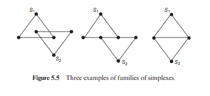
A triangle is a two-dimensional polygon with the minimum number of vertices. A tetrahedron is a three-dimensional polytope with the minimum number of vertices. They are the simplest polytopes with respect to the specific dimensions. They are both called simplexes. The concept of simplexes is a generalization of the notions of triangles and tetrahedrons. In general, a simplex is a polytope with the minimum number of vertices among all polytopes with certain dimension. For example, a point is a zero-dimensional simplex and a straight line segment is a one-dimensional simplex. The convex hull of linearly independent $n+1$ points in a Euclidean space is an $n$-dimensional simplex.
A face of a simplex $S$ is a simplex whose vertex set is a subset of vertices of $S$. A geometric simplicial complex is a family $\Gamma$ of simplexes satisfying the following conditions:
(a) For $S \in \Gamma$, every face of $S$ is in $\Gamma$.
(b) For $S, S^{\prime} \in \Gamma, S \cap S^{\prime}$ is a face for both $S$ and $S^{\prime}$.
(c) For $S, S^{\prime} \in \Gamma, S \cap S^{\prime}$ is also a simplex in $\Gamma$.
In Figure $5.5$, there are three examples; first two are not geometric simplicial complexes, the last one is.
Consider a set $X$ and a family $\Delta$ of subsets of $X . \Delta$ is called an (abstract) simplicial complex if for any $A$ in $\Delta$ every subset of $A$ also belongs to $\Delta$. Each member of $\Delta$ is called a face of $\Delta$. The dimension of a face $A$ is $|A|-1$. Any face of dimension 0 is called a vertex. For example, consider a set $X={a, b, c, d}$. The following family is a simplicial complex on $X$ :
$$
\begin{aligned}
\Delta=&{\emptyset,{a},{b},{c},{d},{a, b},{b, c},\
&{c, d},{d, a},{a, c},{a, b, c},{a, c, d}}
\end{aligned}
$$
The set ${a, b, c}$ is a face of dimension 2 and the empty set $\emptyset$ is a face of dimension $-1$.
计算复杂度理论代考
数学代写|计算复杂度理论代写Computational complexity theory代考|Algebraic Criterion
在本节中,我们提供了一些工具来证明布尔函数的难以捉摸。我们从一个简单的开始。
定理 5.10 具有奇数个真值赋值的布尔函数是难以捉摸的。
证明。常数函数F≡0和F≡1有 0 和2n分别为真值分配。因此,具有奇数个真值分配的布尔函数必须是非常数函数。如果F至少有两个变量和X一世是其中之一,那么真值分配的数量F是那些的总和F|X一世=0和F|X一世=1. 因此,无论是F|X一世=0或者F|X一世=1有奇数个真值赋值并且不是一个常数函数。因此,对于任何决策树计算F,跟踪具有奇数个真值分配的子树,我们将遇到从根到叶的路径中的所有变量。
定义
pF(ķ)=∑吨∈0,1nF(吨)ķ|吨吨,
在哪里|吨|是字符串中 l 的数量吨(回想一下,布尔赋值可以被视为二进制字符串)。很容易看出pF(1)是真值分配的数量F. 以下定理是定理的扩展5.10.
定理 5.11 对于布尔函数F的n变量,(ķ+1)n−D(F)∣pF(ķ).
证明。我们通过归纳证明这个定理D(F). 首先,我们注意到如果F≡0, 然后pF(ķ)=0而如果F≡1然后pF(ķ)=(ķ+1)n(由二项式定理)。这意味着该定理适用于D(F)=0. 现在,考虑F和D(F)>0和决策树吨深度的D(F)计算F. 不失一般性,假设根吨被标记为X1. 表示 $f_{0}=\left.f\right| {x {1}=0}一个ndf_{1}=\left.f\right| {x {1}=1}.吨H和npF(ķ)=∑吨∈0,1nF(吨)ķ|吨| =∑s∈0,1n−1F(0s)ķ|s|+∑s∈0,1n−1F(1s)ķ1+|s| =pF0(ķ)+ķpF1(ķ).ñ○吨和吨H一个吨D\left(f_{0}\right) \leq D(f)-1一个ndD\left(f_{1}\right) \leq D(f)-1.乙是吨H和一世nd在C吨一世○nH是p○吨H和s一世s,(k+1)^{n-1-D\left(f_{0}\right)} \mid p_{f_{0}}(k)一个nd(k+1)^{n-1-D\left(f_{1}\right)} \mid p_{f_{1}}(k).吨H在s,(k+1)^{nD(f)} \mid p_{f}(k)一个n一世米p○r吨一个n吨C○r○ll一个r是一世s一个sF○ll○在s.D和n○吨和\ mu (f) = p_ {f} (- 1) $。
数学代写|计算复杂度理论代写Computational complexity theory代考|Monotone Graph Properties
在本节中,我们证明了非平凡单调图属性的决策树复杂度的一般下界。
首先,让我们分析一下如何使用 Theorem5.13研究非平凡单调图的性质。请注意,每个图属性都是弱对称的,对于任何非平凡单调图属性,完整图必须具有该属性,而空图不得具有该属性。因此,如果我们想使用 Theorem5.13为了证明非平凡单调图属性的难以捉摸,我们只需要验证一个条件,即变量的数量是质数。然而,对于图属性,变量的数量是可能的边数,等于n(n−1)/2为了n顶点,它不是主要的力量n>3. 因此,定理5.13不能直接用于显示图形属性的难以捉摸。但是,它可以用于通过找到部分分配来建立稍微弱一点的结果,这样剩余变量的数量就会成为质数。以下引理源自这个想法。
引理5.16如果磷是有序图的非平凡单调性质n=2米, 然后D(磷)≥n2/4.
证明。让H一世成为不相交的联合2米−一世完整顺序图的副本2一世. 然后H0⊂H1⊂⋯⊂H米=ķn. 自从磷是非平凡的并且是单调的,H米有财产磷和H0没有财产磷. 因此,存在一个索引j这样Hj+1有财产磷和Hj没有财产磷. 分割Hj用顶点集分成两部分一个和乙,分别地,每一个都包含2米−j−1完整顺序图的不相交副本2j. 让ķ一个,乙是之间的完全二分图一个和乙. 然后Hj+1是一个子图Hj∪ķ一个,乙. 所以,Hj∪ķ一个,乙有财产磷. 现在,让F成为二分图上的函数一个和乙这样F在二分图中具有值 1G之间一个和乙当且仅当Hj∪G有财产磷. 然后F是一个非平凡单调弱对称函数|一个|⋅|乙|(=22米−2)变量。按定理5.13,D(磷)≥D(F)=22米−2=n2/4.
数学代写|计算复杂度理论代写Computational complexity theory代考|Topological Criterion
在本节中,我们将介绍一个强大的工具来研究单调布尔函数的难以捉摸性。我们从拓扑中的一些概念开始。
三角形是具有最少顶点数的二维多边形。四面体是具有最少顶点数的三维多面体。就特定维度而言,它们是最简单的多面体。它们都称为单纯形。单纯形的概念是三角形和四面体概念的概括。一般来说,单纯形是具有一定维度的所有多面体中顶点数最少的多面体。例如,点是零维单纯形,直线段是一维单纯形。线性独立的凸包n+1欧几里得空间中的点是n维单纯形。
单纯形的脸小号是一个单纯形,其顶点集是小号. 几何单纯复形是一个族Γ满足以下条件的单纯形:
(a) 对于小号∈Γ, 每一张脸小号在Γ.
(b) 为小号,小号′∈Γ,小号∩小号′是一张脸小号和小号′.
(c) 为小号,小号′∈Γ,小号∩小号′也是一个单纯形Γ.
如图5.5,有三个例子;前两个不是几何单纯复形,最后一个是。
考虑一个集合X和一个家庭Δ的子集X.Δ被称为(抽象)单纯复形,如果对于任何一个在Δ每个子集一个也属于Δ. 每个成员Δ被称为脸Δ. 一张脸的尺寸一个是|一个|−1. 任何维度为 0 的面称为顶点。例如,考虑一组X=一个,b,C,d. 下面的家庭是一个单纯复形X :
\begin{aligned} \Delta=&{\emptyset,{a},{b},{c},{d},{a, b},{b, c},\ &{c, d},{ d, a},{a, c},{a, b, c},{a, c, d}} \end{对齐}\begin{aligned} \Delta=&{\emptyset,{a},{b},{c},{d},{a, b},{b, c},\ &{c, d},{ d, a},{a, c},{a, b, c},{a, c, d}} \end{对齐}
套装一个,b,C是一个维度为 2 的面和空集∅是维度的脸−1.

统计代写请认准statistics-lab™. statistics-lab™为您的留学生涯保驾护航。
金融工程代写
金融工程是使用数学技术来解决金融问题。金融工程使用计算机科学、统计学、经济学和应用数学领域的工具和知识来解决当前的金融问题,以及设计新的和创新的金融产品。
非参数统计代写
非参数统计指的是一种统计方法,其中不假设数据来自于由少数参数决定的规定模型;这种模型的例子包括正态分布模型和线性回归模型。
广义线性模型代考
广义线性模型(GLM)归属统计学领域,是一种应用灵活的线性回归模型。该模型允许因变量的偏差分布有除了正态分布之外的其它分布。
术语 广义线性模型(GLM)通常是指给定连续和/或分类预测因素的连续响应变量的常规线性回归模型。它包括多元线性回归,以及方差分析和方差分析(仅含固定效应)。
有限元方法代写
有限元方法(FEM)是一种流行的方法,用于数值解决工程和数学建模中出现的微分方程。典型的问题领域包括结构分析、传热、流体流动、质量运输和电磁势等传统领域。
有限元是一种通用的数值方法,用于解决两个或三个空间变量的偏微分方程(即一些边界值问题)。为了解决一个问题,有限元将一个大系统细分为更小、更简单的部分,称为有限元。这是通过在空间维度上的特定空间离散化来实现的,它是通过构建对象的网格来实现的:用于求解的数值域,它有有限数量的点。边界值问题的有限元方法表述最终导致一个代数方程组。该方法在域上对未知函数进行逼近。[1] 然后将模拟这些有限元的简单方程组合成一个更大的方程系统,以模拟整个问题。然后,有限元通过变化微积分使相关的误差函数最小化来逼近一个解决方案。
tatistics-lab作为专业的留学生服务机构,多年来已为美国、英国、加拿大、澳洲等留学热门地的学生提供专业的学术服务,包括但不限于Essay代写,Assignment代写,Dissertation代写,Report代写,小组作业代写,Proposal代写,Paper代写,Presentation代写,计算机作业代写,论文修改和润色,网课代做,exam代考等等。写作范围涵盖高中,本科,研究生等海外留学全阶段,辐射金融,经济学,会计学,审计学,管理学等全球99%专业科目。写作团队既有专业英语母语作者,也有海外名校硕博留学生,每位写作老师都拥有过硬的语言能力,专业的学科背景和学术写作经验。我们承诺100%原创,100%专业,100%准时,100%满意。
随机分析代写
随机微积分是数学的一个分支,对随机过程进行操作。它允许为随机过程的积分定义一个关于随机过程的一致的积分理论。这个领域是由日本数学家伊藤清在第二次世界大战期间创建并开始的。
时间序列分析代写
随机过程,是依赖于参数的一组随机变量的全体,参数通常是时间。 随机变量是随机现象的数量表现,其时间序列是一组按照时间发生先后顺序进行排列的数据点序列。通常一组时间序列的时间间隔为一恒定值(如1秒,5分钟,12小时,7天,1年),因此时间序列可以作为离散时间数据进行分析处理。研究时间序列数据的意义在于现实中,往往需要研究某个事物其随时间发展变化的规律。这就需要通过研究该事物过去发展的历史记录,以得到其自身发展的规律。
回归分析代写
多元回归分析渐进(Multiple Regression Analysis Asymptotics)属于计量经济学领域,主要是一种数学上的统计分析方法,可以分析复杂情况下各影响因素的数学关系,在自然科学、社会和经济学等多个领域内应用广泛。
MATLAB代写
MATLAB 是一种用于技术计算的高性能语言。它将计算、可视化和编程集成在一个易于使用的环境中,其中问题和解决方案以熟悉的数学符号表示。典型用途包括:数学和计算算法开发建模、仿真和原型制作数据分析、探索和可视化科学和工程图形应用程序开发,包括图形用户界面构建MATLAB 是一个交互式系统,其基本数据元素是一个不需要维度的数组。这使您可以解决许多技术计算问题,尤其是那些具有矩阵和向量公式的问题,而只需用 C 或 Fortran 等标量非交互式语言编写程序所需的时间的一小部分。MATLAB 名称代表矩阵实验室。MATLAB 最初的编写目的是提供对由 LINPACK 和 EISPACK 项目开发的矩阵软件的轻松访问,这两个项目共同代表了矩阵计算软件的最新技术。MATLAB 经过多年的发展,得到了许多用户的投入。在大学环境中,它是数学、工程和科学入门和高级课程的标准教学工具。在工业领域,MATLAB 是高效研究、开发和分析的首选工具。MATLAB 具有一系列称为工具箱的特定于应用程序的解决方案。对于大多数 MATLAB 用户来说非常重要,工具箱允许您学习和应用专业技术。工具箱是 MATLAB 函数(M 文件)的综合集合,可扩展 MATLAB 环境以解决特定类别的问题。可用工具箱的领域包括信号处理、控制系统、神经网络、模糊逻辑、小波、仿真等。