标签: MINE7034

金融代写|量化风险管理代写Quantitative Risk Management代考|PROJMGNT1002

如果你也在 怎样代写量化风险管理Quantitative Risk Management这个学科遇到相关的难题,请随时右上角联系我们的24/7代写客服。

项目管理中的定量风险管理是将风险对项目的影响转换为数字的过程。这种数字信息经常被用来确定项目的成本和时间应急措施。

statistics-lab™ 为您的留学生涯保驾护航 在代写量化风险管理Quantitative Risk Management方面已经树立了自己的口碑, 保证靠谱, 高质且原创的统计Statistics代写服务。我们的专家在代写量化风险管理Quantitative Risk Management代写方面经验极为丰富,各种代写量化风险管理Quantitative Risk Management相关的作业也就用不着说。

我们提供的量化风险管理Quantitative Risk Management及其相关学科的代写,服务范围广, 其中包括但不限于:

  • Statistical Inference 统计推断
  • Statistical Computing 统计计算
  • Advanced Probability Theory 高等概率论
  • Advanced Mathematical Statistics 高等数理统计学
  • (Generalized) Linear Models 广义线性模型
  • Statistical Machine Learning 统计机器学习
  • Longitudinal Data Analysis 纵向数据分析
  • Foundations of Data Science 数据科学基础
金融代写|量化风险管理代写Quantitative Risk Management代考|PROJMGNT1002

金融代写|量化风险管理代写Quantitative Risk Management代考|Risks faced by a financial firm

Decrease in the value of the investments on the asset side of the balance sheet (e.g. losses from securities trading or credit risk).

  • Maturity mismatch (large parts of the assets are relatively illiquid (longterm) whereas large parts of the liabilities are rather short-term obligations. This can lead to a default of a solvent bank or a bank run).
  • The prime risk for an insurer is insolvency (risk that claims of policy holders cannot be met). On the asset side, risks are similar to those of a bank. On the liability side, the main risk is that reserves are insufficient
  • to cover future claim payments. Note that the liabilities of a life insurer are of a long-term nature and subject to multiple categories of risk (e.g. interest rate risk, inflation risk and longevity risk).
  • So risk is found on both sides of the balance sheet and thus RM should not focus on the asset side alone.
  • There are different notions of capital. One distinguishes:
    Equity capital $\quad-$ Value of assets – debt;
  • Measures the firm’s value to its shareholders;
  • Can be split into shareholder capital (initial capital invested in the firm) and retained earnings (accumulated earnings not paid to shareholders).
    Regulatory capital – Capital required according to regulatory rules;
  • For European insurance firms: Minimum (MCR) and solvency capital requirements (SCR);
  • A regulatory framework also specifies the capital quality. One distinguishes Tier 1 capital (i.e. shareholder capital + retained earnings; can act in full as buffer) and Tier 2 capital (includes other positions on the balance sheet).
  • Capital required to control the probability of becoming insolvent (typically over one year);
  • Internal assessment of risk capital;
  • Aims at a holistic view (assets and liabilities) and works with fair values of balance sheet items.

金融代写|量化风险管理代写Quantitative Risk Management代考|Modelling value and value change

We set up a general mathematical model for (changes in) value caused by financial risks. To this end we work on a probability space $(\Omega, \mathcal{F}, \mathbb{P})$ and consider a risk or loss as a random variable $X: \Omega \rightarrow \mathbb{R}($ or: $L$ ).

  • Consider a portfolio of assets and possibly liabilities. The value of the portfolio at time $t$ (today) is denoted by $V_t$ (a random variable; assumed to be known at $t$; its $d f$ is typically not trivial to determine!).
  • We consider a given time horizon $\Delta t$ and assume:
    1) the portfolio composition remains fixed over $\Delta t$;
    2) there are no intermediate payments during $\Delta t$
    $\Rightarrow$ Fine for small $\Delta t$ but unlikely to hold for large $\Delta t$.
  • The change in value of the portfolio is given by
    $$
    \Delta V_{t+1}=V_{t+1}-V_t
    $$
    and we define the (random) loss by the sign-adjusted value change
    $$
    L_{t+1}=-\Delta V_{t+1}
    $$
    (as QRM is mainly concerned with losses).

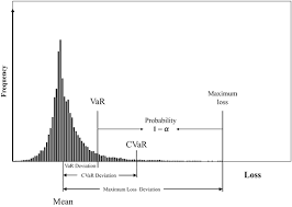
1) The distribution of $L_{t+1}$ is called loss distribution.
2) Practitioners often consider the profit-and-loss $(P \& L)$ distribution which is the distribution of $-L_{t+1}=\Delta V_{t+1}$.
3) For longer time intervals, $\Delta V_{t+1}=V_{t+1} /(1+r)-V_t$ ( $r=$ risk-free interest rate) would be more appropriate, but we will mostly neglect this issue.

  • $V_t$ is typically modelled as a function $f$ of time $t$ and a $d$-dimensional random vector $\boldsymbol{Z}=\left(Z_{t, 1}, \ldots, Z_{t, d}\right)$ of risk factors, that is,
    $$
    V_t=f\left(t, \boldsymbol{Z}t\right) \quad \text { (mapping of risks) } $$ for some measurable $f: \mathbb{R}{+} \times \mathbb{R}^d \rightarrow \mathbb{R}$. The choice of $f$ and $\boldsymbol{Z}_t$ is problem-specific (typically known, but possibly difficult to evaluate).
  • It is often convenient to work with the risk-factor changes
    $$
    \boldsymbol{X}{t+1}=\boldsymbol{Z}{t+1}-\boldsymbol{Z}t . $$ We can rewrite $L{t+1}$ in terms of $\boldsymbol{X}{t+1}$ via $$ \begin{aligned} L{t+1} & =-\left(V_{t+1}-V_t\right)=-\left(f\left(t+1, \boldsymbol{Z}{t+1}\right)-f\left(t, \boldsymbol{Z}_t\right)\right) \ & =-\left(f\left(t+1, \boldsymbol{Z}_t+\boldsymbol{X}{t+1}\right)-f\left(t, \boldsymbol{Z}t\right)\right) \end{aligned} $$ We see that the loss $d f$ is determined by the loss df of $X{t+1}$. We will thus also write $L_{t+1}=L\left(\boldsymbol{X}_{t+1}\right)$, where $L(\boldsymbol{x})=-\left(f\left(t+1, \boldsymbol{Z}_t+\boldsymbol{x}\right)-f\left(t, \boldsymbol{Z}_t\right)\right)$ is known as loss operator.
金融代写|量化风险管理代写Quantitative Risk Management代考|PROJMGNT1002

量化风险管理代考

金融代写|量化风险管理代写Quantitative Risk Management代考|Risks faced by a financial firm

资产负债表资产端的投资价值下降(例如,证券交易损失或信用风险)。

  • 期限错配(大部分资产流动性相对较差(长期),而大部分负债是相当短期的债务。这可能导致有偿付能力的银行违约或银行挤兑)。
  • 保险公司面临的主要风险是资不抵债(无法满足保单持有人索赔的风险)。在资产方面,风险类似于银行的风险。负债端,主要风险是准备金不足
  • 以支付未来的理赔费用。请注意,人寿保险公司的负债具有长期性质,并受到多种风险的影响(例如利率风险、通胀风险和长寿风险)。
  • 因此,资产负债表的两边都存在风险,因此 RM 不应只关注资产方面。
  • 有不同的资本概念。一区分:
    股权资本−资产价值——债务;
  • 衡量公司对其股东的价值;
  • 可以分为股东资本(投资于公司的初始资本)和留存收益(未支付给股东的累计收益)。
    监管资本——监管规定要求的资本;
  • 对于欧洲保险公司:最低 (MCR) 和偿付能力资本要求 (SCR);
  • 监管框架还规定了资本质量。一种区分一级资本(即股东资本+留存收益;可以完全作为缓冲)和二级资本(包括资产负债表上的其他头寸)。
  • 控制破产可能性所需的资本(通常超过一年);
  • 风险资本内部评估;
  • 以整体观点(资产和负债)为目标,并处理资产负债表项目的公允价值。

金融代写|量化风险管理代写Quantitative Risk Management代考|Modelling value and value change

我们为金融风险引起的价值 (变化) 建立了一个通用的数学模型。为此,我们在概率空间上工作 $(\Omega, \mathcal{F}, \mathbb{P})$ 并将风险或损失视为随机变量 $X: \Omega \rightarrow \mathbb{R}($ 或者: $L$ ).

  • 考虑一个资产组合,可能还有负债。投资组合当时的价值 $t$ (今天) 表示为 $V_t$ (一个随机变量; 假设 在 $t ;$ 它的 $d f$ 确定起来通常不是微不足道的))。
  • 我们考虑给定的时间范围 $\Delta t$ 并假设:
    1) 投资组合构成在 $\Delta t$;
    2)期间没有中间付款 $\Delta t$
    $\Rightarrow$ 适合小的 $\Delta t$ 但不太可能长期持有 $\Delta t$.
  • 投资组合价值的变化由下式给出
    $$
    \Delta V_{t+1}=V_{t+1}-V_t
    $$
    我们通过符号调整后的值变化来定义 (随机) 损失
    $$
    L_{t+1}=-\Delta V_{t+1}
    $$
    (因为 $\mathrm{QRM}$ 主要关注损失) 。
    1) 分布 $L_{t+1}$ 称为损失分布。
    2) 从业者往往考虑盈亏 $(P \& L)$ 分布这是分布 $-L_{t+1}=\Delta V_{t+1}$.
    3) 对于更长的时间间隔, $\Delta V_{t+1}=V_{t+1} /(1+r)-V_t(r=$ 无风险利率) 会更合适,但我们大多会 忽略这个问题。
  • $V_t$ 通常被建模为一个函数 $f$ 时间的 $t$ 和一个 $d$ 维随机向量 $\boldsymbol{Z}=\left(Z_{t, 1}, \ldots, Z_{t, d}\right)$ 的风险因素,即
    $$
    V_t=f(t, \boldsymbol{Z} t) \quad \text { (mapping of risks) }
    $$
    对于一些可测量的 $f: \mathbb{R}+\times \mathbb{R}^d \rightarrow \mathbb{R}$. 的选择 $f$ 和 $Z_t$ 是特定于问题的(通常是已知的,但可能难 以评估)。
  • 处理风险因素变化通常很方便
    $$
    \boldsymbol{X} t+1=\boldsymbol{Z} t+1-\boldsymbol{Z} t .
    $$
    我们可以重写 $L t+1$ 按照 $\boldsymbol{X} t+1$ 通过
    $$
    L t+1=-\left(V_{t+1}-V_t\right)=-\left(f(t+1, \boldsymbol{Z} t+1)-f\left(t, \boldsymbol{Z}t\right)\right) \quad=-\left(f \left(t+1, \boldsymbol{Z}_t+\boldsymbol{X} t\right.\right. $$ 我们看到损失 $d f$ 由损失 df 决定 $X t+1$. 因此我们也将写 $L{t+1}=L\left(\boldsymbol{X}_{t+1}\right)$ ,在哪里$L(\boldsymbol{x})=-\left(f\left(t+1, \boldsymbol{Z}_t+\boldsymbol{x}\right)-f\left(t, \boldsymbol{Z}_t\right)\right)$ 被称为损失算子。
金融代写|量化风险管理代写Quantitative Risk Management代考 请认准statistics-lab™

统计代写请认准statistics-lab™. statistics-lab™为您的留学生涯保驾护航。

金融工程代写

金融工程是使用数学技术来解决金融问题。金融工程使用计算机科学、统计学、经济学和应用数学领域的工具和知识来解决当前的金融问题,以及设计新的和创新的金融产品。

非参数统计代写

非参数统计指的是一种统计方法,其中不假设数据来自于由少数参数决定的规定模型;这种模型的例子包括正态分布模型和线性回归模型。

广义线性模型代考

广义线性模型(GLM)归属统计学领域,是一种应用灵活的线性回归模型。该模型允许因变量的偏差分布有除了正态分布之外的其它分布。

术语 广义线性模型(GLM)通常是指给定连续和/或分类预测因素的连续响应变量的常规线性回归模型。它包括多元线性回归,以及方差分析和方差分析(仅含固定效应)。

有限元方法代写

有限元方法(FEM)是一种流行的方法,用于数值解决工程和数学建模中出现的微分方程。典型的问题领域包括结构分析、传热、流体流动、质量运输和电磁势等传统领域。

有限元是一种通用的数值方法,用于解决两个或三个空间变量的偏微分方程(即一些边界值问题)。为了解决一个问题,有限元将一个大系统细分为更小、更简单的部分,称为有限元。这是通过在空间维度上的特定空间离散化来实现的,它是通过构建对象的网格来实现的:用于求解的数值域,它有有限数量的点。边界值问题的有限元方法表述最终导致一个代数方程组。该方法在域上对未知函数进行逼近。[1] 然后将模拟这些有限元的简单方程组合成一个更大的方程系统,以模拟整个问题。然后,有限元通过变化微积分使相关的误差函数最小化来逼近一个解决方案。

tatistics-lab作为专业的留学生服务机构,多年来已为美国、英国、加拿大、澳洲等留学热门地的学生提供专业的学术服务,包括但不限于Essay代写,Assignment代写,Dissertation代写,Report代写,小组作业代写,Proposal代写,Paper代写,Presentation代写,计算机作业代写,论文修改和润色,网课代做,exam代考等等。写作范围涵盖高中,本科,研究生等海外留学全阶段,辐射金融,经济学,会计学,审计学,管理学等全球99%专业科目。写作团队既有专业英语母语作者,也有海外名校硕博留学生,每位写作老师都拥有过硬的语言能力,专业的学科背景和学术写作经验。我们承诺100%原创,100%专业,100%准时,100%满意。

随机分析代写


随机微积分是数学的一个分支,对随机过程进行操作。它允许为随机过程的积分定义一个关于随机过程的一致的积分理论。这个领域是由日本数学家伊藤清在第二次世界大战期间创建并开始的。

时间序列分析代写

随机过程,是依赖于参数的一组随机变量的全体,参数通常是时间。 随机变量是随机现象的数量表现,其时间序列是一组按照时间发生先后顺序进行排列的数据点序列。通常一组时间序列的时间间隔为一恒定值(如1秒,5分钟,12小时,7天,1年),因此时间序列可以作为离散时间数据进行分析处理。研究时间序列数据的意义在于现实中,往往需要研究某个事物其随时间发展变化的规律。这就需要通过研究该事物过去发展的历史记录,以得到其自身发展的规律。

回归分析代写

多元回归分析渐进(Multiple Regression Analysis Asymptotics)属于计量经济学领域,主要是一种数学上的统计分析方法,可以分析复杂情况下各影响因素的数学关系,在自然科学、社会和经济学等多个领域内应用广泛。

MATLAB代写

MATLAB 是一种用于技术计算的高性能语言。它将计算、可视化和编程集成在一个易于使用的环境中,其中问题和解决方案以熟悉的数学符号表示。典型用途包括:数学和计算算法开发建模、仿真和原型制作数据分析、探索和可视化科学和工程图形应用程序开发,包括图形用户界面构建MATLAB 是一个交互式系统,其基本数据元素是一个不需要维度的数组。这使您可以解决许多技术计算问题,尤其是那些具有矩阵和向量公式的问题,而只需用 C 或 Fortran 等标量非交互式语言编写程序所需的时间的一小部分。MATLAB 名称代表矩阵实验室。MATLAB 最初的编写目的是提供对由 LINPACK 和 EISPACK 项目开发的矩阵软件的轻松访问,这两个项目共同代表了矩阵计算软件的最新技术。MATLAB 经过多年的发展,得到了许多用户的投入。在大学环境中,它是数学、工程和科学入门和高级课程的标准教学工具。在工业领域,MATLAB 是高效研究、开发和分析的首选工具。MATLAB 具有一系列称为工具箱的特定于应用程序的解决方案。对于大多数 MATLAB 用户来说非常重要,工具箱允许您学习应用专业技术。工具箱是 MATLAB 函数(M 文件)的综合集合,可扩展 MATLAB 环境以解决特定类别的问题。可用工具箱的领域包括信号处理、控制系统、神经网络、模糊逻辑、小波、仿真等。

R语言代写问卷设计与分析代写
PYTHON代写回归分析与线性模型代写
MATLAB代写方差分析与试验设计代写
STATA代写机器学习/统计学习代写
SPSS代写计量经济学代写
EVIEWS代写时间序列分析代写
EXCEL代写深度学习代写
SQL代写各种数据建模与可视化代写

金融代写|量化风险管理代写Quantitative Risk Management代考|PROJMGNT5004

如果你也在 怎样代写量化风险管理Quantitative Risk Management这个学科遇到相关的难题,请随时右上角联系我们的24/7代写客服。

项目管理中的定量风险管理是将风险对项目的影响转换为数字的过程。这种数字信息经常被用来确定项目的成本和时间应急措施。

statistics-lab™ 为您的留学生涯保驾护航 在代写量化风险管理Quantitative Risk Management方面已经树立了自己的口碑, 保证靠谱, 高质且原创的统计Statistics代写服务。我们的专家在代写量化风险管理Quantitative Risk Management代写方面经验极为丰富,各种代写量化风险管理Quantitative Risk Management相关的作业也就用不着说。

我们提供的量化风险管理Quantitative Risk Management及其相关学科的代写,服务范围广, 其中包括但不限于:

  • Statistical Inference 统计推断
  • Statistical Computing 统计计算
  • Advanced Probability Theory 高等概率论
  • Advanced Mathematical Statistics 高等数理统计学
  • (Generalized) Linear Models 广义线性模型
  • Statistical Machine Learning 统计机器学习
  • Longitudinal Data Analysis 纵向数据分析
  • Foundations of Data Science 数据科学基础
金融代写|量化风险管理代写Quantitative Risk Management代考|PROJMGNT5004

金融代写|量化风险管理代写Quantitative Risk Management代考|Why manage financial risk

  • Society (single customers and as a whole (systemic risk)) relies on the stability of the banking and insurance system.
  • This is related to systemic importance of the company in question (size and connectivity to other firms). Considering some firms as too big to fail creates a moral hazard (should be avoided!) since the management of such a firm may take more risk knowing that it would be bailed out in a crisis.
  • Better risk management can reduce the risk of company failure and protect customers and policyholders. However, regulation must be designed with care and should not promote herding, procyclical behaviour or other forms of endogenous risk that could result in a systemic crisis.
  • We treat QRM as a quantitative science using the language of mathematics in general, and probability and statistics in particular.
  • Probability and statistics provide us with a suitable language and with appropriate concepts for describing financial risks.
  • We also point out assumptions and limitations of the methodology used.
  • The $Q$ in QRM is an essential part of the RM process. We believe it remains (if applied correctly and honestly) a part of the solution to managing risk (not the problem). See also Shreve (2008):
    “Don’t blame the quants. Hire good ones instead and listen to them.”

金融代写|量化风险管理代写Quantitative Risk Management代考|The nature of the challenge

  • Our approach to QRM has two main strands:
  • Put current practice onto a firmer mathematical ground;
  • Put together techniques and tools which go beyond current practice and address some of the deficiencies.
  • In particular, some of the challenges of QRM are:
  • Extremes matter.
  • Interdependence and concentration of risks.
  • The problem of scale (models for all risk factors may not be feasible).
  • Interdisciplinarity.
  • Communication and education.

Balance sheet equation: Assets $=$ Liabilities $=$ Debt $+$ Equity. If equity $>0$, the company is solvent, otherwise insolvent.

Valuation of the items on the balance sheet is a non-trivial task.

  • Amortized cost accounting values a position a book value at its inception and this is carried forward/progressively reduced over time.

Fair-value accounting values assets at prices they are sold and liabilities at prices that would have to be paid in the market. This can be challenging for non-traded or illiquid assets or liabilities.

There is a tendency in the industry to move towards fair-value accounting. Market consistent valuation in Solvency II follows similar principles.

金融代写|量化风险管理代写Quantitative Risk Management代考|PROJMGNT5004

量化风险管理代考

金融代写|量化风险管理代写Quantitative Risk Management代考|Why manage financial risk

  • 社会(单一客户和整体(系统性风险))依赖于银行和保险体系的稳定性。
  • 这与相关公司的系统重要性(规模和与其他公司的联系)有关。将某些公司视为太大而不能倒闭会产生道德风险(应该避免!),因为此类公司的管理层可能会承担更多风险,因为他们知道自己会在危机中得到救助。
  • 更好的风险管理可以降低公司倒闭的风险并保护客户和保单持有人。然而,监管必须谨慎设计,不应助长羊群行为、顺周期行为或其他可能导致系统性危机的内生风险形式。
  • 我们将 QRM 视为一门使用一般数学语言,特别是概率和统计语言的定量科学。
  • 概率和统计为我们提供了一种合适的语言和合适的概念来描述金融风险。
  • 我们还指出了所用方法的假设和局限性。
  • 这问在 QRM 中是 RM 过程的重要组成部分。我们相信它仍然(如果正确和诚实地应用)是管理风险(而不是问题)的解决方案的一部分。另见 Shreve (2008):
    “不要责怪宽客。相反,请聘请优秀的人并听取他们的意见。”

金融代写|量化风险管理代写Quantitative Risk Management代考|The nature of the challenge

  • 我们的 QRM 方法有两个主要方面:
  • 将当前的实践置于更坚实的数学基础上;
  • 将超越当前实践的技术和工具放在一起并解决一些缺陷。
  • 特别是,QRM 的一些挑战是:
  • 极端很重要。
  • 相互依赖和风险集中。
  • 规模问题(所有风险因素的模型可能不可行)。
  • 跨学科。
  • 沟通和教育。

资产负债表等式:资产=负债=债务+公平。如果股权>0,公司有偿付能力,否则资不抵债。

对资产负债表上的项目进行估值是一项非常重要的任务。

  • 摊余成本会计对头寸的初始账面价值进行估值,并随着时间的推移结转/逐渐减少。

公允价值会计按资产的出售价格对资产进行估值,对负债的估值则按必须在市场上支付的价格进行。这对于非交易或非流动性资产或负债来说可能具有挑战性。

该行业有转向公允价值会计的趋势。Solvency II 中的市场一致估值遵循类似的原则。

金融代写|量化风险管理代写Quantitative Risk Management代考 请认准statistics-lab™

统计代写请认准statistics-lab™. statistics-lab™为您的留学生涯保驾护航。

金融工程代写

金融工程是使用数学技术来解决金融问题。金融工程使用计算机科学、统计学、经济学和应用数学领域的工具和知识来解决当前的金融问题,以及设计新的和创新的金融产品。

非参数统计代写

非参数统计指的是一种统计方法,其中不假设数据来自于由少数参数决定的规定模型;这种模型的例子包括正态分布模型和线性回归模型。

广义线性模型代考

广义线性模型(GLM)归属统计学领域,是一种应用灵活的线性回归模型。该模型允许因变量的偏差分布有除了正态分布之外的其它分布。

术语 广义线性模型(GLM)通常是指给定连续和/或分类预测因素的连续响应变量的常规线性回归模型。它包括多元线性回归,以及方差分析和方差分析(仅含固定效应)。

有限元方法代写

有限元方法(FEM)是一种流行的方法,用于数值解决工程和数学建模中出现的微分方程。典型的问题领域包括结构分析、传热、流体流动、质量运输和电磁势等传统领域。

有限元是一种通用的数值方法,用于解决两个或三个空间变量的偏微分方程(即一些边界值问题)。为了解决一个问题,有限元将一个大系统细分为更小、更简单的部分,称为有限元。这是通过在空间维度上的特定空间离散化来实现的,它是通过构建对象的网格来实现的:用于求解的数值域,它有有限数量的点。边界值问题的有限元方法表述最终导致一个代数方程组。该方法在域上对未知函数进行逼近。[1] 然后将模拟这些有限元的简单方程组合成一个更大的方程系统,以模拟整个问题。然后,有限元通过变化微积分使相关的误差函数最小化来逼近一个解决方案。

tatistics-lab作为专业的留学生服务机构,多年来已为美国、英国、加拿大、澳洲等留学热门地的学生提供专业的学术服务,包括但不限于Essay代写,Assignment代写,Dissertation代写,Report代写,小组作业代写,Proposal代写,Paper代写,Presentation代写,计算机作业代写,论文修改和润色,网课代做,exam代考等等。写作范围涵盖高中,本科,研究生等海外留学全阶段,辐射金融,经济学,会计学,审计学,管理学等全球99%专业科目。写作团队既有专业英语母语作者,也有海外名校硕博留学生,每位写作老师都拥有过硬的语言能力,专业的学科背景和学术写作经验。我们承诺100%原创,100%专业,100%准时,100%满意。

随机分析代写


随机微积分是数学的一个分支,对随机过程进行操作。它允许为随机过程的积分定义一个关于随机过程的一致的积分理论。这个领域是由日本数学家伊藤清在第二次世界大战期间创建并开始的。

时间序列分析代写

随机过程,是依赖于参数的一组随机变量的全体,参数通常是时间。 随机变量是随机现象的数量表现,其时间序列是一组按照时间发生先后顺序进行排列的数据点序列。通常一组时间序列的时间间隔为一恒定值(如1秒,5分钟,12小时,7天,1年),因此时间序列可以作为离散时间数据进行分析处理。研究时间序列数据的意义在于现实中,往往需要研究某个事物其随时间发展变化的规律。这就需要通过研究该事物过去发展的历史记录,以得到其自身发展的规律。

回归分析代写

多元回归分析渐进(Multiple Regression Analysis Asymptotics)属于计量经济学领域,主要是一种数学上的统计分析方法,可以分析复杂情况下各影响因素的数学关系,在自然科学、社会和经济学等多个领域内应用广泛。

MATLAB代写

MATLAB 是一种用于技术计算的高性能语言。它将计算、可视化和编程集成在一个易于使用的环境中,其中问题和解决方案以熟悉的数学符号表示。典型用途包括:数学和计算算法开发建模、仿真和原型制作数据分析、探索和可视化科学和工程图形应用程序开发,包括图形用户界面构建MATLAB 是一个交互式系统,其基本数据元素是一个不需要维度的数组。这使您可以解决许多技术计算问题,尤其是那些具有矩阵和向量公式的问题,而只需用 C 或 Fortran 等标量非交互式语言编写程序所需的时间的一小部分。MATLAB 名称代表矩阵实验室。MATLAB 最初的编写目的是提供对由 LINPACK 和 EISPACK 项目开发的矩阵软件的轻松访问,这两个项目共同代表了矩阵计算软件的最新技术。MATLAB 经过多年的发展,得到了许多用户的投入。在大学环境中,它是数学、工程和科学入门和高级课程的标准教学工具。在工业领域,MATLAB 是高效研究、开发和分析的首选工具。MATLAB 具有一系列称为工具箱的特定于应用程序的解决方案。对于大多数 MATLAB 用户来说非常重要,工具箱允许您学习应用专业技术。工具箱是 MATLAB 函数(M 文件)的综合集合,可扩展 MATLAB 环境以解决特定类别的问题。可用工具箱的领域包括信号处理、控制系统、神经网络、模糊逻辑、小波、仿真等。

R语言代写问卷设计与分析代写
PYTHON代写回归分析与线性模型代写
MATLAB代写方差分析与试验设计代写
STATA代写机器学习/统计学习代写
SPSS代写计量经济学代写
EVIEWS代写时间序列分析代写
EXCEL代写深度学习代写
SQL代写各种数据建模与可视化代写

金融代写|量化风险管理代写Quantitative Risk Management代考|FNCE90082

如果你也在 怎样代写量化风险管理Quantitative Risk Management这个学科遇到相关的难题,请随时右上角联系我们的24/7代写客服。

项目管理中的定量风险管理是将风险对项目的影响转换为数字的过程。这种数字信息经常被用来确定项目的成本和时间应急措施。

statistics-lab™ 为您的留学生涯保驾护航 在代写量化风险管理Quantitative Risk Management方面已经树立了自己的口碑, 保证靠谱, 高质且原创的统计Statistics代写服务。我们的专家在代写量化风险管理Quantitative Risk Management代写方面经验极为丰富,各种代写量化风险管理Quantitative Risk Management相关的作业也就用不着说。

我们提供的量化风险管理Quantitative Risk Management及其相关学科的代写,服务范围广, 其中包括但不限于:

  • Statistical Inference 统计推断
  • Statistical Computing 统计计算
  • Advanced Probability Theory 高等概率论
  • Advanced Mathematical Statistics 高等数理统计学
  • (Generalized) Linear Models 广义线性模型
  • Statistical Machine Learning 统计机器学习
  • Longitudinal Data Analysis 纵向数据分析
  • Foundations of Data Science 数据科学基础
金融代写|量化风险管理代写Quantitative Risk Management代考|FNCE90082

金融代写|量化风险管理代写Quantitative Risk Management代考|Risk and randomness

  • The Concise Oxford English Dictionary: “hazard, a chance of bad consequences, loss or exposure to mischance”.
  • McNeil, Frey, and Embrechts (2005): “any event or action that may adversely affect an organization’s ability to achieve its objectives and execute its strategies”.
  • No single one-sentence definition captures all aspects of risk.
    For us: risk $=$ chance of loss $\Rightarrow$ randomness

We will mostly model situations in which an investor holds today an asset with an uncertain future value.

We use probabilistic notions (random variables, random vectors, distributions, stochastic processes) and statistical tools. In particular, we assume to work on a probability space $(\Omega, \mathcal{F}, \mathbb{P})$; see Kolmogorov (1933).

There are various types of risks. We focus on (those affected by regulation):
Market risk Risk of loss in a financial position due to changes in the underlying components (e.g. stock/bond/commodity prices)
Credit risk Risk of a counterparty failing to meet its obligations (default), i.e. the risk of not receiving promised repayments (e.g. loans/bonds).
Operational risk (OpRisk) Risk of loss resulting from inadequate or failed internal processes, people and systems or from external events (e.g. fraud, fat-finger trades, earthquakes).

There are many other types of risks such as liquidity risk, underwriting risk, or model risk (the risk of using a misspecified or inappropriate model for measuring risk; model risk is always present to some degree).

金融代写|量化风险管理代写Quantitative Risk Management代考|Measurement and management

  • Suppose we hold a portfolio of $d$ investments with weights $w_1, \ldots, w_d$. Let $X_j$ denote the change in value of the $j$ th investment. The change in value – profit and loss $(P \& L)$ – of the portfolio over a given holding period is then
    $$
    X=\sum_{j=1}^d w_j X_j
    $$
    Measuring the risk now consists of determining the distribution function $F$ (or functionals of it, e.g. mean, variance, $\alpha$-quantiles $F^{\leftarrow}(\alpha)=$ $\inf {x \in \mathbb{R}: F(x) \geq \alpha})$.
  • To this end, we need a properly calibrated joint model for $\boldsymbol{X}=$ $\left(X_1, \ldots, X_d\right)$. Statistical estimates of $F$ or one of its functionals are obtained based on historical observations of this model.

What is RM? Kloman (1990) writes:
“RM is a discipline for living with the possibility that future events may cause adverse effects.”
$\Rightarrow$ It is about ensuring resilience to future events.
Note that financial firms are not passive/defensive towards risk, banks and insurers actively/willingly take risks because they seek a return. RM thus belongs to their core competence.
What does managing risks involve?
Determine the capital to hold to absorb losses, both for regulatory purposes (to comply with regulators) and economic capital purposes (to survive as a company).

  • Ensuring portfolios are well diversified.
  • Optimizing portfolios according to risk-return considerations.
金融代写|量化风险管理代写Quantitative Risk Management代考|FNCE90082

量化风险管理代考

金融代写|量化风险管理代写Quantitative Risk Management代考|Risk and randomness

  • 简明牛津英语词典:“hazard, a chance of bad consequences, loss or exposure to mischance”。
  • McNeil、Frey 和 Embrechts(2005 年):“任何可能对组织实现其目标和执行其战略的能力产生不利影响的事件或行动”。
  • 没有一个单一的一句话定义可以涵盖风险的所有方面。
    对我们来说:风险=损失的机会⇒随机性

我们将主要模拟投资者今天持有未来价值不确定的资产的情况。

我们使用概率概念(随机变量、随机向量、分布、随机过程)和统计工具。特别是,我们假设在概率空间上工作(哦,F,P); 参见 Kolmogorov (1933)。

存在各种类型的风险。我们关注(受监管影响的那些):
市场风险 因基础成分(例如股票/债券/商品价格)变化而导致财务状况损失的风险
信用风险 交易对手未能履行其义务(违约)的风险,即未收到承诺的还款(例如贷款/债券)的风险。
操作风险 (OpRisk) 因内部流程、人员和系统不完善或故障或外部事件(例如欺诈、胖手指交易、地震)导致损失的风险。

还有许多其他类型的风险,例如流动性风险、承保风险或模型风险(使用错误指定或不适当的模型来衡量风险的风险;模型风险总是在某种程度上存在)。

金融代写|量化风险管理代写Quantitative Risk Management代考|Measurement and management

  • 假设我们持有一个投资组合 $d$ 权重投资 $w_1, \ldots, w_d$. 让 $X_j$ 表示值的变化 $j$ 第投资。价值的变化一损益 $(P \& L)$ – 在给定的持有期内,投资组合的
    $$
    X=\sum_{j=1}^d w_j X_j
    $$
    衡量风险现在包括确定分布函数 $F$ (或其泛函,例如均值、方差、 $\alpha$-分位数 $F^{\leftarrow}(\alpha)=$ $\inf x \in \mathbb{R}: F(x) \geq \alpha)$.
  • 为此,我们需要一个适当校准的联合模型 $\boldsymbol{X}=\left(X_1, \ldots, X_d\right)$. 的统计估计 $F$ 或其功能之一是根据 对该模型的历史观察获得的。
    什么是马币? Kloman (1990) 写道:
    “RM 是一种与末来事件可能造成不利影响的可能性一起生活的学科。”
    $\Rightarrow$ 它是关于确保对末来事件的弹性。
    请注意,金融公司并非被动/防御风险,银行和保险公司主动/愿意承担风险,因为他们寻求回报。RM因此 属于他们的核心竞争力。
    管理风险涉及什么?
    出于监管目的(遵守监管机构)和经济资本目的(作为公司生存)确定持有以吸收损失的资本。
  • 确保投资组合多元化。
  • 根据风险回报考虑优化投资组合。
金融代写|量化风险管理代写Quantitative Risk Management代考 请认准statistics-lab™

统计代写请认准statistics-lab™. statistics-lab™为您的留学生涯保驾护航。

金融工程代写

金融工程是使用数学技术来解决金融问题。金融工程使用计算机科学、统计学、经济学和应用数学领域的工具和知识来解决当前的金融问题,以及设计新的和创新的金融产品。

非参数统计代写

非参数统计指的是一种统计方法,其中不假设数据来自于由少数参数决定的规定模型;这种模型的例子包括正态分布模型和线性回归模型。

广义线性模型代考

广义线性模型(GLM)归属统计学领域,是一种应用灵活的线性回归模型。该模型允许因变量的偏差分布有除了正态分布之外的其它分布。

术语 广义线性模型(GLM)通常是指给定连续和/或分类预测因素的连续响应变量的常规线性回归模型。它包括多元线性回归,以及方差分析和方差分析(仅含固定效应)。

有限元方法代写

有限元方法(FEM)是一种流行的方法,用于数值解决工程和数学建模中出现的微分方程。典型的问题领域包括结构分析、传热、流体流动、质量运输和电磁势等传统领域。

有限元是一种通用的数值方法,用于解决两个或三个空间变量的偏微分方程(即一些边界值问题)。为了解决一个问题,有限元将一个大系统细分为更小、更简单的部分,称为有限元。这是通过在空间维度上的特定空间离散化来实现的,它是通过构建对象的网格来实现的:用于求解的数值域,它有有限数量的点。边界值问题的有限元方法表述最终导致一个代数方程组。该方法在域上对未知函数进行逼近。[1] 然后将模拟这些有限元的简单方程组合成一个更大的方程系统,以模拟整个问题。然后,有限元通过变化微积分使相关的误差函数最小化来逼近一个解决方案。

tatistics-lab作为专业的留学生服务机构,多年来已为美国、英国、加拿大、澳洲等留学热门地的学生提供专业的学术服务,包括但不限于Essay代写,Assignment代写,Dissertation代写,Report代写,小组作业代写,Proposal代写,Paper代写,Presentation代写,计算机作业代写,论文修改和润色,网课代做,exam代考等等。写作范围涵盖高中,本科,研究生等海外留学全阶段,辐射金融,经济学,会计学,审计学,管理学等全球99%专业科目。写作团队既有专业英语母语作者,也有海外名校硕博留学生,每位写作老师都拥有过硬的语言能力,专业的学科背景和学术写作经验。我们承诺100%原创,100%专业,100%准时,100%满意。

随机分析代写


随机微积分是数学的一个分支,对随机过程进行操作。它允许为随机过程的积分定义一个关于随机过程的一致的积分理论。这个领域是由日本数学家伊藤清在第二次世界大战期间创建并开始的。

时间序列分析代写

随机过程,是依赖于参数的一组随机变量的全体,参数通常是时间。 随机变量是随机现象的数量表现,其时间序列是一组按照时间发生先后顺序进行排列的数据点序列。通常一组时间序列的时间间隔为一恒定值(如1秒,5分钟,12小时,7天,1年),因此时间序列可以作为离散时间数据进行分析处理。研究时间序列数据的意义在于现实中,往往需要研究某个事物其随时间发展变化的规律。这就需要通过研究该事物过去发展的历史记录,以得到其自身发展的规律。

回归分析代写

多元回归分析渐进(Multiple Regression Analysis Asymptotics)属于计量经济学领域,主要是一种数学上的统计分析方法,可以分析复杂情况下各影响因素的数学关系,在自然科学、社会和经济学等多个领域内应用广泛。

MATLAB代写

MATLAB 是一种用于技术计算的高性能语言。它将计算、可视化和编程集成在一个易于使用的环境中,其中问题和解决方案以熟悉的数学符号表示。典型用途包括:数学和计算算法开发建模、仿真和原型制作数据分析、探索和可视化科学和工程图形应用程序开发,包括图形用户界面构建MATLAB 是一个交互式系统,其基本数据元素是一个不需要维度的数组。这使您可以解决许多技术计算问题,尤其是那些具有矩阵和向量公式的问题,而只需用 C 或 Fortran 等标量非交互式语言编写程序所需的时间的一小部分。MATLAB 名称代表矩阵实验室。MATLAB 最初的编写目的是提供对由 LINPACK 和 EISPACK 项目开发的矩阵软件的轻松访问,这两个项目共同代表了矩阵计算软件的最新技术。MATLAB 经过多年的发展,得到了许多用户的投入。在大学环境中,它是数学、工程和科学入门和高级课程的标准教学工具。在工业领域,MATLAB 是高效研究、开发和分析的首选工具。MATLAB 具有一系列称为工具箱的特定于应用程序的解决方案。对于大多数 MATLAB 用户来说非常重要,工具箱允许您学习应用专业技术。工具箱是 MATLAB 函数(M 文件)的综合集合,可扩展 MATLAB 环境以解决特定类别的问题。可用工具箱的领域包括信号处理、控制系统、神经网络、模糊逻辑、小波、仿真等。

R语言代写问卷设计与分析代写
PYTHON代写回归分析与线性模型代写
MATLAB代写方差分析与试验设计代写
STATA代写机器学习/统计学习代写
SPSS代写计量经济学代写
EVIEWS代写时间序列分析代写
EXCEL代写深度学习代写
SQL代写各种数据建模与可视化代写

金融代写|量化风险管理代写Quantitative Risk Management代考|BUSA90315

如果你也在 怎样代写量化风险管理Quantitative Risk Management这个学科遇到相关的难题,请随时右上角联系我们的24/7代写客服。

项目管理中的定量风险管理是将风险对项目的影响转换为数字的过程。这种数字信息经常被用来确定项目的成本和时间应急措施。

statistics-lab™ 为您的留学生涯保驾护航 在代写量化风险管理Quantitative Risk Management方面已经树立了自己的口碑, 保证靠谱, 高质且原创的统计Statistics代写服务。我们的专家在代写量化风险管理Quantitative Risk Management代写方面经验极为丰富,各种代写量化风险管理Quantitative Risk Management相关的作业也就用不着说。

我们提供的量化风险管理Quantitative Risk Management及其相关学科的代写,服务范围广, 其中包括但不限于:

  • Statistical Inference 统计推断
  • Statistical Computing 统计计算
  • Advanced Probability Theory 高等概率论
  • Advanced Mathematical Statistics 高等数理统计学
  • (Generalized) Linear Models 广义线性模型
  • Statistical Machine Learning 统计机器学习
  • Longitudinal Data Analysis 纵向数据分析
  • Foundations of Data Science 数据科学基础
金融代写|量化风险管理代写Quantitative Risk Management代考|BUSA90315

金融代写|量化风险管理代写Quantitative Risk Management代考|Market Risk

Market risk is risk associated with changing asset values. Market risk is most often associated with assets that trade in liquid financial markets, such as stocks and bonds. During trading hours, the prices of stocks and bonds constantly fluctuate. An asset’s price will change as new information becomes available and investors reassess the value of that asset. An asset’s value can also change due to changes in supply and demand.

All financial assets have market risk. Even if an asset is not traded on an exchange, its value can change over time. Firms that use mark-to-market accounting recognize this change explicitly. For these firms, the change in value of exchange-traded assets will be based on market prices. Other assets will either be marked to model -that is, their prices will be determined based on financial models with inputs that may include market prices-or their prices will be based on broker quotes – that is, their prices will be based on the price at which another party expresses their willingness to buy or sell the assets. Firms that use historical cost accounting, or book value accounting, will normally only realize a profit or a loss when an asset is sold. Even if the value of the asset is not being updated on a regular basis, the asset still has market risk. For this reason, most firms that employ historical cost accounting will reassess the value of their portfolios when they have reason to believe that there has been a significant change in the value of their assets.

For most financial instruments, we expect price changes to be relatively smooth and continuous most of the time, and large and discontinuous rarely. Because of this, market risk models often involve continuous distribution. Market risk models can also have a relatively high frequency (i.e., daily or even intraday). For many financial instruments, we will have a large amount of historical market data that we can use to evaluate market risk.

金融代写|量化风险管理代写Quantitative Risk Management代考|Credit Risk

Credit risk is the risk that one party in a financial transaction will fail to pay the other party. Credit risk can arise in a number of different settings. Firms may extend credit to suppliers and customers. Credit card debt and home mortgages create credit risk. One of the most common forms of credit risk is the risk that a corporation or government will fail to make interest payments or to fully repay the principal on bonds they have issued. This type of risk is known as default risk, and in the case of national governments it is also referred to as sovereign risk. Defaults occur infrequently, and the simplest models of default risk are based on discrete distributions. Although bond markets are large and credit rating agencies have been in existence for a long time, default events are rare. Because of this, we have much less historical data to work with when developing credit models, compared to market risk models.

For financial firms, counterparty credit risk is another important source of credit risk. While credit risk always involves two counterparties, when risk managers talk about counterparty credit risk they are usually talking about the risk arising from a significant long-term relationship between two counterparties. Prime brokers will often provide loans to investment firms, provide them with access to emergency credit lines, and allow them to purchase securities on margin. Assessing the credit risk of a financial firm can be difficult, time consuming, and costly. Because of this, when credit risk is involved, financial firms often enter into long-term relationships based on complex legal contracts. Counterparty risk specialists help design these contracts and play a lead role in assessing and monitoring the risk of counterparties.

Derivatives contracts can also lead to credit risk. A derivative is essentially a contract between two parties, that specifies that certain payments be made based on the value of an underlying security or securities. Derivatives include futures, forwards, swaps, and options. As the value of the underlying asset changes, so too will the value of the derivative. As the value of the derivative changes, so too will the amount of money that the counterparties owe each other. This leads to credit risk.

金融代写|量化风险管理代写Quantitative Risk Management代考|Enterprise Risk

The enterprise risk management group of a firm, as the name suggests, is responsible for the risk of the entire firm. At large financial firms, this often means overseeing market, credit, liquidity, and operations risk groups, and combining information from those groups into summary reports. In addition to this aggregation role, enterprise risk management tends to look at overall business risk. Large financial companies will often have a number of business units (e.g., capital markets, corporate finance, commercial banking, retail banking, asset management, etc.). Some of these business units will work very closely with risk management (e.g. capital markets, asset management), while others may have very little day-to-day interaction with risk (e.g. corporate finance). Regardless, enterprise risk management would assess how each business unit contributes to the overall profitability of the firm in order to assess the overall risk to the firm’s revenue, income, and capital.

Operational risk is risk arising from all aspects of a firm’s business activities. Put simply, it is the risk that people will make mistakes and that systems will fail. Operational risk is a risk that all financial firms must deal with.

Just as the number of activities that businesses carry out is extremely large, so too are the potential sources of operational risk. That said, there are broad categories on which risk managers tend to focus. These include legal risk (most often risk arising from contracts, which may be poorly specified or misinterpreted), systems risk (risk arising from computer systems) and model risk (risk arising from pricing and risk models, which may contain errors, or may be used inappropriately).

As with credit risk, operational risk tends to be concerned with rare but significant events. Operational risk presents additional challenges in that the sources of operational risk are often difficult to identify, define, and quantify.

金融代写|量化风险管理代写Quantitative Risk Management代考|BUSA90315

量化风险管理代考

金融代写|量化风险管理代写Quantitative Risk Management代考|Market Risk

市场风险是与资产价值变化相关的风险。市场风险通常与在流动性金融市场交易的资产有关,例如股票和债券。在交易时间内,股票和债券的价格不断波动。随着新信息的出现和投资者重新评估该资产的价值,资产的价格将发生变化。资产的价值也可能因供需变化而发生变化。

所有金融资产都有市场风险。即使资产不在交易所交易,其价值也会随着时间而变化。使用盯市会计的公司明确认识到这一变化。对于这些公司,交易所交易资产的价值变化将基于市场价格。其他资产将被标记为模型 – 也就是说,它们的价格将基于可能包括市场价格的输入的金融模型确定 – 或者它们的价格将基于经纪人报价 – 也就是说,它们的价格将基于价格另一方表示愿意购买或出售资产。使用历史成本会计或账面价值会计的公司通常只会在出售资产时实现损益。即使资产的价值没有定期更新,该资产仍有市场风险。出于这个原因,大多数采用历史成本会计的公司会在有理由相信其资产价值发生重大变化时重新评估其投资组合的价值。

对于大多数金融工具,我们预计价格变化在大多数情况下是相对平稳和连续的,很少是大的和不连续的。因此,市场风险模型通常涉及连续分布。市场风险模型也可以具有相对较高的频率(即,每日甚至盘中)。对于许多金融工具,我们将拥有大量历史市场数据,可用于评估市场风险。

金融代写|量化风险管理代写Quantitative Risk Management代考|Credit Risk

信用风险是金融交易中一方无法向另一方付款的风险。信用风险可能出现在许多不同的环境中。公司可以向供应商和客户提供信贷。信用卡债务和房屋抵押贷款会产生信用风险。最常见的信用风险形式之一是公司或政府无法支付利息或完全偿还其已发行债券本金的风险。这种类型的风险被称为违约风险,在国家政府的情况下,它也被称为主权风险。违约很少发生,最简单的违约风险模型是基于离散分布的。尽管债券市场规模庞大,信用评级机构已经存在很长时间,但违约事件很少发生。因为这,

对于金融公司而言,交易对手信用风险是信用风险的另一个重要来源。虽然信用风险总是涉及两个交易对手,但当风险经理谈论交易对手信用风险时,他们通常谈论的是两个交易对手之间的重要长期关系所产生的风险。主要经纪人通常会向投资公司提供贷款,为他们提供紧急信贷额度,并允许他们以保证金购买证券。评估金融公司的信用风险可能很困难、耗时且成本高昂。正因为如此,当涉及信用风险时,金融公司往往会根据复杂的法律合同建立长期关系。交易对手风险专家帮助设计这些合约,并在评估和监控交易对手风险方面发挥主导作用。

衍生品合约也可能导致信用风险。衍生品本质上是两方之间的合同,规定根据基础证券或证券的价值进行某些支付。衍生品包括期货、远期、掉期和期权。随着基础资产价值的变化,衍生品的价值也会发生变化。随着衍生品价值的变化,交易对手彼此欠款的金额也会随之变化。这会导致信用风险。

金融代写|量化风险管理代写Quantitative Risk Management代考|Enterprise Risk

顾名思义,企业的企业风险管理小组对整个企业的风险负责。在大型金融公司,这通常意味着监督市场、信贷、流动性和运营风险组,并将这些组的信息组合成总结报告。除了这种聚合作用之外,企业风险管理还倾向于关注整体业务风险。大型金融公司通常会有多个业务部门(例如,资本市场、公司金融、商业银行、零售银行、资产管理等)。其中一些业务部门将与风险管理(例如资本市场、资产管理)密切合作,而其他业务部门可能与风险的日常互动很少(例如公司金融)。不管,

操作风险是指企业经营活动的各个方面产生的风险。简而言之,这是人们犯错误和系统失败的风险。操作风险是所有金融公司都必须应对的风险。

正如企业开展的活动数量非常庞大一样,潜在的运营风险来源也是如此。也就是说,风险管理人员倾向于关注广泛的类别。这些风险包括法律风险(通常是由合同引起的风险,可能没有明确说明或被误解)、系统风险(由计算机系统引起的风险)和模型风险(由定价和风险模型引起的风险,可能包含错误,或者可能是使用不当)。

与信用风险一样,操作风险往往与罕见但重大的事件有关。操作风险带来了额外的挑战,因为操作风险的来源通常难以识别、定义和量化。

金融代写|量化风险管理代写Quantitative Risk Management代考 请认准statistics-lab™

统计代写请认准statistics-lab™. statistics-lab™为您的留学生涯保驾护航。

金融工程代写

金融工程是使用数学技术来解决金融问题。金融工程使用计算机科学、统计学、经济学和应用数学领域的工具和知识来解决当前的金融问题,以及设计新的和创新的金融产品。

非参数统计代写

非参数统计指的是一种统计方法,其中不假设数据来自于由少数参数决定的规定模型;这种模型的例子包括正态分布模型和线性回归模型。

广义线性模型代考

广义线性模型(GLM)归属统计学领域,是一种应用灵活的线性回归模型。该模型允许因变量的偏差分布有除了正态分布之外的其它分布。

术语 广义线性模型(GLM)通常是指给定连续和/或分类预测因素的连续响应变量的常规线性回归模型。它包括多元线性回归,以及方差分析和方差分析(仅含固定效应)。

有限元方法代写

有限元方法(FEM)是一种流行的方法,用于数值解决工程和数学建模中出现的微分方程。典型的问题领域包括结构分析、传热、流体流动、质量运输和电磁势等传统领域。

有限元是一种通用的数值方法,用于解决两个或三个空间变量的偏微分方程(即一些边界值问题)。为了解决一个问题,有限元将一个大系统细分为更小、更简单的部分,称为有限元。这是通过在空间维度上的特定空间离散化来实现的,它是通过构建对象的网格来实现的:用于求解的数值域,它有有限数量的点。边界值问题的有限元方法表述最终导致一个代数方程组。该方法在域上对未知函数进行逼近。[1] 然后将模拟这些有限元的简单方程组合成一个更大的方程系统,以模拟整个问题。然后,有限元通过变化微积分使相关的误差函数最小化来逼近一个解决方案。

tatistics-lab作为专业的留学生服务机构,多年来已为美国、英国、加拿大、澳洲等留学热门地的学生提供专业的学术服务,包括但不限于Essay代写,Assignment代写,Dissertation代写,Report代写,小组作业代写,Proposal代写,Paper代写,Presentation代写,计算机作业代写,论文修改和润色,网课代做,exam代考等等。写作范围涵盖高中,本科,研究生等海外留学全阶段,辐射金融,经济学,会计学,审计学,管理学等全球99%专业科目。写作团队既有专业英语母语作者,也有海外名校硕博留学生,每位写作老师都拥有过硬的语言能力,专业的学科背景和学术写作经验。我们承诺100%原创,100%专业,100%准时,100%满意。

随机分析代写


随机微积分是数学的一个分支,对随机过程进行操作。它允许为随机过程的积分定义一个关于随机过程的一致的积分理论。这个领域是由日本数学家伊藤清在第二次世界大战期间创建并开始的。

时间序列分析代写

随机过程,是依赖于参数的一组随机变量的全体,参数通常是时间。 随机变量是随机现象的数量表现,其时间序列是一组按照时间发生先后顺序进行排列的数据点序列。通常一组时间序列的时间间隔为一恒定值(如1秒,5分钟,12小时,7天,1年),因此时间序列可以作为离散时间数据进行分析处理。研究时间序列数据的意义在于现实中,往往需要研究某个事物其随时间发展变化的规律。这就需要通过研究该事物过去发展的历史记录,以得到其自身发展的规律。

回归分析代写

多元回归分析渐进(Multiple Regression Analysis Asymptotics)属于计量经济学领域,主要是一种数学上的统计分析方法,可以分析复杂情况下各影响因素的数学关系,在自然科学、社会和经济学等多个领域内应用广泛。

MATLAB代写

MATLAB 是一种用于技术计算的高性能语言。它将计算、可视化和编程集成在一个易于使用的环境中,其中问题和解决方案以熟悉的数学符号表示。典型用途包括:数学和计算算法开发建模、仿真和原型制作数据分析、探索和可视化科学和工程图形应用程序开发,包括图形用户界面构建MATLAB 是一个交互式系统,其基本数据元素是一个不需要维度的数组。这使您可以解决许多技术计算问题,尤其是那些具有矩阵和向量公式的问题,而只需用 C 或 Fortran 等标量非交互式语言编写程序所需的时间的一小部分。MATLAB 名称代表矩阵实验室。MATLAB 最初的编写目的是提供对由 LINPACK 和 EISPACK 项目开发的矩阵软件的轻松访问,这两个项目共同代表了矩阵计算软件的最新技术。MATLAB 经过多年的发展,得到了许多用户的投入。在大学环境中,它是数学、工程和科学入门和高级课程的标准教学工具。在工业领域,MATLAB 是高效研究、开发和分析的首选工具。MATLAB 具有一系列称为工具箱的特定于应用程序的解决方案。对于大多数 MATLAB 用户来说非常重要,工具箱允许您学习应用专业技术。工具箱是 MATLAB 函数(M 文件)的综合集合,可扩展 MATLAB 环境以解决特定类别的问题。可用工具箱的领域包括信号处理、控制系统、神经网络、模糊逻辑、小波、仿真等。

R语言代写问卷设计与分析代写
PYTHON代写回归分析与线性模型代写
MATLAB代写方差分析与试验设计代写
STATA代写机器学习/统计学习代写
SPSS代写计量经济学代写
EVIEWS代写时间序列分析代写
EXCEL代写深度学习代写
SQL代写各种数据建模与可视化代写

金融代写|量化风险管理代写Quantitative Risk Management代考|MKTG 7023

如果你也在 怎样代写量化风险管理Quantitative Risk Management这个学科遇到相关的难题,请随时右上角联系我们的24/7代写客服。

项目管理中的定量风险管理是将风险对项目的影响转换为数字的过程。这种数字信息经常被用来确定项目的成本和时间应急措施。

statistics-lab™ 为您的留学生涯保驾护航 在代写量化风险管理Quantitative Risk Management方面已经树立了自己的口碑, 保证靠谱, 高质且原创的统计Statistics代写服务。我们的专家在代写量化风险管理Quantitative Risk Management代写方面经验极为丰富,各种代写量化风险管理Quantitative Risk Management相关的作业也就用不着说。

我们提供的量化风险管理Quantitative Risk Management及其相关学科的代写,服务范围广, 其中包括但不限于:

  • Statistical Inference 统计推断
  • Statistical Computing 统计计算
  • Advanced Probability Theory 高等概率论
  • Advanced Mathematical Statistics 高等数理统计学
  • (Generalized) Linear Models 广义线性模型
  • Statistical Machine Learning 统计机器学习
  • Longitudinal Data Analysis 纵向数据分析
  • Foundations of Data Science 数据科学基础
金融代写|量化风险管理代写Quantitative Risk Management代考|MKTG 7023

金融代写|量化风险管理代写Quantitative Risk Management代考|Intrinsic and Extrinsic Risk

Some financial professionals talk about risk versus uncertainty. A better approach might be to contrast intrinsic risk and extrinsic risk.

When evaluating financial instruments, there are some risks that we consider to be intrinsic. No matter how much we know about the financial instrument we are evaluating, there is nothing we can do to reduce this intrinsic risk (other than reducing the size of our investment).

In other circumstances risk is due only to our own ignorance. In theory, this extrinsic risk can be eliminated by gathering additional information through research and analysis.

As an example, an investor in a hedge fund may be subject to both extrinsic and intrinsic risk. A hedge fund investor will typically not know the exact holdings of a hedge fund in which they are invested. Not knowing what securities are in a fund is extrinsic risk.

For various reasons, the hedge fund manager may not want to reveal the fund’s holdings, but, at least in theory, this extrinsic risk could be eliminated by revealing the fund’s holdings to the investor. At the same time, even if the investor did know what securities were in the fund, the returns of the fund would still not be fully predictable because the returns of the securities in the fund’s portfolio are inherently uncertain. This inherent uncertainty of the security returns represents intrinsic risk and it cannot be eliminated, no matter how much information is provided to the investor.

Interestingly, a risk manager could reduce a hedge fund investor’s extrinsic risk by explaining the hedge fund’s risk guidelines. The risk guidelines could help the investor gain a better understanding of what might be in the fund’s portfolio, without revealing the portfolio’s precise composition.

Differentiating between these two fundamental types of risk is important in financial risk management. In practice, financial risk management is as much about reducing extrinsic risk as it is about managing intrinsic risk.

金融代写|量化风险管理代写Quantitative Risk Management代考|Risk and Standard Deviation

At the start of this chapter, we said that risk could be defined in terms of possible deviations from expectations. This definition is very close to the definition of standard deviation in statistics. The variance of a random variable is the expected value of squared deviations from the mean, and standard deviation is just the square root of variance. This is indeed very close to our definition of risk, and in finance risk is often equated with standard deviation.

While the two definitions are similar, they are not exactly the same. Standard deviation only describes what we expect the deviations will look like on average. Two random variables can have the same standard deviation, but very different return profiles. As we will see, risk managers need to consider other aspects of the distribution of expected deviations, not just its standard deviation.

金融代写|量化风险管理代写Quantitative Risk Management代考|WHAT IS FINANCIAL RISK MANAGEMENT

In finance and in this book, we often talk about risk management, when it is understood that we are talking about financial risk management. Risk managers are found in a number of fields outside of finance, including engineering, manufacturing, and medicine.

When civil engineers are designing a levee to hold back flood waters, their risk analysis will likely include a forecast of the distribution of peak water levels. An engineer will often describe the probability that water levels will exceed the height of the levee in terms similar to those used by financial risk managers to describe the probability that losses in a portfolio will exceed a certain threshold. In manufacturing, engineers will use risk management to assess the frequency of manufacturing defects. Motorola popularized the term Six Sigma to describe its goal to establish a manufacturing process where manufacturing defects were kept below $3.4$ defects per million. (Confusingly the goal corresponds to $4.5$ standard deviations for a normal distribution, not 6 standard deviations, but that’s another story.) Similarly, financial risk managers will talk about big market moves as being three-sigma events or six-sigma events. Other areas of risk management can be valuable sources of techniques and terminology for financial risk management.

Within this broader field of risk management, though, how do we determine what is and is not financial risk management? One approach would be to define risk in terms of organizations, to say that financial risk management concerns itself with the risk of financial firms. By this definition, assessing the risks faced by Goldman Sachs or a hedge fund is financial risk management, whereas assessing the risks managed by the Army Corps of Engineers or NASA is not. A clear advantage to this approach is that it saves us from having to create a long list of activities that are the proper focus of financial risk management. The assignment is unambiguous. If a task is being performed by a financial firm, it is within the scope of financial risk management. This definition is future proof as well. If HSBC, one of the world’s largest financial institutions, starts a new business line tomorrow, we do not have to ask ourselves if this new business line falls under the purview of financial risk management. Because HSBC is a financial firm, any risk associated with the new business line would be considered financial risk.

金融代写|量化风险管理代写Quantitative Risk Management代考|MKTG 7023

量化风险管理代考

金融代写|量化风险管理代写Quantitative Risk Management代考|Intrinsic and Extrinsic Risk

一些金融专业人士谈论风险与不确定性。更好的方法可能是对比内在风险和外在风险。

在评估金融工具时,我们认为存在一些内在风险。无论我们对我们正在评估的金融工具了解多少,我们都无法降低这种内在风险(除了减少我们的投资规模)。

在其他情况下,风险只是由于我们自己的无知。理论上,可以通过研究和分析收集更多信息来消除这种外在风险。

例如,对冲基金的投资者可能同时面临外在和内在风险。对冲基金投资者通常不知道他们所投资的对冲基金的确切持股量。不知道基金中有哪些证券是外在风险。

由于各种原因,对冲基金经理可能不想透露基金的持股情况,但至少在理论上,这种外在风险可以通过向投资者披露基金持股来消除。同时,即使投资者确实知道基金中有哪些证券,基金的回报仍然无法完全预测,因为基金投资组合中证券的回报本质上是不确定的。证券收益的这种内在不确定性代表了内在风险,无论向投资者提供多少信息,它都无法消除。

有趣的是,风险经理可以通过解释对冲基金的风险指南来降低对冲基金投资者的外在风险。风险指南可以帮助投资者更好地了解基金投资组合中可能包含的内容,而无需透露投资组合的精确组成。

区分这两种基本风险类型在金融风险管理中很重要。在实践中,金融风险管理既是关于降低外部风险,也是关于管理内部风险。

金融代写|量化风险管理代写Quantitative Risk Management代考|Risk and Standard Deviation

在本章开头,我们说过可以根据可能与预期的偏差来定义风险。这个定义非常接近统计学中标准差的定义。随机变量的方差是与均值的平方偏差的期望值,而标准偏差只是方差的平方根。这确实非常接近我们对风险的定义,在金融领域,风险通常等同于标准差。

虽然这两个定义相似,但它们并不完全相同。标准差仅描述我们预期的平均偏差。两个随机变量可以有相同的标准差,但回报曲线却大不相同。正如我们将看到的,风险管理者需要考虑预期偏差分布的其他方面,而不仅仅是其标准偏差。

金融代写|量化风险管理代写Quantitative Risk Management代考|WHAT IS FINANCIAL RISK MANAGEMENT

在金融和本书中,我们经常谈论风险管理,当人们理解我们在谈论金融风险管理时。风险经理在金融以外的许多领域都有发现,包括工程、制造和医学。

当土木工程师设计堤坝以阻挡洪水时,他们的风险分析可能包括对峰值水位分布的预测。工程师通常会用类似于金融风险经理用来描述投资组合损失超过某个阈值的概率的术语来描述水位超过堤坝高度的概率。在制造中,工程师将使用风险管理来评估制造缺陷的频率。摩托罗拉普及了“六西格码”一词来描述其建立制造工艺的目标,其中制造缺陷被控制在以下范围内3.4每百万缺陷。(令人困惑的是,目标对应于4.5正态分布的标准差,而不是 6 个标准差,但那是另一回事了。)同样,金融风险管理人员会将大的市场变动称为 3sigma 事件或 6sigma 事件。风险管理的其他领域可能是金融风险管理技术和术语的宝贵来源。

然而,在这个更广泛的风险管理领域中,我们如何确定什么是金融风险管理,什么不是金融风险管理?一种方法是根据组织来定义风险,即金融风险管理关注金融公司的风险。根据这个定义,评估高盛或对冲基金面临的风险是财务风险管理,而评估陆军工程兵团或美国宇航局管理的风险则不是。这种方法的一个明显优势是,它使我们不必创建一长串金融风险管理适当关注的活动。任务是明确的。如果一项任务由金融公司执行,则属于金融风险管理的范围。这个定义也是未来的证明。如果汇丰银行是世界上最大的金融机构之一,明天开始新的业务线,我们不必问自己这条新的业务线是否属于金融风险管理的范围。由于汇丰是一家金融公司,任何与新业务线相关的风险都将被视为财务风险。

金融代写|量化风险管理代写Quantitative Risk Management代考 请认准statistics-lab™

统计代写请认准statistics-lab™. statistics-lab™为您的留学生涯保驾护航。

金融工程代写

金融工程是使用数学技术来解决金融问题。金融工程使用计算机科学、统计学、经济学和应用数学领域的工具和知识来解决当前的金融问题,以及设计新的和创新的金融产品。

非参数统计代写

非参数统计指的是一种统计方法,其中不假设数据来自于由少数参数决定的规定模型;这种模型的例子包括正态分布模型和线性回归模型。

广义线性模型代考

广义线性模型(GLM)归属统计学领域,是一种应用灵活的线性回归模型。该模型允许因变量的偏差分布有除了正态分布之外的其它分布。

术语 广义线性模型(GLM)通常是指给定连续和/或分类预测因素的连续响应变量的常规线性回归模型。它包括多元线性回归,以及方差分析和方差分析(仅含固定效应)。

有限元方法代写

有限元方法(FEM)是一种流行的方法,用于数值解决工程和数学建模中出现的微分方程。典型的问题领域包括结构分析、传热、流体流动、质量运输和电磁势等传统领域。

有限元是一种通用的数值方法,用于解决两个或三个空间变量的偏微分方程(即一些边界值问题)。为了解决一个问题,有限元将一个大系统细分为更小、更简单的部分,称为有限元。这是通过在空间维度上的特定空间离散化来实现的,它是通过构建对象的网格来实现的:用于求解的数值域,它有有限数量的点。边界值问题的有限元方法表述最终导致一个代数方程组。该方法在域上对未知函数进行逼近。[1] 然后将模拟这些有限元的简单方程组合成一个更大的方程系统,以模拟整个问题。然后,有限元通过变化微积分使相关的误差函数最小化来逼近一个解决方案。

tatistics-lab作为专业的留学生服务机构,多年来已为美国、英国、加拿大、澳洲等留学热门地的学生提供专业的学术服务,包括但不限于Essay代写,Assignment代写,Dissertation代写,Report代写,小组作业代写,Proposal代写,Paper代写,Presentation代写,计算机作业代写,论文修改和润色,网课代做,exam代考等等。写作范围涵盖高中,本科,研究生等海外留学全阶段,辐射金融,经济学,会计学,审计学,管理学等全球99%专业科目。写作团队既有专业英语母语作者,也有海外名校硕博留学生,每位写作老师都拥有过硬的语言能力,专业的学科背景和学术写作经验。我们承诺100%原创,100%专业,100%准时,100%满意。

随机分析代写


随机微积分是数学的一个分支,对随机过程进行操作。它允许为随机过程的积分定义一个关于随机过程的一致的积分理论。这个领域是由日本数学家伊藤清在第二次世界大战期间创建并开始的。

时间序列分析代写

随机过程,是依赖于参数的一组随机变量的全体,参数通常是时间。 随机变量是随机现象的数量表现,其时间序列是一组按照时间发生先后顺序进行排列的数据点序列。通常一组时间序列的时间间隔为一恒定值(如1秒,5分钟,12小时,7天,1年),因此时间序列可以作为离散时间数据进行分析处理。研究时间序列数据的意义在于现实中,往往需要研究某个事物其随时间发展变化的规律。这就需要通过研究该事物过去发展的历史记录,以得到其自身发展的规律。

回归分析代写

多元回归分析渐进(Multiple Regression Analysis Asymptotics)属于计量经济学领域,主要是一种数学上的统计分析方法,可以分析复杂情况下各影响因素的数学关系,在自然科学、社会和经济学等多个领域内应用广泛。

MATLAB代写

MATLAB 是一种用于技术计算的高性能语言。它将计算、可视化和编程集成在一个易于使用的环境中,其中问题和解决方案以熟悉的数学符号表示。典型用途包括:数学和计算算法开发建模、仿真和原型制作数据分析、探索和可视化科学和工程图形应用程序开发,包括图形用户界面构建MATLAB 是一个交互式系统,其基本数据元素是一个不需要维度的数组。这使您可以解决许多技术计算问题,尤其是那些具有矩阵和向量公式的问题,而只需用 C 或 Fortran 等标量非交互式语言编写程序所需的时间的一小部分。MATLAB 名称代表矩阵实验室。MATLAB 最初的编写目的是提供对由 LINPACK 和 EISPACK 项目开发的矩阵软件的轻松访问,这两个项目共同代表了矩阵计算软件的最新技术。MATLAB 经过多年的发展,得到了许多用户的投入。在大学环境中,它是数学、工程和科学入门和高级课程的标准教学工具。在工业领域,MATLAB 是高效研究、开发和分析的首选工具。MATLAB 具有一系列称为工具箱的特定于应用程序的解决方案。对于大多数 MATLAB 用户来说非常重要,工具箱允许您学习应用专业技术。工具箱是 MATLAB 函数(M 文件)的综合集合,可扩展 MATLAB 环境以解决特定类别的问题。可用工具箱的领域包括信号处理、控制系统、神经网络、模糊逻辑、小波、仿真等。

R语言代写问卷设计与分析代写
PYTHON代写回归分析与线性模型代写
MATLAB代写方差分析与试验设计代写
STATA代写机器学习/统计学习代写
SPSS代写计量经济学代写
EVIEWS代写时间序列分析代写
EXCEL代写深度学习代写
SQL代写各种数据建模与可视化代写

金融代写|量化风险管理代写Quantitative Risk Management代考|FINC6023

如果你也在 怎样代写量化风险管理Quantitative Risk Management这个学科遇到相关的难题,请随时右上角联系我们的24/7代写客服。

项目管理中的定量风险管理是将风险对项目的影响转换为数字的过程。这种数字信息经常被用来确定项目的成本和时间应急措施。

statistics-lab™ 为您的留学生涯保驾护航 在代写量化风险管理Quantitative Risk Management方面已经树立了自己的口碑, 保证靠谱, 高质且原创的统计Statistics代写服务。我们的专家在代写量化风险管理Quantitative Risk Management代写方面经验极为丰富,各种代写量化风险管理Quantitative Risk Management相关的作业也就用不着说。

我们提供的量化风险管理Quantitative Risk Management及其相关学科的代写,服务范围广, 其中包括但不限于:

  • Statistical Inference 统计推断
  • Statistical Computing 统计计算
  • Advanced Probability Theory 高等概率论
  • Advanced Mathematical Statistics 高等数理统计学
  • (Generalized) Linear Models 广义线性模型
  • Statistical Machine Learning 统计机器学习
  • Longitudinal Data Analysis 纵向数据分析
  • Foundations of Data Science 数据科学基础
金融代写|量化风险管理代写Quantitative Risk Management代考|FINC6023

金融代写|量化风险管理代写Quantitative Risk Management代考|OVERVIEW OF FINANCIAL RISK MANAGEMENT

Imagine you are a chef at a restaurant. You’ve just finished preparing eggs benedict for a customer. The eggs are cooked perfectly, the hollandaise sauce has just the right mix of ingredients, and it all sits perfectly on the plate. The presentation is perfect! You’re so proud of the way this has turned out that you decide to deliver the dish to the customer yourself. You place the plate in front of the customer, and she replies, “This looks great, but I ordered a filet mignon, and you forgot my drink.”

Arguably, the greatest strength of modern financial risk management is that it is highly objective. It takes a scientific approach, using math and statistics to measure and evaluate financial products and portfolios. While these mathematical tools can be very powerful, they are simply that-tools. If we make unwarranted assumptions, apply models incorrectly, or present results poorly – or if our findings are ignored – then the most elegant mathematical models in the world will not help us. The eggs might be perfect, but that’s irrelevant if the customer ordered a steak.

This is not a new idea, Vitruvius, a famous Roman architect wrote, “Neque enim ingenium sine disciplina aut disciplina sine ingenio perfectum artificem potest efficere”, which roughly translates to “Neither genius without knowledge, nor knowledge without genius, will make a perfect artist.” Applying this to risk management, we might say, “Neither math without knowledge of financial markets, nor knowledge of financial markets without math, will make a perfect risk manager.”

Before we get to the math and statistics, then, we should take a step back and look at risk management more broadly. Before delving into the models, we explore the following questions: What is risk management? What is the proper role for a risk manager within a financial organization? What do risk managers actually do on a day-to-day basis?

We end this chapter with a brief history of risk management. As you will see, risk management has made many positive contributions to finance, but it is far from being a solved problem.

金融代写|量化风险管理代写Quantitative Risk Management代考|WHAT IS RISK

Before we can begin to describe what financial risk managers do, we need to understand what financial risk $i$. In finance, risk arises from uncertainty surrounding future profits or returns. There are many ways to define risk, and we may change the definition slightly, depending on the task at hand.

In everyday speech, the word risk is associated with the possibility of negative outcomes. For something to be risky, the final outcome must be uncertain and there must be some possibility that the final outcome will have negative consequences. While this may seem obvious, some popular risk measures treat positive and negative outcomes equally, while others focus only negative outcomes. For this reason, in order to avoid any ambiguity when dealing specifically with negative outcomes, risk managers will often talk about downside risk.
Risk is often defined relative to expectations. If we have one investment with a $50 / 50$ chance of earning $\$ 0$ or $\$ 200$, and a second investment with a $50 / 50$ chance of earning $\$ 400$ or $\$ 600$, are both equally risky? The first investment earns $\$ 100$ on average, and the second $\$ 500$, but both have a $50 / 50$ chance of being $\$ 100$ above or below this expected value. Because the deviations from expectations are equal, many risk managers would consider the two investments to be equally risky. By this logic, the second investment is more attractive because it has a higher expected return, not because it is less risky.

It is also important to note that risk is about possible deviations from expectations. If we expect an investment to make $\$ 1$ and it does make $\$ 1$, the investment was not necessarily risk free. If there were any possibility that the outcome could have been something other than $\$ 1$, then the investment was risky.

金融代写|量化风险管理代写Quantitative Risk Management代考|Absolute, Relative, and Conditional Risk

There may be no better way to understand the limits of financial risk management-why and where it may fail or succeed – than to understand the difference between absolute, relative, and conditional risk.

Financial risk managers are often asked to assign probabilities to various financial outcomes. What is the probability that a bond will default? What is the probability that an equity index will decline by more than $10 \%$ over the course of a year? These types of predictions, where risk managers are asked to assess the total or absolute risk of an investment, are incredibly difficult to make. As we will see, assessing the accuracy of these types of predictions, even over the course of many years, can be extremely difficult.

It is often much easier to determine relative risk than to measure risk in isolation. Bond ratings are a good example. Bond ratings can be used to assess absolute risk, but they are on much surer footing when used to assess relative risk. The number of defaults in a bond portfolio might be much higher or lower next year depending on the state of the economy and financial markets. No matter what happens, though, a portfolio consisting of a large number of AAA-rated bonds will almost certainly have fewer defaults than a portfolio consisting of a large number of C-rated bonds. Similarly, it is much easier to say that emerging market equities are riskier than U.S. equities, or that one hedge fund is riskier than another hedge fund.
What is the probability that the S\&P 500 will be down more than $10 \%$ next year? What is the probability that a particular U.S. large-cap equity mutual fund will be down more than $8 \%$ next year? Both are very difficult questions. What is the probability that this same mutual fund will be down more than $8 \%$, if the S\&P 500 is down more than $10 \%$ ? This last question is actually much easier to answer. What’s more, these types of conditional risk forecasts immediately suggest ways to hedge and otherwise mitigate risk.

Given the difficulty of measuring absolute risk, risk managers are likely to be more successful if they limit themselves to relative and conditional forecasts, when possible. Likewise, when there is any ambiguity about how a risk measure can be interpreted —as with bond ratings – encouraging a relative or conditional interpretation is likely to be in a risk manager’s best interest.

金融代写|量化风险管理代写Quantitative Risk Management代考|FINC6023

量化风险管理代考

金融代写|量化风险管理代写Quantitative Risk Management代考|OVERVIEW OF FINANCIAL RISK MANAGEMENT

想象一下,你是一家餐馆的厨师。您刚刚为一位顾客准备了本尼迪克蛋。鸡蛋煮得很完美,荷兰酱的配料恰到好处,而且都完美地放在盘子里。演示是完美的!您为结果感到非常自豪,以至于您决定自己将这道菜送到顾客手上。你把盘子放在顾客面前,她回答说:“这看起来不错,但我点了一份菲力牛排,你忘了喝我的酒。”

可以说,现代金融风险管理的最大优势在于它的高度客观性。它采用科学方法,使用数学和统计数据来衡量和评估金融产品和投资组合。虽然这些数学工具可能非常强大,但它们只是那个工具。如果我们做出无根据的假设、错误地应用模型或糟糕地呈现结果——或者如果我们的发现被忽略——那么世界上最优雅的数学模型将无济于事。鸡蛋可能是完美的,但如果顾客点了牛排,那就无关紧要了。

这不是一个新的想法,著名罗马建筑师维特鲁威写道:“Neque enim ingenium sine disciplina aut disciplina sine ingenio perfectum artificem potest efficere”,大致翻译为“没有知识的天才,也没有没有天才的知识,都不会完美。艺术家。” 将此应用于风险管理,我们可能会说,“无论是没有金融市场知识的数学,还是没有数学的金融市场知识,都无法成为完美的风险经理。”

那么,在我们讨论数学和统计数据之前,我们应该退后一步,更广泛地看待风险管理。在深入研究模型之前,我们探讨以下问题:什么是风险管理?风险经理在金融机构中的适当角色是什么?风险管理人员实际上每天都在做什么?

我们以风险管理的简史结束本章。正如您将看到的,风险管理为金融做出了许多积极的贡献,但它远不是一个可以解决的问题。

金融代写|量化风险管理代写Quantitative Risk Management代考|WHAT IS RISK

在我们开始描述金融风险管理者做什么之前,我们需要了解什么是金融风险一世. 在金融领域,风险源于围绕未来利润或回报的不确定性。定义风险的方法有很多种,我们可能会根据手头的任务稍微改变定义。

在日常用语中,风险一词与负面结果的可能性有关。对于有风险的事情,最终结果必须是不确定的,并且最终结果必须有可能产生负面后果。虽然这似乎很明显,但一些流行的风险措施平等地对待正面和负面结果,而另一些则只关注负面结果。出于这个原因,为了避免在具体处理负面结果时出现任何歧义,风险经理经常会谈论下行风险。
风险通常是相对于预期来定义的。如果我们有一项投资50/50赚钱的机会$0或者$200,以及第二次投资50/50赚钱的机会$400或者$600,两者风险一样吗?第一笔投资赚到$100平均而言,第二个$500, 但两者都有50/50存在的机会$100高于或低于这个预期值。因为与预期的偏差是相等的,所以许多风险经理会认为这两种投资风险相同。按照这个逻辑,第二项投资更有吸引力是因为它具有更高的预期回报,而不是因为它的风险较小。

同样重要的是要注意风险与预期的可能偏差有关。如果我们期望进行一项投资$1它确实使$1, 投资不一定是无风险的。如果有任何可能性,结果可能不是$1,那么投资是有风险的。

金融代写|量化风险管理代写Quantitative Risk Management代考|Absolute, Relative, and Conditional Risk

要理解金融风险管理的局限性——为什么以及它可能失败或成功的原因——可能没有比了解绝对风险、相对风险和条件风险之间的区别更好的方法了。

财务风险经理经常被要求为各种财务结果分配概率。债券违约的概率是多少?一个股票指数下跌超过的概率是多少10%在一年的时间里?这些类型的预测,要求风险经理评估投资的总风险或绝对风险,很难做出。正如我们将看到的,即使在多年的过程中,评估这些类型预测的准确性也可能非常困难。

确定相对风险通常比单独衡量风险要容易得多。债券评级就是一个很好的例子。债券评级可用于评估绝对风险,但在用于评估相对风险时,它们的基础要可靠得多。明年,债券投资组合中的违约数量可能会高得多或低得多,这取决于经济和金融市场的状况。不过,无论发生什么情况,由大量 AAA 级债券组成的投资组合几乎肯定会比由大量 C 级债券组成的投资组合发生更少的违约。同样,说新兴市场股票比美国股票风险更大,或者说一只对冲基金比另一只对冲基金风险高,要容易得多。
标准普尔 500 指数下跌超过10%明年?特定美国大盘股共同基金下跌超过8%明年?这两个都是非常困难的问题。同一个共同基金下跌超过8%,如果标准普尔 500 指数下跌超过10%? 最后一个问题实际上更容易回答。更重要的是,这些类型的有条件风险预测会立即提出对冲和以其他方式降低风险的方法。

鉴于衡量绝对风险的难度,如果风险管理者尽可能将自己限制在相对和有条件的预测中,他们可能会更成功。同样,当如何解释风险度量存在任何含糊不清时(如债券评级),鼓励相对或有条件的解释可能符合风险经理的最佳利益。

金融代写|量化风险管理代写Quantitative Risk Management代考 请认准statistics-lab™

统计代写请认准statistics-lab™. statistics-lab™为您的留学生涯保驾护航。

金融工程代写

金融工程是使用数学技术来解决金融问题。金融工程使用计算机科学、统计学、经济学和应用数学领域的工具和知识来解决当前的金融问题,以及设计新的和创新的金融产品。

非参数统计代写

非参数统计指的是一种统计方法,其中不假设数据来自于由少数参数决定的规定模型;这种模型的例子包括正态分布模型和线性回归模型。

广义线性模型代考

广义线性模型(GLM)归属统计学领域,是一种应用灵活的线性回归模型。该模型允许因变量的偏差分布有除了正态分布之外的其它分布。

术语 广义线性模型(GLM)通常是指给定连续和/或分类预测因素的连续响应变量的常规线性回归模型。它包括多元线性回归,以及方差分析和方差分析(仅含固定效应)。

有限元方法代写

有限元方法(FEM)是一种流行的方法,用于数值解决工程和数学建模中出现的微分方程。典型的问题领域包括结构分析、传热、流体流动、质量运输和电磁势等传统领域。

有限元是一种通用的数值方法,用于解决两个或三个空间变量的偏微分方程(即一些边界值问题)。为了解决一个问题,有限元将一个大系统细分为更小、更简单的部分,称为有限元。这是通过在空间维度上的特定空间离散化来实现的,它是通过构建对象的网格来实现的:用于求解的数值域,它有有限数量的点。边界值问题的有限元方法表述最终导致一个代数方程组。该方法在域上对未知函数进行逼近。[1] 然后将模拟这些有限元的简单方程组合成一个更大的方程系统,以模拟整个问题。然后,有限元通过变化微积分使相关的误差函数最小化来逼近一个解决方案。

tatistics-lab作为专业的留学生服务机构,多年来已为美国、英国、加拿大、澳洲等留学热门地的学生提供专业的学术服务,包括但不限于Essay代写,Assignment代写,Dissertation代写,Report代写,小组作业代写,Proposal代写,Paper代写,Presentation代写,计算机作业代写,论文修改和润色,网课代做,exam代考等等。写作范围涵盖高中,本科,研究生等海外留学全阶段,辐射金融,经济学,会计学,审计学,管理学等全球99%专业科目。写作团队既有专业英语母语作者,也有海外名校硕博留学生,每位写作老师都拥有过硬的语言能力,专业的学科背景和学术写作经验。我们承诺100%原创,100%专业,100%准时,100%满意。

随机分析代写


随机微积分是数学的一个分支,对随机过程进行操作。它允许为随机过程的积分定义一个关于随机过程的一致的积分理论。这个领域是由日本数学家伊藤清在第二次世界大战期间创建并开始的。

时间序列分析代写

随机过程,是依赖于参数的一组随机变量的全体,参数通常是时间。 随机变量是随机现象的数量表现,其时间序列是一组按照时间发生先后顺序进行排列的数据点序列。通常一组时间序列的时间间隔为一恒定值(如1秒,5分钟,12小时,7天,1年),因此时间序列可以作为离散时间数据进行分析处理。研究时间序列数据的意义在于现实中,往往需要研究某个事物其随时间发展变化的规律。这就需要通过研究该事物过去发展的历史记录,以得到其自身发展的规律。

回归分析代写

多元回归分析渐进(Multiple Regression Analysis Asymptotics)属于计量经济学领域,主要是一种数学上的统计分析方法,可以分析复杂情况下各影响因素的数学关系,在自然科学、社会和经济学等多个领域内应用广泛。

MATLAB代写

MATLAB 是一种用于技术计算的高性能语言。它将计算、可视化和编程集成在一个易于使用的环境中,其中问题和解决方案以熟悉的数学符号表示。典型用途包括:数学和计算算法开发建模、仿真和原型制作数据分析、探索和可视化科学和工程图形应用程序开发,包括图形用户界面构建MATLAB 是一个交互式系统,其基本数据元素是一个不需要维度的数组。这使您可以解决许多技术计算问题,尤其是那些具有矩阵和向量公式的问题,而只需用 C 或 Fortran 等标量非交互式语言编写程序所需的时间的一小部分。MATLAB 名称代表矩阵实验室。MATLAB 最初的编写目的是提供对由 LINPACK 和 EISPACK 项目开发的矩阵软件的轻松访问,这两个项目共同代表了矩阵计算软件的最新技术。MATLAB 经过多年的发展,得到了许多用户的投入。在大学环境中,它是数学、工程和科学入门和高级课程的标准教学工具。在工业领域,MATLAB 是高效研究、开发和分析的首选工具。MATLAB 具有一系列称为工具箱的特定于应用程序的解决方案。对于大多数 MATLAB 用户来说非常重要,工具箱允许您学习应用专业技术。工具箱是 MATLAB 函数(M 文件)的综合集合,可扩展 MATLAB 环境以解决特定类别的问题。可用工具箱的领域包括信号处理、控制系统、神经网络、模糊逻辑、小波、仿真等。

R语言代写问卷设计与分析代写
PYTHON代写回归分析与线性模型代写
MATLAB代写方差分析与试验设计代写
STATA代写机器学习/统计学习代写
SPSS代写计量经济学代写
EVIEWS代写时间序列分析代写
EXCEL代写深度学习代写
SQL代写各种数据建模与可视化代写

金融代写|量化风险管理代写Quantitative Risk Management代考|FINC6023

如果你也在 怎样代写量化风险管理Quantitative Risk Management这个学科遇到相关的难题,请随时右上角联系我们的24/7代写客服。

项目管理中的定量风险管理是将风险对项目的影响转换为数字的过程。这种数字信息经常被用来确定项目的成本和时间应急措施。

statistics-lab™ 为您的留学生涯保驾护航 在代写量化风险管理Quantitative Risk Management方面已经树立了自己的口碑, 保证靠谱, 高质且原创的统计Statistics代写服务。我们的专家在代写量化风险管理Quantitative Risk Management代写方面经验极为丰富,各种代写量化风险管理Quantitative Risk Management相关的作业也就用不着说。

我们提供的量化风险管理Quantitative Risk Management及其相关学科的代写,服务范围广, 其中包括但不限于:

  • Statistical Inference 统计推断
  • Statistical Computing 统计计算
  • Advanced Probability Theory 高等概率论
  • Advanced Mathematical Statistics 高等数理统计学
  • (Generalized) Linear Models 广义线性模型
  • Statistical Machine Learning 统计机器学习
  • Longitudinal Data Analysis 纵向数据分析
  • Foundations of Data Science 数据科学基础
金融代写|量化风险管理代写Quantitative Risk Management代考|Univariate and Multivariate Distributions

金融代写|量化风险管理代写Quantitative Risk Management代考|Examples of Parametric Distributions

Elliptical distributions: this class of distributions includes the Gaussian distribution and the $t$-distribution.

  • The random variable $X$ is said to have a Gaussian distribution if its density (with mean $\mu$ and variance $\sigma^{2}$ ) is such that
    $$
    f_{X}(x)=\frac{1}{(2 \pi)^{1 / 2} \sigma} \exp \left(-\frac{1}{2 \sigma^{2}}(x-\mu)^{-2}\right) .
    $$
    This distribution is symmetrical and decreases very quickly towards zero. When $\mu=0$ and $\sigma=1$, then its kurtosis is equal to 3 . This value is used as a benchmark to decide if any distribution has low tail behaviour (kurtosis less than 3 ) or high tail behaviour (kurtosis bigger than 3 ).
  • The $t$-distribution density is proportional to:
    $$
    f_{X}(x)=\frac{1}{1+\left(x^{2} / \nu\right)^{(v+1) / 2}} .
    $$
    The $t$-distribution’s tail becomes heavier as $v$ increases ( $v$ is the number of degrees of freedom). This distribution is not easy to use in finance because the $v$ parameter is an integer, rather than a continuous parameter and limits the flexibility of its using.
  • Other distributions can be used whose properties are complementary to the two previous distributions because they have more parameters. In finance, we are interested in heavy tailed distribution functions with high kurtosis because it is more prone to extreme values. For instance, the GED distribution can be considered. The density of a GED random variable normalised to have a mean of zero and a variance of one is given by:
    $$
    f(z)=\frac{\operatorname{vexp}\left[-1 /\left.2||_{\lambda}\right|^{v}\right]}{\lambda 2^{1+1 / v} \Gamma(1 / v)},-\infty2$, the distribution of $z$ has thinner tails than the normal. This density appears more preferable to the Student- $t$ distribution because $v \in R^{+}$.

金融代写|量化风险管理代写Quantitative Risk Management代考|Non-parametric Modelling for a Distribution

The non-parametric setting avoids the uncertainty on the choice of parametric densities and permits limiting the errors due to estimation procedure applied to estimate the parameters of the densities (Silverman 2018).

Suppose we are given independent identically distributed real-valued observations $\left(X_{1}, \cdots, X_{n}\right)$ with density $f$. We estimate $f$ at a grid of points $x_{1}, \cdots, x_{M}$, for any arbitrary $M$ fixed, and in particular here, we focus on estimation at a single point $x$. If $f$ is smooth in a small neighbourhood $[x-h, x+h]$ of $x$, the following approximation can be obtained:
$$
2 h \cdot f(x) \approx \int_{x-h}^{x+h} f(u) d u=P(X \in[x-h, x+h])
$$
by the mean value theorem. The right-hand side of (4.1.14) can be approximated by counting the number of $X_{i}$ ‘s in the small interval of length $2 h$, and then dividing by $n$. This is an histogram estimator with bincentre $x$ and bandwidth $2 h$. Let $K(u)=$ $\frac{1}{2} I(|u| \leq 1)$, where $I(.)$ is the indicator function taking the value 1 when the event is true and zero otherwise. Then, the histogram estimator can be written:
$$
\hat{f}{h}(x)=n^{-1} \sum{i=1}^{n} K_{h}\left(x-X_{i}\right)
$$
where $K_{h}(.)=h^{-1} K_{h}(. / h)$. The expression (4.1.15) is called the kernel density estimator of $f(x)$ with kernel $K(u)=\frac{1}{2} I(|u| \leq 1)$ and bandwidth $h$.

The step function kernel weights each observation inside the window equally, even though observations closer to $x$ should possess better information than more distant ones. In addition the step function estimator is discontinuous in $x$, which is unattractive given the smoothness assumption on $f$. Both objectives can be satisfied by choosing a smoother “window function” $K$ as kernel, i.e., one for which $K(u) \rightarrow$ 0 as $|u| \rightarrow 1$. A kernel is a piecewise continuous function, symmetric around zero, integrating to one:
$$
K(u)=K(-u) ; \int K(u) d u=1 .
$$

金融代写|量化风险管理代写Quantitative Risk Management代考|Shift of a Distribution

In order to shift the distribution $F_{X}$ of a random variable $X$ a distortion function $g$ is applied to the cumulative distribution function $F_{X}$. Such function $g$ is defined on $[0,1] \rightarrow[0 ; 1]$ such that $g(0)=0$ and $g(1)=1$, and is a continuous increasing function (Wang and Young 1998; Wang 2000).

Distortion functions arose from empirical observations that people do not evaluate risk as a linear function of the actual probabilities for different outcomes but rather as a nonlinear distortion function. It is used to transform the probabilities of the loss distribution to another probability distribution by re-weighting the original distribution. This transformation increases the weight given to desirable events and deflates others. Different distortions $g$ have been proposed in the literature. Some functions are provided in Table $4.1$, where the parameters $k$ and $\gamma$ represent the confidence level and the level of risk aversion.

When $g$ is a concave function, its first derivative $g^{\prime}$ is an increasing function, $g^{\prime}\left(S_{X}(x)\right)$ where $S_{X}=P[X>x]$ is a decreasing function ${ }^{1}$ in $x$ and $g^{\prime}\left(S_{X}(x)\right)$ represents a weighted coefficient which discounts the probability of desirable events while loading the probability of adverse events. A first approach for the distortion operator is $g_{\alpha}(u)=\Phi\left[\Phi^{-1}(u)+\alpha\right]$, where $\Phi$ is the Gaussian cumulative distribution. In terms of risk measure this last function applies the same perspective of preference to quantify the risk associated with gain and risk. Thus, a risk manager evaluates the risk associated with the upside and downside risks with the same function $g$ implying a symmetric consideration for the two effects due to the

distortion. Moreover it induces the same confidence level for the losses and the gain which implies the same level of risk aversion associated with the losses and the gains.

In Fig. $4.3$ the impact on the logistic distribution of the previous distortion function introduced is presented. We remark that the distorted distribution is always symmetrical under this kind of distortion function, and we observe a shift in the mode of the initial distribution towards the left.

To avoid the problem of symmetry, the following distortion function can be used: $g_{i}(u)=u+k_{i}\left(u-u^{2}\right)$ for $\left.\left.k \in\right] 0,1\right]$ et $\forall i \in{1,2}$. In a risk measure perspective one models losses and gains differently relatively to the values of the parameters $k_{i}, i=$ 1,2 . Thus upside and downside risks are modelled in different ways. Nevertheless the calibration of the parameters $k_{i}, i=1,2$ is not easy.

金融代写|量化风险管理代写Quantitative Risk Management代考|Univariate and Multivariate Distributions

量化风险管理代考

金融代写|量化风险管理代写Quantitative Risk Management代考|Examples of Parametric Distributions

椭圆分布:这类分布包括高斯分布和吨-分配。

  • 随机变量X如果它的密度(平均μ和方差σ2) 是这样的
    FX(X)=1(2圆周率)1/2σ经验⁡(−12σ2(X−μ)−2).
    这种分布是对称的,并且非常迅速地向零下降。什么时候μ=0和σ=1,则其峰度等于 3 。该值用作基准来确定任何分布是否具有低尾行为(峰度小于 3 )或高尾行为(峰度大于 3 )。
  • 这吨-分布密度与:
    FX(X)=11+(X2/ν)(在+1)/2.
    这吨-分布的尾巴变得更重在增加(在是自由度数)。这种分布在金融中并不容易使用,因为在parameter 是一个整数,而不是一个连续的参数,限制了它的使用灵活性。
  • 可以使用其他分布,其性质与前两个分布互补,因为它们具有更多参数。在金融领域,我们对具有高峰度的重尾分布函数感兴趣,因为它更容易出现极端值。例如,可以考虑 GED 分布。归一化为均值为零且方差为 1 的 GED 随机变量的密度由下式给出:
    $$
    f(z)=\frac{\operatorname{vexp}\left[-1 /\left.2|| _{\lambda}\right|^{v}\right]}{\lambda 2^{1+1 / v} \Gamma(1 / v)},-\infty2,吨H和d一世s吨r一世b在吨一世○n○F和H一个s吨H一世nn和r吨一个一世ls吨H一个n吨H和n○r米一个l.吨H一世sd和ns一世吨是一个pp和一个rs米○r和pr和F和r一个bl和吨○吨H和小号吨在d和n吨−吨d一世s吨r一世b在吨一世○nb和C一个在s和v \in R^{+}$。

金融代写|量化风险管理代写Quantitative Risk Management代考|Non-parametric Modelling for a Distribution

非参数设置避免了参数密度选择的不确定性,并允许限制由于用于估计密度参数的估计程序而导致的误差(Silverman 2018)。

假设给定独立的同分布实值观测(X1,⋯,Xn)有密度F. 我们估计F在点的网格上X1,⋯,X米, 对于任何任意米固定的,特别是在这里,我们专注于单点估计X. 如果F在一个小街区很顺利[X−H,X+H]的X,可以得到以下近似:

2H⋅F(X)≈∫X−HX+HF(在)d在=磷(X∈[X−H,X+H])
由中值定理。(4.1.14) 的右边可以通过计算X一世的在长度的小区间内2H,然后除以n. 这是一个带有 bincentre 的直方图估计器X和带宽2H. 让ķ(在)= 12我(|在|≤1), 在哪里我(.)是指示函数,当事件为真时取值为 1,否则取值为 0。然后,直方图估计量可以写成:

F^H(X)=n−1∑一世=1nķH(X−X一世)
在哪里ķH(.)=H−1ķH(./H). 表达式 (4.1.15) 称为核密度估计F(X)带内核ķ(在)=12我(|在|≤1)和带宽H.

阶跃函数内核对窗口内的每个观察值进行平均加权,即使观察值更接近X应该拥有比更远的信息更好的信息。此外,阶跃函数估计器在X,考虑到平滑度假设,这是没有吸引力的F. 这两个目标都可以通过选择更平滑的“窗口函数”来满足ķ作为内核,即一个ķ(在)→0 为|在|→1. 核是一个分段连续函数,围绕零对称,积分为一:

ķ(在)=ķ(−在);∫ķ(在)d在=1.

金融代写|量化风险管理代写Quantitative Risk Management代考|Shift of a Distribution

为了改变分布FX随机变量X失真函数G应用于累积分布函数FX. 这样的功能G定义在[0,1]→[0;1]这样G(0)=0和G(1)=1,并且是一个连续递增的函数(Wang and Young 1998;Wang 2000)。

失真函数源于经验观察,即人们不会将风险评估为不同结果的实际概率的线性函数,而是作为非线性失真函数。它用于通过重新加权原始分布将损失分布的概率转换为另一个概率分布。这种转变增加了对理想事件的权重,并降低了其他事件的权重。不同的扭曲G已在文献中提出。表中提供了一些功能4.1, 其中参数ķ和C代表置信水平和风险厌恶程度。

什么时候G是凹函数,它的一阶导数G′是一个增函数,G′(小号X(X))在哪里小号X=磷[X>X]是一个递减函数1在X和G′(小号X(X))表示一个加权系数,它在加载不良事件概率的同时,对期望事件的概率进行折现。失真算子的第一种方法是G一个(在)=披[披−1(在)+一个], 在哪里披是高斯累积分布。在风险度量方面,最后一个函数应用相同的偏好视角来量化与收益和风险相关的风险。因此,风险经理使用相同的功能评估与上行和下行风险相关的风险G意味着对这两种效应进行对称考虑,因为

失真。此外,它对损失和收益产生相同的置信水平,这意味着与损失和收益相关的风险厌恶程度相同。

在图。4.3介绍了之前引入的失真函数对逻辑分布的影响。我们注意到在这种失真函数下,失真分布总是对称的,并且我们观察到初始分布的模式向左移动。

为了避免对称性问题,可以使用以下失真函数:G一世(在)=在+ķ一世(在−在2)为了ķ∈]0,1]和∀一世∈1,2. 从风险度量的角度来看,一个模型的损失和收益相对于参数的值是不同的ķ一世,一世=1,2 。因此,上行和下行风险以不同的方式建模。尽管如此,参数的校准ķ一世,一世=1,2不简单。

金融代写|量化风险管理代写Quantitative Risk Management代考 请认准statistics-lab™

统计代写请认准statistics-lab™. statistics-lab™为您的留学生涯保驾护航。

金融工程代写

金融工程是使用数学技术来解决金融问题。金融工程使用计算机科学、统计学、经济学和应用数学领域的工具和知识来解决当前的金融问题,以及设计新的和创新的金融产品。

非参数统计代写

非参数统计指的是一种统计方法,其中不假设数据来自于由少数参数决定的规定模型;这种模型的例子包括正态分布模型和线性回归模型。

广义线性模型代考

广义线性模型(GLM)归属统计学领域,是一种应用灵活的线性回归模型。该模型允许因变量的偏差分布有除了正态分布之外的其它分布。

术语 广义线性模型(GLM)通常是指给定连续和/或分类预测因素的连续响应变量的常规线性回归模型。它包括多元线性回归,以及方差分析和方差分析(仅含固定效应)。

有限元方法代写

有限元方法(FEM)是一种流行的方法,用于数值解决工程和数学建模中出现的微分方程。典型的问题领域包括结构分析、传热、流体流动、质量运输和电磁势等传统领域。

有限元是一种通用的数值方法,用于解决两个或三个空间变量的偏微分方程(即一些边界值问题)。为了解决一个问题,有限元将一个大系统细分为更小、更简单的部分,称为有限元。这是通过在空间维度上的特定空间离散化来实现的,它是通过构建对象的网格来实现的:用于求解的数值域,它有有限数量的点。边界值问题的有限元方法表述最终导致一个代数方程组。该方法在域上对未知函数进行逼近。[1] 然后将模拟这些有限元的简单方程组合成一个更大的方程系统,以模拟整个问题。然后,有限元通过变化微积分使相关的误差函数最小化来逼近一个解决方案。

tatistics-lab作为专业的留学生服务机构,多年来已为美国、英国、加拿大、澳洲等留学热门地的学生提供专业的学术服务,包括但不限于Essay代写,Assignment代写,Dissertation代写,Report代写,小组作业代写,Proposal代写,Paper代写,Presentation代写,计算机作业代写,论文修改和润色,网课代做,exam代考等等。写作范围涵盖高中,本科,研究生等海外留学全阶段,辐射金融,经济学,会计学,审计学,管理学等全球99%专业科目。写作团队既有专业英语母语作者,也有海外名校硕博留学生,每位写作老师都拥有过硬的语言能力,专业的学科背景和学术写作经验。我们承诺100%原创,100%专业,100%准时,100%满意。

随机分析代写


随机微积分是数学的一个分支,对随机过程进行操作。它允许为随机过程的积分定义一个关于随机过程的一致的积分理论。这个领域是由日本数学家伊藤清在第二次世界大战期间创建并开始的。

时间序列分析代写

随机过程,是依赖于参数的一组随机变量的全体,参数通常是时间。 随机变量是随机现象的数量表现,其时间序列是一组按照时间发生先后顺序进行排列的数据点序列。通常一组时间序列的时间间隔为一恒定值(如1秒,5分钟,12小时,7天,1年),因此时间序列可以作为离散时间数据进行分析处理。研究时间序列数据的意义在于现实中,往往需要研究某个事物其随时间发展变化的规律。这就需要通过研究该事物过去发展的历史记录,以得到其自身发展的规律。

回归分析代写

多元回归分析渐进(Multiple Regression Analysis Asymptotics)属于计量经济学领域,主要是一种数学上的统计分析方法,可以分析复杂情况下各影响因素的数学关系,在自然科学、社会和经济学等多个领域内应用广泛。

MATLAB代写

MATLAB 是一种用于技术计算的高性能语言。它将计算、可视化和编程集成在一个易于使用的环境中,其中问题和解决方案以熟悉的数学符号表示。典型用途包括:数学和计算算法开发建模、仿真和原型制作数据分析、探索和可视化科学和工程图形应用程序开发,包括图形用户界面构建MATLAB 是一个交互式系统,其基本数据元素是一个不需要维度的数组。这使您可以解决许多技术计算问题,尤其是那些具有矩阵和向量公式的问题,而只需用 C 或 Fortran 等标量非交互式语言编写程序所需的时间的一小部分。MATLAB 名称代表矩阵实验室。MATLAB 最初的编写目的是提供对由 LINPACK 和 EISPACK 项目开发的矩阵软件的轻松访问,这两个项目共同代表了矩阵计算软件的最新技术。MATLAB 经过多年的发展,得到了许多用户的投入。在大学环境中,它是数学、工程和科学入门和高级课程的标准教学工具。在工业领域,MATLAB 是高效研究、开发和分析的首选工具。MATLAB 具有一系列称为工具箱的特定于应用程序的解决方案。对于大多数 MATLAB 用户来说非常重要,工具箱允许您学习应用专业技术。工具箱是 MATLAB 函数(M 文件)的综合集合,可扩展 MATLAB 环境以解决特定类别的问题。可用工具箱的领域包括信号处理、控制系统、神经网络、模糊逻辑、小波、仿真等。

R语言代写问卷设计与分析代写
PYTHON代写回归分析与线性模型代写
MATLAB代写方差分析与试验设计代写
STATA代写机器学习/统计学习代写
SPSS代写计量经济学代写
EVIEWS代写时间序列分析代写
EXCEL代写深度学习代写
SQL代写各种数据建模与可视化代写

金融代写|量化风险管理代写Quantitative Risk Management代考|BUSA90315

如果你也在 怎样代写量化风险管理Quantitative Risk Management这个学科遇到相关的难题,请随时右上角联系我们的24/7代写客服。

项目管理中的定量风险管理是将风险对项目的影响转换为数字的过程。这种数字信息经常被用来确定项目的成本和时间应急措施。

statistics-lab™ 为您的留学生涯保驾护航 在代写量化风险管理Quantitative Risk Management方面已经树立了自己的口碑, 保证靠谱, 高质且原创的统计Statistics代写服务。我们的专家在代写量化风险管理Quantitative Risk Management代写方面经验极为丰富,各种代写量化风险管理Quantitative Risk Management相关的作业也就用不着说。

我们提供的量化风险管理Quantitative Risk Management及其相关学科的代写,服务范围广, 其中包括但不限于:

  • Statistical Inference 统计推断
  • Statistical Computing 统计计算
  • Advanced Probability Theory 高等概率论
  • Advanced Mathematical Statistics 高等数理统计学
  • (Generalized) Linear Models 广义线性模型
  • Statistical Machine Learning 统计机器学习
  • Longitudinal Data Analysis 纵向数据分析
  • Foundations of Data Science 数据科学基础
金融代写|量化风险管理代写Quantitative Risk Management代考|Efficient Frontier with No Risk-Free Asset

金融代写|量化风险管理代写Quantitative Risk Management代考|Risk Management in Essence

A hyperbola forms the efficient frontier if no risk-free asset is available (assumption that most portfolio manager considers as being closer to reality). Assuming the existence of a risk-free asset, the efficient frontier is a straight line. Formally, for a risk level given $q \in[0, \infty)$, the efficient frontier is obtained by minimising the following expression:
$$
w^{T} \Sigma w-q * R^{T} w
$$
where

  • $w$ is a vector of portfolio weights and $\sum_{i} w_{i}=1$. Note that negative weights indicate the sale of a security.;
  • $\Sigma$ is the covariance matrix for the returns on the assets in the portfolio;
  • $q \geq 0$ is the risk level factor,
  • $R$ is a vector of expected returns,
  • $w^{T} \Sigma w$ is the variance of portfolio’s return,
  • $R^{T} w$ is the expected return of the portfolio.
    Remark 3.2.2 The two mutual fund theorem (Merton 1972) states that any portfolio on the efficient frontier can be generated by holding a combination of any two given portfolios on the frontier; the latter two given portfolios are the “mutual funds” in the theorem’s name. So in the absence of a risk-free asset, an investor can achieve any desired efficient portfolio even if all that is accessible is a pair of efficient mutual funds. If the location of the desired portfolio on the frontier is between the locations of the two mutual funds, both mutual funds will be held in positive quantities. If the desired portfolio is outside the range spanned by the two mutual funds, then one of the mutual funds must be sold short (held in negative quantity) while the size of the investment in the other mutual fund must be greater than the amount available for investment (the excess being funded by the borrowing from the other fund).

金融代写|量化风险管理代写Quantitative Risk Management代考|Risk-Free Asset and the Capital Allocation Line

The risk-free asset is the asset that pays a risk-free rate assuming that this asset exists. In practice, short-term government securities are used as a risk-free asset, because they pay a fixed rate of interest and have exceptionally low default risk. The risk-free asset is constant and is mechanically uncorrelated with any other asset. Consequently, when combined with any other asset or portfolio of assets, the change in return is linearly related to the change in risk as the proportions in the combination vary.

When a risk-free asset is introduced, the half-line shown in the figure is the new efficient frontier. It is tangent to the hyperbola at the pure risky portfolio with the highest Sharpe ratio. Its vertical intercept represents a portfolio with $100 \%$ of holdings in the risk-free asset; the tangency with the hyperbola represents a portfolio with no risk-free holdings and $100 \%$ of assets held in the portfolio occurring at the tangency point; points between those points are portfolios containing positive amounts of both the risky tangency portfolio and the risk-free asset; and points on the half-line beyond the tangency point are leveraged portfolios involving negative holdings of the risk-free asset (the latter has been sold short-in other words, the investor has borrowed at the risk-free rate) and an amount invested in the tangency portfolio equal to more than $100 \%$ of the investor’s initial capital. This efficient half-line is called the capital allocation line (CAL), and its formula can be shown to be
$$
E\left(R_{C}\right)=R_{F}+\sigma_{C} \frac{E\left(R_{P}\right)-R_{F}}{\sigma_{P}}
$$
In this formula $\mathrm{P}$ is the sub-portfolio of risky assets at the tangency with the Markowitz curve, $F$ is the risk-free asset, and $C$ is a combination of portfolios $P$ and $F$.

By the diagram, the introduction of the risk-free asset as a possible component of the portfolio has improved the range of risk-expected return combinations available, because everywhere except at the tangency portfolio the half-line gives a higher expected return than the hyperbola does at every possible risk level. The fact that all points on the linear efficient locus can be achieved by a combination of holdings of the risk-free asset and the tangency portfolio is known as the one mutual fund theorem, where the mutual fund referred to is the tangency portfolio.

金融代写|量化风险管理代写Quantitative Risk Management代考|Risk Management Through MPT

The specific risk is the risk associated with individual assets. As introduced above, these risks can be reduced through diversification. The specific risk is diversifiable, unique, unsystematic, and therefore traditionally denoted idiosyncratic risk. The

systematic risk refers to the risk common to all securities. The systematic risk cannot be diversified, assuming a single market. The systematic risk is therefore equivalent to the risk of the market portfolio.

Since a security will be purchased only if it improves the risk-expected return characteristics of the market portfolio, the relevant measure of the risk of a security is the risk it adds to the market portfolio, and not its risk in isolation. In this context, the volatility of the asset and its correlation with the market portfolio are historically observed and are therefore given. (There are several approaches to asset pricing that attempt to price assets by modelling the stochastic properties of the moments of assets’ returns – these are broadly referred to as conditional asset pricing models.)
Systematic risks within one market can be managed through a strategy of using both long and short positions within one portfolio, creating a “market neutral” portfolio. Market neutral portfolios, therefore will have a correlations of zero.

金融代写|量化风险管理代写Quantitative Risk Management代考|Efficient Frontier with No Risk-Free Asset

量化风险管理代考

金融代写|量化风险管理代写Quantitative Risk Management代考|Risk Management in Essence

如果没有无风险资产可用,则双曲线形成有效边界(大多数投资组合经理认为更接近现实的假设)。假设存在无风险资产,则有效边界是一条直线。正式地,对于给定的风险水平q∈[0,∞),通过最小化以下表达式获得有效边界:

在吨Σ在−q∗R吨在
在哪里

  • 在是投资组合权重的向量,并且∑一世在一世=1. 请注意,负权重表示出售证券。
  • Σ是投资组合中资产收益的协方差矩阵;
  • q≥0是风险水平因子,
  • R是预期收益的向量,
  • 在吨Σ在是投资组合收益的方差,
  • R吨在是投资组合的预期收益。
    备注 3.2.2 两个共同基金定理 (Merton 1972) 指出,有效前沿上的任何投资组合都可以通过在前沿上持有任意两个给定投资组合来产生;后两个给定的投资组合是定理名称中的“共同基金”。因此,在没有无风险资产的情况下,即使只有一对高效的共同基金,投资者也可以实现任何期望的高效投资组合。如果边界上所需投资组合的位置在两个共同基金的位置之间,则两个共同基金都将以正数持有。如果所需的投资组合超出两个共同基金的范围,

金融代写|量化风险管理代写Quantitative Risk Management代考|Risk-Free Asset and the Capital Allocation Line

无风险资产是假设该资产存在时支付无风险利率的资产。在实践中,短期政府证券被用作无风险资产,因为它们支付固定利率并且违约风险极低。无风险资产是恒定的,并且与任何其他资产在机械上不相关。因此,当与任何其他资产或资产组合组合时,随着组合中的比例变化,收益变化与风险变化呈线性相关。

当引入无风险资产时,图中所示的半线即为新的有效边界。它与夏普比率最高的纯风险投资组合的双曲线相切。它的垂直截距代表一个投资组合100%无风险资产的持有量;与双曲线的相切表示没有无风险持有的投资组合,并且100%在切点发生的投资组合中持有的资产;这些点之间的点是包含正量风险切线投资组合和无风险资产的投资组合;切点以外的半线上的点是杠杆投资组合,涉及负持有无风险资产(后者已被卖空,换句话说,投资者以无风险利率借入)和投资金额在相切投资组合中大于等于100%投资者的初始资本。这条有效的半线称为资本配置线(CAL),其公式可表示为

和(RC)=RF+σC和(R磷)−RFσ磷
在这个公式中磷是与马科维茨曲线相切的风险资产的子投资组合,F是无风险资产,并且C是投资组合的组合磷和F.

从图中可以看出,将无风险资产作为投资组合的一个可能组成部分,提高了可用的风险预期回报组合的范围,因为除了切线投资组合之外,在任何地方,半线都比双曲线提供了更高的预期回报在每个可能的风险水平上都这样做。线性有效轨迹上的所有点都可以通过持有无风险资产和切线投资组合来实现,这一事实被称为单一共同基金定理,其中所指的共同基金是切线投资组合。

金融代写|量化风险管理代写Quantitative Risk Management代考|Risk Management Through MPT

特定风险是与单个资产相关的风险。如上所述,这些风险可以通过多元化来降低。特定风险是可分散的、独特的、非系统性的,因此传统上称为异质风险。这

系统性风险是指所有证券共有的风险。假设单一市场,系统性风险无法分散。因此,系统性风险等同于市场组合的风险。

由于证券只有在改善市场投资组合的风险预期收益特征时才会被购买,证券风险的相关衡量标准是它增加市场投资组合的风险,而不是孤立的风险。在这种情况下,资产的波动性及其与市场投资组合的相关性是历史上观察到的,因此是给定的。(有几种资产定价方法试图通过对资产回报时刻的随机属性进行建模来为资产定价——这些被广泛称为条件资产定价模型。)
可以通过在一个投资组合中同时使用多头和空头头寸的策略来管理一个市场内的系统性风险,从而创建一个“市场中性”的投资组合。因此,市场中性投资组合的相关性为零。

金融代写|量化风险管理代写Quantitative Risk Management代考 请认准statistics-lab™

统计代写请认准statistics-lab™. statistics-lab™为您的留学生涯保驾护航。

金融工程代写

金融工程是使用数学技术来解决金融问题。金融工程使用计算机科学、统计学、经济学和应用数学领域的工具和知识来解决当前的金融问题,以及设计新的和创新的金融产品。

非参数统计代写

非参数统计指的是一种统计方法,其中不假设数据来自于由少数参数决定的规定模型;这种模型的例子包括正态分布模型和线性回归模型。

广义线性模型代考

广义线性模型(GLM)归属统计学领域,是一种应用灵活的线性回归模型。该模型允许因变量的偏差分布有除了正态分布之外的其它分布。

术语 广义线性模型(GLM)通常是指给定连续和/或分类预测因素的连续响应变量的常规线性回归模型。它包括多元线性回归,以及方差分析和方差分析(仅含固定效应)。

有限元方法代写

有限元方法(FEM)是一种流行的方法,用于数值解决工程和数学建模中出现的微分方程。典型的问题领域包括结构分析、传热、流体流动、质量运输和电磁势等传统领域。

有限元是一种通用的数值方法,用于解决两个或三个空间变量的偏微分方程(即一些边界值问题)。为了解决一个问题,有限元将一个大系统细分为更小、更简单的部分,称为有限元。这是通过在空间维度上的特定空间离散化来实现的,它是通过构建对象的网格来实现的:用于求解的数值域,它有有限数量的点。边界值问题的有限元方法表述最终导致一个代数方程组。该方法在域上对未知函数进行逼近。[1] 然后将模拟这些有限元的简单方程组合成一个更大的方程系统,以模拟整个问题。然后,有限元通过变化微积分使相关的误差函数最小化来逼近一个解决方案。

tatistics-lab作为专业的留学生服务机构,多年来已为美国、英国、加拿大、澳洲等留学热门地的学生提供专业的学术服务,包括但不限于Essay代写,Assignment代写,Dissertation代写,Report代写,小组作业代写,Proposal代写,Paper代写,Presentation代写,计算机作业代写,论文修改和润色,网课代做,exam代考等等。写作范围涵盖高中,本科,研究生等海外留学全阶段,辐射金融,经济学,会计学,审计学,管理学等全球99%专业科目。写作团队既有专业英语母语作者,也有海外名校硕博留学生,每位写作老师都拥有过硬的语言能力,专业的学科背景和学术写作经验。我们承诺100%原创,100%专业,100%准时,100%满意。

随机分析代写


随机微积分是数学的一个分支,对随机过程进行操作。它允许为随机过程的积分定义一个关于随机过程的一致的积分理论。这个领域是由日本数学家伊藤清在第二次世界大战期间创建并开始的。

时间序列分析代写

随机过程,是依赖于参数的一组随机变量的全体,参数通常是时间。 随机变量是随机现象的数量表现,其时间序列是一组按照时间发生先后顺序进行排列的数据点序列。通常一组时间序列的时间间隔为一恒定值(如1秒,5分钟,12小时,7天,1年),因此时间序列可以作为离散时间数据进行分析处理。研究时间序列数据的意义在于现实中,往往需要研究某个事物其随时间发展变化的规律。这就需要通过研究该事物过去发展的历史记录,以得到其自身发展的规律。

回归分析代写

多元回归分析渐进(Multiple Regression Analysis Asymptotics)属于计量经济学领域,主要是一种数学上的统计分析方法,可以分析复杂情况下各影响因素的数学关系,在自然科学、社会和经济学等多个领域内应用广泛。

MATLAB代写

MATLAB 是一种用于技术计算的高性能语言。它将计算、可视化和编程集成在一个易于使用的环境中,其中问题和解决方案以熟悉的数学符号表示。典型用途包括:数学和计算算法开发建模、仿真和原型制作数据分析、探索和可视化科学和工程图形应用程序开发,包括图形用户界面构建MATLAB 是一个交互式系统,其基本数据元素是一个不需要维度的数组。这使您可以解决许多技术计算问题,尤其是那些具有矩阵和向量公式的问题,而只需用 C 或 Fortran 等标量非交互式语言编写程序所需的时间的一小部分。MATLAB 名称代表矩阵实验室。MATLAB 最初的编写目的是提供对由 LINPACK 和 EISPACK 项目开发的矩阵软件的轻松访问,这两个项目共同代表了矩阵计算软件的最新技术。MATLAB 经过多年的发展,得到了许多用户的投入。在大学环境中,它是数学、工程和科学入门和高级课程的标准教学工具。在工业领域,MATLAB 是高效研究、开发和分析的首选工具。MATLAB 具有一系列称为工具箱的特定于应用程序的解决方案。对于大多数 MATLAB 用户来说非常重要,工具箱允许您学习应用专业技术。工具箱是 MATLAB 函数(M 文件)的综合集合,可扩展 MATLAB 环境以解决特定类别的问题。可用工具箱的领域包括信号处理、控制系统、神经网络、模糊逻辑、小波、仿真等。

R语言代写问卷设计与分析代写
PYTHON代写回归分析与线性模型代写
MATLAB代写方差分析与试验设计代写
STATA代写机器学习/统计学习代写
SPSS代写计量经济学代写
EVIEWS代写时间序列分析代写
EXCEL代写深度学习代写
SQL代写各种数据建模与可视化代写

金融代写|量化风险管理代写Quantitative Risk Management代考|MINE7034

如果你也在 怎样代写量化风险管理Quantitative Risk Management这个学科遇到相关的难题,请随时右上角联系我们的24/7代写客服。

项目管理中的定量风险管理是将风险对项目的影响转换为数字的过程。这种数字信息经常被用来确定项目的成本和时间应急措施。

statistics-lab™ 为您的留学生涯保驾护航 在代写量化风险管理Quantitative Risk Management方面已经树立了自己的口碑, 保证靠谱, 高质且原创的统计Statistics代写服务。我们的专家在代写量化风险管理Quantitative Risk Management代写方面经验极为丰富,各种代写量化风险管理Quantitative Risk Management相关的作业也就用不着说。

我们提供的量化风险管理Quantitative Risk Management及其相关学科的代写,服务范围广, 其中包括但不限于:

  • Statistical Inference 统计推断
  • Statistical Computing 统计计算
  • Advanced Probability Theory 高等概率论
  • Advanced Mathematical Statistics 高等数理统计学
  • (Generalized) Linear Models 广义线性模型
  • Statistical Machine Learning 统计机器学习
  • Longitudinal Data Analysis 纵向数据分析
  • Foundations of Data Science 数据科学基础
金融代写|量化风险管理代写Quantitative Risk Management代考|Risk Measurement: Portfolio Theory Philosophy

金融代写|量化风险管理代写Quantitative Risk Management代考|Semi-Interquartile Deviation

The semi-interquartile deviation or range ${ }^{2}$ corresponds to one-half of the interquartile range, i.e., the difference between the third quartile $(\mathrm{Q} 3)$ and the first $(\mathrm{Q} 1)$ and the coefficient of quartile variation is the interquartile range divided by the second quartile. Formally, the semi-interquartile range, measuring the dispersion, is expressed as follows:
$$
S I=\frac{(Q 3-Q 1)}{2}
$$
while the coefficient of quartile variation is expressed as follows:
$$
S I=\frac{(Q 3-Q 1)}{Q 2}
$$
In a symmetric distribution, contrary to a skewed distribution, an interval stretching from one semi-interquartile range below the median to one semi-interquartile above the median will contain half of the values.

It is interesting to mention that semi-interquartile range is barely affected by extreme values, as a consequence it is a good dispersion measure for skewed distributions. However, it is more subject to sampling fluctuation in the Gaussian case than is the standard deviation and therefore not often used for data that are approximately normally distributed.

However, this class of risk measure exhibits the major drawbacks of assuming distribution with specific characteristics such as symmetry and of not take into account losses occurring with small probabilities.

金融代写|量化风险管理代写Quantitative Risk Management代考|Mean Absolute Difference

Assuming the probability space defined in introduction, let $X$ and $Y$ be two iid random variables following the same distribution. The mean absolute difference (MAD) is given by the average of the differences of all possible pairs of variatevalues, taken regardless of their sign. It is formally defined as follows:
$$
\mathrm{MAD}:=E[|X-Y|] .
$$
Let $x_{1}, \ldots, x_{n}$ and $y_{1}, \ldots, y_{n}$ be two sets of respective realisations of random variables $X$ and $Y$. For a random sample of size $n$ of a population uniformly distributed, by the law of total expectation ${ }^{3}$ the mean absolute difference of the sample $y_{i}, i=1$ to $n$ corresponds to the arithmetic mean of the absolute value of all possible differences,
$$
\mathrm{MAD}=E[|X-Y|]=E_{X}\left[E_{X|Y|}[|X-Y|]\right]=\frac{1}{n^{2}} \sum_{i=1}^{n} \sum_{j=1}^{n}\left|y_{i}-y_{j}\right| .
$$
If $Y$ follows a discrete probability function $f(y)$, where $y_{i}, i=1$ to $n$ are the values with non-zero probabilities:
$$
\mathrm{MAD}=\sum_{i=1}^{n} \sum_{j=1}^{n} f\left(y_{i}\right) f\left(y_{j}\right)\left|y_{i}-y_{j}\right|
$$
In the continuous case, let $f(x)$ be the probability density function, then,
$$
\mathrm{MAD}=\int_{-\infty}^{\infty} \int_{-\infty}^{\infty} f(x) f(y)|x-y| d x d y
$$
Let $F(x)$, absolutely continuous, be the cumulative distribution function associated with $f(x)$ with quantile function $F^{-1}(x)$, then, since $f(x)=d F(x) / d x$ and $F^{-1}(x)=x$, it follows that:
$$
\mathrm{MAD}=\int_{0}^{1} \int_{0}^{1}\left|F_{1}^{-1}-F_{2}^{-1}\right| d F_{1} d F_{2} .
$$

金融代写|量化风险管理代写Quantitative Risk Management代考|Modern Portfolio Theory

Modern portfolio theory (Markowitz 1952) is a mathematical framework for constituting a portfolio of assets such that the expected return is maximised for a given level of risk, here the variance. The difference with what we discussed before is that both risk and return of an asset should not be assessed on their own, but by how it contributes to a portfolio’s overall risk and return.

Modern portfolio theory assumes that investors are risk averse that for the same expected return given by two portfolios, investors will prefer the less risky one. As a consequence, an investor may only accept on increased exposure if this one is compensated by higher expected returns. Conversely, an investor who is willing higher expected returns must face larger exposures. The exact trade-off will be the same for all investors, but different investors will evaluate the trade-off differently based on individual risk aversion characteristics. This implies that a rational investor would not invest in a portfolio if it exists a second portfolio with a more favourable risk-expected return profile-i.e., if for that level of risk an alternative portfolio exists that has better expected returns.

Under the model:

  • Portfolio return is the proportion-weighted combination of the constituent assets’ returns.
  • Portfolio volatility is a function of the correlations $\rho_{i j}$ of the component assets, for all asset pairs $(i, j)$.
    The expected return is given by the following equation:
    $$
    \mathrm{E}\left(R_{p}\right)=\sum_{i} w_{i} \mathrm{E}\left(R_{i}\right)
    $$
    where $R_{p}$ is the return on the portfolio, $R_{i}$ is the return on asset $i$, and $w_{i}$ is the weighting of component asset $i$ (that is, the proportion of asset ” $i$ ” in the portfolio). The portfolio return variance is provided by the following equation:
    $$
    \sigma_{p}^{2}=\sum_{i} w_{i}^{2} \sigma_{i}^{2}+\sum_{i} \sum_{j \neq i} w_{i} w_{j} \sigma_{i} \sigma_{j} \rho_{i j}
    $$
    where $\sigma_{i}$ is the standard deviation of the returns on asset $i$, and $\rho_{i j}$ is the correlation coefficient between the returns on assets $i$ and $j$. It is also possible to rewrite the expression as:
    $$
    \sigma_{p}^{2}=\sum_{i} \sum_{j} w_{i} w_{j} \sigma_{i} \sigma_{j} \rho_{i j}
    $$
    where $\rho_{i j}=1$ for $i=j$, or
    $$
    \sigma_{p}^{2}=\sum_{i} \sum_{j} w_{i} w_{j} \sigma_{i j}
    $$
    where $\sigma_{i j}=\frac{\sigma_{i} \sigma_{i}}{\rho_{i}}$ is the covariance of the returns of the two assets.
金融代写|量化风险管理代写Quantitative Risk Management代考|Risk Measurement: Portfolio Theory Philosophy

量化风险管理代考

金融代写|量化风险管理代写Quantitative Risk Management代考|Semi-Interquartile Deviation

半四分位差或范围2对应四分位间距的二分之一,即第三个四分位差(问3)和第一个(问1)四分位变异系数是四分位间距除以第二个四分位。形式上,测量离散度的半四分位距表示如下:

小号我=(问3−问1)2
而四分位变异系数表示如下:

小号我=(问3−问1)问2
在对称分布中,与偏态分布相反,从低于中位数一个半四分位数范围延伸到高于中位数一个半四分位数的区间将包含一半的值。

有趣的是,半四分位距几乎不受极值的影响,因此它是偏态分布的良好分散度量。但是,在高斯情况下,它比标准偏差更容易受到采样波动的影响,因此不常用于近似正态分布的数据。

然而,这类风险度量的主要缺点是假设分布具有特定特征,例如对称性,并且没有考虑小概率发生的损失。

金融代写|量化风险管理代写Quantitative Risk Management代考|Mean Absolute Difference

假设引言中定义的概率空间,让X和是是遵循相同分布的两个独立同分布随机变量。平均绝对差 (MAD) 由所有可能的变量值对的差异的平均值给出,无论它们的符号如何。它的正式定义如下:

米一个D:=和[|X−是|].
让X1,…,Xn和是1,…,是n是随机变量的两组各自的实现X和是. 对于大小的随机样本n根据总期望定律,人口均匀分布3样本的平均绝对差是一世,一世=1至n对应于所有可能差异的绝对值的算术平均值,

米一个D=和[|X−是|]=和X[和X|是|[|X−是|]]=1n2∑一世=1n∑j=1n|是一世−是j|.
如果是遵循离散概率函数F(是), 在哪里是一世,一世=1至n是具有非零概率的值:

米一个D=∑一世=1n∑j=1nF(是一世)F(是j)|是一世−是j|
在连续情况下,让F(X)为概率密度函数,则,

米一个D=∫−∞∞∫−∞∞F(X)F(是)|X−是|dXd是
让F(X),绝对连续,是与相关的累积分布函数F(X)带分位数功能F−1(X),那么,因为F(X)=dF(X)/dX和F−1(X)=X, 它遵循:

米一个D=∫01∫01|F1−1−F2−1|dF1dF2.

金融代写|量化风险管理代写Quantitative Risk Management代考|Modern Portfolio Theory

现代投资组合理论(Markowitz 1952)是一个数学框架,用于构成资产组合,使得预期收益在给定的风险水平下最大化,这里是方差。与我们之前讨论的不同之处在于,资产的风险和回报不应单独评估,而应通过它对投资组合的整体风险和回报的贡献来评估。

现代投资组合理论假设投资者是风险厌恶的,即对于两个投资组合给出的相同预期回报,投资者会更喜欢风险较小的一个。因此,投资者可能只接受增加的风险敞口,前提是这一风险能够得到更高的预期回报。相反,愿意获得更高预期回报的投资者必须面临更大的风险敞口。所有投资者的确切权衡将是相同的,但不同的投资者会根据个人风险厌恶特征对权衡进行不同的评估。这意味着如果一个投资组合存在具有更有利的风险预期收益概况的第二个投资组合,即如果对于该风险水平存在具有更好预期收益的替代投资组合,则理性投资者不会投资该投资组合。

模型下:

  • 投资组合回报是成分资产回报的比例加权组合。
  • 投资组合波动率是相关性的函数ρ一世j组件资产的数量,适用于所有资产对(一世,j).
    预期回报由以下等式给出:
    和(Rp)=∑一世在一世和(R一世)
    在哪里Rp是投资组合的回报,R一世是资产回报率一世, 和在一世是组成资产的权重一世(即资产比例”一世”在投资组合中)。投资组合收益方差由以下等式提供:
    σp2=∑一世在一世2σ一世2+∑一世∑j≠一世在一世在jσ一世σjρ一世j
    在哪里σ一世是资产回报率的标准差一世, 和ρ一世j是资产收益率之间的相关系数一世和j. 也可以将表达式重写为:
    σp2=∑一世∑j在一世在jσ一世σjρ一世j
    在哪里ρ一世j=1为了一世=j, 或者
    σp2=∑一世∑j在一世在jσ一世j
    在哪里σ一世j=σ一世σ一世ρ一世是两种资产收益的协方差。
金融代写|量化风险管理代写Quantitative Risk Management代考 请认准statistics-lab™

统计代写请认准statistics-lab™. statistics-lab™为您的留学生涯保驾护航。

金融工程代写

金融工程是使用数学技术来解决金融问题。金融工程使用计算机科学、统计学、经济学和应用数学领域的工具和知识来解决当前的金融问题,以及设计新的和创新的金融产品。

非参数统计代写

非参数统计指的是一种统计方法,其中不假设数据来自于由少数参数决定的规定模型;这种模型的例子包括正态分布模型和线性回归模型。

广义线性模型代考

广义线性模型(GLM)归属统计学领域,是一种应用灵活的线性回归模型。该模型允许因变量的偏差分布有除了正态分布之外的其它分布。

术语 广义线性模型(GLM)通常是指给定连续和/或分类预测因素的连续响应变量的常规线性回归模型。它包括多元线性回归,以及方差分析和方差分析(仅含固定效应)。

有限元方法代写

有限元方法(FEM)是一种流行的方法,用于数值解决工程和数学建模中出现的微分方程。典型的问题领域包括结构分析、传热、流体流动、质量运输和电磁势等传统领域。

有限元是一种通用的数值方法,用于解决两个或三个空间变量的偏微分方程(即一些边界值问题)。为了解决一个问题,有限元将一个大系统细分为更小、更简单的部分,称为有限元。这是通过在空间维度上的特定空间离散化来实现的,它是通过构建对象的网格来实现的:用于求解的数值域,它有有限数量的点。边界值问题的有限元方法表述最终导致一个代数方程组。该方法在域上对未知函数进行逼近。[1] 然后将模拟这些有限元的简单方程组合成一个更大的方程系统,以模拟整个问题。然后,有限元通过变化微积分使相关的误差函数最小化来逼近一个解决方案。

tatistics-lab作为专业的留学生服务机构,多年来已为美国、英国、加拿大、澳洲等留学热门地的学生提供专业的学术服务,包括但不限于Essay代写,Assignment代写,Dissertation代写,Report代写,小组作业代写,Proposal代写,Paper代写,Presentation代写,计算机作业代写,论文修改和润色,网课代做,exam代考等等。写作范围涵盖高中,本科,研究生等海外留学全阶段,辐射金融,经济学,会计学,审计学,管理学等全球99%专业科目。写作团队既有专业英语母语作者,也有海外名校硕博留学生,每位写作老师都拥有过硬的语言能力,专业的学科背景和学术写作经验。我们承诺100%原创,100%专业,100%准时,100%满意。

随机分析代写


随机微积分是数学的一个分支,对随机过程进行操作。它允许为随机过程的积分定义一个关于随机过程的一致的积分理论。这个领域是由日本数学家伊藤清在第二次世界大战期间创建并开始的。

时间序列分析代写

随机过程,是依赖于参数的一组随机变量的全体,参数通常是时间。 随机变量是随机现象的数量表现,其时间序列是一组按照时间发生先后顺序进行排列的数据点序列。通常一组时间序列的时间间隔为一恒定值(如1秒,5分钟,12小时,7天,1年),因此时间序列可以作为离散时间数据进行分析处理。研究时间序列数据的意义在于现实中,往往需要研究某个事物其随时间发展变化的规律。这就需要通过研究该事物过去发展的历史记录,以得到其自身发展的规律。

回归分析代写

多元回归分析渐进(Multiple Regression Analysis Asymptotics)属于计量经济学领域,主要是一种数学上的统计分析方法,可以分析复杂情况下各影响因素的数学关系,在自然科学、社会和经济学等多个领域内应用广泛。

MATLAB代写

MATLAB 是一种用于技术计算的高性能语言。它将计算、可视化和编程集成在一个易于使用的环境中,其中问题和解决方案以熟悉的数学符号表示。典型用途包括:数学和计算算法开发建模、仿真和原型制作数据分析、探索和可视化科学和工程图形应用程序开发,包括图形用户界面构建MATLAB 是一个交互式系统,其基本数据元素是一个不需要维度的数组。这使您可以解决许多技术计算问题,尤其是那些具有矩阵和向量公式的问题,而只需用 C 或 Fortran 等标量非交互式语言编写程序所需的时间的一小部分。MATLAB 名称代表矩阵实验室。MATLAB 最初的编写目的是提供对由 LINPACK 和 EISPACK 项目开发的矩阵软件的轻松访问,这两个项目共同代表了矩阵计算软件的最新技术。MATLAB 经过多年的发展,得到了许多用户的投入。在大学环境中,它是数学、工程和科学入门和高级课程的标准教学工具。在工业领域,MATLAB 是高效研究、开发和分析的首选工具。MATLAB 具有一系列称为工具箱的特定于应用程序的解决方案。对于大多数 MATLAB 用户来说非常重要,工具箱允许您学习应用专业技术。工具箱是 MATLAB 函数(M 文件)的综合集合,可扩展 MATLAB 环境以解决特定类别的问题。可用工具箱的领域包括信号处理、控制系统、神经网络、模糊逻辑、小波、仿真等。

R语言代写问卷设计与分析代写
PYTHON代写回归分析与线性模型代写
MATLAB代写方差分析与试验设计代写
STATA代写机器学习/统计学习代写
SPSS代写计量经济学代写
EVIEWS代写时间序列分析代写
EXCEL代写深度学习代写
SQL代写各种数据建模与可视化代写

金融代写|量化风险管理代写Quantitative Risk Management代考|PROJMGNT 5004

如果你也在 怎样代写量化风险管理Quantitative Risk Management这个学科遇到相关的难题,请随时右上角联系我们的24/7代写客服。

项目管理中的定量风险管理是将风险对项目的影响转换为数字的过程。这种数字信息经常被用来确定项目的成本和时间应急措施。

statistics-lab™ 为您的留学生涯保驾护航 在代写量化风险管理Quantitative Risk Management方面已经树立了自己的口碑, 保证靠谱, 高质且原创的统计Statistics代写服务。我们的专家在代写量化风险管理Quantitative Risk Management代写方面经验极为丰富,各种代写量化风险管理Quantitative Risk Management相关的作业也就用不着说。

我们提供的量化风险管理Quantitative Risk Management及其相关学科的代写,服务范围广, 其中包括但不限于:

  • Statistical Inference 统计推断
  • Statistical Computing 统计计算
  • Advanced Probability Theory 高等概率论
  • Advanced Mathematical Statistics 高等数理统计学
  • (Generalized) Linear Models 广义线性模型
  • Statistical Machine Learning 统计机器学习
  • Longitudinal Data Analysis 纵向数据分析
  • Foundations of Data Science 数据科学基础
金融代写|量化风险管理代写Quantitative Risk Management代考|The Traditional Risk Measures

金融代写|量化风险管理代写Quantitative Risk Management代考|Distance Between Representative Values

Three main measures are constituting this group:

  • In statistics, the range is simply the difference between the highest and lowest value taken by the variable under consideration, but it might have a more complex meaning (see below).
  1. For $n$ independent and identically distributed continuous random variables $X_{1}, X_{2}, \ldots, X_{n}$ with cumulative distribution function $F(x)$ and probability density function $f(x)$, let $t$ denote the range of a sample of size $n$ from a population with distribution function $F(x)$.
    The range has cumulative distribution function (Gumbel 1947)
    $$
    G(t)=n \int_{-\infty}^{\infty} f(x)[F(x+t)-F(x)]^{n-1} \mathrm{~d} x
    $$
    The mean range is given as follows (Hartley and David 1954):
    $$
    n \int_{0}^{1} F^{-1}\left[F^{n-1}-(1-F)^{n-1}\right] \mathrm{d} F
    $$
  2. For $n$ non-identically distributed independent continuous random variables $X_{1}, X_{2}, \ldots, X_{n}$ with cumulative distribution functions $F_{1}(x), F_{2}(x), \ldots$, $F_{n}(x)$ and probability density functions $f_{1}(x), f_{2}(x), \ldots, f_{n}(x)$, the range has cumulative distribution function (Tsimashenka et al. 2012)
    $$
    G(t)=\sum_{i=1}^{n} \int_{-\infty}^{\infty} f_{i}(x) \prod_{j=1, j \neq i}^{n}\left[F_{j}(x+t)-F_{j}(x)\right] \mathrm{d} x .
    $$
  3. For $n$ independent and identically distributed discrete random variables $X_{1}, X_{2}, \ldots, X_{n}$ with cumulative distribution function $F(x)$ and probability mass function $f(x)$ the range of the $X_{i}$ is the range of a sample of size $n$ from a population with distribution function $F(x)$.

The range has probability mass function as follows (Evans et al. 2006; Burr 1955; Abdel-Aty 1954; Siotani 1956):
$$
g(t)=\left{\begin{array}{l}
\sum_{x=1}^{N}[f(x)]^{n} \
\sum_{x=1}^{N-1}\left(\begin{array}{l}
{[F(x+t)-F(x-1)]^{n}} \
-[F(x+t)-F(x)]^{n} \
-[F(x+t-1)-F(x-1)]^{n} \
+[F(x+t-1)-F(x)]^{n}
\end{array}\right) \quad t=0
\end{array} \quad t=1,2,3 \ldots, N-1 .\right.
$$

金融代写|量化风险管理代写Quantitative Risk Management代考|The Variance

The variance and its square root, i.e., the standard deviation, constitute the most widely employed measures. The variance is defined as the expected value of the squared deviations of the data values from the mean, and thus simply measures the dispersion of the estimates around their mean value. Let $X$ be a random variable defined on the probability space previously introduced, then the expected value of

$X$, denoted by $E[X]$, is defined as the Lebesgue integral
$$
E[X]=\int_{\Omega} X(\omega) d \mathrm{P}(\omega) .
$$
In our case, the expected value corresponds to the mean. Formally, the variance of a random variable $X$ is the expected value of the squared deviation from the mean of $\mu=\mathrm{E}[X]$
$$
\operatorname{Var}(X)=\mathrm{E}\left[(X-\mu)^{2}\right]
$$
The variance is also the second moment or second cumulant of a probability distribution that generates $X$. The variance is typically designated as $\operatorname{Var}(X), \sigma_{X}^{2}$, $\sigma^{2}$. The expression for the variance can be expanded as follows:
$$
\begin{aligned}
\operatorname{Var}(X) &=\mathrm{E}\left[(X-\mathrm{E}[X])^{2}\right] \
&=\mathrm{E}\left[X^{2}-2 X \mathrm{E}[X]+\mathrm{E}[X]^{2}\right] \
&=\mathrm{E}\left[X^{2}\right]-2 \mathrm{E}[X] \mathrm{E}[X]+\mathrm{E}[X]^{2} \
&=\mathrm{E}\left[X^{2}\right]-\mathrm{E}[X]^{2}
\end{aligned}
$$
If the random variable $X$ follows a continuous distribution with probability density function $f(x)$, then the variance of $X$ is given by
$$
\begin{aligned}
\operatorname{Var}(X) &=\sigma^{2} \
&=\int(x-\mu)^{2} f(x) d x \
&=\int x^{2} f(x) d x-2 \mu \int x f(x) d x+\int \mu^{2} f(x) d x \
&=\int x^{2} f(x) d x-\mu^{2}
\end{aligned}
$$
where $\mu$ is the expected value of $X$ given by the following:
$$
\mu=\int x f(x) d x,
$$
and where $x$ is ranging over the range of $X$.

金融代写|量化风险管理代写Quantitative Risk Management代考|The Expected Absolute Deviation

The expected absolute deviation (sometimes called the mean absolute deviation) is the sum of the absolute values of the deviations from the mean (of course this measure could be adapted to any other threshold, like 0 , the median or the mode, for example ${ }^{1}$ ).

The term average absolute deviation does not uniquely identify a measure of statistical dispersion, as there are several measures that can be used to measure absolute deviations, and there are several measures of central tendency that can be used as well. Thus, to uniquely identify the absolute deviation it is necessary to specify both the measure of deviation and the measure of central tendency. Unfortunately, the statistical literature has not yet adopted a standard notation, as both the mean absolute deviation around the mean and the median absolute deviation around the median have been denoted by their initials “MAD” in the literature, which may lead to confusion, since in general, they may have values considerably different from each other.

The mean absolute deviation of a set $x_{1}, x_{2}, \ldots, x_{n}$ issued of a r.v. X, is given by the following equation:
$$
\mathbb{E}(|X-m(X)|)=\frac{1}{n} \sum_{i=1}^{n}\left|x_{i}-m(X)\right|
$$
where $m(X)$ represent the chosen central tendency, usually the median, the mode, or the mean of the r.v. X. It is noteworthy to mention that the choice of the central tendency impacts the metric.

The mean absolute deviation from the median is less than or equal to the mean absolute deviation from the mean. In fact, the mean absolute deviation from the median is always less than or equal to the mean absolute deviation from any other fixed number. The mean absolute deviation from the mean (denoted $\mu$ in what follows) is less than or equal to the standard deviation; one way of proving this relies on Jensen’s inequality: $\phi(\mathbb{E}[Y]) \leq \mathbb{E}[\phi(Y)]$, where $\phi$ is a convex function, this implies for $Y=|X-\mu| \mu$ being the sample mean that:
$$
\begin{gathered}
\mathbb{E}(|X-\mu|)^{2} \leq \mathbb{E}\left(|X-\mu|^{2}\right) \
\mathbb{E}(|X-\mu|)^{2} \leq \operatorname{Var}(X)
\end{gathered}
$$

金融代写|量化风险管理代写Quantitative Risk Management代考|The Traditional Risk Measures

量化风险管理代考

金融代写|量化风险管理代写Quantitative Risk Management代考|Distance Between Representative Values

三个主要措施构成该组:

  • 在统计学中,范围只是所考虑变量的最高值和最低值之间的差,但它可能具有更复杂的含义(见下文)。
  1. 为了n独立同分布的连续随机变量X1,X2,…,Xn具有累积分布函数F(X)和概率密度函数F(X), 让吨表示大小样本的范围n来自具有分布函数的总体F(X).
    范围具有累积分布函数 (Gumbel 1947)
    G(吨)=n∫−∞∞F(X)[F(X+吨)−F(X)]n−1 dX
    平均范围如下(Hartley and David 1954):
    n∫01F−1[Fn−1−(1−F)n−1]dF
  2. 为了n非同分布独立连续随机变量X1,X2,…,Xn具有累积分布函数F1(X),F2(X),…, Fn(X)和概率密度函数F1(X),F2(X),…,Fn(X), 范围具有累积分布函数 (Tsimashenka et al. 2012)
    G(吨)=∑一世=1n∫−∞∞F一世(X)∏j=1,j≠一世n[Fj(X+吨)−Fj(X)]dX.
  3. 为了n独立同分布的离散随机变量X1,X2,…,Xn具有累积分布函数F(X)和概率质量函数F(X)的范围X一世是大小样本的范围n来自具有分布函数的总体F(X).

该范围具有如下概率质量函数(Evans et al. 2006; Burr 1955; Abdel-Aty 1954; Siotani 1956):
$$
g(t)=\left{

\begin{array}{l} \sum_{x=1}^{N}[f(x)]^{n} \ \sum_{x=1}^{N-1}\left(\begin{array }{l} {[F(x+t)-F(x-1)]^{n}} \ -[F(x+t)-F(x)]^{n} \ -[F(x +t-1)-F(x-1)]^{n} \ +[F(x+t-1)-F(x)]^{n} \end{数组}\begin{array}{l} \sum_{x=1}^{N}[f(x)]^{n} \ \sum_{x=1}^{N-1}\left(\begin{array }{l} {[F(x+t)-F(x-1)]^{n}} \ -[F(x+t)-F(x)]^{n} \ -[F(x +t-1)-F(x-1)]^{n} \ +[F(x+t-1)-F(x)]^{n} \end{数组}\right) \quad t=0
\end{array} \quad t=1,2,3 \ldots, N-1 .\right.
$$

金融代写|量化风险管理代写Quantitative Risk Management代考|The Variance

方差及其平方根,即标准差,构成了最广泛使用的度量。方差被定义为数据值与平均值的平方偏差的期望值,因此可以简单地衡量估计值在平均值周围的离散度。让X是在前面引入的概率空间上定义的随机变量,那么

X,表示为和[X], 被定义为勒贝格积分

和[X]=∫ΩX(ω)d磷(ω).
在我们的例子中,期望值对应于平均值。形式上,随机变量的方差X是与平均值的平方偏差的期望值μ=和[X]

曾是⁡(X)=和[(X−μ)2]
方差也是生成概率分布的二阶矩或二阶累积量X. 方差通常被指定为曾是⁡(X),σX2, σ2. 方差的表达式可以展开如下:

曾是⁡(X)=和[(X−和[X])2] =和[X2−2X和[X]+和[X]2] =和[X2]−2和[X]和[X]+和[X]2 =和[X2]−和[X]2
如果随机变量X遵循具有概率密度函数的连续分布F(X),那么方差X是(谁)给的

曾是⁡(X)=σ2 =∫(X−μ)2F(X)dX =∫X2F(X)dX−2μ∫XF(X)dX+∫μ2F(X)dX =∫X2F(X)dX−μ2
在哪里μ是期望值X由以下给出:

μ=∫XF(X)dX,
和在哪里X范围在X.

金融代写|量化风险管理代写Quantitative Risk Management代考|The Expected Absolute Deviation

预期绝对偏差(有时称为平均绝对偏差)是与平均值的偏差的绝对值之和(当然,此度量可以适应任何其他阈值,例如 0 、中位数或众数1 ).

术语平均绝对偏差并不能唯一地确定统计离散度的度量,因为有几种度量可用于度量绝对偏差,也有多种集中趋势度量也可以使用。因此,为了唯一地识别绝对偏差,有必要指定偏差的度量和集中趋势的度量。不幸的是,统计文献尚未采用标准符号,因为围绕均值的平均绝对偏差和围绕中位数的中位数绝对偏差在文献中均由其首字母“MAD”表示,这可能会导致混淆,因为通常,它们的值可能彼此有很大不同。

集合的平均绝对偏差X1,X2,…,Xn发出 rv X,由以下等式给出:

和(|X−米(X)|)=1n∑一世=1n|X一世−米(X)|
在哪里米(X)表示选择的集中趋势,通常是 rv X 的中值、众数或均值。值得注意的是,集中趋势的选择会影响度量。

与中位数的平均绝对偏差小于或等于与平均值的平均绝对偏差。事实上,与中位数的平均绝对偏差总是小于或等于与任何其他固定数的平均绝对偏差。与平均值的平均绝对偏差(表示为μ在下文中)小于或等于标准偏差;证明这一点的一种方法依赖于 Jensen 不等式:φ(和[是])≤和[φ(是)], 在哪里φ是一个凸函数,这意味着是=|X−μ|μ作为样本意味着:

和(|X−μ|)2≤和(|X−μ|2) 和(|X−μ|)2≤曾是⁡(X)

金融代写|量化风险管理代写Quantitative Risk Management代考 请认准statistics-lab™

统计代写请认准statistics-lab™. statistics-lab™为您的留学生涯保驾护航。

金融工程代写

金融工程是使用数学技术来解决金融问题。金融工程使用计算机科学、统计学、经济学和应用数学领域的工具和知识来解决当前的金融问题,以及设计新的和创新的金融产品。

非参数统计代写

非参数统计指的是一种统计方法,其中不假设数据来自于由少数参数决定的规定模型;这种模型的例子包括正态分布模型和线性回归模型。

广义线性模型代考

广义线性模型(GLM)归属统计学领域,是一种应用灵活的线性回归模型。该模型允许因变量的偏差分布有除了正态分布之外的其它分布。

术语 广义线性模型(GLM)通常是指给定连续和/或分类预测因素的连续响应变量的常规线性回归模型。它包括多元线性回归,以及方差分析和方差分析(仅含固定效应)。

有限元方法代写

有限元方法(FEM)是一种流行的方法,用于数值解决工程和数学建模中出现的微分方程。典型的问题领域包括结构分析、传热、流体流动、质量运输和电磁势等传统领域。

有限元是一种通用的数值方法,用于解决两个或三个空间变量的偏微分方程(即一些边界值问题)。为了解决一个问题,有限元将一个大系统细分为更小、更简单的部分,称为有限元。这是通过在空间维度上的特定空间离散化来实现的,它是通过构建对象的网格来实现的:用于求解的数值域,它有有限数量的点。边界值问题的有限元方法表述最终导致一个代数方程组。该方法在域上对未知函数进行逼近。[1] 然后将模拟这些有限元的简单方程组合成一个更大的方程系统,以模拟整个问题。然后,有限元通过变化微积分使相关的误差函数最小化来逼近一个解决方案。

tatistics-lab作为专业的留学生服务机构,多年来已为美国、英国、加拿大、澳洲等留学热门地的学生提供专业的学术服务,包括但不限于Essay代写,Assignment代写,Dissertation代写,Report代写,小组作业代写,Proposal代写,Paper代写,Presentation代写,计算机作业代写,论文修改和润色,网课代做,exam代考等等。写作范围涵盖高中,本科,研究生等海外留学全阶段,辐射金融,经济学,会计学,审计学,管理学等全球99%专业科目。写作团队既有专业英语母语作者,也有海外名校硕博留学生,每位写作老师都拥有过硬的语言能力,专业的学科背景和学术写作经验。我们承诺100%原创,100%专业,100%准时,100%满意。

随机分析代写


随机微积分是数学的一个分支,对随机过程进行操作。它允许为随机过程的积分定义一个关于随机过程的一致的积分理论。这个领域是由日本数学家伊藤清在第二次世界大战期间创建并开始的。

时间序列分析代写

随机过程,是依赖于参数的一组随机变量的全体,参数通常是时间。 随机变量是随机现象的数量表现,其时间序列是一组按照时间发生先后顺序进行排列的数据点序列。通常一组时间序列的时间间隔为一恒定值(如1秒,5分钟,12小时,7天,1年),因此时间序列可以作为离散时间数据进行分析处理。研究时间序列数据的意义在于现实中,往往需要研究某个事物其随时间发展变化的规律。这就需要通过研究该事物过去发展的历史记录,以得到其自身发展的规律。

回归分析代写

多元回归分析渐进(Multiple Regression Analysis Asymptotics)属于计量经济学领域,主要是一种数学上的统计分析方法,可以分析复杂情况下各影响因素的数学关系,在自然科学、社会和经济学等多个领域内应用广泛。

MATLAB代写

MATLAB 是一种用于技术计算的高性能语言。它将计算、可视化和编程集成在一个易于使用的环境中,其中问题和解决方案以熟悉的数学符号表示。典型用途包括:数学和计算算法开发建模、仿真和原型制作数据分析、探索和可视化科学和工程图形应用程序开发,包括图形用户界面构建MATLAB 是一个交互式系统,其基本数据元素是一个不需要维度的数组。这使您可以解决许多技术计算问题,尤其是那些具有矩阵和向量公式的问题,而只需用 C 或 Fortran 等标量非交互式语言编写程序所需的时间的一小部分。MATLAB 名称代表矩阵实验室。MATLAB 最初的编写目的是提供对由 LINPACK 和 EISPACK 项目开发的矩阵软件的轻松访问,这两个项目共同代表了矩阵计算软件的最新技术。MATLAB 经过多年的发展,得到了许多用户的投入。在大学环境中,它是数学、工程和科学入门和高级课程的标准教学工具。在工业领域,MATLAB 是高效研究、开发和分析的首选工具。MATLAB 具有一系列称为工具箱的特定于应用程序的解决方案。对于大多数 MATLAB 用户来说非常重要,工具箱允许您学习应用专业技术。工具箱是 MATLAB 函数(M 文件)的综合集合,可扩展 MATLAB 环境以解决特定类别的问题。可用工具箱的领域包括信号处理、控制系统、神经网络、模糊逻辑、小波、仿真等。

R语言代写问卷设计与分析代写
PYTHON代写回归分析与线性模型代写
MATLAB代写方差分析与试验设计代写
STATA代写机器学习/统计学习代写
SPSS代写计量经济学代写
EVIEWS代写时间序列分析代写
EXCEL代写深度学习代写
SQL代写各种数据建模与可视化代写