如果你也在 怎样代写运筹学Operations Research 这个学科遇到相关的难题,请随时右上角联系我们的24/7代写客服。运筹学Operations Research(英式英语:operational research),通常简称为OR,是一门研究开发和应用先进的分析方法来改善决策的学科。它有时被认为是数学科学的一个子领域。管理科学一词有时被用作同义词。
运筹学Operations Research采用了其他数学科学的技术,如建模、统计和优化,为复杂的决策问题找到最佳或接近最佳的解决方案。由于强调实际应用,运筹学与许多其他学科有重叠之处,特别是工业工程。运筹学通常关注的是确定一些现实世界目标的极端值:最大(利润、绩效或收益)或最小(损失、风险或成本)。运筹学起源于二战前的军事工作,它的技术已经发展到涉及各种行业的问题。
statistics-lab™ 为您的留学生涯保驾护航 在代写运筹学operational research方面已经树立了自己的口碑, 保证靠谱, 高质且原创的统计Statistics代写服务。我们的专家在代写运筹学operational research代写方面经验极为丰富,各种代写运筹学operational research相关的作业也就用不着说。

数学代写|运筹学作业代写operational research代考|Case 2a—Changes in the Coefficients of a Nonbasic Variable
Consider a particular variable $x_j$ (fixed $j$ ) that is a nonbasic variable in the optimal solution shown by the final simplex tableau. In Case $2 a$, the only change in the current model is that one or more of the coefficients of this variable $-c_j, a_{1 j}, a_{2 j}, \ldots, a_{m j}$-have been changed. Thus, letting $\bar{c}j$ and $\bar{a}{i j}$ denote the new values of these parameters, with $\overline{\mathbf{A}}j$ (column $j$ of matrix $\overline{\mathbf{A}}$ ) as the vector containing the $\bar{a}{i j}$, we have
$$
c_j \longrightarrow \bar{c}_j, \quad \mathbf{A}_j \longrightarrow \overline{\mathbf{A}}_j
$$
for the revised model.
As described at the beginning of Sec. 6.5, duality theory provides a very convenient way of checking these changes. In particular, if the complementary basic solution $\mathbf{y}^$ in the dual problem still satisfies the single dual constraint that has changed, then the original optimal solution in the primal problem remains optimal as is. Conversely, if $\mathbf{y}^$ violates this dual constraint, then this primal solution is no longer optimal.
If the optimal solution has changed and you wish to find the new one, you can do so rather easily. Simply apply the fundamental insight to revise the $x_j$ column (the only one that has changed) in the final simplex tableau. Specifically, the formulas in Table 6.17 reduce to the following:
Coefficient of $x_j$ in final row 0 :
Coefficient of $x_j$ in final rows 1 to $m$ :
$$
\begin{aligned}
& z_j^-\bar{c}_j=\mathbf{y}^ \overline{\mathbf{A}}_j-\bar{c}_j, \
& \mathbf{A}_j^*=\mathbf{S} * \overline{\mathbf{A}}_j .
\end{aligned}
$$
With the current basic solution no longer optimal, the new value of $z_j^*-c_j$ now will be the one negative coefficient in row 0 , so restart the simplex method with $x_j$ as the initial entering basic variable.
Note that this procedure is a streamlined version of the general procedure summarized at the end of Sec. 6.6. Steps 3 and 4 (conversion to proper form from Gaussian elimination and the feasibility test) have been deleted as irrelevant, because the only column being changed in the revision of the final tableau (before reoptimization) is for the nonbasic variable $x_j$. Step 5 (optimality test) has been replaced by a quicker test of optimality to be performed right after step 1 (revision of model). It is only if this test reveals that the optimal solution has changed, and you wish to find the new one, that steps 2 and 6 (revision of final tableau and reoptimization) are needed.
数学代写|运筹学作业代写operational research代考|Analyzing Simultaneous Changes in Objective Function Coefficients
Analyzing Simultaneous Changes in Objective Function Coefficients. Regardless of whether $x_j$ is a basic or nonbasic variable, the allowable range to stay optimal for $c_j$ is valid only if this objective function coefficient is the only one being changed. However, when simultaneous changes are made in the coefficients of the objective function, a 100 percent rule is available for checking whether the original solution must still be optimal. Much like the 100 percent rule for simultaneous changes in right-hand sides, this 100 percent rule combines the allowable changes (increase or decrease) for the individual $c_j$ that are given by the last two columns of a table like Table 6.23, as described below.
The 100 Percent Rule for Simultaneous Changes in Objective Function Coefficients: If simultaneous changes are made in the coefficients of the objective function, calculate for each change the percentage of the allowable change (increase or decrease) for that coefficient to remain within its allowable range to stay optimal. If the sum of the percentage changes does not exceed 100 percent, the original optimal solution definitely will still be optimal. (If the sum does exceed 100 percent, then we cannot be sure.)
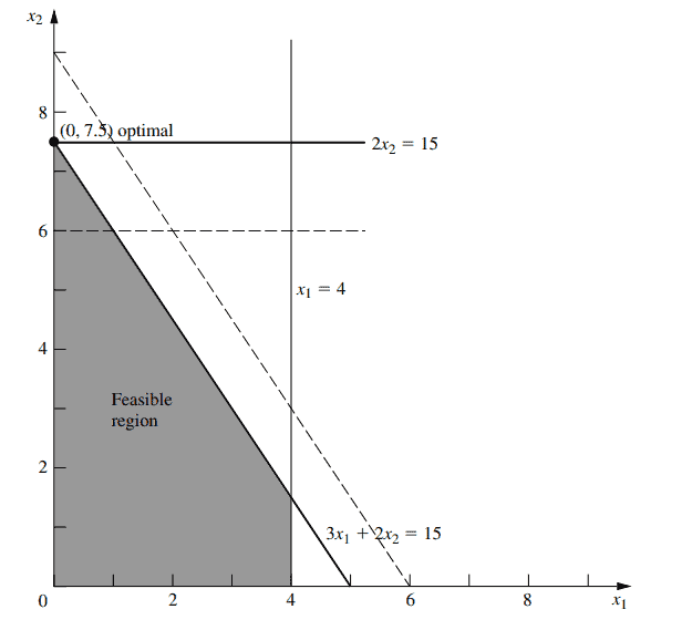
Using Table 6.23 (and referring to Fig. 6.3 for visualization), this 100 percent rule says that $(0,9)$ will remain optimal for Variation 2 of the Wyndor Glass Co. model even if we simultaneously increase $c_1$ from 3 and decrease $c_2$ from 5 as long as these changes are not too large. For example, if $c_1$ is increased by 1.5 (33 $\frac{1}{3}$ percent of the allowable change), then $c_2$ can be decreased by as much as 2 (66 $\frac{2}{2}$ percent of the allowable change). Similarly, if $c_1$ is increased by 3 (66 $\frac{2}{3}$ percent of the allowable change), then $c_2$ can only changes revise the objective function to either $Z=4.5 x_1+3 x_2$ or $Z=6 x_1+4 x_2$, which causes the optimal objective function line in Fig. 6.3 to rotate clockwise until it coincides with the constraint boundary equation $3 x_1+2 x_2=18$.

运筹学代考
数学代写|运筹学作业代写operational research代考|Case 2a—Changes in the Coefficients of a Nonbasic Variable
考虑一个特定的变量$x_j$(固定的$j$),它是最终单纯形表所示的最优解中的一个非基本变量。在情况$2 a$中,当前模型的唯一变化是该变量$-c_j, a_{1 j}, a_{2 j}, \ldots, a_{m j}$ -的一个或多个系数已被更改。因此,让$\bar{c}j$和$\bar{a}{i j}$表示这些参数的新值,用$\overline{\mathbf{A}}j$(矩阵$\overline{\mathbf{A}}$的$j$列)作为包含$\bar{a}{i j}$的向量,我们得到
$$
c_j \longrightarrow \bar{c}_j, \quad \mathbf{A}_j \longrightarrow \overline{\mathbf{A}}_j
$$
修改后的模型。
正如第6.5节开头所描述的,对偶理论提供了一种非常方便的检查这些更改的方法。特别是,如果对偶问题的互补基本解$\mathbf{y}^$仍然满足改变后的单对偶约束,则原始问题的原最优解仍然是最优解。相反,如果$\mathbf{y}^$违反了这个双重约束,那么这个原始解就不再是最优的。
如果最优解发生了变化,而您希望找到新的解,那么您可以很容易地做到这一点。只需应用基本见解来修改最终simplex表中的$x_j$列(唯一更改的列)。具体来说,表6.17中的公式可以简化为:
最后第0行$x_j$系数:
最后1 ~ $m$中$x_j$的系数:
$$
\begin{aligned}
& z_j^-\bar{c}_j=\mathbf{y}^ \overline{\mathbf{A}}_j-\bar{c}_j, \
& \mathbf{A}_j^*=\mathbf{S} * \overline{\mathbf{A}}_j .
\end{aligned}
$$
由于当前基本解不再是最优的,$z_j^*-c_j$的新值现在将是第0行中的一个负系数,因此重新启动单纯形方法,将$x_j$作为初始输入基本变量。
注意,这个过程是第6.6节末尾总结的一般过程的精简版本。步骤3和4(从高斯消去和可行性测试转换为适当形式)已被删除,因为在最终表的修订中(在重新优化之前)唯一更改的列是用于非基本变量$x_j$。第5步(最优性测试)已经被第1步(模型修正)之后执行的更快速的最优性测试所取代。只有当这个测试表明最优解发生了变化,而您希望找到新的解决方案时,才需要第2步和第6步(修改最终表格和重新优化)。
数学代写|运筹学作业代写operational research代考|Analyzing Simultaneous Changes in Objective Function Coefficients
分析目标函数系数的同步变化。无论$x_j$是基本变量还是非基本变量,只有当目标函数系数是唯一被改变的变量时,$c_j$保持最优的允许范围才有效。然而,当目标函数的系数同时发生变化时,可以使用100%规则来检查原始解决方案是否必须仍然是最优的。与右侧同时更改的100%规则非常相似,这个100%规则结合了表(如表6.23)的最后两列给出的单个$c_j$的允许更改(增加或减少),如下所述。
目标函数系数同时变化100%规则:如果目标函数的系数同时发生变化,则计算每次变化允许变化(增加或减少)的百分比,使该系数保持在其允许范围内以保持最佳状态。如果百分比变化的总和不超过100%,那么原始的最优解肯定仍然是最优的。(如果总数确实超过100%,那么我们就不能确定。)
使用表6.23(并参考图6.3进行可视化),这个100%规则表明$(0,9)$对于Wyndor Glass Co.模型的变体2仍然是最优的,即使我们同时从3增加$c_1$并从5减少$c_2$,只要这些变化不是太大。例如,如果$c_1$增加1.5(占允许变化的33% $\frac{1}{3}$ %),那么$c_2$可以减少2(占允许变化的66% $\frac{2}{2}$ %)。同样,如果$c_1$增加3 (66.$\frac{2}{3}$ %的允许变化),则$c_2$只能将目标函数修改为$Z=4.5 x_1+3 x_2$或$Z=6 x_1+4 x_2$,从而导致图6.3中最优目标函数线顺时针旋转,直到与约束边界方程$3 x_1+2 x_2=18$重合。

统计代写请认准statistics-lab™. statistics-lab™为您的留学生涯保驾护航。
金融工程代写
金融工程是使用数学技术来解决金融问题。金融工程使用计算机科学、统计学、经济学和应用数学领域的工具和知识来解决当前的金融问题,以及设计新的和创新的金融产品。
非参数统计代写
非参数统计指的是一种统计方法,其中不假设数据来自于由少数参数决定的规定模型;这种模型的例子包括正态分布模型和线性回归模型。
广义线性模型代考
广义线性模型(GLM)归属统计学领域,是一种应用灵活的线性回归模型。该模型允许因变量的偏差分布有除了正态分布之外的其它分布。
术语 广义线性模型(GLM)通常是指给定连续和/或分类预测因素的连续响应变量的常规线性回归模型。它包括多元线性回归,以及方差分析和方差分析(仅含固定效应)。
有限元方法代写
有限元方法(FEM)是一种流行的方法,用于数值解决工程和数学建模中出现的微分方程。典型的问题领域包括结构分析、传热、流体流动、质量运输和电磁势等传统领域。
有限元是一种通用的数值方法,用于解决两个或三个空间变量的偏微分方程(即一些边界值问题)。为了解决一个问题,有限元将一个大系统细分为更小、更简单的部分,称为有限元。这是通过在空间维度上的特定空间离散化来实现的,它是通过构建对象的网格来实现的:用于求解的数值域,它有有限数量的点。边界值问题的有限元方法表述最终导致一个代数方程组。该方法在域上对未知函数进行逼近。[1] 然后将模拟这些有限元的简单方程组合成一个更大的方程系统,以模拟整个问题。然后,有限元通过变化微积分使相关的误差函数最小化来逼近一个解决方案。
tatistics-lab作为专业的留学生服务机构,多年来已为美国、英国、加拿大、澳洲等留学热门地的学生提供专业的学术服务,包括但不限于Essay代写,Assignment代写,Dissertation代写,Report代写,小组作业代写,Proposal代写,Paper代写,Presentation代写,计算机作业代写,论文修改和润色,网课代做,exam代考等等。写作范围涵盖高中,本科,研究生等海外留学全阶段,辐射金融,经济学,会计学,审计学,管理学等全球99%专业科目。写作团队既有专业英语母语作者,也有海外名校硕博留学生,每位写作老师都拥有过硬的语言能力,专业的学科背景和学术写作经验。我们承诺100%原创,100%专业,100%准时,100%满意。
随机分析代写
随机微积分是数学的一个分支,对随机过程进行操作。它允许为随机过程的积分定义一个关于随机过程的一致的积分理论。这个领域是由日本数学家伊藤清在第二次世界大战期间创建并开始的。
时间序列分析代写
随机过程,是依赖于参数的一组随机变量的全体,参数通常是时间。 随机变量是随机现象的数量表现,其时间序列是一组按照时间发生先后顺序进行排列的数据点序列。通常一组时间序列的时间间隔为一恒定值(如1秒,5分钟,12小时,7天,1年),因此时间序列可以作为离散时间数据进行分析处理。研究时间序列数据的意义在于现实中,往往需要研究某个事物其随时间发展变化的规律。这就需要通过研究该事物过去发展的历史记录,以得到其自身发展的规律。
回归分析代写
多元回归分析渐进(Multiple Regression Analysis Asymptotics)属于计量经济学领域,主要是一种数学上的统计分析方法,可以分析复杂情况下各影响因素的数学关系,在自然科学、社会和经济学等多个领域内应用广泛。
MATLAB代写
MATLAB 是一种用于技术计算的高性能语言。它将计算、可视化和编程集成在一个易于使用的环境中,其中问题和解决方案以熟悉的数学符号表示。典型用途包括:数学和计算算法开发建模、仿真和原型制作数据分析、探索和可视化科学和工程图形应用程序开发,包括图形用户界面构建MATLAB 是一个交互式系统,其基本数据元素是一个不需要维度的数组。这使您可以解决许多技术计算问题,尤其是那些具有矩阵和向量公式的问题,而只需用 C 或 Fortran 等标量非交互式语言编写程序所需的时间的一小部分。MATLAB 名称代表矩阵实验室。MATLAB 最初的编写目的是提供对由 LINPACK 和 EISPACK 项目开发的矩阵软件的轻松访问,这两个项目共同代表了矩阵计算软件的最新技术。MATLAB 经过多年的发展,得到了许多用户的投入。在大学环境中,它是数学、工程和科学入门和高级课程的标准教学工具。在工业领域,MATLAB 是高效研究、开发和分析的首选工具。MATLAB 具有一系列称为工具箱的特定于应用程序的解决方案。对于大多数 MATLAB 用户来说非常重要,工具箱允许您学习和应用专业技术。工具箱是 MATLAB 函数(M 文件)的综合集合,可扩展 MATLAB 环境以解决特定类别的问题。可用工具箱的领域包括信号处理、控制系统、神经网络、模糊逻辑、小波、仿真等。