如果你也在 怎样代写图论Graph Theory 这个学科遇到相关的难题,请随时右上角联系我们的24/7代写客服。图论Graph Theory有趣的部分原因在于,图可以用来对某些问题中的情况进行建模。这些问题可以在图表的帮助下进行研究(并可能得到解决)。因此,图形模型在本书中经常出现。然而,图论是数学的一个领域,因此涉及数学思想的研究-概念和它们之间的联系。我们选择包含的主题和结果是因为我们认为它们有趣、重要和/或代表主题。
There is a simple formula relating the numbers of vertices, edges, and faces in a connected plane graph. It is known as Euler’s Formula because Euler established it for those plane graphs defined by the vertices and edges of polyhedra. In this section, we discuss Euler’s Formula and its immediate consequences.
Theorem 6.3.2 (Euler 1750) Let $G$ be a connected plane graph, and let n, m, and $f$ denote, respectively, the numbers of vertices, edges, and faces of $G$. Then $n-m+f=2$.
Proof We employ an induction on $m$, the result being obvious for $m=0$ or 1 . Assume that $m \geq 2$ and the result is true for all connected plane graphs having fewer than $m$ edges, and suppose that $G$ has $m$ edges. Consider first the case $G$ is a tree. Then $G$ has a vertex $v$ of degree one. The connected plane graph $G-v$ has $n-1$ vertices, $m-1$ edges and $f(=1)$ faces, so by the inductive hypothesis, $(n-1)-(m-1)+f=2$, which implies that $n-m+f=2$. Consider next the case when $G$ is not a tree. Then $G$ has an edge $e$ on a cycle. In this case, the connected plane graph $G-e$ has $n$ vertices, $m-1$ edges, and $f-1$ faces, so that the desired formula immediately follows from the inductive hypothesis.
A maximal planar graph is one to which no edge can be added without losing planarity. Thus in any embedding of a maximal planar graph $G$ with $n \geq 3$, the boundary of every face of $G$ is a triangle, and hence the embedding is often called a triangulated plane graph. Although a general graph may have up to $n(n-1) / 2$ edges, it is not true for planar graphs.
数学代写|图论作业代写Graph Theory代考|Dual Graph
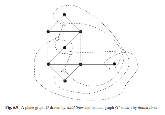
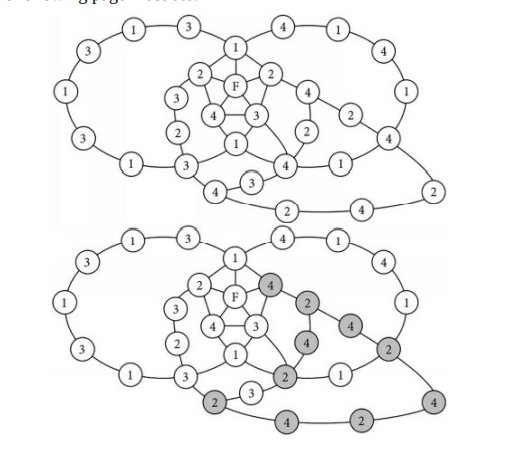
For a plane graph $G$, we often construct another graph $G^$ called the (geometric) dual of $G$ as follows. A vertex $v_i^$ is placed in each face $F_i$ of $G$; these are the vertices of $G^$. Corresponding to each edge $e$ of $G$, we draw an edge $e^$ which crosses $e$ (but no other edge of $G$ ) and joins the vertices $v_i^$ which lie in the faces $F_i$ adjoining $e$; these are the edges of $G^$. The edge $e^$ of $G^$ is called the dual edge of $e$ of $G$. The construction is illustrated in Fig. 6.9; the vertices $v_i^$ are represented by small white circles, and the edges $e^$ of $G^$ by dotted lines. $G^$ is not necessarily a simple graph even if $G$ is simple. Clearly, the dual $G^*$ of a plane graph $G$ is also a plane graph. One can easily observe the following lemma.
Lemma 6.3.6 Let $G$ be a connected plane graph with $n$ vertices, $m$ edges, and $f$ faces, and let the dual $G^$ have $n^$ vertices, $m^$ edges, and $f^$ faces, then $n^=f$, $m^=m$, and $f^*=n$.
Clearly, the dual of the dual of a connected plane graph $G$ is the original graph $G$. However, a planar graph may give rise to two or more geometric duals since the plane embedding is not necessarily unique.
A connected plane graph $G$ is called self-dual if it is isomorphic to its dual $G^$. The graph $G$ in Fig. 6.10 drawn with black vertices and solid edges is a self-dual graph where $G^$ is drawn with white vertices and dotted edges.
A weak dual of a plane graph $G$ is the subgraph of the dual graph of $G$ whose vertices correspond to the inner faces of $G$.
现代博弈论始于约翰-冯-诺伊曼(John von Neumann)提出的两人零和博弈中的混合策略均衡的观点及其证明。冯-诺依曼的原始证明使用了关于连续映射到紧凑凸集的布劳威尔定点定理,这成为博弈论和数学经济学的标准方法。在他的论文之后,1944年,他与奥斯卡-莫根斯特恩(Oskar Morgenstern)共同撰写了《游戏和经济行为理论》一书,该书考虑了几个参与者的合作游戏。这本书的第二版提供了预期效用的公理理论,使数理统计学家和经济学家能够处理不确定性下的决策。
如果你也在 怎样代写图论Graph Theory 这个学科遇到相关的难题,请随时右上角联系我们的24/7代写客服。图论Graph Theory有趣的部分原因在于,图可以用来对某些问题中的情况进行建模。这些问题可以在图表的帮助下进行研究(并可能得到解决)。因此,图形模型在本书中经常出现。然而,图论是数学的一个领域,因此涉及数学思想的研究-概念和它们之间的联系。我们选择包含的主题和结果是因为我们认为它们有趣、重要和/或代表主题。
数学代写|图论作业代写Graph Theory代考|Distances in Trees and Graphs
In this section, we study some distance parameters of graphs and trees. If $G$ has a $u, v$-path, then the distance from $u$ to $v$ is the length of a shortest $u, v$-path. The distance from $u$ to $v$ in $G$ is denoted by $d_G(u, v)$ or simply by $d(u, v)$. For the graph in Fig. 4.10, $d(a, j)=5$ although there is a path of length 8 between $a$ and $j$. If $G$ has no $u, v$-path then $d(u, v)=\infty$. The diameter of $G$ is the longest distance among the distances of all pair of vertices in $G$. The graph in Fig. 4.10 has diameter 6. The eccentricity of a vertex $u$ in $G$ is $\max {v \in V(G)} d(u, v)$ and denoted by $\epsilon(u)$. Eccentricities of all vertices of the graph in Fig. 4.10 are shown in the figure. The radius of a graph is $\min {u \in V(G)} \epsilon(u)$. The center of a graph $G$ is the subgraph of $G$ induced by vertices of minimum ecentricity. The maximum of the vertex eccentricities is equal to the diameter. The radius and the diameter of the graph in Fig. 4.10 is 3 and 6 respectively. The vertex $h$ is the center of the graph in Fig. 4.10. The diameter and the radius of a disconnected graph are infinite.
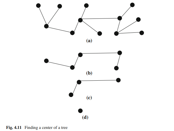
Since there is only one path between any two vertices in a tree, computing the distance parameters for trees is not difficult. We have the following lemma on the center of a tree. Lemma 4.6.1 The center of a tree is a vertex or an edge. Proof We use induction on the number of vertices in a tree $T$. If $n \leq 2$ then the entire tree is the center of the tree. Assume that $n \geq 3$ and the claim holds for any tree with less than $n$ vertices. Let $T^{\prime}$ be the graph obtained from $T$ by deleting all leaves of $T . T^{\prime}$ has at least one vertex, since $T$ has a non-leaf vertex as $n \geq 3$. Clearly $T^{\prime}$ is connected and has no cycle, and hence $T^{\prime}$ be a tree with less than $n$ vertices. By induction hypothesis the center of $T^{\prime}$ is a vertex or an edge. To complete the proof, we now show that $T$ and $T^{\prime}$ have the same center. Let $v$ be a vertex in $T$. Every vertex $u$ in $T$ which is at maximum distance from $v$ is a leaf. Since all leaves of $T$ have been deleted to obtain $T^{\prime}$ and any path between two non-leaf vertices in $T$ does not contain a leaf, $\epsilon_{T^{\prime}}(u)=\epsilon_T(u)-1$ for every vertex $u$ in $T^{\prime}$. Furthermore, the ecentricity of a leaf is greater than the ecentricity of its neighbor in $T$. Hence the In this section, we study some distance parameters of graphs and trees. If $G$ has a $u, v$-path, then the distance from $u$ to $v$ is the length of a shortest $u, v$-path. The distance from $u$ to $v$ in $G$ is denoted by $d_G(u, v)$ or simply by $d(u, v)$. For the graph in Fig. 4.10, $d(a, j)=5$ although there is a path of length 8 between $a$ and $j$. If $G$ has no $u, v$-path then $d(u, v)=\infty$. The diameter of $G$ is the longest distance among the distances of all pair of vertices in $G$. The graph in Fig. 4.10 has diameter 6. The eccentricity of a vertex $u$ in $G$ is $\max {v \in V(G)} d(u, v)$ and denoted by $\epsilon(u)$. Eccentricities of all vertices of the graph in Fig. 4.10 are shown in the figure. The radius of a graph is $\min {u \in V(G)} \epsilon(u)$. The center of a graph $G$ is the subgraph of $G$ induced by vertices of minimum ecentricity. The maximum of the vertex eccentricities is equal to the diameter. The radius and the diameter of the graph in Fig. 4.10 is 3 and 6 respectively. The vertex $h$ is the center of the graph in Fig. 4.10. The diameter and the radius of a disconnected graph are infinite.
Since there is only one path between any two vertices in a tree, computing the distance parameters for trees is not difficult. We have the following lemma on the center of a tree.
数学代写|图论作业代写Graph Theory代考|Graceful Labeling
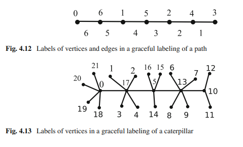
A graceful labeling of a simple graph $G$, with $n$ vertices and $m$ edges, is a one-toone mapping $f$ of the vertex set $V$ into the set ${0,1,2, \ldots, m}$, such that distinct vertices receive distinct numbers and $f$ satisfies ${|f(u)-f(v)|: u v \in E(G)}=$ ${1,2,3, \ldots, m}$. The absolute difference $|f(u)-f(v)|$ is regarded as the label of the edge $e=(u, v)$ in the graceful labeling. The number received by a vertex in a graceful labeling is regarded as the label of the vertex. A graph $G$ is called graceful if $G$ admits a graceful labeling.
One can easily compute a graceful labeling of a path as follows. Start labeling of vertices (i.e., assigning labels to vertices) at either end. The first vertex is labeled by 0 and the next vertex on the path is labeled by $n-1$, the next vertex is labeled by 1 , the next vertex is labeled by $n-2$, and so on. Figure 4.12 illustrates a graceful labeling of a path. It is not difficult to observe that edges get labels $n-1, n-2, \ldots, 1$.
An interesting pattern of labeling exits for a graceful labeling of a “caterpillar.” A caterpillar is a tree for which deletion of all leaves produces a path. Observe Fig. 4.13 for an interesting pattern of graceful labeling of a caterpillar.
All trees are graceful — is the famous Ringel-Kotzig conjecture which has been the focus of many papers. Graphs of different classes have been proven mathematically to be graceful or nongraceful. All trees with 27 vertices are graceful was shown by Aldred and McKay using a computer program in 1998. Aryabhatta et. al showed that a fairly large class of trees constructed from caterpillars are graceful [7]. A lobster is a tree for which deletion of all leaves produces a caterpillar. Morgan showed that a subclass of lobsters are graceful [8].
一个简单图$G$的优美标记,有$n$顶点和$m$边,是顶点集$V$到集合${0,1,2,\ldots, m}$的一对一映射$f$,使得不同的顶点得到不同的数字,并且$f$满足${|f(u)-f(V)|: u V \in E(G)}=$ ${{1,2,3, \ldots, m}$。将绝对差$|f(u)-f(v)|$作为优美标注中边$e=(u, v)$的标注。在优美标记中,一个顶点接收到的数字被视为该顶点的标记。图$G$被称为优美的,如果$G$允许优美的标记。
现代博弈论始于约翰-冯-诺伊曼(John von Neumann)提出的两人零和博弈中的混合策略均衡的观点及其证明。冯-诺依曼的原始证明使用了关于连续映射到紧凑凸集的布劳威尔定点定理,这成为博弈论和数学经济学的标准方法。在他的论文之后,1944年,他与奥斯卡-莫根斯特恩(Oskar Morgenstern)共同撰写了《游戏和经济行为理论》一书,该书考虑了几个参与者的合作游戏。这本书的第二版提供了预期效用的公理理论,使数理统计学家和经济学家能够处理不确定性下的决策。
如果你也在 怎样代写图论Graph Theory 这个学科遇到相关的难题,请随时右上角联系我们的24/7代写客服。图论Graph Theory有趣的部分原因在于,图可以用来对某些问题中的情况进行建模。这些问题可以在图表的帮助下进行研究(并可能得到解决)。因此,图形模型在本书中经常出现。然而,图论是数学的一个领域,因此涉及数学思想的研究-概念和它们之间的联系。我们选择包含的主题和结果是因为我们认为它们有趣、重要和/或代表主题。
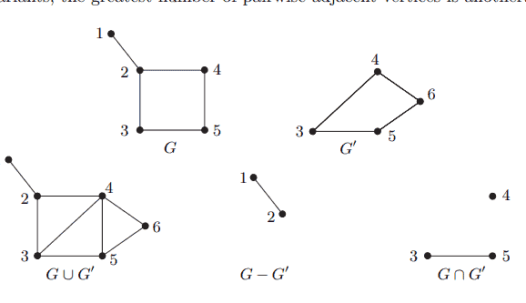
Let $H$ be a graph and $n \geqslant|H|$. How many edges will suffice to force an $H$ subgraph in any graph on $n$ vertices, no matter how these edges are arranged? Or, to rephrase the problem: which is the greatest possible number of edges that a graph on $n$ vertices can have without containing a copy of $H$ as a subgraph? What will such a graph look like? Will it be unique?
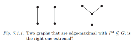
A graph $G \nsupseteq H$ on $n$ vertices with the largest possible number of edges is called extremal for $n$ and $H$; its number of edges is denoted by $\operatorname{ex}(n, H)$. Clearly, any graph $G$ that is extremal for some $n$ and $H$ will also be edge-maximal with $H \nsubseteq G$. Conversely, though, edge-maximality does not imply extremality: $G$ may well be edge-maximal with $H \nsubseteq G$ while having fewer than $\operatorname{ex}(n, H)$ edges (Fig. 7.1.1).
As a case in point, we consider our problem for $H=K^r$ (with $r>1$ ). A moment’s thought suggests some obvious candidates for extremality here: all complete $(r-1)$-partite graphs are edge-maximal without containing $K^r$. But which among these have the greatest number of edges? Clearly those whose partition sets are as equal as possible, i.e. differ in size by at most 1: if $V_1, V_2$ are two partition sets with $\left|V_1\right|-\left|V_2\right| \geqslant 2$, we may increase the number of edges in our complete $(r-1)$-partite graph by moving a vertex from $V_1$ to $V_2$.
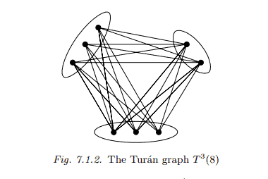
The unique complete $(r-1)$-partite graphs on $n \geqslant r-1$ vertices whose partition sets differ in size by at most 1 are called Turán graphs; we denote them by $T^{r-1}(n)$ and their number of edges by $t_{r-1}(n)$ (Fig. 7.1.2). For $n<r-1$ we shall formally continue to use these definitions, with the proviso that – contrary to our usual terminologythe partition sets may now be empty; then, clearly, $T^{r-1}(n)=K^n$ for all $n \leqslant r-1$.
数学代写|图论作业代写Graph Theory代考|Circulations
In the context of flows, we have to be able to speak about the ‘directions’ of an edge. Since, in a multigraph $G=(V, E)$, an edge $e=x y$ is not identified uniquely by the pair $(x, y)$ or $(y, x)$, we define directed edges as triples: $$ \vec{E}:={(e, x, y) \mid e \in E ; x, y \in V ; e=x y} . $$ Thus, an edge $e=x y$ with $x \neq y$ has the two directions $(e, x, y)$ and $(e, y, x)$; a loop $e=x x$ has only one direction, the triple $(e, x, x)$. For given $\vec{e}=(e, x, y) \in \vec{E}$, we set $\bar{e}:=(e, y, x)$, and for an arbitrary set $\vec{F} \subseteq \vec{E}$ of edge directions we put $$ \bar{F}:={\bar{e} \mid \vec{e} \in \vec{F}} $$ Note that $\vec{E}$ itself is symmetrical: $\bar{E}=\vec{E}$. For $X, Y \subseteq V$ and $\vec{F} \subseteq \vec{E}$, define $$ \vec{F}(X, Y):={(e, x, y) \in \vec{F} \mid x \in X ; y \in Y ; x \neq y}, $$ abbreviate $\vec{F}({x}, Y)$ to $\vec{F}(x, Y)$ etc., and write $$ \vec{F}(x):=\vec{F}(x, V)=\vec{F}({x}, \overline{{x}}) . $$ Here, as below, $\bar{X}$ denotes the complement $V \backslash X$ of a vertex set $X \subseteq V$. Note that any loops at vertices $x \in X \cap Y$ are disregarded in the definitions of $\vec{F}(X, Y)$ and $\vec{F}(x)$.
Let $H$ be an abelian semigroup, ${ }^2$ written additively with zero 0 . Given vertex sets $X, Y \subseteq V$ and a function $f: \vec{E} \rightarrow H$, let $$ f(X, Y):=\sum_{\vec{e} \in \vec{E}(X, Y)} f(\vec{e}) $$
如果你也在 怎样代写图论Graph Theory 这个学科遇到相关的难题,请随时右上角联系我们的24/7代写客服。图论Graph Theory有趣的部分原因在于,图可以用来对某些问题中的情况进行建模。这些问题可以在图表的帮助下进行研究(并可能得到解决)。因此,图形模型在本书中经常出现。然而,图论是数学的一个领域,因此涉及数学思想的研究-概念和它们之间的联系。我们选择包含的主题和结果是因为我们认为它们有趣、重要和/或代表主题。
As discussed in Section 5.2, a high chromatic number may occur as a purely global phenomenon: even when a graph has large girth, and thus locally looks like a tree, its chromatic number may be arbitrarily high. Since such ‘global dependence’ is obviously difficult to deal with, one may become interested in graphs where this phenomenon does not occur, i.e. whose chromatic number is high only when there is a local reason for it. Before we make this precise, let us note two definitions for a graph $G$. The greatest integer $r$ such that $K^r \subseteq G$ is the clique number $\omega(G)$ of $G$, and the greatest integer $r$ such that $\overline{K^r} \subseteq G$ (induced) is the independence number $\alpha(G)$ of $G$. Clearly, $\alpha(G)=\omega(\bar{G})$ and $\omega(G)=\alpha(\bar{G})$. A graph is called perfect if every induced subgraph $H \subseteq G$ has chromatic number $\chi(H)=\omega(H)$, i.e. if the trivial lower bound of $\omega(H)$ colours always suffices to colour the vertices of $H$. Thus, while proving an assertion of the form $\chi(G)>k$ may in general be difficult, even in principle, for a given graph $G$, it can always be done for a perfect graph simply by exhibiting some $K^{k+1}$ subgraph as a ‘certificate’ for non-colourability with $k$ colours.
At first glance, the structure of the class of perfect graphs appears somewhat contrived: although it is closed under induced subgraphs (if only by explicit definition), it is not closed under taking general subgraphs or supergraphs, let alone minors (examples?). However, perfection is an important notion in graph theory: the fact that several fundamental classes of graphs are perfect (as if by fluke) may serve as a superficial indication of this. ${ }^3$
What graphs, then, are perfect? Bipartite graphs are, for instance. Less trivially, the complements of bipartite graphs are perfect, tooa fact equivalent to König’s duality theorem 2.1.1 (Exercise 36). The so-called comparability graphs are perfect, and so are the interval graphs (see the exercises); both these turn up in numerous applications.
In order to study at least one such example in some detail, we prove here that the chordal graphs are perfect: a graph is chordal (or triangulated) if each of its cycles of length at least 4 has a chord, i.e. if it contains no induced cycles other than triangles.
To show that chordal graphs are perfect, we shall first characterize their structure. If $G$ is a graph with induced subgraphs $G_1, G_2$ and $S$, such that $G=G_1 \cup G_2$ and $S=G_1 \cap G_2$, we say that $G$ arises from $G_1$ and $G_2$ by pasting these graphs together along $S$.
数学代写|图论作业代写Graph Theory代考|Circulations
In the context of flows, we have to be able to speak about the ‘directions’ of an edge. Since, in a multigraph $G=(V, E)$, an edge $e=x y$ is not identified uniquely by the pair $(x, y)$ or $(y, x)$, we define directed edges as triples: $$ \vec{E}:={(e, x, y) \mid e \in E ; x, y \in V ; e=x y} . $$ Thus, an edge $e=x y$ with $x \neq y$ has the two directions $(e, x, y)$ and $(e, y, x)$; a loop $e=x x$ has only one direction, the triple $(e, x, x)$. For given $\vec{e}=(e, x, y) \in \vec{E}$, we set $\bar{e}:=(e, y, x)$, and for an arbitrary set $\vec{F} \subseteq \vec{E}$ of edge directions we put $$ \bar{F}:={\bar{e} \mid \vec{e} \in \vec{F}} $$ Note that $\vec{E}$ itself is symmetrical: $\bar{E}=\vec{E}$. For $X, Y \subseteq V$ and $\vec{F} \subseteq \vec{E}$, define $$ \vec{F}(X, Y):={(e, x, y) \in \vec{F} \mid x \in X ; y \in Y ; x \neq y}, $$ abbreviate $\vec{F}({x}, Y)$ to $\vec{F}(x, Y)$ etc., and write $$ \vec{F}(x):=\vec{F}(x, V)=\vec{F}({x}, \overline{{x}}) . $$ Here, as below, $\bar{X}$ denotes the complement $V \backslash X$ of a vertex set $X \subseteq V$. Note that any loops at vertices $x \in X \cap Y$ are disregarded in the definitions of $\vec{F}(X, Y)$ and $\vec{F}(x)$.
Let $H$ be an abelian semigroup, ${ }^2$ written additively with zero 0 . Given vertex sets $X, Y \subseteq V$ and a function $f: \vec{E} \rightarrow H$, let $$ f(X, Y):=\sum_{\vec{e} \in \vec{E}(X, Y)} f(\vec{e}) $$
如果你也在 怎样代写图论Graph Theory 这个学科遇到相关的难题,请随时右上角联系我们的24/7代写客服。图论Graph Theory有趣的部分原因在于,图可以用来对某些问题中的情况进行建模。这些问题可以在图表的帮助下进行研究(并可能得到解决)。因此,图形模型在本书中经常出现。然而,图论是数学的一个领域,因此涉及数学思想的研究-概念和它们之间的联系。我们选择包含的主题和结果是因为我们认为它们有趣、重要和/或代表主题。
An embedding in the plane, or planar embedding, of an (abstract) graph $G$ is an isomorphism between $G$ and a plane graph $H$. The latter will be called a drawing of $G$. We shall not always distinguish notationally between the vertices and edges of $G$ and of $H$. In this section we investigate how two planar embeddings of a graph can differ.
How should we measure the likeness of two embeddings $\rho: G \rightarrow H$ and $\rho^{\prime}: G \rightarrow H^{\prime}$ of a planar graph $G ?$ An obvious way to do this is to consider the canonical isomorphism $\sigma:=\rho^{\prime} \circ \rho^{-1}$ between $H$ and $H^{\prime}$ as abstract graphs, and ask how much of their position in the plane this isomorphism respects or preserves. For example, if $\sigma$ is induced by a simple rotation of the plane, we would hardly consider $\rho$ and $\rho^{\prime}$ as genuinely different ways of drawing $G$.
So let us begin by considering any abstract isomorphism $\sigma: V \rightarrow V^{\prime}$ between two plane graphs $H=(V, E)$ and $H^{\prime}=\left(V^{\prime}, E^{\prime}\right)$, with face sets $F(H)=: F$ and $F\left(H^{\prime}\right)=: F^{\prime}$ say, and try to measure to what degree $\sigma$ respects or preserves the features of $H$ and $H^{\prime}$ as plane graphs. In what follows we shall propose three criteria for this in decreasing order of strictness (and increasing order of ease of handling), and then prove that for most graphs these three criteria turn out to agree. In particular, applied to the isomorphism $\sigma=\rho^{\prime} \circ \rho^{-1}$ considered earlier, all three criteria will say that there is essentially only one way to draw a 3-connected graph.
Our first criterion for measuring how well our abstract isomorphism $\sigma$ preserves the plane features of $H$ and $H^{\prime}$ is perhaps the most natural one. Intuitively, we would like to call $\sigma$ ‘topological’ if it is induced by a homeomorphism from the plane $\mathbb{R}^2$ to itself. To avoid having to grant the outer faces of $H$ and $H^{\prime}$ a special status, however, we take a detour via the homeomorphism $\pi: S^2 \backslash{(0,0,1)} \rightarrow \mathbb{R}^2$ chosen in Section 4.1: we call $\sigma$ a topological isomorphism between the plane graphs $H$ and $H^{\prime}$ if there exists a homeomorphism $\varphi: S^2 \rightarrow S^2$ such that $\psi:=\pi \circ \varphi \circ \pi^{-1}$ induces $\sigma$ on $V \cup E$. (More formally: we ask that $\psi$ agree with $\sigma$ on $V$, and that it map every plane edge $x y \in H$ onto the plane edge $\sigma(x) \sigma(y) \in$ $H^{\prime}$. Unless $\varphi$ fixes the point $(0,0,1)$, the map $\psi$ will be undefined at $\pi\left(\varphi^{-1}(0,0,1)\right)$.)
A graph is called planar if it can be embedded in the plane: if it is isomorphic to a plane graph. A planar graph is maximal, or maximally planar, if it is planar but cannot be extended to a larger planar graph by adding an edge (but no vertex).
Drawings of maximal planar graphs are clearly maximally plane. The converse, however, is not obvious: when we start to draw a planar graph, could it happen that we get stuck half-way with a proper subgraph that is already maximally plane? Our first proposition says that this can never happen, that is, a plane graph is never maximally plane just because it is badly drawn: Proposition 4.4.1. (i) Every maximal plane graph is maximally planar. (ii) A planar graph with $n \geqslant 3$ vertices is maximally planar if and only if it has $3 n-6$ edges. Proof. Apply Proposition 4.2.8 and Corollary 4.2.10.
Which graphs are planar? As we saw in Corollary 4.2.11, no planar graph contains $K^5$ or $K_{3,3}$ as a topological minor. Our aim in this section is to prove the surprising converse, a classic theorem of Kuratowski: any graph without a topological $K^5$ or $K_{3,3}$ minor is planar.
Before we prove Kuratowski’s theorem, let us note that it suffices to consider ordinary minors rather than topological ones:
Lemma 4.4.2. A graph contains $K^5$ or $K_{3,3}$ as a minor if and only if it contains $K^5$ or $K_{3,3}$ as a topological minor.
Proof. By Proposition 1.7.2 it suffices to show that every graph $G$ $(1.7 .2)$ with a $K^5$ minor contains either $K^5$ as a topological minor or $K_{3,3}$ as a minor. So suppose that $G \succcurlyeq K^5$, and let $K \subseteq G$ be minimal such that $K=M K^5$. Then every branch set of $K$ induces a tree in $K$, and between any two branch sets $K$ has exactly one edge. If we take the tree induced by a branch set $V_x$ and add to it the four edges joining it to other branch sets, we obtain another tree, $T_x$ say. By the minimality of $K, T_x$ has exactly 4 leaves, the 4 neighbours of $V_x$ in other branch sets (Fig. 4.4.1).
我们应该如何测量平面图形的两个嵌入$\rho: G \rightarrow H$和$\rho^{\prime}: G \rightarrow H^{\prime}$的相似性$G ?$一个明显的方法是考虑$H$和$H^{\prime}$之间的规范同构$\sigma:=\rho^{\prime} \circ \rho^{-1}$作为抽象图形,并询问它们在平面上的同构尊重或保留了多少位置。例如,如果$\sigma$是由平面的简单旋转引起的,我们几乎不会认为$\rho$和$\rho^{\prime}$是绘制$G$的真正不同的方法。
因此,让我们首先考虑两个平面图形$H=(V, E)$和$H^{\prime}=\left(V^{\prime}, E^{\prime}\right)$之间的抽象同构$\sigma: V \rightarrow V^{\prime}$,比如面集$F(H)=: F$和$F\left(H^{\prime}\right)=: F^{\prime}$,并尝试测量$\sigma$在多大程度上尊重或保留了$H$和$H^{\prime}$作为平面图形的特征。在接下来的内容中,我们将按照严格程度的递减顺序(以及易处理程度的递增顺序)提出三条准则,然后证明对于大多数图,这三条准则是一致的。特别是,应用于前面考虑的同构$\sigma=\rho^{\prime} \circ \rho^{-1}$,所有三个标准都表明,实际上只有一种方法可以绘制3连通图。
Let us return once more to König’s duality theorem for bipartite graphs, Theorem 2.1.1. If we orient every edge of $G$ from $A$ to $B$, the theorem tells us how many disjoint directed paths we need in order to cover all the vertices of $G$ : every directed path has length 0 or 1 , and clearly the number of paths in such a ‘path cover’ is smallest when it contains as many paths of length 1 as possible – in other words, when it contains a maximum-cardinality matching.
In this section we put the above question more generally: how many paths in a given directed graph will suffice to cover its entire vertex set? Of course, this could be asked just as well for undirected graphs. As it turns out, however, the result we shall prove is rather more trivial in the undirected case (exercise), and the directed case will also have an interesting corollary.
A directed path is a directed graph $P \neq \emptyset$ with distinct vertices $x_0, \ldots, x_k$ and edges $e_0, \ldots, e_{k-1}$ such that $e_i$ is an edge directed from $x_i$ to $x_{i+1}$, for all $i<k$. In this section, path will always mean ‘directed path’. The vertex $x_k$ above is the last vertex of the path $P$, and when $\mathcal{P}$ is a set of paths we write $\operatorname{ter}(\mathcal{P})$ for the set of their last vertices. A path cover of a directed graph $G$ is a set of disjoint paths in $G$ which together contain all the vertices of $G$.
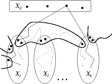
Theorem 2.5.1. (Gallai \& Milgram 1960) Every directed graph $G$ has a path cover $\mathcal{P}$ and an independent set $\left{v_P \mid P \in \mathcal{P}\right}$ of vertices such that $v_P \in P$ for every $P \in \mathcal{P}$.
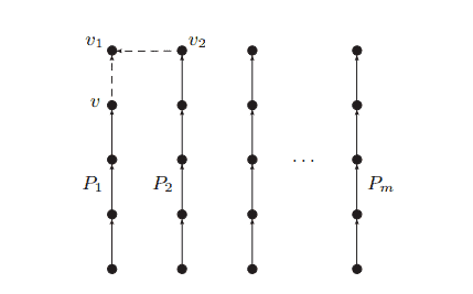
Proof. We prove by induction on $|G|$ that for every path cover $\mathcal{P}=$ $\left{P_1, \ldots, P_m\right}$ of $G$ with $\operatorname{ter}(\mathcal{P})$ minimal there is a set $\left{v_P \mid P \in \mathcal{P}\right}$ as claimed. For each $i$, let $v_i$ denote the last vertex of $P_i$.
If $\operatorname{ter}(\mathcal{P})=\left{v_1, \ldots, v_m\right}$ is independent there is nothing more to show, so we assume that $G$ has an edge from $v_2$ to $v_1$. Since $P_2 v_2 v_1$ is again a path, the minimality of $\operatorname{ter}(\mathcal{P})$ implies that $v_1$ is not the only vertex of $P_1$; let $v$ be the vertex preceding $v_1$ on $P_1$. Then $\mathcal{P}^{\prime}:=$ $\left{P_1 v, P_2, \ldots, P_m\right}$ is a path cover of $G^{\prime}:=G-v_1$ (Fig. 2.5.1). Clearly, any independent set of representatives for $\mathcal{P}^{\prime}$ in $G^{\prime}$ will also work for $\mathcal{P}$ in $G$, so all we have to check is that we may apply the induction hypothesis to $\mathcal{P}^{\prime}$. It thus remains to show that $\operatorname{ter}\left(\mathcal{P}^{\prime}\right)=\left{v, v_2, \ldots, v_m\right}$ is minimal among the sets of last vertices of path covers of $G^{\prime}$.
数学代写|图论作业代写Graph Theory代考|2-Connected graphs and subgraphs
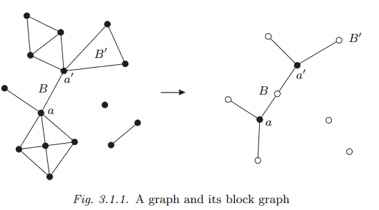
A maximal connected subgraph without a cutvertex is called a block. Thus, every block of a graph $G$ is either a maximal 2-connected subgraph, or a bridge (with its ends), or an isolated vertex. Conversely, every such subgraph is a block. By their maximality, different blocks of $G$ overlap in at most one vertex, which is then a cutvertex of $G$. Hence, every edge of $G$ lies in a unique block, and $G$ is the union of its blocks. Cycles and bonds, too, are confined to a single block:
(i) The cycles of $G$ are precisely the cycles of its blocks. (ii) The bonds of $G$ are precisely the minimal cuts of its blocks. Proof. (i) Any cycle in $G$ is a connected subgraph without a cutvertex, and hence lies in some maximal such subgraph. By definition, this is a block of $G$. (ii) Consider any cut in $G$. Let $x y$ be one of its edges, and $B$ the block containing it. By the maximality of $B$ in the definition of a block, $G$ contains no $B$-path. Hence every $x-y$ path of $G$ lies in $B$, so those edges of our cut that lie in $B$ separate $x$ from $y$ even in $G$. Assertion (ii) follows easily by repeated application of this argument.
In a sense, blocks are the 2-connected analogues of components, the maximal connected subgraphs of a graph. While the structure of $G$ is determined fully by that of its components, however, it is not captured completely by the structure of its blocks: since the blocks need not be disjoint, the way they intersect defines another structure, giving a coarse picture of $G$ as if viewed from a distance.
The following proposition describes this coarse structure of $G$ as formed by its blocks. Let $A$ denote the set of cutvertices of $G$, and $\mathcal{B}$ the set of its blocks. We then have a natural bipartite graph on $A \cup \mathcal{B}$ formed by the edges $a B$ with $a \in B$. This block graph of $G$ is shown in Figure 3.1.1.
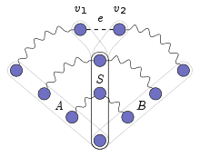
The graphs above are incomplete. These figures only show a vertex with degree four (vertex E), its nearest neighbors (A, B, C, and D), and segments of A-C Kempe chains. The entire graphs would also contain several other vertices (especially, more colored the same as B or D) and enough edges to be MPG’s. The left figure has A connected to $C$ in a single section of an A-C Kempe chain (meaning that the vertices of this chain are colored the same as A and C). The left figure shows that this A-C Kempe chain prevents B from connecting to $\mathrm{D}$ with a single section of a B-D Kempe chain. The middle figure has A and C in separate sections of A-C Kempe chains. In this case, B could connect to D with a single section of a B-D Kempe chain. However, since the A and C of the vertex with degree four lie on separate sections, the color of C’s chain can be reversed so that in the vertex with degree four, C is effectively recolored to match A’s color, as shown in the right figure. Similarly, D’s section could be reversed in the left figure so that D is effectively recolored to match B’s color.
Kempe also attempted to demonstrate that vertices with degree five are fourcolorable in his attempt to prove the four-color theorem [Ref. 2], but his argument for vertices with degree five was shown by Heawood in 1890 to be insufficient [Ref. 3]. Let’s explore what happens if we attempt to apply our reasoning for vertices with degree four to a vertex with degree five.
数学代写|图论作业代写Graph Theory代考|The previous diagrams
The previous diagrams show that when the two color reversals are performed one at a time in the crossed-chain graph, the first color reversal may break the other chain, allowing the second color reversal to affect the colors of one of F’s neighbors. When we performed the $2-4$ reversal to change B from 2 to 4 , this broke the 1-4 chain. When we then performed the 2-3 reversal to change E from 3, this caused C to change from 3 to 2 . As a result, F remains connected to four different colors; this wasn’t reversed to three as expected. Unfortunately, you can’t perform both reversals “at the same time” for the following reason. Let’s attempt to perform both reversals “at the same time.” In this crossed-chain diagram, when we swap 2 and 4 on B’s side of the 1-3 chain, one of the 4’s in the 1-4 chain may change into a 2, and when we swap 2 and 3 on E’s side of the 1-4 chain, one of the 3’s in the 1-3 chain may change into a 2 . This is shown in the following figure: one 2 in each chain is shaded gray. Recall that these figures are incomplete; they focus on one vertex (F), its neighbors (A thru E), and Kempe chains. Other vertices and edges are not shown.
Note how one of the 3’s changed into 2 on the left. This can happen when we reverse $\mathrm{C}$ and $\mathrm{E}$ (which were originally 3 and 2 ) on E’s side of the 1-4 chain. Note also how one of the 4’s changed into 2 on the right. This can happen when we reverse B and D (which were originally 2 and 4) outside of the 1-3 chain. Now we see where a problem can occur when attempting to swap the colors of two chains at the same time. If these two 2’s happen to be connected by an edge like the dashed edge shown above, if we perform the double reversal at the same time, this causes two vertices of the same color to share an edge, which isn’t allowed. We’ll revisit Kempe’s strategy for coloring a vertex with degree five in Chapter $25 .$
数学代写|图论作业代写Graph Theory代考| The shading of one section of the B-R
在上图中,顶点和是四度,因为它连接到其他四个顶点。Kempe 表明顶点 A、B、C 和 D 不能被强制为四种不同的颜色,这样顶点 E 总是可以被着色而不会违反四色定理,无论 MPG 的其余部分看起来如何上一页显示的部分。
A 和 C 或者是 AC Kempe 链的同一部分的一部分,或者它们各自位于 AC Kempe 链的不同部分。(如果一种和C例如,是红色和黄色的,则 AC 链是红黄色链。) – 如果一种和C每个位于 AC Kempe 链的不同部分,其中一个部分的颜色可以反转,这有效地重新着色 C 以匹配 A 的颜色。如果 A 和 C 是 AC Kempe 链的同一部分的一部分,则 B 和 D每个都必须位于 BD Kempe 链的不同部分,因为 AC Kempe 链将阻止任何 BD Kempe 链从 B 到达 D。(如果乙和D是蓝色和绿色,例如,那么一种BD Kempe 链是蓝绿色链。)在这种情况下,由于 B 和 D 分别位于 BD Kempe 链的不同部分,因此 BD Kempe 链的其中一个部分的颜色可以反转,这有效地重新着色 D 以匹配 B颜色。– 因此,可以使 C 与 A 具有相同的颜色或使 D 具有与 A 相同的颜色乙通过反转 Kempe 链的分离部分。
上面的图表是不完整的。这些图只显示了一个四阶顶点(顶点 E)、它的最近邻居(A、B、C 和 D),以及 AC Kempe 链的片段。整个图还将包含几个其他顶点(特别是与 B 或 D 相同的颜色)和足够多的边以成为 MPG。左图有 A 连接到C在 AC Kempe 链的单个部分中(意味着该链的顶点颜色与 A 和 C 相同)。左图显示此 AC Kempe 链阻止 B 连接到DBD Kempe 链条的一个部分。中间的数字在 AC Kempe 链的不同部分有 A 和 C。在这种情况下,B 可以通过 BD Kempe 链的单个部分连接到 D。但是,由于四阶顶点的 A 和 C 位于不同的部分,因此可以反转 C 链的颜色,以便在四阶顶点中,C 有效地重新着色以匹配 A 的颜色,如右图所示. 类似地,可以在左图中反转 D 的部分,以便有效地重新着色 D 以匹配 B 的颜色。
Let $G=(V, E)$ be a graph with $n$ vertices and $m$ edges, say $V=$ $\left{v_1, \ldots, v_n\right}$ and $E=\left{e_1, \ldots, e_m\right}$. The vertex space $\mathcal{V}(G)$ of $G$ is the vector space over the 2-element field $\mathbb{F}_2={0,1}$ of all functions $V \rightarrow \mathbb{F}_2$. Every element of $\mathcal{V}(G)$ corresponds naturally to a subset of $V$, the set of those vertices to which it assigns a 1 , and every subset of $V$ is uniquely represented in $\mathcal{V}(G)$ by its indicator function. We may thus think of $\mathcal{V}(G)$ as the power set of $V$ made into a vector space: the sum $U+U^{\prime}$ of two vertex sets $U, U^{\prime} \subseteq V$ is their symmetric difference (why?), and $U=-U$ for all $U \subseteq V$. The zero in $\mathcal{V}(G)$, viewed in this way, is the empty (vertex) set $\emptyset$. Since $\left{\left{v_1\right}, \ldots,\left{v_n\right}\right}$ is a basis of $\mathcal{V}(G)$, its standard basis, we have $\operatorname{dim} \mathcal{V}(G)=n$.
In the same way as above, the functions $E \rightarrow \mathbb{F}_2$ form the edge space $\mathcal{E}(G)$ of $G$ : its elements are the subsets of $E$, vector addition amounts to symmetric difference, $\emptyset \subseteq E$ is the zero, and $F=-F$ for all $F \subseteq E$. As before, $\left{\left{e_1\right}, \ldots,\left{e_m\right}\right}$ is the standard basis of $\mathcal{E}(G)$, and $\operatorname{dim} \mathcal{E}(G)=m$.
Since the edges of a graph carry its essential structure, we shall mostly be concerned with the edge space. Given two edge sets $F, F^{\prime} \in$ $\mathcal{E}(G)$ and their coefficients $\lambda_1, \ldots, \lambda_m$ and $\lambda_1^{\prime}, \ldots, \lambda_m^{\prime}$ with respect to the standard basis, we write $$ \left\langle F, F^{\prime}\right\rangle:=\lambda_1 \lambda_1^{\prime}+\ldots+\lambda_m \lambda_m^{\prime} \in \mathbb{F}_2 $$ Note that $\left\langle F, F^{\prime}\right\rangle=0$ may hold even when $F=F^{\prime} \neq \emptyset$ : indeed, $\left\langle F, F^{\prime}\right\rangle=0$ if and only if $F$ and $F^{\prime}$ have an even number of edges in common. Given a subspace $\mathcal{F}$ of $\mathcal{E}(G)$, we write $$ \mathcal{F}^{\perp}:={D \in \mathcal{E}(G) \mid\langle F, D\rangle=0 \text { for all } F \in \mathcal{F}} $$ This is again a subspace of $\mathcal{E}(G)$ (the space of all vectors solving a certain set of linear equations-which?), and we have $$ \operatorname{dim} \mathcal{F}+\operatorname{dim} \mathcal{F}^{\perp}=m $$
数学代写|图论作业代写Graph Theory代考|Other notions of graphs
For completeness, we now mention a few other notions of graphs which feature less frequently or not at all in this book.
A hypergraph is a pair $(V, E)$ of disjoint sets, where the elements of $E$ are non-empty subsets (of any cardinality) of $V$. Thus, graphs are special hypergraphs.
A directed graph (or digraph) is a pair $(V, E)$ of disjoint sets (of vertices and edges) together with two maps init: $E \rightarrow V$ and ter: $E \rightarrow V$ assigning to every edge $e$ an initial vertex $\operatorname{init}(e)$ and a terminal vertex ter $(e)$. The edge $e$ is said to be directed from $\operatorname{init}(e)$ to ter $(e)$. Note that a directed graph may have several edges between the same two vertices $x, y$. Such edges are called multiple edges; if they have the same direction (say from $x$ to $y$ ), they are parallel. If init $(e)=\operatorname{ter}(e)$, the edge $e$ is called a $\operatorname{loop}$.
A directed graph $D$ is an orientation of an (undirected) graph $G$ if $V(D)=V(G)$ and $E(D)=E(G)$, and if ${\operatorname{init}(e)$, ter $(e)}={x, y}$ for every edge $e=x y$. Intuitively, such an oriented graph arises from an undirected graph simply by directing every edge from one of its ends to the other. Put differently, oriented graphs are directed graphs without loops or multiple edges.
A multigraph is a pair $(V, E)$ of disjoint sets (of vertices and edges) together with a map $E \rightarrow V \cup[V]^2$ assigning to every edge either one or two vertices, its ends. Thus, multigraphs too can have loops and multiple edges: we may think of a multigraph as a directed graph whose edge directions have been ‘forgotten’. To express that $x$ and $y$ are the ends of an edge $e$ we still write $e=x y$, though this no longer determines $e$ uniquely.
有向图$D$是一个(无向)图$G$的方向,如果$V(D)=V(G)$和$E(D)=E(G)$,如果${\operatorname{init}(e)$, ter $(e)}={x, y}$对于每条边$e=x y$。直观地说,这种有向图是由无向图产生的,只要把每条边从它的一端指向另一端。换句话说,有向图是没有环路或多条边的有向图。
多图是一对$(V, E)$不相交的集合(顶点和边)和一个映射$E \rightarrow V \cup[V]^2$,每个边分配一个或两个顶点,即它的端点。因此,多图也可以有环路和多条边:我们可以认为多图是一个边缘方向被“遗忘”的有向图。为了表示$x$和$y$是边的两端$e$,我们仍然写$e=x y$,尽管这不再唯一地决定$e$。
The graphs above are incomplete. These figures only show a vertex with degree four (vertex E), its nearest neighbors (A, B, C, and D), and segments of A-C Kempe chains. The entire graphs would also contain several other vertices (especially, more colored the same as B or D) and enough edges to be MPG’s. The left figure has A connected to $C$ in a single section of an A-C Kempe chain (meaning that the vertices of this chain are colored the same as A and C). The left figure shows that this A-C Kempe chain prevents B from connecting to $\mathrm{D}$ with a single section of a B-D Kempe chain. The middle figure has A and C in separate sections of A-C Kempe chains. In this case, B could connect to D with a single section of a B-D Kempe chain. However, since the A and C of the vertex with degree four lie on separate sections, the color of C’s chain can be reversed so that in the vertex with degree four, C is effectively recolored to match A’s color, as shown in the right figure. Similarly, D’s section could be reversed in the left figure so that D is effectively recolored to match B’s color.
Kempe also attempted to demonstrate that vertices with degree five are fourcolorable in his attempt to prove the four-color theorem [Ref. 2], but his argument for vertices with degree five was shown by Heawood in 1890 to be insufficient [Ref. 3]. Let’s explore what happens if we attempt to apply our reasoning for vertices with degree four to a vertex with degree five.
数学代写|图论作业代写Graph Theory代考|The previous diagrams
The previous diagrams show that when the two color reversals are performed one at a time in the crossed-chain graph, the first color reversal may break the other chain, allowing the second color reversal to affect the colors of one of F’s neighbors. When we performed the $2-4$ reversal to change B from 2 to 4 , this broke the 1-4 chain. When we then performed the 2-3 reversal to change E from 3, this caused C to change from 3 to 2 . As a result, F remains connected to four different colors; this wasn’t reversed to three as expected. Unfortunately, you can’t perform both reversals “at the same time” for the following reason. Let’s attempt to perform both reversals “at the same time.” In this crossed-chain diagram, when we swap 2 and 4 on B’s side of the 1-3 chain, one of the 4’s in the 1-4 chain may change into a 2, and when we swap 2 and 3 on E’s side of the 1-4 chain, one of the 3’s in the 1-3 chain may change into a 2 . This is shown in the following figure: one 2 in each chain is shaded gray. Recall that these figures are incomplete; they focus on one vertex (F), its neighbors (A thru E), and Kempe chains. Other vertices and edges are not shown.
Note how one of the 3’s changed into 2 on the left. This can happen when we reverse $\mathrm{C}$ and $\mathrm{E}$ (which were originally 3 and 2 ) on E’s side of the 1-4 chain. Note also how one of the 4’s changed into 2 on the right. This can happen when we reverse B and D (which were originally 2 and 4) outside of the 1-3 chain. Now we see where a problem can occur when attempting to swap the colors of two chains at the same time. If these two 2’s happen to be connected by an edge like the dashed edge shown above, if we perform the double reversal at the same time, this causes two vertices of the same color to share an edge, which isn’t allowed. We’ll revisit Kempe’s strategy for coloring a vertex with degree five in Chapter $25 .$
数学代写|图论作业代写Graph Theory代考| The shading of one section of the B-R
在上图中,顶点和是四度,因为它连接到其他四个顶点。Kempe 表明顶点 A、B、C 和 D 不能被强制为四种不同的颜色,这样顶点 E 总是可以被着色而不会违反四色定理,无论 MPG 的其余部分看起来如何上一页显示的部分。
A 和 C 或者是 AC Kempe 链的同一部分的一部分,或者它们各自位于 AC Kempe 链的不同部分。(如果一种和C例如,是红色和黄色的,则 AC 链是红黄色链。) – 如果一种和C每个位于 AC Kempe 链的不同部分,其中一个部分的颜色可以反转,这有效地重新着色 C 以匹配 A 的颜色。如果 A 和 C 是 AC Kempe 链的同一部分的一部分,则 B 和 D每个都必须位于 BD Kempe 链的不同部分,因为 AC Kempe 链将阻止任何 BD Kempe 链从 B 到达 D。(如果乙和D是蓝色和绿色,例如,那么一种BD Kempe 链是蓝绿色链。)在这种情况下,由于 B 和 D 分别位于 BD Kempe 链的不同部分,因此 BD Kempe 链的其中一个部分的颜色可以反转,这有效地重新着色 D 以匹配 B颜色。– 因此,可以使 C 与 A 具有相同的颜色或使 D 具有与 A 相同的颜色乙通过反转 Kempe 链的分离部分。
上面的图表是不完整的。这些图只显示了一个四阶顶点(顶点 E)、它的最近邻居(A、B、C 和 D),以及 AC Kempe 链的片段。整个图还将包含几个其他顶点(特别是与 B 或 D 相同的颜色)和足够多的边以成为 MPG。左图有 A 连接到C在 AC Kempe 链的单个部分中(意味着该链的顶点颜色与 A 和 C 相同)。左图显示此 AC Kempe 链阻止 B 连接到DBD Kempe 链条的一个部分。中间的数字在 AC Kempe 链的不同部分有 A 和 C。在这种情况下,B 可以通过 BD Kempe 链的单个部分连接到 D。但是,由于四阶顶点的 A 和 C 位于不同的部分,因此可以反转 C 链的颜色,以便在四阶顶点中,C 有效地重新着色以匹配 A 的颜色,如右图所示. 类似地,可以在左图中反转 D 的部分,以便有效地重新着色 D 以匹配 B 的颜色。
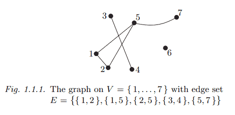
A graph is a pair $G=(V, E)$ of sets such that $E \subseteq[V]^2$; thus, the elements of $E$ are 2-element subsets of $V$. To avoid notational ambiguities, we shall always assume tacitly that $V \cap E=\emptyset$. The elements of $V$ are the vertices (or nodes, or points) of the graph $G$, the elements of $E$ are its edges (or lines). The usual way to picture a graph is by drawing a dot for each vertex and joining two of these dots by a line if the corresponding two vertices form an edge. Just how these dots and lines are drawn is considered irrelevant: all that matters is the information of which pairs of vertices form an edge and which do not.
A graph with vertex set $V$ is said to be a graph on $V$. The vertex set of a graph $G$ is referred to as $V(G)$, its edge set as $E(G)$. These conventions are independent of any actual names of these two sets: the vertex set $W$ of a graph $H=(W, F)$ is still referred to as $V(H)$, not as $W(H)$. We shall not always distinguish strictly between a graph and its vertex or edge set. For example, we may speak of a vertex $v \in G$ (rather than $v \in V(G)$ ), an edge $e \in G$, and so on.
The number of vertices of a graph $G$ is its order, written as $|G|$; its number of edges is denoted by $|G|$. Graphs are finite, infinite, countable and so on according to their order. Except in Chapter 8, our graphs will be finite unless otherwise stated.
For the empty graph $(\emptyset, \emptyset)$ we simply write $\emptyset$. A graph of order 0 or 1 is called trivial. Sometimes, e.g. to start an induction, trivial graphs can be useful; at other times they form silly counterexamples and become a nuisance. To avoid cluttering the text with non-triviality conditions, we shall mostly treat the trivial graphs, and particularly the empty graph $\emptyset$, with generous disregard.
A vertex $v$ is incident with an edge $e$ if $v \in e$; then $e$ is an edge at $v$. The two vertices incident with an edge are its endvertices or ends, and an edge joins its ends. An edge ${x, y}$ is usually written as $x y$ (or $y x$ ). If $x \in X$ and $y \in Y$, then $x y$ is an $X-Y$ edge. The set of all $X-Y$ edges in a set $E$ is denoted by $E(X, Y)$; instead of $E({x}, Y)$ and $E(X,{y})$ we simply write $E(x, Y)$ and $E(X, y)$. The set of all the edges in $E$ at a vertex $v$ is denoted by $E(v)$.
数学代写|图论作业代写Graph Theory代考|The degree of a vertex
Let $G=(V, E)$ be a (non-empty) graph. The set of neighbours of a vertex $v$ in $G$ is denoted by $N_G(v)$, or briefly by $N(v) .^1$ More generally for $U \subseteq V$, the neighbours in $V \backslash U$ of vertices in $U$ are called neighbours of $U$; their set is denoted by $N(U)$.
The degree (or valency) $d_G(v)=d(v)$ of a vertex $v$ is the number $|E(v)|$ of edges at $v$; by our definition of a graph,,$^2$ this is equal to the number of neighbours of $v$. A vertex of degree 0 is isolated. The number $\delta(G):=\min {d(v) \mid v \in V}$ is the minimum degree of $G$, the number $\Delta(G):=\max {d(v) \mid v \in V}$ its maximum degree. If all the vertices of $G$ have the same degree $k$, then $G$ is $k$-regular, or simply regular. A 3 -regular graph is called cubic. The number $$ d(G):=\frac{1}{|V|} \sum_{v \in V} d(v) $$ is the average degree of $G$. Clearly, $$ \delta(G) \leqslant d(G) \leqslant \Delta(G) $$ The average degree quantifies globally what is measured locally by the vertex degrees: the number of edges of $G$ per vertex. Sometimes it will be convenient to express this ratio directly, as $\varepsilon(G):=|E| /|V|$.
The quantities $d$ and $\varepsilon$ are, of course, intimately related. Indeed, if we sum up all the vertex degrees in $G$, we count every edge exactly twice: once from each of its ends. Thus $$ |E|=\frac{1}{2} \sum_{v \in V} d(v)=\frac{1}{2} d(G) \cdot|V|, $$ and therefore $$ \varepsilon(G)=\frac{1}{2} d(G) $$
The graphs above are incomplete. These figures only show a vertex with degree four (vertex E), its nearest neighbors (A, B, C, and D), and segments of A-C Kempe chains. The entire graphs would also contain several other vertices (especially, more colored the same as B or D) and enough edges to be MPG’s. The left figure has A connected to $C$ in a single section of an A-C Kempe chain (meaning that the vertices of this chain are colored the same as A and C). The left figure shows that this A-C Kempe chain prevents B from connecting to $\mathrm{D}$ with a single section of a B-D Kempe chain. The middle figure has A and C in separate sections of A-C Kempe chains. In this case, B could connect to D with a single section of a B-D Kempe chain. However, since the A and C of the vertex with degree four lie on separate sections, the color of C’s chain can be reversed so that in the vertex with degree four, C is effectively recolored to match A’s color, as shown in the right figure. Similarly, D’s section could be reversed in the left figure so that D is effectively recolored to match B’s color.
Kempe also attempted to demonstrate that vertices with degree five are fourcolorable in his attempt to prove the four-color theorem [Ref. 2], but his argument for vertices with degree five was shown by Heawood in 1890 to be insufficient [Ref. 3]. Let’s explore what happens if we attempt to apply our reasoning for vertices with degree four to a vertex with degree five.
数学代写|图论作业代写Graph Theory代考|The previous diagrams
The previous diagrams show that when the two color reversals are performed one at a time in the crossed-chain graph, the first color reversal may break the other chain, allowing the second color reversal to affect the colors of one of F’s neighbors. When we performed the $2-4$ reversal to change B from 2 to 4 , this broke the 1-4 chain. When we then performed the 2-3 reversal to change E from 3, this caused C to change from 3 to 2 . As a result, F remains connected to four different colors; this wasn’t reversed to three as expected. Unfortunately, you can’t perform both reversals “at the same time” for the following reason. Let’s attempt to perform both reversals “at the same time.” In this crossed-chain diagram, when we swap 2 and 4 on B’s side of the 1-3 chain, one of the 4’s in the 1-4 chain may change into a 2, and when we swap 2 and 3 on E’s side of the 1-4 chain, one of the 3’s in the 1-3 chain may change into a 2 . This is shown in the following figure: one 2 in each chain is shaded gray. Recall that these figures are incomplete; they focus on one vertex (F), its neighbors (A thru E), and Kempe chains. Other vertices and edges are not shown.
Note how one of the 3’s changed into 2 on the left. This can happen when we reverse $\mathrm{C}$ and $\mathrm{E}$ (which were originally 3 and 2 ) on E’s side of the 1-4 chain. Note also how one of the 4’s changed into 2 on the right. This can happen when we reverse B and D (which were originally 2 and 4) outside of the 1-3 chain. Now we see where a problem can occur when attempting to swap the colors of two chains at the same time. If these two 2’s happen to be connected by an edge like the dashed edge shown above, if we perform the double reversal at the same time, this causes two vertices of the same color to share an edge, which isn’t allowed. We’ll revisit Kempe’s strategy for coloring a vertex with degree five in Chapter $25 .$
数学代写|图论作业代写Graph Theory代考| The shading of one section of the B-R
在上图中,顶点和是四度,因为它连接到其他四个顶点。Kempe 表明顶点 A、B、C 和 D 不能被强制为四种不同的颜色,这样顶点 E 总是可以被着色而不会违反四色定理,无论 MPG 的其余部分看起来如何上一页显示的部分。
A 和 C 或者是 AC Kempe 链的同一部分的一部分,或者它们各自位于 AC Kempe 链的不同部分。(如果一种和C例如,是红色和黄色的,则 AC 链是红黄色链。) – 如果一种和C每个位于 AC Kempe 链的不同部分,其中一个部分的颜色可以反转,这有效地重新着色 C 以匹配 A 的颜色。如果 A 和 C 是 AC Kempe 链的同一部分的一部分,则 B 和 D每个都必须位于 BD Kempe 链的不同部分,因为 AC Kempe 链将阻止任何 BD Kempe 链从 B 到达 D。(如果乙和D是蓝色和绿色,例如,那么一种BD Kempe 链是蓝绿色链。)在这种情况下,由于 B 和 D 分别位于 BD Kempe 链的不同部分,因此 BD Kempe 链的其中一个部分的颜色可以反转,这有效地重新着色 D 以匹配 B颜色。– 因此,可以使 C 与 A 具有相同的颜色或使 D 具有与 A 相同的颜色乙通过反转 Kempe 链的分离部分。
上面的图表是不完整的。这些图只显示了一个四阶顶点(顶点 E)、它的最近邻居(A、B、C 和 D),以及 AC Kempe 链的片段。整个图还将包含几个其他顶点(特别是与 B 或 D 相同的颜色)和足够多的边以成为 MPG。左图有 A 连接到C在 AC Kempe 链的单个部分中(意味着该链的顶点颜色与 A 和 C 相同)。左图显示此 AC Kempe 链阻止 B 连接到DBD Kempe 链条的一个部分。中间的数字在 AC Kempe 链的不同部分有 A 和 C。在这种情况下,B 可以通过 BD Kempe 链的单个部分连接到 D。但是,由于四阶顶点的 A 和 C 位于不同的部分,因此可以反转 C 链的颜色,以便在四阶顶点中,C 有效地重新着色以匹配 A 的颜色,如右图所示. 类似地,可以在左图中反转 D 的部分,以便有效地重新着色 D 以匹配 B 的颜色。
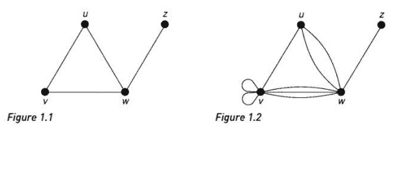
A simple graph $G$ consists of a non-empty finite set $V(G)$ of elements called vertices (or nodes or points) and a finite set $E(G)$ of distinct unordered pairs of distinct elements of $V(G)$ called edges (or lines). We call $V(G)$ the vertex-set and $E(G)$ the edge-set of $G$. An edge ${v, w}$ is said to join the vertices $v$ and $w$, and is usually abbreviated to $v w$. For example, Fig. 1.1 represents the simple graph $G$ whose vertex-set $V(G)$ is ${u, v, w, z}$, and whose edge-set $E(G)$ consists of the edges $u v, u w, v w$ and $w z$. In any simple graph there is at most one edge joining a given pair of vertices. However, many results for simple graphs also hold for more general objects in which two vertices may have several edges joining them; such edges are called multiple edges. In addition, we may remove the restriction that an edge must join two distinct vertices, and allow loops – edges joining a vertex to itself. The resulting object, with loops and multiple edges allowed, is called a general graph – or, simply, a graph (see Fig. 1.2). Note that every simple graph is a graph, but not every graph is a simple graph.
Thus, a graph $G$ consists of a non-empty finite set $V(G)$ of elements called vertices and a finite family $E(G)$ of unordered pairs of (not necessarily distinct) elements of $V(G)$ called edges; the use of the word ‘family’ permits the existence of multiple edges. We call $V(G)$ the vertex-set and $E(G)$ the edge-family of $G$. An edge ${v, w}$ is said to join the vertices $v$ and $w$, and is again abbreviated to $v w$. Thus in Fig. 1.2, $V(G)$ is the set ${u, v, w, z}$ and $E(G)$ consists of the edges $u v, v v$ (twice), $v w$ (three times), $u w$ (twice) and $w z$. Note that each loop $v v$ joins the vertex $v$ to itself. Although we sometimes need to restrict our attention to simple graphs, we shall prove our results for general graphs whenever possible.
Remark. The language of graph theory is not standard – all authors have their own terminology. Some use the term ‘graph’ for what we call a simple graph, while others use it for graphs with directed edges, or for graphs with infinitely many vertices or edges; we discuss these variations in Section 1.3. Any such definition is perfectly valid, provided that it is used consistently. In this book:
All graphs are finite and undirected, with loops and multiple edges allowed unless specifically excluded.
数学代写|图论作业代写Graph Theory代考|Examples
In this section we examine some important types of graphs. You should become familiar with them, as they will appear frequently in examples and exercises. Null graphs A graph whose edge-set is empty is a null graph; note that each vertex of a null graph is isolated. We denote the null graph on $n$ vertices by $N_n$ : the graph $N_4$ is shown in Fig. 1.31. Null graphs are not very interesting.
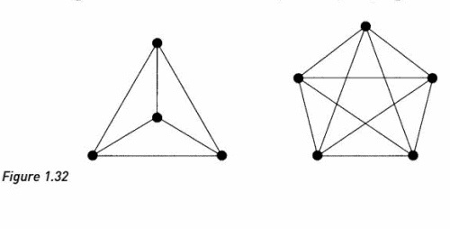
Complete graphs A simple graph in which each pair of distinct vertices are adjacent is a complete graph. We denote the complete graph on $n$ vertices by $K_{r r}$ the graphs $K_4$ and $K_5$ are shown in Fig. 1.32. You should check that $K_n$ has $1 / 2 n(n-1)$ edges.
Cycle graphs, path graphs and wheels A connected graph in which each vertex has degree 2 is a cycle graph. We denote the cycle graph on $n$ vertices by $C_r$
The graph obtained from $C_n$ by removing an edge is the path graph on $n$ vertices, denoted by $P_{n r}$
The graph obtained from $C_{n-1}$ by joining each vertex to a new vertex $v$ is the wheel on $n$ vertices, denoted by $W_{r r}$ The graphs $C_6, P_6$ and $W_6$ are shown in Fig. 1.33.
The graphs above are incomplete. These figures only show a vertex with degree four (vertex E), its nearest neighbors (A, B, C, and D), and segments of A-C Kempe chains. The entire graphs would also contain several other vertices (especially, more colored the same as B or D) and enough edges to be MPG’s. The left figure has A connected to $C$ in a single section of an A-C Kempe chain (meaning that the vertices of this chain are colored the same as A and C). The left figure shows that this A-C Kempe chain prevents B from connecting to $\mathrm{D}$ with a single section of a B-D Kempe chain. The middle figure has A and C in separate sections of A-C Kempe chains. In this case, B could connect to D with a single section of a B-D Kempe chain. However, since the A and C of the vertex with degree four lie on separate sections, the color of C’s chain can be reversed so that in the vertex with degree four, C is effectively recolored to match A’s color, as shown in the right figure. Similarly, D’s section could be reversed in the left figure so that D is effectively recolored to match B’s color.
Kempe also attempted to demonstrate that vertices with degree five are fourcolorable in his attempt to prove the four-color theorem [Ref. 2], but his argument for vertices with degree five was shown by Heawood in 1890 to be insufficient [Ref. 3]. Let’s explore what happens if we attempt to apply our reasoning for vertices with degree four to a vertex with degree five.
数学代写|图论作业代写Graph Theory代考|The previous diagrams
The previous diagrams show that when the two color reversals are performed one at a time in the crossed-chain graph, the first color reversal may break the other chain, allowing the second color reversal to affect the colors of one of F’s neighbors. When we performed the $2-4$ reversal to change B from 2 to 4 , this broke the 1-4 chain. When we then performed the 2-3 reversal to change E from 3, this caused C to change from 3 to 2 . As a result, F remains connected to four different colors; this wasn’t reversed to three as expected. Unfortunately, you can’t perform both reversals “at the same time” for the following reason. Let’s attempt to perform both reversals “at the same time.” In this crossed-chain diagram, when we swap 2 and 4 on B’s side of the 1-3 chain, one of the 4’s in the 1-4 chain may change into a 2, and when we swap 2 and 3 on E’s side of the 1-4 chain, one of the 3’s in the 1-3 chain may change into a 2 . This is shown in the following figure: one 2 in each chain is shaded gray. Recall that these figures are incomplete; they focus on one vertex (F), its neighbors (A thru E), and Kempe chains. Other vertices and edges are not shown.
Note how one of the 3’s changed into 2 on the left. This can happen when we reverse $\mathrm{C}$ and $\mathrm{E}$ (which were originally 3 and 2 ) on E’s side of the 1-4 chain. Note also how one of the 4’s changed into 2 on the right. This can happen when we reverse B and D (which were originally 2 and 4) outside of the 1-3 chain. Now we see where a problem can occur when attempting to swap the colors of two chains at the same time. If these two 2’s happen to be connected by an edge like the dashed edge shown above, if we perform the double reversal at the same time, this causes two vertices of the same color to share an edge, which isn’t allowed. We’ll revisit Kempe’s strategy for coloring a vertex with degree five in Chapter $25 .$
数学代写|图论作业代写Graph Theory代考| The shading of one section of the B-R
在上图中,顶点和是四度,因为它连接到其他四个顶点。Kempe 表明顶点 A、B、C 和 D 不能被强制为四种不同的颜色,这样顶点 E 总是可以被着色而不会违反四色定理,无论 MPG 的其余部分看起来如何上一页显示的部分。
A 和 C 或者是 AC Kempe 链的同一部分的一部分,或者它们各自位于 AC Kempe 链的不同部分。(如果一种和C例如,是红色和黄色的,则 AC 链是红黄色链。) – 如果一种和C每个位于 AC Kempe 链的不同部分,其中一个部分的颜色可以反转,这有效地重新着色 C 以匹配 A 的颜色。如果 A 和 C 是 AC Kempe 链的同一部分的一部分,则 B 和 D每个都必须位于 BD Kempe 链的不同部分,因为 AC Kempe 链将阻止任何 BD Kempe 链从 B 到达 D。(如果乙和D是蓝色和绿色,例如,那么一种BD Kempe 链是蓝绿色链。)在这种情况下,由于 B 和 D 分别位于 BD Kempe 链的不同部分,因此 BD Kempe 链的其中一个部分的颜色可以反转,这有效地重新着色 D 以匹配 B颜色。– 因此,可以使 C 与 A 具有相同的颜色或使 D 具有与 A 相同的颜色乙通过反转 Kempe 链的分离部分。
上面的图表是不完整的。这些图只显示了一个四阶顶点(顶点 E)、它的最近邻居(A、B、C 和 D),以及 AC Kempe 链的片段。整个图还将包含几个其他顶点(特别是与 B 或 D 相同的颜色)和足够多的边以成为 MPG。左图有 A 连接到C在 AC Kempe 链的单个部分中(意味着该链的顶点颜色与 A 和 C 相同)。左图显示此 AC Kempe 链阻止 B 连接到DBD Kempe 链条的一个部分。中间的数字在 AC Kempe 链的不同部分有 A 和 C。在这种情况下,B 可以通过 BD Kempe 链的单个部分连接到 D。但是,由于四阶顶点的 A 和 C 位于不同的部分,因此可以反转 C 链的颜色,以便在四阶顶点中,C 有效地重新着色以匹配 A 的颜色,如右图所示. 类似地,可以在左图中反转 D 的部分,以便有效地重新着色 D 以匹配 B 的颜色。
Many of the sets that are dealt with in graph theory are finite. As for familiar infinite sets, we write $\mathbf{Z}$ for the set of integers, $\mathbf{N}$ for the set of positive integers (natural numbers), $\mathbf{Q}$ for the set of rational numbers and $\mathbf{R}$ for the set of real numbers. Among the infinite sets, we are, by far, most interested in the integers. Even when dealing with a rational number or real number, we are often concerned with a nearby integer. For a real number $x$, the floor $\lfloor x\rfloor$ of $x$ is the greatest integer less than or equal to $x$. So, for example, $\lfloor 5\rfloor=5,\lfloor\sqrt{2}\rfloor=1,\lfloor\pi\rfloor=3$ and $$ \left\lfloor\frac{7+\sqrt{1+96}}{2}\right\rfloor=8 \text {. } $$ The ceiling $\lceil x\rceil$ of $x$ is the smallest integer greater than or equal to $x$. For example, $\lceil 5\rceil=5,\lceil\sqrt{2}\rceil=2,\lceil$ $\pi\rceil 4$ and $$ \left\lceil\frac{(8-3)(8-4)}{12}\right\rceil=2 . $$ For a finite set $S$, we denote its cardinality (the number of elements in $S$ ) by $|S|$. If $|S|=n$ for some $n \in \mathbf{N}$, then we can write $S=\left{s_1, s_2, \ldots, s_n\right}$. The set with cardinality 0 is the empty set, which is denoted by $ø$. Thus $\varnothing={}$. For two sets $A$ and $B$, the Cartesian product $A \times B$ of $A$ and $B$ is the set $$ A \times B={(a, b): a \in A, b \in B} $$
数学代写|图论作业代写Graph Theory代考|Logic
A statement $P$ is a declarative sentence that is true or false but not both. If $P$ is a true statement, then its truth value is true; otherwise, its truth value is false. The negation $\sim P($ not $P$ ) of $P$ has the opposite truth value of $P$. The disjunction $P \vee Q(P$ or $Q)$ of two statements $P$ and $Q$ is true if at least one of $P$ and $Q$ is true and is false otherwise. The conjunction $P \wedge Q(P$ and $Q)$ of $P$ and $Q$ is true if both $P$ and $Q$ are true and is false otherwise. Two statements constructed from $P$ and $Q$ and logical connectives (such as $\sim, V$ and $\Lambda$ ) are logically equivalent if they have the same truth values for all possible combinations of truth values for $P$ and $Q$. According to De Morgan’s laws, for statements $P$ and $Q$, $\sim(P \vee Q)$ is logically equivalent to $(\sim P) \wedge(\sim Q)$ and $\sim(P \wedge Q)$ is logically equivalent to $(\sim P) \vee(\sim Q)$. For statements $P$ and $Q$, the implication $P \Rightarrow Q$ often expressed as “If $P$, then Q.” is true for all combinations of truth values $P$ and $Q$ except when $P$ is true and $Q$ is false. Other ways to express $P$ $\Rightarrow Q$ in words are: (1) $P$ implies $Q$; (2) $P$ only if $Q$; (3) $P$ is sufficient for $Q$; (4) $Q$ is necessary for $P$. In this case, $P$ is a sufficient condition for $Q$ and $Q$ is a necessary condition for $P$.
A declarative sentence containing one or more variables is often referred to as an open sentence. When the variables are assigned values (from some prescribed set or sets), the open sentence is converted into a statement whose truth value depends on the values assigned to the variables. An open sentence expressed in terms of a real number variable $x$ might be denoted by $P(x)$ or $Q(x)$. Since $P(x)$ and $Q(x)$ are open sentences and not statements, they do not have truth values. Similarly $P(x), P(x) \vee$ $Q(x), P(x) \wedge Q(x)$ and $P(x) \Rightarrow Q(x)$ are then also open sentences, not statements. While $$ P(x): 2 x^2+x-1=0 $$ is an open sentence with a real number variable $x$, assigning $x$ the values -1 and $1 / 2$ produces the statements $$ P(1): 2(-1)^2+(-1)-1=0 \text { and } P\left(\frac{1}{2}\right): 2\left(\frac{1}{2}\right)^2+\left(\frac{1}{2}\right)-1=0 \text {, } $$ both of which are true. For every real number $r \neq-1, \frac{1}{2}$, however, $P(r)$ is a false statement.
The graphs above are incomplete. These figures only show a vertex with degree four (vertex E), its nearest neighbors (A, B, C, and D), and segments of A-C Kempe chains. The entire graphs would also contain several other vertices (especially, more colored the same as B or D) and enough edges to be MPG’s. The left figure has A connected to $C$ in a single section of an A-C Kempe chain (meaning that the vertices of this chain are colored the same as A and C). The left figure shows that this A-C Kempe chain prevents B from connecting to $\mathrm{D}$ with a single section of a B-D Kempe chain. The middle figure has A and C in separate sections of A-C Kempe chains. In this case, B could connect to D with a single section of a B-D Kempe chain. However, since the A and C of the vertex with degree four lie on separate sections, the color of C’s chain can be reversed so that in the vertex with degree four, C is effectively recolored to match A’s color, as shown in the right figure. Similarly, D’s section could be reversed in the left figure so that D is effectively recolored to match B’s color.
Kempe also attempted to demonstrate that vertices with degree five are fourcolorable in his attempt to prove the four-color theorem [Ref. 2], but his argument for vertices with degree five was shown by Heawood in 1890 to be insufficient [Ref. 3]. Let’s explore what happens if we attempt to apply our reasoning for vertices with degree four to a vertex with degree five.
数学代写|图论作业代写Graph Theory代考|The previous diagrams
The previous diagrams show that when the two color reversals are performed one at a time in the crossed-chain graph, the first color reversal may break the other chain, allowing the second color reversal to affect the colors of one of F’s neighbors. When we performed the $2-4$ reversal to change B from 2 to 4 , this broke the 1-4 chain. When we then performed the 2-3 reversal to change E from 3, this caused C to change from 3 to 2 . As a result, F remains connected to four different colors; this wasn’t reversed to three as expected. Unfortunately, you can’t perform both reversals “at the same time” for the following reason. Let’s attempt to perform both reversals “at the same time.” In this crossed-chain diagram, when we swap 2 and 4 on B’s side of the 1-3 chain, one of the 4’s in the 1-4 chain may change into a 2, and when we swap 2 and 3 on E’s side of the 1-4 chain, one of the 3’s in the 1-3 chain may change into a 2 . This is shown in the following figure: one 2 in each chain is shaded gray. Recall that these figures are incomplete; they focus on one vertex (F), its neighbors (A thru E), and Kempe chains. Other vertices and edges are not shown.
Note how one of the 3’s changed into 2 on the left. This can happen when we reverse $\mathrm{C}$ and $\mathrm{E}$ (which were originally 3 and 2 ) on E’s side of the 1-4 chain. Note also how one of the 4’s changed into 2 on the right. This can happen when we reverse B and D (which were originally 2 and 4) outside of the 1-3 chain. Now we see where a problem can occur when attempting to swap the colors of two chains at the same time. If these two 2’s happen to be connected by an edge like the dashed edge shown above, if we perform the double reversal at the same time, this causes two vertices of the same color to share an edge, which isn’t allowed. We’ll revisit Kempe’s strategy for coloring a vertex with degree five in Chapter $25 .$
数学代写|图论作业代写Graph Theory代考| The shading of one section of the B-R
在上图中,顶点和是四度,因为它连接到其他四个顶点。Kempe 表明顶点 A、B、C 和 D 不能被强制为四种不同的颜色,这样顶点 E 总是可以被着色而不会违反四色定理,无论 MPG 的其余部分看起来如何上一页显示的部分。
A 和 C 或者是 AC Kempe 链的同一部分的一部分,或者它们各自位于 AC Kempe 链的不同部分。(如果一种和C例如,是红色和黄色的,则 AC 链是红黄色链。) – 如果一种和C每个位于 AC Kempe 链的不同部分,其中一个部分的颜色可以反转,这有效地重新着色 C 以匹配 A 的颜色。如果 A 和 C 是 AC Kempe 链的同一部分的一部分,则 B 和 D每个都必须位于 BD Kempe 链的不同部分,因为 AC Kempe 链将阻止任何 BD Kempe 链从 B 到达 D。(如果乙和D是蓝色和绿色,例如,那么一种BD Kempe 链是蓝绿色链。)在这种情况下,由于 B 和 D 分别位于 BD Kempe 链的不同部分,因此 BD Kempe 链的其中一个部分的颜色可以反转,这有效地重新着色 D 以匹配 B颜色。– 因此,可以使 C 与 A 具有相同的颜色或使 D 具有与 A 相同的颜色乙通过反转 Kempe 链的分离部分。
上面的图表是不完整的。这些图只显示了一个四阶顶点(顶点 E)、它的最近邻居(A、B、C 和 D),以及 AC Kempe 链的片段。整个图还将包含几个其他顶点(特别是与 B 或 D 相同的颜色)和足够多的边以成为 MPG。左图有 A 连接到C在 AC Kempe 链的单个部分中(意味着该链的顶点颜色与 A 和 C 相同)。左图显示此 AC Kempe 链阻止 B 连接到DBD Kempe 链条的一个部分。中间的数字在 AC Kempe 链的不同部分有 A 和 C。在这种情况下,B 可以通过 BD Kempe 链的单个部分连接到 D。但是,由于四阶顶点的 A 和 C 位于不同的部分,因此可以反转 C 链的颜色,以便在四阶顶点中,C 有效地重新着色以匹配 A 的颜色,如右图所示. 类似地,可以在左图中反转 D 的部分,以便有效地重新着色 D 以匹配 B 的颜色。