如果你也在 怎样代写数据科学data science这个学科遇到相关的难题,请随时右上角联系我们的24/7代写客服。
数据科学是一个跨学科领域,它使用科学方法、流程、算法和系统从嘈杂的、结构化和非结构化的数据中提取知识和见解,并在广泛的应用领域应用数据的知识和可操作的见解。
statistics-lab™ 为您的留学生涯保驾护航 在代写数据科学data science方面已经树立了自己的口碑, 保证靠谱, 高质且原创的统计Statistics代写服务。我们的专家在代写数据科学data science方面经验极为丰富,各种代写数据科学data science相关的作业也就用不着说。
我们提供的数据科学data science及其相关学科的代写,服务范围广, 其中包括但不限于:
- Statistical Inference 统计推断
- Statistical Computing 统计计算
- Advanced Probability Theory 高等楖率论
- Advanced Mathematical Statistics 高等数理统计学
- (Generalized) Linear Models 广义线性模型
- Statistical Machine Learning 统计机器学习
- Longitudinal Data Analysis 纵向数据分析
- Foundations of Data Science 数据科学基础

统计代写|数据科学代写data science代考|Principal Component Analysis
PCA is a data analysis technique that relies on a simple transformation of recorded observation, stored in a vector $\mathbf{z} \in \mathbb{R}^{N}$, to produce statistically independent score variables, stored in $\mathrm{t} \in \mathbb{R}^{n}, n \leq N$ :
$$
\mathrm{t}=\mathbf{P}^{T} \mathbf{z}
$$
Here, $\mathbf{P}$ is a transformation matrix, constructed from orthonormal column vectors. Since the first applications of $\mathrm{PCA}[21]$, this technique has found its way into a wide range of different application areas, for example signal processing $[75]$, factor analysis $[29,44]$, system identification $[77]$, chemometrics $[20,66]$ and more recently, general data mining $[11,58,70]$ including image processing $[17,72]$ and pattern recognition $[10,47]$, as well as process monitoring and quality control $[1,82]$ including multiway [48], multiblock [52] and
multiscale [3] extensions. This success is mainly related to the ability of PCA to describe significant information/variation within the recorded data typically by the first few score variables, which simplifies data analysis tasks accordingly.
Sylvester $[67]$ formulated the idea behind PCA, in his work the removal of redundancy in bilinear quantics, that are polynomial expressions where the sum of the exponents are of an order greater than 2, and Pearson [51] laid the conceptual basis for PCA by defining lines and planes in a multivariable space that present the closest fit to a given set of points. Hotelling [28] then refined this formulation to that used today. Numerically, PCA is closely related to an eigenvector-eigenvalue decomposition of a data covariance, or correlation matrix and numerical algorithms to obtain this decomposition include the iterative NIPALS algorithm [78], which was defined similarly by Fisher and MacKenzie earlier in $[80]$, and the singular value decomposition. Good overviews concerning $\mathrm{PCA}$ are given in Mardia et al. [45], Joliffe [32]. Wold et al. $[80]$ and Jackson [30].
‘The aim of this article is to review and examine nonlinear extensions of PCA that have been proposed over the past two decades. This is an important research field, as the application of linear PCA to nonlinear data may be inadequate [49]. The first attempts to present nonlinear PCA extensions include a generalization, utilizing a nonmetric scaling, that produces a nonlinear optimization problem [42] and constructing a curves through a given cloud of points, referred to as principal curves [25]. Inspired by the fact that the reconstruction of the original variables, $\widehat{\mathbf{z}}$ is given by:
$$
\widehat{\mathbf{z}}=\mathbf{P t}=\overbrace{\mathbf{P} \underbrace{\left(\mathbf{P}^{T} \mathbf{z}\right)}_{\text {mapping }}}^{\text {demapping }},
$$
that includes the determination of the score variables (mapping stage) and the determination of $\widehat{\mathbf{z}}$ (demapping stage), Kramer [37] proposed an autoassociative neural network (ANN) structure that defines the mapping and demapping stages by neural network layers. Tan and Mavrovouniotis [68] pointed out, however, that the 5 layers network topology of autoassociative neural networks may be difficult to train, i.e. network weights are difficult to determine if the number of layers increases [27].
To reduce the network complexity, Tan and Mavrovouniotis proposed an input training (IT) network topology, which omits the mapping layer. Thus, only a 3 layer network remains, where the reduced set of nonlinear principal components are obtained as part of the training procedure for establishing the IT network. Dong and McAvoy [16] introduced an alternative approach that divides the 5 layer autoassociative network topology into two 3 layer topologies, which, in turn, represent the nonlinear mapping and demapping functions. The output of the first network, that is the mapping layer, are the score variables which are determined using the principal curve approach.
统计代写|数据科学代写data science代考|PCA Preliminaries
where $N$ and $K$ are the number of recorded variables and the number of available observations, respectively. Defining the rows and columns of $\mathbf{Z}$ by vectors $\mathbf{z}{i} \in \mathbb{R}^{N}$ and $\zeta{j} \in \mathbb{R}^{K}$, respectively, $\mathbf{Z}$ can be rewritten as shown below:
$$
\mathbf{Z}=\left[\begin{array}{c}
\mathbf{z}{1}^{T} \ \mathbf{z}{2}^{T} \
\mathbf{z}{3}^{T} \ \vdots \ \mathbf{z}{i}^{T} \
\vdots \
\mathbf{z}{K-1}^{T} \ \mathbf{z}{K}^{T}
\end{array}\right]=\left[\begin{array}{lll}
\boldsymbol{\zeta}{1} \ \boldsymbol{\zeta}{2}
\end{array} \boldsymbol{\zeta}{3} \cdots \boldsymbol{\zeta}{j} \cdots \boldsymbol{\zeta}{N}\right] $$ The first and second order statisties of the original set variables $\mathbf{z}^{T}=$ $\left(z{1} z_{2} z_{3} \cdots z_{j} \cdots z_{N}\right)$ are:
$$
E{\mathbf{z}}=\mathbf{0} \quad E\left{\mathbf{z z}^{T}\right}=\mathbf{S}{Z Z} $$ with the correlation matrix of $\mathbf{z}$ being defined as $\mathbf{R}{Z Z}$.
The PCA analysis entails the determination of a set of score variables $t_{k}, k \in{123 \cdots n}, n \leq N$, by applying a linear transformation of $\mathbf{z}$ :
$$
t_{k}=\sum_{j=1}^{N} p_{k j} z_{j}
$$
under the following constraint for the parameter vector
$$
\begin{gathered}
\mathbf{p}{k}^{T}=\left(p{k 1} p_{k 2} p_{k 3} \cdots p_{k j} \cdots p_{k}\right. \
\sqrt{\sum_{j=1}^{N} p_{k j}^{2}}=\left|\mathbf{p}{k}\right|{2}=1 .
\end{gathered}
$$
Storing the score variables in a vector $\mathbf{t}^{T}=\left(t_{1} t_{2} t_{3} \cdots t_{j} \cdots t_{n}\right), \mathbf{t} \in \mathbb{R}^{n}$ has the following first and second order statistics:
$$
E{\mathbf{t}}=\mathbf{0} \quad E\left{\mathbf{t t}^{T}\right}=\mathbf{\Lambda},
$$
where $\Lambda$ is a diagonal matrix. An important property of $\mathrm{PCA}$ is that the variance of the score variables represent the following maximum:
$$
\lambda_{k}=\arg \max {\mathbf{p}{k}}\left{E\left{t_{k}^{2}\right}\right}=\arg \max {\mathbf{p}{k}}\left{E\left{\mathbf{p}{k}^{T} \mathbf{z z}^{T} \mathbf{p}{k}\right}\right}
$$
that is constraint by:
$$
E\left{\left(\begin{array}{c}
t_{1} \
t_{2} \
t_{3} \
\vdots \
t_{k-1}
\end{array}\right) t_{k}\right}=0 \quad\left|\mathbf{p}{k}\right|{2}^{2}-1=0
$$
Anderson [2] indicated that the formulation of the above constrained optimization can alternatively be written as:
$$
\lambda_{k}=\arg \max {\mathbf{p}}\left{E\left{\mathbf{p}^{T} \mathbf{z z}^{T} \mathbf{p}\right}-\lambda{k}\left(\mathbf{p}^{T} \mathbf{p}-1\right)\right}
$$
under the assumption that $\lambda_{k}$ is predetermined. Reformulating (1.11) to determine $\mathbf{p}{k}$ gives rise to: $$ \mathbf{p}{k}=\arg \frac{\partial}{\partial \mathbf{p}}\left{E\left{\mathbf{p}^{I} \mathbf{z z ^ { I }} \mathbf{p}\right}-\lambda_{k}\left(\mathbf{p}^{T} \mathbf{p}-1\right)\right}=\mathbf{0}
$$
and produces
$$
\mathbf{p}{k}=\arg \left{E\left{\mathbf{z z}^{T}\right} \mathbf{p}-2 \lambda{k} \mathbf{p}\right}=\mathbf{0}
$$
统计代写|数据科学代写data science代考|Nonlinearity Test for PCA Models
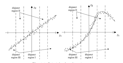
This section discusses how to determine whether the underlying structure within the recorded data is linear or nonlinear. Kruger et al. [38] introduced this nonlinearity test using the principle outlined in Fig. 1.1. The left plot in this figure shows that the first principal component describes the underlying linear relationship between the two variables, $z_{1}$ and $z_{2}$, while the right plot describes some basic nonlinear function, indicated by the curve.
By dividing the operating region into several disjunct regions, where the first region is centered around the origin of the coordinate system, a $\mathrm{PCA}$ model can be obtained from the data of each of these disjunct regions. With respect to Fig. 1.1, this would produce a total of $3 \mathrm{PCA}$ models for each disjunct region in both cases, the linear (left plot) and the nonlinear case (right plot). To determine whether a linear or nonlinear variable interrelationship can be extracted from the data, the principle idea is to take advantage of the residual variance in each of the regions. More precisely, accuracy bounds that are based on the residual variance are obtained for one of the $P C A$ models, for example that of disjunct region I, and the residual variance of the remaining $P C A$ models (for disjunct regions II and III) are benchmarked against these bounds. The test is completed if each of the PCA models has been used to determine accuracy bounds which are then benchmarked against the residual variance of the respective remaining $P C A$ models.
The reason of using the residual variance instead of the variance of the retained score variables is as follows. The residual variance is independent of the region if the underlying interrelationship between the original variables is linear, which the left plot in Fig. $1.1$ indicates. In contrast, observations that have a larger distance from the origin of the coordinate system will, by default, produce a larger projection distance from the origin, that is a larger score value. In this respect, observations that are associated with an
adjunct region that are further outside will logically produce a larger variance irrespective of whether the variable interrelationships are linear or nonlinear.
The detailed presentation of the nonlinearity test in the remainder of this section is structured as follows. Next, the assumptions imposed on the nonlinearity test are shown, prior to a detailed discussion into the construction of disjunct regions. Subsection $3.3$ then shows how to obtain statistical confidence limits for the nondiagonal elements of the correlation matrix. This is followed by the definition of the accuracy bounds. Finally, a summary of the nonlinearity test is presented and some example studies are presented to demonstrate the working of this test.
数据可视化代写
统计代写|数据科学代写data science代考|Principal Component Analysis
PCA 是一种数据分析技术,它依赖于记录观察的简单转换,存储在向量中和∈Rñ, 以产生统计上独立的分数变量,存储在吨∈Rn,n≤ñ :
吨=磷吨和
这里,磷是一个变换矩阵,由正交列向量构成。自首次应用以来磷C一种[21], 该技术已进入广泛的不同应用领域,例如信号处理[75], 因子分析[29,44], 系统识别[77], 化学计量学[20,66]最近,一般数据挖掘[11,58,70]包括图像处理[17,72]和模式识别[10,47],以及过程监控和质量控制[1,82]包括多路[48]、多块[52]和
多尺度 [3] 扩展。这一成功主要与 PCA 能够通过前几个得分变量来描述记录数据中的重要信息/变化的能力有关,这相应地简化了数据分析任务。
西尔维斯特[67]制定了 PCA 背后的想法,在他的工作中消除双线性量词中的冗余,这是多项式表达式,其中指数之和的阶数大于 2,Pearson [51] 通过定义线和多变量空间中与给定点集最接近的平面。Hotelling [28] 然后将这个公式改进为今天使用的公式。在数值上,PCA 与数据协方差或相关矩阵的特征向量-特征值分解密切相关,获得这种分解的数值算法包括迭代 NIPALS 算法 [78],Fisher 和 MacKenzie 早先在[80],以及奇异值分解。关于的很好的概述磷C一种在 Mardia 等人中给出。[45],乔利夫 [32]。沃尔德等人。[80]和杰克逊 [30]。
‘本文的目的是回顾和检查过去二十年来提出的 PCA 的非线性扩展。这是一个重要的研究领域,因为线性 PCA 对非线性数据的应用可能不够充分 [49]。提出非线性 PCA 扩展的第一次尝试包括利用非度量标度进行泛化,这会产生非线性优化问题 [42],并通过给定的点云构建曲线,称为主曲线 [25]。受原始变量重建的启发,和^是(谁)给的:
和^=磷吨=磷(磷吨和)⏟映射 ⏞去映射 ,
这包括分数变量的确定(映射阶段)和和^(去映射阶段),Kramer [37] 提出了一种自关联神经网络(ANN)结构,它通过神经网络层定义映射和去映射阶段。然而,Tan 和 Mavrovouniotis [68] 指出,自关联神经网络的 5 层网络拓扑可能难以训练,即网络权重很难确定层数是否增加 [27]。
为了降低网络复杂度,Tan 和 Mavrovouniotis 提出了一种输入训练 (IT) 网络拓扑,该拓扑省略了映射层。因此,只剩下一个 3 层网络,其中减少的非线性主成分集是作为建立 IT 网络的训练过程的一部分而获得的。Dong 和 McAvoy [16] 引入了一种替代方法,将 5 层自关联网络拓扑划分为两个 3 层拓扑,它们依次表示非线性映射和解映射函数。第一个网络的输出,即映射层,是使用主曲线方法确定的分数变量。
统计代写|数据科学代写data science代考|PCA Preliminaries
在哪里ñ和ķ分别是记录变量的数量和可用观察的数量。定义行和列从通过向量和一世∈Rñ和Gj∈Rķ, 分别,从可以改写如下:
从=[和1吨 和2吨 和3吨 ⋮ 和一世吨 ⋮ 和ķ−1吨 和ķ吨]=[G1 G2G3⋯Gj⋯Gñ]原始集变量的一阶和二阶统计量和吨= (和1和2和3⋯和j⋯和ñ)是:
E{\mathbf{z}}=\mathbf{0} \quad E\left{\mathbf{z z}^{T}\right}=\mathbf{S}{Z Z}E{\mathbf{z}}=\mathbf{0} \quad E\left{\mathbf{z z}^{T}\right}=\mathbf{S}{Z Z}与相关矩阵和被定义为R从从.
PCA 分析需要确定一组分数变量吨ķ,ķ∈123⋯n,n≤ñ,通过应用线性变换和 :
吨ķ=∑j=1ñpķj和j
在参数向量的以下约束下
pķ吨=(pķ1pķ2pķ3⋯pķj⋯pķ ∑j=1ñpķj2=|pķ|2=1.
将分数变量存储在向量中吨吨=(吨1吨2吨3⋯吨j⋯吨n),吨∈Rn具有以下一阶和二阶统计量:
E{\mathbf{t}}=\mathbf{0} \quad E\left{\mathbf{t t}^{T}\right}=\mathbf{\Lambda},E{\mathbf{t}}=\mathbf{0} \quad E\left{\mathbf{t t}^{T}\right}=\mathbf{\Lambda},
在哪里Λ是对角矩阵。的一个重要属性磷C一种是分数变量的方差表示以下最大值:
\lambda_{k}=\arg \max {\mathbf{p}{k}}\left{E\left{t_{k}^{2}\right}\right}=\arg \max {\mathbf{ p}{k}}\left{E\left{\mathbf{p}{k}^{T} \mathbf{z z}^{T} \mathbf{p}{k}\right}\right}\lambda_{k}=\arg \max {\mathbf{p}{k}}\left{E\left{t_{k}^{2}\right}\right}=\arg \max {\mathbf{ p}{k}}\left{E\left{\mathbf{p}{k}^{T} \mathbf{z z}^{T} \mathbf{p}{k}\right}\right}
这是通过以下方式约束:
E\left{\left(\begin{array}{c} t_{1} \ t_{2} \ t_{3} \ \vdots \ t_{k-1} \end{array}\right) t_{k }\right}=0 \quad\left|\mathbf{p}{k}\right|{2}^{2}-1=0E\left{\left(\begin{array}{c} t_{1} \ t_{2} \ t_{3} \ \vdots \ t_{k-1} \end{array}\right) t_{k }\right}=0 \quad\left|\mathbf{p}{k}\right|{2}^{2}-1=0
Anderson [2] 指出,上述约束优化的公式也可以写成:
\lambda_{k}=\arg \max {\mathbf{p}}\left{E\left{\mathbf{p}^{T} \mathbf{z z}^{T} \mathbf{p}\right} -\lambda{k}\left(\mathbf{p}^{T} \mathbf{p}-1\right)\right}\lambda_{k}=\arg \max {\mathbf{p}}\left{E\left{\mathbf{p}^{T} \mathbf{z z}^{T} \mathbf{p}\right} -\lambda{k}\left(\mathbf{p}^{T} \mathbf{p}-1\right)\right}
在假设λķ是预定的。重新制定 (1.11) 以确定pķ导致:\mathbf{p}{k}=\arg \frac{\partial}{\partial \mathbf{p}}\left{E\left{\mathbf{p}^{I} \mathbf{z z ^ { I } } \mathbf{p}\right}-\lambda_{k}\left(\mathbf{p}^{T} \mathbf{p}-1\right)\right}=\mathbf{0}\mathbf{p}{k}=\arg \frac{\partial}{\partial \mathbf{p}}\left{E\left{\mathbf{p}^{I} \mathbf{z z ^ { I } } \mathbf{p}\right}-\lambda_{k}\left(\mathbf{p}^{T} \mathbf{p}-1\right)\right}=\mathbf{0}
并生产
\mathbf{p}{k}=\arg \left{E\left{\mathbf{z z}^{T}\right} \mathbf{p}-2 \lambda{k} \mathbf{p}\right} =\mathbf{0}\mathbf{p}{k}=\arg \left{E\left{\mathbf{z z}^{T}\right} \mathbf{p}-2 \lambda{k} \mathbf{p}\right} =\mathbf{0}
统计代写|数据科学代写data science代考|Nonlinearity Test for PCA Models
本节讨论如何确定记录数据中的底层结构是线性的还是非线性的。克鲁格等人。[38] 使用图 1.1 中概述的原理介绍了这种非线性测试。该图中的左图显示第一个主成分描述了两个变量之间的潜在线性关系,和1和和2,而右图描述了一些基本的非线性函数,由曲线表示。
通过将操作区域划分为几个不相交的区域,其中第一个区域以坐标系的原点为中心,a磷C一种模型可以从这些分离区域中的每一个的数据中获得。对于图 1.1,这将产生总共3磷C一种两种情况下每个分离区域的模型,线性(左图)和非线性情况(右图)。为了确定是否可以从数据中提取线性或非线性变量相互关系,其主要思想是利用每个区域中的残差方差。更准确地说,基于残差方差的准确度界限是针对其中一个获得的磷C一种模型,例如分离区域 I 的模型,以及剩余区域的残差方差磷C一种模型(用于分离区域 II 和 III)以这些界限为基准。如果每个 PCA 模型都已用于确定准确度范围,则测试完成,然后针对相应剩余的剩余方差进行基准测试磷C一种楷模。
使用残差方差而不是保留分数变量的方差的原因如下。如果原始变量之间的潜在相互关系是线性的,则残差方差与区域无关,如图 1 中左图所示。1.1表示。相反,默认情况下,距坐标系原点距离较大的观测值会从原点产生较大的投影距离,即较大的分数值。在这方面,与
无论变量相互关系是线性的还是非线性的,更远的附加区域在逻辑上都会产生更大的方差。
本节其余部分对非线性测试的详细介绍结构如下。接下来,在详细讨论分离区域的构造之前,显示了对非线性测试施加的假设。小节3.3然后显示如何获得相关矩阵的非对角元素的统计置信限。接下来是准确度界限的定义。最后,介绍了非线性测试的摘要,并提供了一些示例研究来证明该测试的工作。

统计代写请认准statistics-lab™. statistics-lab™为您的留学生涯保驾护航。统计代写|python代写代考
随机过程代考
在概率论概念中,随机过程是随机变量的集合。 若一随机系统的样本点是随机函数,则称此函数为样本函数,这一随机系统全部样本函数的集合是一个随机过程。 实际应用中,样本函数的一般定义在时间域或者空间域。 随机过程的实例如股票和汇率的波动、语音信号、视频信号、体温的变化,随机运动如布朗运动、随机徘徊等等。
贝叶斯方法代考
贝叶斯统计概念及数据分析表示使用概率陈述回答有关未知参数的研究问题以及统计范式。后验分布包括关于参数的先验分布,和基于观测数据提供关于参数的信息似然模型。根据选择的先验分布和似然模型,后验分布可以解析或近似,例如,马尔科夫链蒙特卡罗 (MCMC) 方法之一。贝叶斯统计概念及数据分析使用后验分布来形成模型参数的各种摘要,包括点估计,如后验平均值、中位数、百分位数和称为可信区间的区间估计。此外,所有关于模型参数的统计检验都可以表示为基于估计后验分布的概率报表。
广义线性模型代考
广义线性模型(GLM)归属统计学领域,是一种应用灵活的线性回归模型。该模型允许因变量的偏差分布有除了正态分布之外的其它分布。
statistics-lab作为专业的留学生服务机构,多年来已为美国、英国、加拿大、澳洲等留学热门地的学生提供专业的学术服务,包括但不限于Essay代写,Assignment代写,Dissertation代写,Report代写,小组作业代写,Proposal代写,Paper代写,Presentation代写,计算机作业代写,论文修改和润色,网课代做,exam代考等等。写作范围涵盖高中,本科,研究生等海外留学全阶段,辐射金融,经济学,会计学,审计学,管理学等全球99%专业科目。写作团队既有专业英语母语作者,也有海外名校硕博留学生,每位写作老师都拥有过硬的语言能力,专业的学科背景和学术写作经验。我们承诺100%原创,100%专业,100%准时,100%满意。
机器学习代写
随着AI的大潮到来,Machine Learning逐渐成为一个新的学习热点。同时与传统CS相比,Machine Learning在其他领域也有着广泛的应用,因此这门学科成为不仅折磨CS专业同学的“小恶魔”,也是折磨生物、化学、统计等其他学科留学生的“大魔王”。学习Machine learning的一大绊脚石在于使用语言众多,跨学科范围广,所以学习起来尤其困难。但是不管你在学习Machine Learning时遇到任何难题,StudyGate专业导师团队都能为你轻松解决。
多元统计分析代考
基础数据: $N$ 个样本, $P$ 个变量数的单样本,组成的横列的数据表
变量定性: 分类和顺序;变量定量:数值
数学公式的角度分为: 因变量与自变量
时间序列分析代写
随机过程,是依赖于参数的一组随机变量的全体,参数通常是时间。 随机变量是随机现象的数量表现,其时间序列是一组按照时间发生先后顺序进行排列的数据点序列。通常一组时间序列的时间间隔为一恒定值(如1秒,5分钟,12小时,7天,1年),因此时间序列可以作为离散时间数据进行分析处理。研究时间序列数据的意义在于现实中,往往需要研究某个事物其随时间发展变化的规律。这就需要通过研究该事物过去发展的历史记录,以得到其自身发展的规律。
回归分析代写
多元回归分析渐进(Multiple Regression Analysis Asymptotics)属于计量经济学领域,主要是一种数学上的统计分析方法,可以分析复杂情况下各影响因素的数学关系,在自然科学、社会和经济学等多个领域内应用广泛。
MATLAB代写
MATLAB 是一种用于技术计算的高性能语言。它将计算、可视化和编程集成在一个易于使用的环境中,其中问题和解决方案以熟悉的数学符号表示。典型用途包括:数学和计算算法开发建模、仿真和原型制作数据分析、探索和可视化科学和工程图形应用程序开发,包括图形用户界面构建MATLAB 是一个交互式系统,其基本数据元素是一个不需要维度的数组。这使您可以解决许多技术计算问题,尤其是那些具有矩阵和向量公式的问题,而只需用 C 或 Fortran 等标量非交互式语言编写程序所需的时间的一小部分。MATLAB 名称代表矩阵实验室。MATLAB 最初的编写目的是提供对由 LINPACK 和 EISPACK 项目开发的矩阵软件的轻松访问,这两个项目共同代表了矩阵计算软件的最新技术。MATLAB 经过多年的发展,得到了许多用户的投入。在大学环境中,它是数学、工程和科学入门和高级课程的标准教学工具。在工业领域,MATLAB 是高效研究、开发和分析的首选工具。MATLAB 具有一系列称为工具箱的特定于应用程序的解决方案。对于大多数 MATLAB 用户来说非常重要,工具箱允许您学习和应用专业技术。工具箱是 MATLAB 函数(M 文件)的综合集合,可扩展 MATLAB 环境以解决特定类别的问题。可用工具箱的领域包括信号处理、控制系统、神经网络、模糊逻辑、小波、仿真等。