如果你也在 怎样代写数据科学data science这个学科遇到相关的难题,请随时右上角联系我们的24/7代写客服。
数据科学是一个跨学科领域,它使用科学方法、流程、算法和系统从嘈杂的、结构化和非结构化的数据中提取知识和见解,并在广泛的应用领域应用数据的知识和可操作的见解。
statistics-lab™ 为您的留学生涯保驾护航 在代写数据科学data science方面已经树立了自己的口碑, 保证靠谱, 高质且原创的统计Statistics代写服务。我们的专家在代写数据科学data science方面经验极为丰富,各种代写数据科学data science相关的作业也就用不着说。
我们提供的数据科学data science及其相关学科的代写,服务范围广, 其中包括但不限于:
- Statistical Inference 统计推断
- Statistical Computing 统计计算
- Advanced Probability Theory 高等楖率论
- Advanced Mathematical Statistics 高等数理统计学
- (Generalized) Linear Models 广义线性模型
- Statistical Machine Learning 统计机器学习
- Longitudinal Data Analysis 纵向数据分析
- Foundations of Data Science 数据科学基础
统计代写|数据科学代写data science代考|Standard Nonlinear PCA
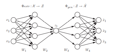
Nonlinear PCA (NLPCA) is based on a multi-layer perceptron (MLP) with an autoassociative topology, also known as an autoencoder, replicator network, bottleneck or sandglass type network. An introduction to multi-layer perceptrons can be found in [28].
The autoassociative network performs an identity mapping. The output $\hat{\boldsymbol{x}}$ is enforced to equal the input $\boldsymbol{x}$ with high accuracy. It is achieved by minimising the squared reconstruction error $E=\frac{1}{2}|\hat{\boldsymbol{x}}-\boldsymbol{x}|^{2}$.
This is a nontrivial task, as there is a ‘bottleneck’ in the middle: a layer of fewer units than at the input or output layer. Thus, the data have to be projected or compressed into a lower dimensional representation $Z$.
The network can be considered to consist of two parts: the first part represents the extraction function $\Phi_{\text {extr }}: \mathcal{X} \rightarrow \mathcal{Z}$, whereas the second part represents the inverse function, the generation or reconstruction function $\Phi_{g e n}: \mathcal{Z} \rightarrow \hat{\mathcal{X}}$. A hidden layer in each part enables the network to perform nonlinear mapping functions. Without these hidden layers, the network would only be able to perform linear PCA even with nonlinear units in the component layer, as shown by Bourlard and Kamp [29]. To regularise the network, a weight decay term is added $E_{\text {total }}=E+\nu \sum_{i} w_{i}^{2}$ in order to penalise large network weights $w$. In most experiments, $\nu=0.001$ was a reasonable choice.
In the following, we describe the applied network topology by the notation $l_{1}-l_{2}-l_{3} \ldots-l_{S}$ where $l_{s}$ is the number of units in layer $s$. For example, 3-4-1-4-3 specifies a network of five layers having three units in the input and output layer, four units in both hidden layers, and one unit in the component layer, as illustrated in Flg. $2.2$.
统计代写|数据科学代写data science代考|Hierarchical nonlinear PCA
In order to decompose data in a PCA related way, linearly or nonlinearly, it is important to distinguish applications of pure dimensionality reduction from applications where the identification and discrimination of unique and meaningful components is of primary interest, usually referred to as feature extraction. In applications of pure dimensionality reduction with clear emphasis on noise reduction and data compression, only a subspace with high descriptive capacity is requred. How the individual components form this subspace is not particularly constrained and hence does not need to be unique. The only requirement is that the subspace explains maximal information in the mean squared error sense. Since the individual components which span this subspace, are treated equally by the algorithm without any particular order or differential weighting, this is referred to as symmetric type of learning. This includes the nonlinear PCA performed by the standard autoassociative neural network which is therefore referred to as s-NLPCA.
By contrast, hierarchical nonlinear PCA $(h-N L P C A)$, as proposed by Scholz and Vigário [10], provides not only the optimal nonlinear subspace spanned by components, it also constrains the nonlinear components to have the same hierarchical order as the linear components in standard PCA.
Hierarchy, in this context, is explained by two important properties: scalability and stability. Scalability means that the first $n$ components explain the maximal variance that can be covered by a $n$-dimensional subspace. Stability means that the i-th component of an $n$ component solution is identical to the $i$-th component of an $m$ component solution.
统计代写|数据科学代写data science代考|The Hierarchical Error Function
$E_{1}$ and $E_{1,2}$ are the squared reconstruction errors when using only the first or both the first and the second component, respectively. In order to perform the h-NLPCA, we have to impose not only a small $E_{1,2}$ (as in s-NLPCA), but also a small $E_{1}$. This can be done by minimising the hierarchical error:
$$
E_{H}=E_{1}+E_{1,2}
$$
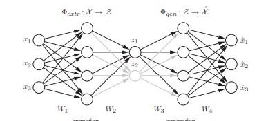
Fig. 2.3. Hierarchical NLPCA. The standard autoassociative network is hierarchically extended to perform the hierarchical NLPCA (h-NLPCA). In addition to the whole 3-4-2-4-3 network (grey+black), there is a 3-4-1-4-3 subnetwork (black) explicitly considered. The component layer in the middle has either one or two units which represent the tirst and second components, respectively. Both the error $E_{1}$ of the subnotwork with one componont and the srror of the total network with two components are estimated in each iteration. The network weights are then adapted at once with regard to the total hierarchic error $E=E_{1}+E_{1,2}$
To find the optimal network weights for a minimal error in the h-NLPCA as well as in the standard symmetric approach, the conjugate gradient descent algorithm [31] is used. At each iteration, the single error terms $E_{1}$ and $E_{1,2}$ have to be calculated separately. This is performed in the standard s-NLP $\overline{\mathrm{C} A}$ way by a network either with one or with two units in the component layer. Here, one network is the subnetwork of the other, as illustrated in Fig. 2.3. The gradient $\nabla E_{H}$ is the sum of the individual gradients $\nabla E_{H}=\nabla E_{1}+\nabla E_{1,2}$. If a weight $w_{i}$ does not exist in the subnetwork, $\frac{\partial E_{1}}{\partial w_{i}}$ is set to zero.
To achieve more robust results, the network weights are set such that the sigmoidal nonlinearities work in the linear range, corresponding to initialise the network with the simple linear PCA solution.
The hierarchical error function (2.1) can be easily extended to $k$ components $(k \leq d)$ :
$$
E_{H}=E_{1}+E_{1,2}+E_{1,2,3}+\cdots+E_{1,2,3, \ldots, k} .
$$
The hierarchical condition as given by $E_{H}$ can then be interpreted as follows: we search for a $k$-dimensional subspace of minimal mean square error (MSE) under the constraint that the $(k-1)$-dimensional subspace is also of minimal MSE. This is successively extended such that all $1, \ldots, k$ dimensional subspaces are of minimal MSE. Hence, each subspace represents the data with regard to its dimensionalities best. Hierarchical nonlinear PCA can therefore be seen as a true and natural nonlinear extension of standard linear PCA.
数据可视化代写
统计代写|数据科学代写data science代考|Standard Nonlinear PCA
非线性 PCA (NLPCA) 基于具有自关联拓扑的多层感知器 (MLP),也称为自动编码器、复制器网络、瓶颈或沙漏型网络。多层感知器的介绍可以在[28]中找到。
自关联网络执行身份映射。输出X^强制等于输入X具有高精度。它是通过最小化平方重建误差来实现的和=12|X^−X|2.
这是一项不平凡的任务,因为中间有一个“瓶颈”:一个单元比输入或输出层少的层。因此,必须将数据投影或压缩为较低维度的表示从.
网络可以认为由两部分组成:第一部分表示提取函数披提取物 :X→从,而第二部分表示反函数,即生成或重建函数披G和n:从→X^. 每个部分中的隐藏层使网络能够执行非线性映射功能。如果没有这些隐藏层,即使在组件层中有非线性单元,网络也只能执行线性 PCA,如 Bourlard 和 Kamp [29] 所示。为了规范网络,添加了权重衰减项和全部的 =和+ν∑一世在一世2为了惩罚大的网络权重在. 在大多数实验中,ν=0.001是一个合理的选择。
下面,我们用符号描述应用的网络拓扑l1−l2−l3…−l小号在哪里ls是层中的单元数s. 例如,3-4-1-4-3 指定了一个五层的网络,在输入和输出层中具有三个单元,在两个隐藏层中具有四个单元,在组件层中具有一个单元,如图所示。2.2.
统计代写|数据科学代写data science代考|Hierarchical nonlinear PCA
为了以与 PCA 相关的方式(线性或非线性)分解数据,将纯降维的应用与主要关注唯一和有意义的组件的识别和区分(通常称为特征提取)的应用区分开来是很重要的。在明确强调降噪和数据压缩的纯降维应用中,只需要具有高描述能力的子空间。单个组件如何形成这个子空间并没有特别的限制,因此不需要是唯一的。唯一的要求是子空间在均方误差意义上解释最大信息。由于跨越该子空间的各个组件被算法平等对待,没有任何特定的顺序或差异加权,这被称为对称类型的学习。这包括由标准自联想神经网络执行的非线性 PCA,因此称为 s-NLPCA。
相比之下,分层非线性 PCA(H−ñ大号磷C一种),正如 Scholz 和 Vigário [10] 所提出的,它不仅提供了由分量跨越的最优非线性子空间,而且还约束非线性分量与标准 PCA 中的线性分量具有相同的层次顺序。
在这种情况下,层次结构由两个重要属性来解释:可扩展性和稳定性。可扩展性意味着第一个n组件解释了一个可以覆盖的最大方差n维子空间。稳定性意味着第 i 个分量n组件解决方案是相同的一世-第一个组件米组件解决方案。
统计代写|数据科学代写data science代考|The Hierarchical Error Function
和1和和1,2分别是仅使用第一个或同时使用第一个和第二个分量时的平方重建误差。为了执行 h-NLPCA,我们不仅要强加一个小的和1,2(如在 s-NLPCA 中),但也是一个小的和1. 这可以通过最小化层次误差来完成:
和H=和1+和1,2
图 2.3。分层 NLPCA。标准的自关联网络被分层扩展以执行分层 NLPCA (h-NLPCA)。除了整个 3-4-2-4-3 网络(灰色+黑色)之外,还明确考虑了一个 3-4-1-4-3 子网络(黑色)。中间的组件层有一个或两个单元,分别代表第一个和第二个组件。两者的错误和1在每次迭代中估计具有一个组件的子网络和具有两个组件的整个网络的 srror。然后根据总的层次误差立即调整网络权重和=和1+和1,2
为了在 h-NLPCA 和标准对称方法中找到最小误差的最佳网络权重,使用了共轭梯度下降算法 [31]。在每次迭代中,单个误差项和1和和1,2必须单独计算。这是在标准 s-NLP 中执行的C一种¯通过在组件层中具有一个或两个单元的网络。这里,一个网络是另一个网络的子网络,如图 2.3 所示。梯度∇和H是各个梯度的总和∇和H=∇和1+∇和1,2. 如果一个重量在一世子网中不存在,∂和1∂在一世设置为零。
为了获得更稳健的结果,网络权重被设置为使 sigmoidal 非线性工作在线性范围内,对应于用简单的线性 PCA 解决方案初始化网络。
层次误差函数(2.1)可以很容易地扩展到ķ组件(ķ≤d) :
和H=和1+和1,2+和1,2,3+⋯+和1,2,3,…,ķ.
给定的分层条件和H然后可以解释如下:我们搜索一个ķ- 最小均方误差 (MSE) 的维子空间,约束条件为(ķ−1)维子空间也是最小 MSE。这被连续扩展,使得所有1,…,ķ维子空间具有最小 MSE。因此,每个子空间就其维度而言最好地表示数据。因此,分层非线性 PCA 可以被视为标准线性 PCA 的真实和自然的非线性扩展。

统计代写请认准statistics-lab™. statistics-lab™为您的留学生涯保驾护航。统计代写|python代写代考
随机过程代考
在概率论概念中,随机过程是随机变量的集合。 若一随机系统的样本点是随机函数,则称此函数为样本函数,这一随机系统全部样本函数的集合是一个随机过程。 实际应用中,样本函数的一般定义在时间域或者空间域。 随机过程的实例如股票和汇率的波动、语音信号、视频信号、体温的变化,随机运动如布朗运动、随机徘徊等等。
贝叶斯方法代考
贝叶斯统计概念及数据分析表示使用概率陈述回答有关未知参数的研究问题以及统计范式。后验分布包括关于参数的先验分布,和基于观测数据提供关于参数的信息似然模型。根据选择的先验分布和似然模型,后验分布可以解析或近似,例如,马尔科夫链蒙特卡罗 (MCMC) 方法之一。贝叶斯统计概念及数据分析使用后验分布来形成模型参数的各种摘要,包括点估计,如后验平均值、中位数、百分位数和称为可信区间的区间估计。此外,所有关于模型参数的统计检验都可以表示为基于估计后验分布的概率报表。
广义线性模型代考
广义线性模型(GLM)归属统计学领域,是一种应用灵活的线性回归模型。该模型允许因变量的偏差分布有除了正态分布之外的其它分布。
statistics-lab作为专业的留学生服务机构,多年来已为美国、英国、加拿大、澳洲等留学热门地的学生提供专业的学术服务,包括但不限于Essay代写,Assignment代写,Dissertation代写,Report代写,小组作业代写,Proposal代写,Paper代写,Presentation代写,计算机作业代写,论文修改和润色,网课代做,exam代考等等。写作范围涵盖高中,本科,研究生等海外留学全阶段,辐射金融,经济学,会计学,审计学,管理学等全球99%专业科目。写作团队既有专业英语母语作者,也有海外名校硕博留学生,每位写作老师都拥有过硬的语言能力,专业的学科背景和学术写作经验。我们承诺100%原创,100%专业,100%准时,100%满意。
机器学习代写
随着AI的大潮到来,Machine Learning逐渐成为一个新的学习热点。同时与传统CS相比,Machine Learning在其他领域也有着广泛的应用,因此这门学科成为不仅折磨CS专业同学的“小恶魔”,也是折磨生物、化学、统计等其他学科留学生的“大魔王”。学习Machine learning的一大绊脚石在于使用语言众多,跨学科范围广,所以学习起来尤其困难。但是不管你在学习Machine Learning时遇到任何难题,StudyGate专业导师团队都能为你轻松解决。
多元统计分析代考
基础数据: $N$ 个样本, $P$ 个变量数的单样本,组成的横列的数据表
变量定性: 分类和顺序;变量定量:数值
数学公式的角度分为: 因变量与自变量
时间序列分析代写
随机过程,是依赖于参数的一组随机变量的全体,参数通常是时间。 随机变量是随机现象的数量表现,其时间序列是一组按照时间发生先后顺序进行排列的数据点序列。通常一组时间序列的时间间隔为一恒定值(如1秒,5分钟,12小时,7天,1年),因此时间序列可以作为离散时间数据进行分析处理。研究时间序列数据的意义在于现实中,往往需要研究某个事物其随时间发展变化的规律。这就需要通过研究该事物过去发展的历史记录,以得到其自身发展的规律。
回归分析代写
多元回归分析渐进(Multiple Regression Analysis Asymptotics)属于计量经济学领域,主要是一种数学上的统计分析方法,可以分析复杂情况下各影响因素的数学关系,在自然科学、社会和经济学等多个领域内应用广泛。
MATLAB代写
MATLAB 是一种用于技术计算的高性能语言。它将计算、可视化和编程集成在一个易于使用的环境中,其中问题和解决方案以熟悉的数学符号表示。典型用途包括:数学和计算算法开发建模、仿真和原型制作数据分析、探索和可视化科学和工程图形应用程序开发,包括图形用户界面构建MATLAB 是一个交互式系统,其基本数据元素是一个不需要维度的数组。这使您可以解决许多技术计算问题,尤其是那些具有矩阵和向量公式的问题,而只需用 C 或 Fortran 等标量非交互式语言编写程序所需的时间的一小部分。MATLAB 名称代表矩阵实验室。MATLAB 最初的编写目的是提供对由 LINPACK 和 EISPACK 项目开发的矩阵软件的轻松访问,这两个项目共同代表了矩阵计算软件的最新技术。MATLAB 经过多年的发展,得到了许多用户的投入。在大学环境中,它是数学、工程和科学入门和高级课程的标准教学工具。在工业领域,MATLAB 是高效研究、开发和分析的首选工具。MATLAB 具有一系列称为工具箱的特定于应用程序的解决方案。对于大多数 MATLAB 用户来说非常重要,工具箱允许您学习和应用专业技术。工具箱是 MATLAB 函数(M 文件)的综合集合,可扩展 MATLAB 环境以解决特定类别的问题。可用工具箱的领域包括信号处理、控制系统、神经网络、模糊逻辑、小波、仿真等。