ECE4110 - 统计代写答疑辅导

标签： ECE4110

电气工程代写|数字系统设计作业代写Digital System Design代考|COE328

Posted on 2022年10月22日2022年10月22日 by statistics-lab

如果你也在怎样代写数字系统设计Digital System Design这个学科遇到相关的难题，请随时右上角联系我们的24/7代写客服。

数字系统设计课程侧重于从头开始设计数字系统。该课程的重点是设计组合和顺序构件，使用这些构件来设计更大的数字系统。

statistics-lab™ 为您的留学生涯保驾护航在代写数字系统设计Digital System Design方面已经树立了自己的口碑, 保证靠谱, 高质且原创的统计Statistics代写服务。我们的专家在代写数字系统设计Digital System Design方面经验极为丰富，各种代写数字系统设计Digital System Design相关的作业也就用不着说。

我们提供的数字系统设计Digital System Design及其相关学科的代写，服务范围广, 其中包括但不限于:

Statistical Inference 统计推断
Statistical Computing 统计计算
Advanced Probability Theory 高等楖率论
Advanced Mathematical Statistics 高等数理统计学
(Generalized) Linear Models 广义线性模型
Statistical Machine Learning 统计机器学习
Longitudinal Data Analysis 纵向数据分析
Foundations of Data Science 数据科学基础

电气工程代写|数字系统设计作业代写Digital System Design代考|COE328

电气工程代写|数字系统设计作业代写Digital System Design代考|Transmitter Antenna Losses

Several losses are associated with the antenna. Some of the possible losses, which may or may not be present in each antenna, are as follows:

$L_{t r}$, radome losses on the transmitter antenna. The radome is the covering over the antenna that protects the antenna from the outside elements. Most antennas do not require a radome.
$L_{t p o l}$, polarization mismatch losses. Many antennas are polarized (i.e., horizontal, vertical, or circular). This defines the spatial position or orientation of the electric and magnetic fields. A mismatch loss is due to the polarization of the transmitter antenna being spatially off with respect to the receiver antenna. The amount of loss is equal to the angle difference between them. For example, if both the receiver and transmitter antennas are vertically polarized, they would be at $90^{\circ}$ from the earth. If one is positioned at $80^{\circ}$ and the other is positioned at $100^{\circ}$, the difference is $20^{\circ}$. Therefore, the loss due to polarization would be
$$
20 \log (\cos \theta)=20 \log (\cos 20)=0.54 \mathrm{~dB}
$$
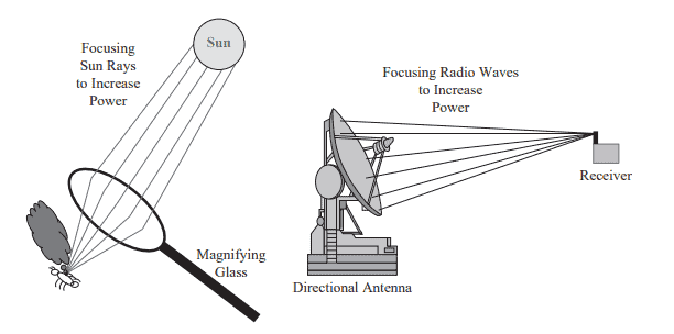
$L_{t f o c}$, focusing loss or refractive loss. This is caused by imperfections in the shape of the antenna so that the energy is focused toward the feed. This is often a factor when the antenna receives signals at low elevation angles.
$L_{\text {tpoint }}$, mispointed loss. This is caused by transmitting and receiving directional antennas that are not exactly lined up and pointed toward each other. Thus, the gains of the antennas do not add up without a loss of signal power.
$L_{\text {tcon, }}$ conscan crossover loss. This loss is present only if the antenna is scanned in a circular search pattern, such as a conscan (conical scan) radar searching for a target. Conscan means that the antenna system is either electrically or mechanically scanned in a conical fashion or in a cone-shaped pattern. This is used in radar and other systems that desire a broader band of spatial coverage but must maintain a narrow beam width. This is also used for generating the pointing error for a tracking antenna.

电气工程代写|数字系统设计作业代写Digital System Design代考|Transmitted Effective Isotropic Radiated Power

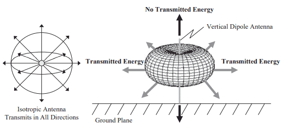
An isotropic radiator is a theoretical radiator that assumes a point source radiating in all directions. Effective isotropic radiated power (EIRP) is the amount of power from a single point radiator that is required to equal the amount of power that is transmitted by the power amplifier, losses, and directivity of the antenna (antenna gain) in the direction of the receiver.

The EIRP provides a way to compare different transmitters. To analyze the output of an antenna, EIRP is used (Figure 1-2):
$$
\operatorname{EIRP}=P_t-L_{t t}+G_t-L_{t o}
$$
where
$P_t=$ transmitter power in $\mathrm{dBm}$
$L_{t t}=$ total negative losses in $\mathrm{dB}$; coaxial or waveguide line losses, switchers, circulators, antenna connections
$G_t=$ transmitter antenna gain in $\mathrm{dB}$ referenced to a isotropic antenna
$L_{t a}=$ total transmitter antenna losses in $\mathrm{dB}$
Effective radiated power (ERP) is another term used to describe the output power of an antenna. However, instead of comparing the effective power to an isotropic radiator, the power output of the antenna is compared to a dipole antenna. The relationship between EIRP and ERP is
$$
\mathrm{EIRP}=\mathrm{ERP}+G_{\text {dipole }},
$$
where $G_{\text {dipole }}$ is the gain of a dipole antenna, which is equal to approximately $2.14 \mathrm{~dB}$ (Figure 1-2). For example,
$$
\begin{aligned}
\mathrm{EIRP} &=10 \mathrm{dBm} \
\mathrm{ERP} &=\mathrm{EIRP}-G_{\text {dipole }}=10 \mathrm{dBm}-2.14 \mathrm{~dB}=7.86 \mathrm{dBm}
\end{aligned}
$$

数字系统设计代考

电气工程代写|数字系统设计作业代写Digital System Design代考|Transmitter Antenna Losses

一些损耗与天线有关。每个天线中可能存在也可能不存在的一些可能的损耗如下:

$L_{t r}$ ，发射机天线上的天线罩损耗。天线罩是天线上的覆盖物，可保护天线免受外部元件的影响。大多数天线不需要天线罩。
$L_{t p o l}$ ，极化失配损失。许多天线是极化的（即水平、垂直或圆形）。这定义了电场和磁场的空间位置或方向。失配损耗是由于发射器天线的极化相对于接收器天线在空间上偏离。损失量等于它们之间的角度差。例如，如果接收器和发射器天线都是垂直极化的，它们将在 $90^{\circ}$ 来自地球。如果一个位于 $80^{\circ}$ 另一个位于 $100^{\circ}$ ，区别是 $20^{\circ}$. 因此，极化引起的损耗为
$$
20 \log (\cos \theta)=20 \log (\cos 20)=0.54 \mathrm{~dB}
$$
$L_{t f o c}$ ，聚焦损失或屈光损失。这是由天线形状的缺陷引起的，因此能量集中在馈源上。当天线以低仰角接收信号时，这通常是一个因素。
$L_{\text {tpoint }}$ ，误点损失。这是由于发射和接收定向天线末完全对齐并相互指向造成的。因此，天线的增益不会在没有信号功率损失的情况下相加。
$L_{\text {tcon, }}$ conscan 交叉损失。仅当以圆形搜索模式扫描天线时才会出现这种损失，例如搜索目标的 conscan (锥形扫描) 雷达。Conscan 意味着天线系统以雉形方式或以雉形图案进行电气或机械扫描。这用于雷达和其他需要更宽的空间覆盖范围但必须保持窄波束宽度的系统。这也用于生成跟踪天线的指向误差。

电气工程代写|数字系统设计作业代写Digital System Design代考|Transmitted Effective Isotropic Radiated Power

各向同性辐射体是一种理论辐射体，它假设点源向所有方向辐射。有效全向辐射功率 (EIRP) 是来自单点辐射器的功率量，它需要等于功率放大器发射的功率量、损耗和天线方向上的天线方向性 (天线增益)。接收者。
EIRP 提供了一种比较不同发射机的方法。为了分析天线的输出，使用了 EIRP (图 1-2)：
$$
\mathrm{EIRP}=P_t-L_{t t}+G_t-L_{t o}
$$
在哪里
$P_t=$ 发射机功率 $\mathrm{dBm}$
$L_{t t}=$ 总负损失 $\mathrm{dB} ;$ 同轴或波导线路损耗、开关、环行器、天线连接
$G_t=$ 发射机天线增益 $\mathrm{dB}$ 参考各向同性天线
$L_{t a}=$ 总发射机天线损耗 $\mathrm{dB}$
有效辐射功率 (ERP) 是用于描述天线输出功率的另一个术语。但是，不是将有效功率与各向同性辐射器进行比较，而是将天线的功率输出与偶极天线进行比较。EIRP和ERP之间的关系是
$$
\mathrm{EIRP}=\mathrm{ERP}+G_{\text {dipole }},
$$
在哪里 $G_{\text {dipole }}$ 是偶极天线的增益，大约等于 $2.14 \mathrm{~dB}$ (图 1-2) 。例如，
$$
\mathrm{EIRP}=10 \mathrm{dBm} \mathrm{ERP} \quad=\mathrm{EIRP}-G_{\text {dipole }}=10 \mathrm{dBm}-2.14 \mathrm{~dB}=7.86 \mathrm{dBm}
$$

电气工程代写|数字系统设计作业代写Digital System Design代考请认准statistics-lab™

统计代写请认准statistics-lab™. statistics-lab™为您的留学生涯保驾护航。统计代写|python代写代考

随机过程代考

在概率论概念中，随机过程是随机变量的集合。若一随机系统的样本点是随机函数，则称此函数为样本函数，这一随机系统全部样本函数的集合是一个随机过程。实际应用中，样本函数的一般定义在时间域或者空间域。 随机过程的实例如股票和汇率的波动、语音信号、视频信号、体温的变化，随机运动如布朗运动、随机徘徊等等。

贝叶斯方法代考

贝叶斯统计概念及数据分析表示使用概率陈述回答有关未知参数的研究问题以及统计范式。后验分布包括关于参数的先验分布，和基于观测数据提供关于参数的信息似然模型。根据选择的先验分布和似然模型，后验分布可以解析或近似，例如，马尔科夫链蒙特卡罗 (MCMC) 方法之一。贝叶斯统计概念及数据分析使用后验分布来形成模型参数的各种摘要，包括点估计，如后验平均值、中位数、百分位数和称为可信区间的区间估计。此外，所有关于模型参数的统计检验都可以表示为基于估计后验分布的概率报表。

广义线性模型代考

广义线性模型（GLM）归属统计学领域，是一种应用灵活的线性回归模型。该模型允许因变量的偏差分布有除了正态分布之外的其它分布。

statistics-lab作为专业的留学生服务机构，多年来已为美国、英国、加拿大、澳洲等留学热门地的学生提供专业的学术服务，包括但不限于Essay代写，Assignment代写，Dissertation代写，Report代写，小组作业代写，Proposal代写，Paper代写，Presentation代写，计算机作业代写，论文修改和润色，网课代做，exam代考等等。写作范围涵盖高中，本科，研究生等海外留学全阶段，辐射金融，经济学，会计学，审计学，管理学等全球99%专业科目。写作团队既有专业英语母语作者，也有海外名校硕博留学生，每位写作老师都拥有过硬的语言能力，专业的学科背景和学术写作经验。我们承诺100%原创，100%专业，100%准时，100%满意。

机器学习代写

随着AI的大潮到来，Machine Learning逐渐成为一个新的学习热点。同时与传统CS相比，Machine Learning在其他领域也有着广泛的应用，因此这门学科成为不仅折磨CS专业同学的“小恶魔”，也是折磨生物、化学、统计等其他学科留学生的“大魔王”。学习Machine learning的一大绊脚石在于使用语言众多，跨学科范围广，所以学习起来尤其困难。但是不管你在学习Machine Learning时遇到任何难题，StudyGate专业导师团队都能为你轻松解决。

多元统计分析代考

基础数据: $N$ 个样本， $P$ 个变量数的单样本，组成的横列的数据表
变量定性: 分类和顺序；变量定量：数值
数学公式的角度分为: 因变量与自变量

时间序列分析代写

随机过程，是依赖于参数的一组随机变量的全体，参数通常是时间。随机变量是随机现象的数量表现，其时间序列是一组按照时间发生先后顺序进行排列的数据点序列。通常一组时间序列的时间间隔为一恒定值（如1秒，5分钟，12小时，7天，1年），因此时间序列可以作为离散时间数据进行分析处理。研究时间序列数据的意义在于现实中，往往需要研究某个事物其随时间发展变化的规律。这就需要通过研究该事物过去发展的历史记录，以得到其自身发展的规律。

回归分析代写

多元回归分析渐进（Multiple Regression Analysis Asymptotics）属于计量经济学领域，主要是一种数学上的统计分析方法，可以分析复杂情况下各影响因素的数学关系，在自然科学、社会和经济学等多个领域内应用广泛。

MATLAB代写

MATLAB 是一种用于技术计算的高性能语言。它将计算、可视化和编程集成在一个易于使用的环境中，其中问题和解决方案以熟悉的数学符号表示。典型用途包括：数学和计算算法开发建模、仿真和原型制作数据分析、探索和可视化科学和工程图形应用程序开发，包括图形用户界面构建MATLAB 是一个交互式系统，其基本数据元素是一个不需要维度的数组。这使您可以解决许多技术计算问题，尤其是那些具有矩阵和向量公式的问题，而只需用 C 或 Fortran 等标量非交互式语言编写程序所需的时间的一小部分。MATLAB 名称代表矩阵实验室。MATLAB 最初的编写目的是提供对由 LINPACK 和 EISPACK 项目开发的矩阵软件的轻松访问，这两个项目共同代表了矩阵计算软件的最新技术。MATLAB 经过多年的发展，得到了许多用户的投入。在大学环境中，它是数学、工程和科学入门和高级课程的标准教学工具。在工业领域，MATLAB 是高效研究、开发和分析的首选工具。MATLAB 具有一系列称为工具箱的特定于应用程序的解决方案。对于大多数 MATLAB 用户来说非常重要，工具箱允许您学习和应用专业技术。工具箱是 MATLAB 函数（M 文件）的综合集合，可扩展 MATLAB 环境以解决特定类别的问题。可用工具箱的领域包括信号处理、控制系统、神经网络、模糊逻辑、小波、仿真等。

R语言代写	问卷设计与分析代写
PYTHON代写	回归分析与线性模型代写
MATLAB代写	方差分析与试验设计代写
STATA代写	机器学习/统计学习代写
SPSS代写	计量经济学代写
EVIEWS代写	时间序列分析代写
EXCEL代写	深度学习代写
SQL代写	各种数据建模与可视化代写

电气工程代写|数字系统设计作业代写Digital System Design代考|EE301

Posted on 2022年10月22日2022年10月22日 by statistics-lab

如果你也在怎样代写数字系统设计Digital System Design这个学科遇到相关的难题，请随时右上角联系我们的24/7代写客服。

数字系统设计课程侧重于从头开始设计数字系统。该课程的重点是设计组合和顺序构件，使用这些构件来设计更大的数字系统。

我们提供的数字系统设计Digital System Design及其相关学科的代写，服务范围广, 其中包括但不限于:

Statistical Inference 统计推断
Statistical Computing 统计计算
Advanced Probability Theory 高等楖率论
Advanced Mathematical Statistics 高等数理统计学
(Generalized) Linear Models 广义线性模型
Statistical Machine Learning 统计机器学习
Longitudinal Data Analysis 纵向数据分析
Foundations of Data Science 数据科学基础

电气工程代写|数字系统设计作业代写Digital System Design代考|EE301

电气工程代写|数字系统设计作业代写Digital System Design代考|Transmitter Component Losses

Most transceiver systems contain RF components such as a circulator or a transmit/receive (T/R) switch that enable the transceiver to use the same antenna for both transmitting and receiving. Also, if the antenna arrays use multiple antennas, some of their components will interconnect the individual antenna elements. Since these elements have a loss associated with them, they need to be taken into account in the overall output power of the transmitter. These losses directly reduce the signal level or the power output of the transmitter. The component losses are labeled and are included in the analysis:
$L_{\text {tcomp }}=$ switchers, circulators, antenna connections
Whichever method is used, the losses directly affect the power output on a one-for-one basis. A $1 \mathrm{~dB}$ loss equals a $1 \mathrm{~dB}$ loss in transmitted power. Therefore, the losses after the final output power amplifier (PA) of the transmitter and the first amplifier (or low-noise amplifier [LNA]) of the receiver should be kept to a minimum. Each $\mathrm{dB}$ of loss in this path will either reduce the minimum detectable signal (MDS) by a dB or the transmitter gain will have to transmit a $\mathrm{dB}$ more power.

Since most transmitters are located at a distance from the antenna, the cable or waveguide connecting the transmitter to the antenna contains losses that need to be incorporated in the total power output:
$L_{t l l}=$ coaxial or waveguide line losses (in $\left.\mathrm{dB}\right)$
These transmitter line losses are included in the total power output analysis; a $1 \mathrm{~dB}$ loss equals a $1 \mathrm{~dB}$ loss in power output. Using larger diameter cables or higher quality cables can reduce the loss, which is a trade-off with cost. For example, heliax cables are used for very low-loss applications. However, they are generally more expensive and larger in diameter than standard cables. The total losses between the power amplifier and the antenna are therefore equal to
$$
L_{t t}=L_{t l l}+L_{\text {tcomp }}
$$
Another way to reduce the loss between the transmitter and the antenna is to locate the transmitter power amplifier as close to the antenna as possible. This will reduce the length of the cable, which reduces the overall loss in the transmitter.

电气工程代写|数字系统设计作业代写Digital System Design代考|Transmitter Antenna Gain

Most antennas experience gain because they tend to focus energy in specified directions compared with an ideal isotropic antenna, which radiates in all directions. Antennas do not amplify the signal power but focus the existing signal in a given direction. This is similar to a magnifying glass, which can be used to focus the sun rays in a specific direction, increasing the signal level at a single point (Figure 1-4).

A simple vertical dipole antenna experiences approximately $2.14 \mathrm{dBi}$ of gain compared with an isotropic radiator because it transmits most of the signal around the antenna, with very little of the signal transmitted directly up to the sky and directly down to the ground (Figure 1-5).
A parabolic dish radiator is commonly used at high frequencies to achieve gain by focusing the signal in the direction the antenna is pointing (Figure 1-6). The gain for a parabolic antenna is
$$
G_t=10 \log \left[n(\pi D / \lambda)^2\right]
$$
where
$$
\begin{aligned}
G_t &=\text { gain of the antenna (in dBi) } \
n &=\text { efficiency factor }<1 \
D &=\text { diameter of the parabolic dish } \
\lambda &=\text { wavelength }
\end{aligned}
$$

The efficiency factor is the actual gain of the antenna compared with the theoretical gain. This can happen when a parabolic antenna is not quite parabolic, when the surface of the antenna combined with the feed is not uniform, and when other anomalies occur in the actual implementation of the antenna system. Typically this ranges from $0.5$ to $0.8$, depending on the design and the frequency of operation.

Notice that the antenna gain increases both with increasing diameter and higher frequency (shorter wavelength). The gain of the antenna is a direct gain where a $1 \mathrm{~dB}$ gain equals a $1 \mathrm{~dB}$ improvement in the transmitter power output. Therefore, a larger gain will increase the range of the link. In addition, the more gain the antenna can produce, the less power the power amplifier has to deliver for the same range. This is another trade-off that needs to be considered to ensure the best design and the lowest cost for a given application.

数字系统设计代考

电气工程代写|数字系统设计作业代写Digital System Design代考|Transmitter Component Losses

大多数收发器系统都包含射频组件，例如循环器或发射/接收 (T/R) 开关，使收发器能够使用相同的天线进行发射和接收。此外，如果天线阵列使用多个天线，它们的一些组件将互连各个天线元件。由于这些元件具有与之相关的损耗，因此需要在发射器的总输出功率中考虑它们。这些损耗直接降低了发射机的信号电平或功率输出。组件损耗已标记并包含在分析中:
$L_{\text {tcomp }}=$ 切换器、循环器、天线连接
无论使用哪种方法，损耗都会一对一地直接影响功率输出。一个 $1 \mathrm{~dB}$ 损失等于 $1 \mathrm{~dB}$ 传输功率的损失。因此，发射器的最终输出功率放大器 (PA) 和接收器的第一个放大器 (或低䆆声放大器 $[L N A])$ 后的损耗应保持在最低水平。每个dB这条路径中的损耗要么将最小可检测信号 (MDS) 降低一个 $\mathrm{dB}$ ，要么发射器增益将不得不发射一个 $\mathrm{dB}$ 更多的权力。
由于大多数发射器与天线相距一定距离，因此将发射器连接到天线的电赀或波导包含需要纳入总功率输出的损耗: $L_{t l l}=$ 同轴或波导线损耗 (在 $\left.\mathrm{dB}\right)$
这些发射机线路损耗包含在总功率输出分析中; 一个 $1 \mathrm{~dB}$ 损失等于 $1 \mathrm{~dB}$ 功率输出的损失。使用更大直径的电笕或更高质量的电缆可以减少损耗，这是与成本的权衡。例如，螺旋电缆用于非常低损耗的应用。但是，它们通常比标准电跕更昂贵且直径更大。因此，功率放大器和天线之间的总损耗等于
$$
L_{t t}=L_{t l l}+L_{\text {tcomp }}
$$
另一种减少发射机和天线之间损耗的方法是将发射机功率放大器放置在尽可能靠近天线的位置。这将减少电趿的长度，从而降低发射机的整体损耗。

电气工程代写|数字系统设计作业代写Digital System Design代考|Transmitter Antenna Gain

大多数天线都能获得增益，因为与理想的各向同性天线相比，它们倾向于将能量集中在特定的方向上，而理想的各向同性天线佘向所有方向辐射。天线不会放大信号功率，而是将现有信号集中在给定方向上。这类似于放大镜，可用于将太阳光线聚焦到特定方向，从而增加单个点的信号电平 (图 1-4)。
一个简单的垂直偶极子天线大约经历 $2.14 \mathrm{dBi}$ 与各向同性辐射器相比，它的增益比各向同性辐射器高，因为它在天线周围传输大部分信号，只有很少的信号直接向上传输到天空并直接向下传输到地面（图 1-5)。
抛物面碟形辐射器通常用于高频，通过将信号聚焦在天线指向的方向来实现增益 (图 1-6)。抛物面天线的增益为
$$
G_t=10 \log \left[n(\pi D / \lambda)^2\right]
$$
在哪里
$G_t=$ gain of the antenna (in dBi) $n=$ efficiency factor $<1 D=$ diameter of the parabolic
效率因子是天线的实际增益与理论增益的比较。当抛物面天线不是完全抛物线时，当天线与馈源结合的表面不均匀，以及在天线系统的实际实现中出现其他异常时，就会发生这种情况。通常这范围从 $0.5$ 至 $0.8$ ，取决于设计和操作步跕率。
请注意，天线增益随着直径的增加和更高的频率（更短的波长）而增加。天线的增益是直接增益，其中 $1 \mathrm{~dB}$ 增益等于1 $\mathrm{dB}$ 发射机功率输出的改进。因此，较大的增益将增加链路的范围。此外，天线可以产生的增益越大，功率放大器在相同范围内必须提供的功率就越小。这是另一个需要考虑的权衡，以确保给定应用程序的最佳设计和最低成本。

统计代写请认准statistics-lab™. statistics-lab™为您的留学生涯保驾护航。统计代写|python代写代考

随机过程代考

贝叶斯方法代考

广义线性模型代考

广义线性模型（GLM）归属统计学领域，是一种应用灵活的线性回归模型。该模型允许因变量的偏差分布有除了正态分布之外的其它分布。

机器学习代写

多元统计分析代考

基础数据: $N$ 个样本， $P$ 个变量数的单样本，组成的横列的数据表
变量定性: 分类和顺序；变量定量：数值
数学公式的角度分为: 因变量与自变量

时间序列分析代写

回归分析代写

MATLAB代写

R语言代写	问卷设计与分析代写
PYTHON代写	回归分析与线性模型代写
MATLAB代写	方差分析与试验设计代写
STATA代写	机器学习/统计学习代写
SPSS代写	计量经济学代写
EVIEWS代写	时间序列分析代写
EXCEL代写	深度学习代写
SQL代写	各种数据建模与可视化代写

电气工程代写|数字系统设计作业代写Digital System Design代考|ECE4110

Posted on 2022年10月22日2022年10月22日 by statistics-lab

如果你也在怎样代写数字系统设计Digital System Design这个学科遇到相关的难题，请随时右上角联系我们的24/7代写客服。

数字系统设计课程侧重于从头开始设计数字系统。该课程的重点是设计组合和顺序构件，使用这些构件来设计更大的数字系统。

我们提供的数字系统设计Digital System Design及其相关学科的代写，服务范围广, 其中包括但不限于:

Statistical Inference 统计推断
Statistical Computing 统计计算
Advanced Probability Theory 高等楖率论
Advanced Mathematical Statistics 高等数理统计学
(Generalized) Linear Models 广义线性模型
Statistical Machine Learning 统计机器学习
Longitudinal Data Analysis 纵向数据分析
Foundations of Data Science 数据科学基础

电气工程代写|数字系统设计作业代写Digital System Design代考|ECE4110

电气工程代写|数字系统设计作业代写Digital System Design代考|Frequency of Operation

In a transceiver design, we first determine the radio frequency (RF) of operation. The frequency of operation depends on the following factors:

RF availability: This is the frequency band that is available for use by a particular system and is dependent on the communications authority for each country. For example, in the United States it is specified by the Federal Communications Commission (FCC), and in the United Kingdom it is specified by the British Approvals Board for Telecommunications (BABT). These two groups have ultimate control over frequency band allocation. Other organizations that help to establish standards are the International Telecommunications Union Standardization Sector (ITU-T), the European Conference of Postal and Telecommunications Administrations (CEPT), and the European Telecommunications Standards Institute (ETSI).
Cost: As the frequency increases, the components in the receiver tend to be more expensive. An exception to the rule is when there is a widely used frequency band, such as the cellular radio band, where supply and demand drive down the cost of parts and where integrated circuits are designed for specific applications. These are known as application-specific integrated circuits (ASICs).
Range and antenna size: As a general rule, decreasing the frequency will also decrease the amount of loss between the transmitter and the receiver. This loss is mainly due to free-space attenuation and is calculated using the frequency or wavelength of the transmission. This results in an increase in range for line-of-sight applications or a decrease in the output power requirement, which would also affect cost. However, another factor that affects range is the ability of the signal to reflect or bounce off the atmosphere, mainly the ionosphere and sometimes the troposphere. For specific frequencies, this can increase the range tremendously. Amateur radio operators use frequencies that can bounce off the atmosphere and travel around the world with less than 100 watts of power. Also, the size of the antenna increases as the frequency decreases. Therefore, the size of the antenna might be too big for practical considerations and could also be a factor in the cost of the design.

Customer specified: Oftentimes the frequency of operation is specified by the customer. If the application is for commercial applications, the frequency selection must follow the rules currently in place for that specific application to obtain the approval of the FCC and other agencies.
Band congestion: Ideally, the frequency band selected is an unused band or serves very little purpose, especially with no high-power users in the band. This also needs to be approved by the FCC and other agencies. Generally the less used bands are very high, which increases the cost. Many techniques available today allow more users to operate successfully in particular bands, and some of these techniques will be discussed further in the book.

电气工程代写|数字系统设计作业代写Digital System Design代考|Power from the Transmitter

The power from the transmitter $\left(P_t\right)$ is the amount of power output of the final stage of the power amplifier. For ease in the analysis of power levels, the power is specified in $\mathrm{dBm}$ or converted to $\mathrm{dBm}$ from milliwatts $(\mathrm{mW})$. The power in $\mathrm{mW}$ is converted to power in $\mathrm{dBm}$ by
$$
P_{\mathrm{dbm}}=10 \log P_{\mathrm{mW}}
$$
Therefore, $1 \mathrm{~mW}$ is equal to $0 \mathrm{dBm}$. The unit $\mathrm{dBm}$ is used extensively in the industry, and a good understanding of this term and other $\mathrm{dB}$ terms is important. The term $\mathrm{dBm}$ is actually a power level related to $1 \mathrm{~mW}$ and is not a loss or gain as is the term $\mathrm{dB}$.

A decibel $(\mathrm{dB})$ is a unit for expressing the ratio of two amounts of electric or acoustic signal power. The decibel is used to enable the engineer to calculate the resultant power level by simply adding or subtracting gains and losses instead of multiplying and dividing.
Gains and losses are expressed in $\mathrm{dB} . \mathrm{A} \mathrm{dB}$ is defined as a power ratio:
$$
\mathrm{dB}=10 \log \left(P_o / P_i\right)
$$
where
$P_i=$ the input power (in $\mathrm{mW}$ )
$P_o=$ the output power (in $\mathrm{mW}$ )

For example:
Given:
Amplifier power input $=0.15 \mathrm{~mW}=10 \log (0.15)=-8.2 \mathrm{dBm}$ Amplifier power gain $P_o / P_i=13=10 \log (13)=11.1 \mathrm{~dB}$
Calculate the power output:
Power output $=0.15 \mathrm{~mW} \times 13=1.95 \mathrm{~mW}$ using power and multiplication Power output (in $\mathrm{dBm}$ ) $=-8.2 \mathrm{dBm}+11.1 \mathrm{~dB}=2.9 \mathrm{dBm}$ using $\mathrm{dBm}$ and $\mathrm{dB}$ and addition
Note: $2.9 \mathrm{dBm}=10 \log (1.95)$
Another example of using $\mathrm{dBm}$ and $\mathrm{dB}$ is as follows:
In many applications, $\mathrm{dB}$ and $\mathrm{dBm}$ are misused, which can cause errors in the results. The unit $\mathrm{dB}$ is used for a change in power level, which is generally a gain or a loss. The unit $\mathrm{dBm}$ is used for absolute power; for example, $10 \log (1$ milliwatt $)=0 \mathrm{dBm}$. The unit $\mathrm{dBw}$ is also used for absolute power; for example, $10 \log (1 \mathrm{watt})=0 \mathrm{dBw}$. The terms $\mathrm{dBm}$ and $\mathrm{dBw}$ are never used for expressing a change in signal level. The following examples demonstrate this confusion.

数字系统设计代考

电气工程代写|数字系统设计作业代写Digital System Design代考|Frequency of Operation

在收发器设计中，我们首先确定工作的射频 (RF)。操作频率取决于以下因素：

RF 可用性：这是可供特定系统使用的频段，取决于每个国家/地区的通信机构。例如，在美国由联邦通信委员会 (FCC) 指定，在英国由英国电信认证委员会 (BABT) 指定。这两组对频带分配具有最终控制权。其他帮助制定标准的组织包括国际电信联盟标准化部门 (ITU-T)、欧洲邮政和电信管理会议 (CEPT) 和欧洲电信标准协会 (ETSI)。
成本：随着频率的增加，接收器中的组件往往更昂贵。该规则的一个例外是当存在广泛使用的频段时，例如蜂窝无线电频段，供需降低了零件成本，并且集成电路是为特定应用设计的。这些被称为专用集成电路（ASIC）。
范围和天线尺寸：作为一般规则，降低频率也会减少发射器和接收器之间的损耗量。这种损耗主要是由于自由空间衰减造成的，并且是使用传输的频率或波长计算得出的。这导致视距应用范围的增加或输出功率要求的降低，这也会影响成本。然而，影响范围的另一个因素是信号反射或反射大气层的能力，主要是电离层，有时是对流层。对于特定频率，这可以极大地增加范围。业余无线电操作员使用的频率可以从大气层反弹并以不到 100 瓦的功率环游世界。此外，天线的尺寸随着频率的降低而增加。

客户指定：通常操作频率由客户指定。如果申请是用于商业应用，则频率选择必须遵循该特定应用的现行规则，以获得 FCC 和其他机构的批准。
频段拥塞：理想情况下，所选频段是未使用的频段或用途很少，尤其是频段内没有高功率用户。这也需要得到 FCC 和其他机构的批准。通常较少使用的频段非常高，这增加了成本。当今可用的许多技术允许更多用户在特定频段成功操作，其中一些技术将在本书中进一步讨论。

电气工程代写|数字系统设计作业代写Digital System Design代考|Power from the Transmitter

来自发射器的功率 $\left(P_t\right)$ 是功率放大器末级的功率输出量。为了便于分析功率水平，功率在 $\mathrm{dBm}$ 或转换为 $\mathrm{dBm}$ 从毫瓦 $(\mathrm{mW})$. 中的力量 $\mathrm{mW}$ 被转换成电源 $\mathrm{dBm}$ 经过
$$
P_{\mathrm{dbm}}=10 \log P_{\mathrm{mW}}
$$
所以， $1 \mathrm{~mW}$ 等于 $0 \mathrm{dBm}$. 那个单位 $\mathrm{dBm}$ 在行业中被广泛使用，并且对该术语和其他术语有很好的理解 $\mathrm{dB}$ 条款很重要。期限 $\mathrm{dBm}$ 实际上是一个与功率级别有关的 $1 \mathrm{~mW}$ 并且不是术语的损失或收益 $\mathrm{dB}$.
分贝 $(\mathrm{dB})$ 是用于表示两种电或声信号功率量之比的单位。分贝用于使工程师能够通过简单地添加或减去增益和损失而不是乘法和除法来计算合成的功率水平。收益和损失以dB. AdB定义为功率比:
$$
\mathrm{dB}=10 \log \left(P_o / P_i\right)
$$
在哪里
$P_i=$ 输入功率 (在 $\left.\mathrm{mW}\right)$
$P_o=$ 输出功率 (在 $\mathrm{mW}$ )
例如：
给定:
放大器功率输入 $=0.15 \mathrm{~mW}=10 \log (0.15)=-8.2 \mathrm{dBm}$ 放大器功率增益
$P_o / P_i=13=10 \log (13)=11.1 \mathrm{~dB}$
计算功率输出:
功率输出 $=0.15 \mathrm{~mW} \times 13=1.95 \mathrm{~mW}$ 使用功率和乘法功率输出 (在 $\mathrm{dBm}$ )
$=-8.2 \mathrm{dBm}+11.1 \mathrm{~dB}=2.9 \mathrm{dBm}$ 使用 $\mathrm{dBm}$ 和 $\mathrm{dB}$ 和补充
说明: $2.9 \mathrm{dBm}=10 \log (1.95)$
另一个使用示例 $\mathrm{dBm}$ 和 $\mathrm{dB}$ 如下:
在许多应用中， $\mathrm{dB}$ 和 $\mathrm{dBm}$ 被滥用，这可能导致结果错娱。那个单位 $\mathrm{dB}$ 用于功率水平的变化，通常是增益或损失。那个单位 $\mathrm{dBm}$ 用于绝对功率；例如， $10 \log (1$ 毫瓦 $)=0 \mathrm{dBm}$. 那个单位 $\mathrm{dBw}$ 也用于绝对权力；例如， $10 \log ($ (watt) $=0 \mathrm{dBw}$. 条款 $\mathrm{dBm}$ 和 $\mathrm{dB}$ 从从不用于表示信号电平的变化。以下示例说明了这种混淆。

统计代写请认准statistics-lab™. statistics-lab™为您的留学生涯保驾护航。统计代写|python代写代考

随机过程代考

贝叶斯方法代考

广义线性模型代考

广义线性模型（GLM）归属统计学领域，是一种应用灵活的线性回归模型。该模型允许因变量的偏差分布有除了正态分布之外的其它分布。

机器学习代写

多元统计分析代考

基础数据: $N$ 个样本， $P$ 个变量数的单样本，组成的横列的数据表
变量定性: 分类和顺序；变量定量：数值
数学公式的角度分为: 因变量与自变量

时间序列分析代写

回归分析代写

MATLAB代写

R语言代写	问卷设计与分析代写
PYTHON代写	回归分析与线性模型代写
MATLAB代写	方差分析与试验设计代写
STATA代写	机器学习/统计学习代写
SPSS代写	计量经济学代写
EVIEWS代写	时间序列分析代写
EXCEL代写	深度学习代写
SQL代写	各种数据建模与可视化代写

电子工程代写|数字系统设计作业代写Digital System Design代考|EE301

Posted on 2022年8月23日2022年8月23日 by statistics-lab

如果你也在怎样代写数字系统设计Digital System Design这个学科遇到相关的难题，请随时右上角联系我们的24/7代写客服。

数字系统设计课程侧重于从头开始设计数字系统。该课程的重点是设计组合和顺序构件，使用这些构件来设计更大的数字系统。

我们提供的数字系统设计Digital System Design及其相关学科的代写，服务范围广, 其中包括但不限于:

Statistical Inference 统计推断
Statistical Computing 统计计算
Advanced Probability Theory 高等楖率论
Advanced Mathematical Statistics 高等数理统计学
(Generalized) Linear Models 广义线性模型
Statistical Machine Learning 统计机器学习
Longitudinal Data Analysis 纵向数据分析
Foundations of Data Science 数据科学基础

电子工程代写|数字系统设计作业代写Digital System Design代考|EE301

电子工程代写|数字系统设计作业代写Digital System Design代考|POWER SIGNALS

The average power of a discrete time signal that is defined over the range $N_{1} \leq$ $n \leq N_{2}$ is defined as
$$
P_{x}=\frac{1}{N_{2}-N_{1}+1} \sum_{n=N_{1}}^{N_{2}}|x(n)|^{2} .
$$
Generally, if $N_{1} \rightarrow-\infty$ and/or $N_{2} \rightarrow \infty$, then
$$
P_{x}=\lim {\substack{N{1} \rightarrow-\infty \ N_{2} \rightarrow \infty}} \frac{1}{N_{2}-N_{1}+1} \sum_{n=N_{1}}^{N_{2}}|x(n)|^{2} .
$$
Note that the average power of a discrete time signal with infinite energy may be finite. Thus, while the energy of a discrete time signal, as defined in Eq. (2.37) may be infinite, the average power as defined in Eq. (2.42) may be finite. The definition of the average power applies to both real and complex signals because Eq. (2.42) uses the squared magnitude of $x(n)$ in the computation.

电子工程代写|数字系统设计作业代写Digital System Design代考|PERIODIC AND APERIODIC SIGNALS

A discrete time signal is periodic, with period $N$, if and only if [4]
$$
x(n+N)=x(n) \quad \forall-\infty \leq n \leq \infty .
$$
The smallest value of $N$ for which Eq. (2.43) holds is called the fundamental period. The signal is aperiodic if there is no value of $N$ which satisfies Eq. (2.43).
Observe that discrete time sinusoidal signals of the form
$$
x(n)=A \sin \left(2 \pi f_{0} n\right)
$$
are periodic if $f_{0}$ is a rational number that can be expressed as
$$
f_{0}=\frac{k}{N}
$$
whers both $k$ and $N$ are integers. If $f_{0}$ as given in Eq. (2.44) is not a rational number, then the corresponding sinusoidal signal is aperiodic.

The power of a periodic signal, with fundamental period $N$, can be computed as
$$
P=\frac{1}{N} \sum_{n=0}^{N-1}|x(n)|^{2},
$$
provided $x(n)$ is finite over the period $0 \leq n \leq N-1$. Alternatively, the energy of a periodic signal with infinite extent, is infinite because it has finite power over each period and its extent is infinite. Consequently, periodic signals are power signals [4].

数字系统设计代考

电子工程代写|数字系统设计作业代写Digital System Design代考|POWER SIGNALS

在范围内定义的离散时间信号的平均功率 $N_{1} \leq n \leq N_{2}$ 定义为
$$
P_{x}=\frac{1}{N_{2}-N_{1}+1} \sum_{n=N_{1}}^{N_{2}}|x(n)|^{2} .
$$
一般来说，如果 $N_{1} \rightarrow-\infty$ 和/或 $N_{2} \rightarrow \infty$ ，然后
$$
P_{x}=\lim {N 1 \rightarrow-\infty} N{2} \rightarrow \infty \frac{1}{N_{2}-N_{1}+1} \sum_{n=N_{1}}^{N_{2}}|x(n)|^{2} .
$$
请注意，具有无限能量的离散时间信号的平均功率可能是有限的。因此，虽然离散时间信号的能量，如方程式中所定义。(2.37) 可能是无限的，平均功率如公式中定义。(2.42) 可能是有限的。平均功率的定义适用于实信号和复信号，因为方程式。 (2.42) 使用平方大小 $x(n)$ 在计算中。

电子工程代写|数字系统设计作业代写Digital System Design代考|PERIODIC AND APERIODIC SIGNALS

离散时间信号是周期性的，具有周期 $N$ ，当且仅当 [4]
$$
x(n+N)=x(n) \quad \forall-\infty \leq n \leq \infty .
$$
的最小值 $N$ 对于哪个等式。(2.43) 成立称为基本周期。如果没有值，则信号是非周期性的 $N$ 满足方程。(2.43)。观察形式的离散时间正弦信号
$$
x(n)=A \sin \left(2 \pi f_{0} n\right)
$$
是周期性的，如果 $f_{0}$ 是一个有理数，可以表示为
$$
f_{0}=\frac{k}{N}
$$
两者兼而有之 $k$ 和 $N$ 是整数。如果 $f_{0}$ 如方程式中给出的。(2.44) 不是有理数，则对应的正弦信号是非周期性的。
周期信号的功率，具有基本周期 $N$ ，可以计算为
$$
P=\frac{1}{N} \sum_{n=0}^{N-1}|x(n)|^{2},
$$
假如 $x(n)$ 在这段时间内是有限的 $0 \leq n \leq N-1$. 或者，具有无限范围的周期信号的能量是无限的，因为它在每个周期内具有有限的功率并且其范围是无限的。因此，周期信号是功率信号[4]。

电子工程代写|数字系统设计作业代写Digital System Design代考请认准statistics-lab™

统计代写请认准statistics-lab™. statistics-lab™为您的留学生涯保驾护航。统计代写|python代写代考

随机过程代考

贝叶斯方法代考

广义线性模型代考

广义线性模型（GLM）归属统计学领域，是一种应用灵活的线性回归模型。该模型允许因变量的偏差分布有除了正态分布之外的其它分布。

机器学习代写

多元统计分析代考

基础数据: $N$ 个样本， $P$ 个变量数的单样本，组成的横列的数据表
变量定性: 分类和顺序；变量定量：数值
数学公式的角度分为: 因变量与自变量

时间序列分析代写

回归分析代写

MATLAB代写

R语言代写	问卷设计与分析代写
PYTHON代写	回归分析与线性模型代写
MATLAB代写	方差分析与试验设计代写
STATA代写	机器学习/统计学习代写
SPSS代写	计量经济学代写
EVIEWS代写	时间序列分析代写
EXCEL代写	深度学习代写
SQL代写	各种数据建模与可视化代写

电子工程代写|数字系统设计作业代写Digital System Design代考|ELEC2311

Posted on 2022年8月23日2022年8月23日 by statistics-lab

如果你也在怎样代写数字系统设计Digital System Design这个学科遇到相关的难题，请随时右上角联系我们的24/7代写客服。

数字系统设计课程侧重于从头开始设计数字系统。该课程的重点是设计组合和顺序构件，使用这些构件来设计更大的数字系统。

我们提供的数字系统设计Digital System Design及其相关学科的代写，服务范围广, 其中包括但不限于:

Statistical Inference 统计推断
Statistical Computing 统计计算
Advanced Probability Theory 高等楖率论
Advanced Mathematical Statistics 高等数理统计学
(Generalized) Linear Models 广义线性模型
Statistical Machine Learning 统计机器学习
Longitudinal Data Analysis 纵向数据分析
Foundations of Data Science 数据科学基础

电子工程代写|数字系统设计作业代写Digital System Design代考|ELEC2311

电子工程代写|数字系统设计作业代写Digital System Design代考|REPRESENTING DISCRETE TIME SIGNALS

It is convenient to represent the values of the independent variable, for a discrete time signal, in terms of integer multiples of the sampling interval. For example, the sampling interval for a speech signal sampled at 8000 samples per second would be $T=125 \mu$. If the first sample occurs at time $t=0$, the second at $t=T$, the third at $2 T$, etc., then the time of each sample can be determined from its index $n$. The first sample occurs at $n=0$, the second sample at $n=T$, the third sample at $n=2 T$, etc. Thus, it is convenient to represent the value of the independent variable using the sampling interval, $T$, along with the index for the sample, $n$. For example, if a continuous time signal $x(t)$ was sampled using a sampling interval $T$, then the individual samples can be represented as $x(n T)$. This notation is typically shortened to the form $x(n)$ when the sampling is performed at regular intervals. The independent variable is therefore represented as the variable $n$ using this convention. This representation implies a normalization of the sampling interval to $T=1$ units. The impact of this normalization will be discussed later in this chapter.

There are several ways to represent a discrete time signal. Some of these ways are given below:

A table as given in Table $2.1$ and shown in Fig. 2.1,
A functional representation as given in Eq. (2.1) and also shown in Fig. 2.2,
$$
x(n)=\left{\begin{array}{lll}
0 & \text { for } n<0 \\ (0.6)^{n} & \text { for } \quad 0 \leq n \leq 10 \\ 0 & \text { for } & n>10
\end{array}\right.
$$
A sequence representation as given in Eq. (2.2) and shown in Fig. 2.3,
$$
x(n)={-2,-1,1,5,3,-1,-3}
$$
The up-arrow ( $\uparrow$ ) in Eq. (2.2) indicates the sample for $n=0$.

电子工程代写|数字系统设计作业代写Digital System Design代考|EVEN AND ODD SIGNALS

A signal is even if
$$
x(-n)=x(n) .
$$
Even signals are symmetric with respect to the origin $(n=0)$. The signal
$$
s(n)=2 \cos (0.279 n)+\cos (0.813 n) \quad \forall-20 \leq n \leq 20
$$
is an example of an even signal. This signal is shown in Fig. 2.8.
A signal is odd if
$$
x(-n)=-x(-n) .
$$
An odd signal is antisymmetric with respect to the origin. The signal
$$
s(n)=2 \sin (0.381 n)+\sin (0.792 n) \quad \forall-20 \leq n \leq 20
$$
is an example of an odd signal. This signal is shown in Fig. 2.9.

An arbitrary signal, $x(n)$, can be separated into its even and odd parts using the following equations:
$$
\begin{aligned}
x(n) &=x_{e}(n)+x_{o}(n), \
x_{e}(n) &=0.5[x(n)+x(-n)], \
x_{o}(n) &=0.5[x(n)-x(-n)] .
\end{aligned}
$$
This concept can be demonstrated by adding the even signal in Eq. (2.30), and shown in Fig. 2.8, to the odd signal in Eq. (2.33), and shown in Fig. 2.9, to obtain the signal which is neither even nor odd as shown in Fig. 2.10.

Fig. $2.11$ shows $x(-n)$ which is obtained by performing a left-right flip of the signal in Fig. 2.10.
Fig. $2.12$ shows the results of computing the even part of $x(n)$ using
$$
x_{e}(n)=0.5[x(n)+x(-n)]
$$
compared with the even signal in Fig. 2.8. The signals are the same (except for possible rounding errors during the computations).
Fig. $2.13$ shows the results of computing the odd part of $x(n)$ using
$$
x_{\dot{o}}(n)=0.5[x(n)-x(-n)]
$$
compared with the odd signal in Fig. 2.9. The signals are the same (except for possible rounding errors during the computations).

数字系统设计代考

电子工程代写|数字系统设计作业代写Digital System Design代考|REPRESENTING DISCRETE TIME SIGNALS

对于离散时间信号，用采样间隔的整数倍表示自变量的值很方便。例如，以每秒 8000 个样本采样的语音信号的采样间隔将是 $T=125 \mu$. 如果第一个样本发生在时间 $t=0$ ，第二个在 $t=T$ ，第三个在 $2 T$ 等，那么每个样本的时间可以从它的索引中确定 $n$. 第一个样本发生在 $n=0$ ，第二个样本在 $n=T$ ，第三个样本在 $n=2 T$ 等。因此，使用采样间隔表示自变量的值很方便， $T$ ，连同样本的索引， $n$. 例如，如果一个连续时间信号 $x(t)$ 使用采样间隔进行采样 $T$ ，那么单个样本可以表示为 $x(n T)$. 此符号通常缩写为形式 $x(n)$ 当定期进行采样时。因此，自变量表示为变量 $n$ 使用这个约定。这种表示意味着将采样间隔归一化为 $T=1$ 单位。这种标准化的影响将在本章后面讨论。
有几种方法可以表示离散时间信号。其中一些方法如下:

表中给出的表 $2.1$ 如图 $2.1$ 所示，
方程式中给出的功能表示。(2.1) 也如图 $2.2$ 所示， $\$ \$$ $x(n)=l l e f t{$
$\begin{array}{lll}0 & \text { for } n<0 & \\ (0.6)^{n} & \text { for } 0 \leq n \leq 10 & \\ 0 & \text { for } & n>10\end{array}$
【正确的。 $\$ \$$
方程式中给出的序列表示。(2.2) 如图2.3所示，
$$
x(n)=-2,-1,1,5,3,-1,-3
$$
向上箭头 $(\uparrow)$ 在等式。(2.2) 表示样本为 $n=0$.

电子工程代写|数字系统设计作业代写Digital System Design代考|EVEN AND ODD SIGNALS

一个信号即使
$$
x(-n)=x(n) .
$$
偶数信号关于原点对称 $(n=0)$. 信号
$$
s(n)=2 \cos (0.279 n)+\cos (0.813 n) \quad \forall-20 \leq n \leq 20
$$
是偶数信号的一个例子。该信号如图 $2.8$ 所示。
一个信号是奇数，如果
$$
x(-n)=-x(-n) .
$$
奇数信号相对于原点是反对称的。信号
$$
s(n)=2 \sin (0.381 n)+\sin (0.792 n) \quad \forall-20 \leq n \leq 20
$$
是奇数信号的一个例子。该信号如图 $2.9$ 所示。
任意信号， $x(n)$ ，可以使用以下等式分为偶数和奇数部分:
$$
x(n)=x_{e}(n)+x_{o}(n), x_{e}(n)=0.5[x(n)+x(-n)], x_{o}(n)=0.5[x(n)-x(-n)] .
$$
这个概念可以通过在方程式中添加偶数信号来证明。(2.30)，如图 $2.8$ 所示，到等式中的奇数信号。(2.33)，如图 $2.9$ 所示，得到既非偶数也非奇数的信号，如图 $2.10$ 所示。
如图。2.11节目 $x(-n)$ 这是通过对图 $2.10$ 中的信号进行左右翻转获得的。如图。2.12显示计算偶数部分的结果 $x(n)$ 使用
$$
x_{e}(n)=0.5[x(n)+x(-n)]
$$
与图 $2.8$ 中的偶数信号相比。信号是相同的（除了计算期间可能的舍入误差)。如图。2.13显示计算奇数部分的结果 $x(n)$ 使用
$$
x_{\dot{o}}(n)=0.5[x(n)-x(-n)]
$$
与图 $2.9$ 中的奇数信号相比。信号是相同的（除了计算期间可能的舍入误差)。

统计代写请认准statistics-lab™. statistics-lab™为您的留学生涯保驾护航。统计代写|python代写代考

随机过程代考

贝叶斯方法代考

广义线性模型代考

广义线性模型（GLM）归属统计学领域，是一种应用灵活的线性回归模型。该模型允许因变量的偏差分布有除了正态分布之外的其它分布。

机器学习代写

多元统计分析代考

基础数据: $N$ 个样本， $P$ 个变量数的单样本，组成的横列的数据表
变量定性: 分类和顺序；变量定量：数值
数学公式的角度分为: 因变量与自变量

时间序列分析代写

回归分析代写

MATLAB代写

R语言代写	问卷设计与分析代写
PYTHON代写	回归分析与线性模型代写
MATLAB代写	方差分析与试验设计代写
STATA代写	机器学习/统计学习代写
SPSS代写	计量经济学代写
EVIEWS代写	时间序列分析代写
EXCEL代写	深度学习代写
SQL代写	各种数据建模与可视化代写

电子工程代写|数字系统设计作业代写Digital System Design代考|ECE4110

Posted on 2022年8月23日2022年8月23日 by statistics-lab

如果你也在怎样代写数字系统设计Digital System Design这个学科遇到相关的难题，请随时右上角联系我们的24/7代写客服。

数字系统设计课程侧重于从头开始设计数字系统。该课程的重点是设计组合和顺序构件，使用这些构件来设计更大的数字系统。

我们提供的数字系统设计Digital System Design及其相关学科的代写，服务范围广, 其中包括但不限于:

Statistical Inference 统计推断
Statistical Computing 统计计算
Advanced Probability Theory 高等楖率论
Advanced Mathematical Statistics 高等数理统计学
(Generalized) Linear Models 广义线性模型
Statistical Machine Learning 统计机器学习
Longitudinal Data Analysis 纵向数据分析
Foundations of Data Science 数据科学基础

电子工程代写|数字系统设计作业代写Digital System Design代考|ECE4110

电子工程代写|数字系统设计作业代写Digital System Design代考|DETERMINISTIC AND RANDOM SIGNALS

A deterministic signal is a function of one or more independent variables such as time, distance, position, temperature, and pressure. It can be uniquely determined by a well-defined process such as a mathematical expression of one or more independent variables, or by table look up. For example,
$$
s(t)=3 \sin (2.1 \pi t+0.3198)
$$
is a deterministic signal with independent variable $t$.
There are some important signals that cannot be uniquely represented by these methods, and therefore, they are not deterministic signals. Generally, speech is not considered to be a deterministic signal because it cannot be described functionally by a mathematical expression. However, a recorded segment of speech can be represented, to a high degree of accuracy, as the sum of several sinusoids of different amplitudes and frequencies such as [4]
$$
s(t)=\sum_{k=1}^{N} A_{k}(t) \sin \left[2 \pi F_{k}(t) t+\theta_{k}(t)\right]
$$
where $A_{k}(t)$ represents the amplitude of sinusoid $k$ at time $t, F_{k}(t)$ represents the frequency of sinusoid $k$ at time $t$, and $\theta_{k}(t)$ represents the phase of sinusoid $k$ at time $t$.

A signal that is determined in a random way and cannot be predicted ahead of time is a random signal. Statistical approaches are often used to analyze random signals. This text primarily covers deterministic signals.

电子工程代写|数字系统设计作业代写Digital System Design代考|ELEMENTARY TIME DOMAIN OPERATIONS

The three most basic operations for processing digital signals in the domain of the independent variable, such as the time domain, are scaling, delay, and addition. The scaling operation involves amplification or attenuation for continuous time signals and multiplication for digital signals. This operation can be represented as
$$
y(t)=\alpha x(t)
$$
for a continuous time system and by
$$
y(n)=\alpha x(n)
$$
for a discrete time system where $n$ is the sample number.
The delay operation generates a signal that is a delayed replica of the original signal. This can be represented by
$$
y(t)=x\left(t-t_{0}\right)
$$
for a continuous time signal where the signal is delayed by the amount $t_{0}$. The corresponding representation for the discrete time system is
$$
y(n)=x(n-m)
$$
where $m$ and $n$ are integers and the signal is delayed by $m$ samples.
Many applications involve two or more signals to generate a new signal. For example,
$$
y(t)=x_{1}(t)+x_{2}(t)+x_{3}(t)
$$
is a signal generated by the addition of three continuous time signals. Similarly,
$$
y(n)=x_{1}(n)+x_{2}(n)+x_{3}(n)
$$
is a signal generated by the addition of three discrete time signals.

数字系统设计代考

电子工程代写|数字系统设计作业代写Digital System Design代考|DETERMINISTIC AND RANDOM SIGNALS

确定性信号是一个或多个独立变量的函数，例如时间、距离、位置、温度和压力。它可以由一个或多个自变量的数学表达式等明确定义的过程唯一确定，也可以通过查表来确定。例如，
$$
s(t)=3 \sin (2.1 \pi t+0.3198)
$$
是具有自变量的确定性信号 $t$.
有一些重要的信号不能用这些方法唯一表示，因此它们不是确定性信号。通常，语音不被认为是确定性信号，因为它不能通过数学表达式在功能上进行描述。然而，一段语音记录可以高度准确地表示为几个不同幅度和频率的正弦曲线的总和，例如 [4]
$$
s(t)=\sum_{k=1}^{N} A_{k}(t) \sin \left[2 \pi F_{k}(t) t+\theta_{k}(t)\right]
$$
在哪里 $A_{k}(t)$ 表示正弦波的幅度 $k$ 有时 $t, F_{k}(t)$ 表示正弦波的频率 $k$ 有时 $t$ ，和 $\theta_{k}(t)$ 表示正弦波的相位 $k$ 有时 $t$.
以随机方式确定且无法提前预测的信号是随机信号。统计方法通常用于分析随机信号。本文主要涵盖确定性信号。

电子工程代写|数字系统设计作业代写Digital System Design代考|ELEMENTARY TIME DOMAIN OPERATIONS

在时域等自变量域中处理数字信号的三个最基本的操作是缩放、延迟和加法。缩放操作涉及连续时间信号的放大或衰减以及数字信号的乘法。这个操作可以表示为
$$
y(t)=\alpha x(t)
$$
对于一个连续时间系统，并由
$$
y(n)=\alpha x(n)
$$
对于离散时间系统，其中 $n$ 是样本数。
延迟操作生成一个信号，该信号是原始信号的延迟副本。这可以表示为
$$
y(t)=x\left(t-t_{0}\right)
$$
对于连续时间信号，其中信号延迟了 $t_{0}$. 离散时间系统的相应表示是
$$
y(n)=x(n-m)
$$
在挪里 $m$ 和 $n$ 是整数，信号延迟 $m$ 样品。
许多应用涉及两个或多个信号以生成新信号。例如，
$$
y(t)=x_{1}(t)+x_{2}(t)+x_{3}(t)
$$
是三个连续时间信号相加产生的信号。相似地，
$$
y(n)=x_{1}(n)+x_{2}(n)+x_{3}(n)
$$
是由三个离散时间信号相加产生的信号。

统计代写请认准statistics-lab™. statistics-lab™为您的留学生涯保驾护航。统计代写|python代写代考

随机过程代考

贝叶斯方法代考

广义线性模型代考

广义线性模型（GLM）归属统计学领域，是一种应用灵活的线性回归模型。该模型允许因变量的偏差分布有除了正态分布之外的其它分布。

机器学习代写

多元统计分析代考

基础数据: $N$ 个样本， $P$ 个变量数的单样本，组成的横列的数据表
变量定性: 分类和顺序；变量定量：数值
数学公式的角度分为: 因变量与自变量

时间序列分析代写

回归分析代写

MATLAB代写

R语言代写	问卷设计与分析代写
PYTHON代写	回归分析与线性模型代写
MATLAB代写	方差分析与试验设计代写
STATA代写	机器学习/统计学习代写
SPSS代写	计量经济学代写
EVIEWS代写	时间序列分析代写
EXCEL代写	深度学习代写
SQL代写	各种数据建模与可视化代写

电子工程代写|信号处理与线性系统作业代写Signal Processing and Linear Systems代考|ECE310

Posted on 2022年8月23日2022年8月23日 by statistics-lab

如果你也在怎样代写信号处理与线性系统Signal Processing and Linear Systems这个学科遇到相关的难题，请随时右上角联系我们的24/7代写客服。

信号处理是一个电气工程的分支领域，主要是分析、修改和合成信号，如声音、图像和科学测量。

statistics-lab™ 为您的留学生涯保驾护航在代写信号处理与线性系统Signal Processing and Linear Systems方面已经树立了自己的口碑, 保证靠谱, 高质且原创的统计Statistics代写服务。我们的专家在代写信号处理与线性系统Signal Processing and Linear Systems方面经验极为丰富，各种代写信号处理与线性系统Signal Processing and Linear Systems相关的作业也就用不着说。

我们提供的信号处理与线性系统Signal Processing and Linear Systems及其相关学科的代写，服务范围广, 其中包括但不限于:

Statistical Inference 统计推断
Statistical Computing 统计计算
Advanced Probability Theory 高等楖率论
Advanced Mathematical Statistics 高等数理统计学
(Generalized) Linear Models 广义线性模型
Statistical Machine Learning 统计机器学习
Longitudinal Data Analysis 纵向数据分析
Foundations of Data Science 数据科学基础

电子工程代写|信号处理与线性系统作业代写Signal Processing and Linear Systems代考|ECE310

电子工程代写|信号处理与线性系统作业代写Signal Processing and Linear Systems代考|Realization formulas

To present the Stieltjes-class analog of Theorem 1.4, we start with the collection
$$
\Lambda={\mu, \mathcal{\mathcal { X }}, \tilde{\mathcal{X}}, \widehat{\mathcal{G}}, A, \widetilde{A}, B, C, \Pi, \widetilde{\Pi}}
$$
consisting of a point $\mu \in \mathbb{C}$, three Hilbert spaces $\mathcal{X}, \tilde{\mathcal{X}}, \widehat{\mathcal{G}}=\mathcal{G} \oplus \mathcal{G}$, and bounded operators
$$
\begin{aligned}
&A \in \mathcal{L}(\mathcal{X}), \quad \tilde{A} \in \mathcal{L}(\tilde{\mathcal{X}}), \quad B \in \mathcal{L}(\tilde{\mathcal{X}}, \mathcal{X}), \quad C \in \mathcal{L}(\mathcal{X}, \tilde{\mathcal{X}}), \
&\Pi=\left[\begin{array}{l}
\Pi_{1} \
\Pi_{2}
\end{array}\right] \in \mathcal{L}(\mathcal{X}, \widehat{\mathcal{G}}), \quad \tilde{\Pi}=\left[\begin{array}{c}
\widetilde{\Pi}{1} \ \widetilde{\Pi}{2}
\end{array}\right] \in \mathcal{L}(\tilde{\mathcal{X}}, \widehat{\mathcal{G}})
\end{aligned}
$$
and we call this collection admissible if the pairs $(\Pi, A)$ and $(\tilde{\Pi}, \tilde{A})$ are observable and the following equalities hold:
$$
\begin{aligned}
&A(I+\mu A)=B C, \quad \tilde{A}(I+\mu \tilde{A})=C B, \quad C A=\tilde{A} C, \quad A B=B \tilde{A} \
&\Pi_{1}\left[\begin{array}{ll}
I+\mu A & B
\end{array}\right]=\widetilde{\Pi}{1}\left[\begin{array}{ll} C & \tilde{A} \end{array}\right], \quad \Pi{2}\left[\begin{array}{ll}
A & B
\end{array}\right]=\widetilde{\Pi}_{2}\left[\begin{array}{ll}
C & I+\mu \tilde{A}
\end{array}\right] .
\end{aligned}
$$
As a model for an admissible collection, consider the choice based on a $\mathcal{L}(\widehat{\mathcal{G}})$-valued function $\Theta$ meromorphic on the domain $\Omega$ and a fixed point $\mu$ in $\Omega$ where $\Theta$ is analytic:
$\mathcal{X}=\mathcal{H}(\Theta), \quad \tilde{\mathcal{X}}=\mathcal{H}\left(\Theta_{P}\right), \quad A=\left.R_{\mu}\right|{\mathcal{H}(\Theta)}, \quad \widetilde{A}=\left.R{\mu}\right|{\mathcal{H}\left(\Theta{P}\right)}$,
$B=\left.\left[\begin{array}{cc}R_{\mu} & 0 \ 0 & I+\mu R_{\mu}\end{array}\right]\right|{\mathcal{H}\left(\Theta{P}\right)}, \quad C=\left.\left[\begin{array}{cc}I+\mu R_{\mu} & 0 \ 0 & R_{\mu}\end{array}\right]\right|{\mathcal{H}(\Theta)}$, $\Pi=E{\mu}\left|\mathcal{H}(\Theta), \quad \tilde{\Pi}=E_{\mu}\right|{\mathcal{H}\left(\Theta{P}\right)} .$
It is a consequence of Theorem $3.1$ that the mapping properties (4.2) work out with this specification. The remaining identities (4.3)-(4.4) follow from the definitions or straightforward algebra.
We will say that the collection (4.1) is similar to the collection
$$
\Lambda=\left{\mu, \mathcal{X}^{\prime}, \widetilde{\mathcal{X}}^{\prime}, \widehat{\mathcal{G}}^{\prime}, A^{\prime}, \widetilde{A}^{\prime}, B^{\prime}, C^{\prime}, \Pi^{\prime}, \widetilde{\Pi}^{\prime}\right}
$$
if there exist invertible operators $T \in \mathcal{L}\left(\mathcal{X}, \mathcal{X}^{\prime}\right)$ and $\widetilde{T} \in \mathcal{L}\left(\tilde{\mathcal{X}}, \tilde{\mathcal{X}}^{\prime}\right)$ such that $A^{\prime} T=T A, \quad \widetilde{A}^{\prime} \tilde{T}=\widetilde{T} \tilde{A}, \quad B^{\prime} \tilde{T}=T B, \quad C^{\prime} T=\tilde{T} C, \quad \Pi^{\prime} T=\Pi, \quad \widetilde{\Pi}^{\prime} \tilde{T}=\widetilde{\Pi} .$
It is readily seen that a collection similar to an admissible one is also admissible.

电子工程代写|信号处理与线性系统作业代写Signal Processing and Linear Systems代考|Explicit formulas for Θ

Let us assume now that the gramians $\mathcal{G}{\Pi, A, \mu}$ and $\mathcal{G}{\tilde{\Pi}, \tilde{A}, \mu}$ are invertible. By the geneneral princíples of reproducíng kernèl Hilbert spaces, it follows from the reepresentations (4.5) that reproducing kernels $K_{\Theta}$ and $K_{P \Theta P^{-1}}$ for $\mathcal{H}$ and $\mathcal{H}$ are equal to
$$
K_{P \Theta P^{-1}}(z, \omega)=\frac{J-\Theta_{P}(z) J \Theta_{P}(\omega)^{}}{i(\bar{\omega}-z)}=\left[\begin{array}{l} \widetilde{\Pi}{1} \ \widetilde{\Pi}{2}
\end{array}\right] \widetilde{\Gamma}(z) \mathcal{G}{\widetilde{\Pi}, \widetilde{A}, \mu}^{-1} \widetilde{\Gamma}(\omega)^{}\left[\begin{array}{ll}
\widetilde{\Pi}{1}^{} & \widetilde{\Pi}_{2}^{}
\end{array}\right]
$$
The next question is to find a fairly satisfactory formula for $\Theta$ satisfying the kernel identities (4.35), (4.36).

Theorem 4.5. Given an admissible collection (4.1) with $\mu \in \mathbb{R}$ and subject to the identity (4.30). Then:

The functions
$$
\begin{aligned}
&\Upsilon(z)=I_{\widehat{\mathcal{G}}}+i(z-\mu) \Pi \Gamma(z) \mathcal{G}{\Pi, A, \mu}^{-1} \Pi^{} J, \ &\widetilde{\Upsilon}(z)=I{\widehat{\mathcal{G}}}+i(z-\mu) \widetilde{\Pi} \widetilde{\Gamma}(z) \mathcal{G}{\widetilde{\Pi}, \widetilde{A}, \mu}^{-1} \widetilde{\Pi}^{} J
\end{aligned}
$$
belong to the class $\mathcal{M \mathcal { P }}(\mathcal{G})$ and the kernels $K{\Upsilon}(z, \omega)$ and $K_{\tilde{\Upsilon}}(z, \omega)$ are equal to the right-hand side expressions in (4.35), (4.36):
$$
\begin{aligned}
&K_{\curlyvee}(z, \omega)=\left[\begin{array}{l}
\Pi_{1} \
\Pi_{2}
\end{array}\right] \Gamma(z) \mathcal{G}{\Pi, A, \mu}^{-1} \Gamma(\omega)^{}\left[\begin{array}{ll} \Pi{1}^{} & \Pi_{2}^{} \end{array}\right], \ &K_{\widetilde{\Upsilon}}(z, \omega)=\left[\begin{array}{l} \widetilde{\Pi}{1} \ \widetilde{\Pi}{2}
\end{array}\right] \widetilde{\Gamma}(z) \mathcal{G}{\widetilde{\Pi}, \widetilde{A}, \mu}^{-1} \widetilde{\Gamma}(\omega)^{}\left[\begin{array}{ll}
\widetilde{\Pi}{1}^{} & \widetilde{\Pi}_{2}^{}
\end{array}\right] .
\end{aligned}
$$
Furthermore, there exist J-unitary operators $N, \widetilde{N} \in \mathcal{L}(\widehat{\mathcal{G}})$ such that the function $\Theta(z)=\Upsilon(z) N$ belongs to the class $\mathcal{M S}(\mathcal{G})$ and the associated function $\Theta_{P}$ is equal to $\Theta_{P}(z):=P(z) \Theta(z) P(z)^{-1}=\tilde{\Upsilon}(z) \bar{N}$.

信号处理与线性系统代考

电子工程代写|信号处理与线性系统作业代写Signal Processing and Linear Systems代考|Realization formulas

为了呈现定理 $1.4$ 的 Stieltjes 类模拟，我们从集合开始
$$
\Lambda=\mu, \mathcal{X}, \tilde{\mathcal{X}}, \widehat{\mathcal{G}}, A, \widetilde{A}, B, C, \Pi, \widetilde{\Pi}
$$
由一个点组成 $\mu \in \mathbb{C}$, 三个希尔伯特空间 $\mathcal{X}, \tilde{\mathcal{X}}, \widehat{\mathcal{G}}=\mathcal{G} \oplus \mathcal{G}$ ，和有界运算符
$A \in \mathcal{L}(\mathcal{X}), \quad \tilde{A} \in \mathcal{L}(\tilde{\mathcal{X}}), \quad B \in \mathcal{L}(\tilde{\mathcal{X}}, \mathcal{X}), \quad C \in \mathcal{L}(\mathcal{X}, \tilde{\mathcal{X}}), \quad \Pi=\left[\Pi_{1} \Pi_{2}\right] \in \mathcal{L}(\mathcal{X}, \widehat{\mathcal{G}}), \quad \tilde{\Pi}=[\tilde{\Pi}$
我们称这个集合是可接受的，如果对 $(\Pi, A)$ 和 $(\tilde{\Pi}, \tilde{A})$ 是可观察的并且以下等式成立:
$$
A(I+\mu A)=B C, \quad \tilde{A}(I+\mu \tilde{A})=C B, \quad C A=\tilde{A} C, \quad A B=B \tilde{A} \quad \Pi_{1}[I+\mu A \quad B]=\widetilde{\Pi} 1[C
$$
作为可接受集合的模型，请考虑基于 $\mathcal{L}(\widehat{\mathcal{G}})$ 值函数 $\Theta$ 域上的亚纯 $\Omega$ 和一个固定点 $\mu$ 在 $\Omega$ 在哪里 $\Theta$ 是解析:
$$
\mathcal{X}=\mathcal{H}(\Theta), \quad \tilde{\mathcal{X}}=\mathcal{H}\left(\Theta_{P}\right), \quad A=R_{\mu}|\mathcal{H}(\Theta), \quad \widetilde{A}=R \mu| \mathcal{H}(\Theta P) \text {, }
$$
$B=\left[\begin{array}{llll}R_{\mu} & 0 & 0 & I+\mu R_{\mu}\end{array}\right]\left|\mathcal{H}(\Theta P), \quad C=\left[I+\mu R_{\mu} \quad 0 \quad 0 \quad R_{\mu}\right]\right| \mathcal{H}(\Theta)$,
$\Pi=E \mu\left|\mathcal{H}(\Theta), \quad \tilde{\Pi}=E_{\mu}\right| \mathcal{H}(\Theta P)$.
这是定理的结果 $3.1$ 映射属性 (4.2) 适用于本规范。其余恒等式 (4.3)-(4.4) 来自定义或直接代数。
我们会说集合 (4.1) 类似于集合
如果存在可逆运算符 $T \in \mathcal{L}\left(\mathcal{X}, \mathcal{X}^{\prime}\right)$ 和 $\widetilde{T} \in \mathcal{L}\left(\tilde{\mathcal{X}}, \tilde{\mathcal{X}}^{\prime}\right)$ 这样
$A^{\prime} T=T A, \quad \tilde{A}^{\prime} \tilde{T}=\widetilde{T} \tilde{A}, \quad B^{\prime} \tilde{T}=T B, \quad C^{\prime} T=\tilde{T} C, \quad \Pi^{\prime} T=\Pi, \quad \tilde{\Pi}^{\prime} \tilde{T}=\widetilde{\Pi} .$
很容易看出，与可接受的集合类似的集合也是可接受的。

电子工程代写|信号处理与线性系统作业代写Signal Processing and Linear Systems代考|Explicit formulas for Θ

现在让我们假设 gramians和是可逆的。根据再现核希尔伯特空间的一般原则，从再现核的再表示 (4.5) 得出 $K_{\Theta}$ 和 $K_{P \Theta P^{-1}}$ 为了 $\mathcal{H}$ 和 $\mathcal{H}$ 等于
$$
K_{P \Theta P^{-1}}(z, \omega)=\frac{J-\Theta_{P}(z) J \Theta_{P}(\omega)}{i(\bar{\omega}-z)}=[\widetilde{\Pi} 1 \widetilde{\Pi} 2] \widetilde{\Gamma}(z) \mathcal{G} \widetilde{\Pi}, \widetilde{A}, \mu^{-1} \widetilde{\Gamma}(\omega)\left[\widetilde{\Pi} 1 \quad \widetilde{\Pi}_{2}\right]
$$
下一个问题是找到一个相当令人满意的公式 $\Theta$ 满足内核身份 (4.35)，（4.36）。
定理 4.5。给定一个可接受的集合 (4.1) $\mu \in \mathbb{R}$ 并受制于身份 (4.30) 。然后:

功能
$$
\Upsilon(z)=I_{\widehat{\mathcal{G}}}+i(z-\mu) \Pi \Gamma(z) \mathcal{G} \Pi, A, \mu^{-1} \Pi J, \quad \widetilde{\Upsilon}(z)=I \widehat{\mathcal{G}}+i(z-\mu) \widetilde{\Pi} \widetilde{\Gamma}(z) \mathcal{G} \widetilde{\Pi}, \widetilde{A}, \mu^{-1} \widetilde{\Pi} J
$$
属于类 $\mathcal{M} \mathcal{P}(\mathcal{G})$ 和内核 $K \Upsilon(z, \omega)$ 和 $K_{\tilde{\Upsilon}}(z, \omega)$ 等于 (4.35), (4.36) 中的右侧表达式:
$$
K_{\curlyvee}(z, \omega)=\left[\Pi_{1} \Pi_{2}\right] \Gamma(z) \mathcal{G} \Pi, A, \mu^{-1} \Gamma(\omega)\left[\begin{array}{ll}
\Pi 1 & \Pi_{2}
\end{array}\right], \quad K_{\tilde{\Upsilon}}(z, \omega)=[\widetilde{\Pi} 1 \widetilde{\Pi} 2] \widetilde{\Gamma}(z) \mathcal{G} \widetilde{\Pi}, \widetilde{A}, \mu^{-1}
$$
此外，存在J-酉算子 $N, \widetilde{N} \in \mathcal{L}(\widehat{\mathcal{G}})$ 使得函数 $\Theta(z)=\Upsilon(z) N$ 属于类 $\mathcal{M} \mathcal{S}(\mathcal{G})$ 和相关的功能 $\Theta_{P}$ 等于 $\Theta_{P}(z):=P(z) \Theta(z) P(z)^{-1}=\tilde{\Upsilon}(z) \bar{N}$

电子工程代写|信号处理与线性系统作业代写Signal Processing and Linear Systems代考请认准statistics-lab™

统计代写请认准statistics-lab™. statistics-lab™为您的留学生涯保驾护航。统计代写|python代写代考

随机过程代考

贝叶斯方法代考

广义线性模型代考

广义线性模型（GLM）归属统计学领域，是一种应用灵活的线性回归模型。该模型允许因变量的偏差分布有除了正态分布之外的其它分布。

机器学习代写

多元统计分析代考

基础数据: $N$ 个样本， $P$ 个变量数的单样本，组成的横列的数据表
变量定性: 分类和顺序；变量定量：数值
数学公式的角度分为: 因变量与自变量

时间序列分析代写

回归分析代写

MATLAB代写

R语言代写	问卷设计与分析代写
PYTHON代写	回归分析与线性模型代写
MATLAB代写	方差分析与试验设计代写
STATA代写	机器学习/统计学习代写
SPSS代写	计量经济学代写
EVIEWS代写	时间序列分析代写
EXCEL代写	深度学习代写
SQL代写	各种数据建模与可视化代写

电子工程代写|信号处理与线性系统作业代写Signal Processing and Linear Systems代考|EE483

Posted on 2022年8月23日2022年8月23日 by statistics-lab

如果你也在怎样代写信号处理与线性系统Signal Processing and Linear Systems这个学科遇到相关的难题，请随时右上角联系我们的24/7代写客服。

信号处理是一个电气工程的分支领域，主要是分析、修改和合成信号，如声音、图像和科学测量。

我们提供的信号处理与线性系统Signal Processing and Linear Systems及其相关学科的代写，服务范围广, 其中包括但不限于:

Statistical Inference 统计推断
Statistical Computing 统计计算
Advanced Probability Theory 高等楖率论
Advanced Mathematical Statistics 高等数理统计学
(Generalized) Linear Models 广义线性模型
Statistical Machine Learning 统计机器学习
Longitudinal Data Analysis 纵向数据分析
Foundations of Data Science 数据科学基础

电子工程代写|信号处理与线性系统作业代写Signal Processing and Linear Systems代考|EE483

电子工程代写|信号处理与线性系统作业代写Signal Processing and Linear Systems代考|The focus here

However our focus here is not on interpolation aspects but rather on the intrinsic structure of the associated reproducing kernel Hilbert spaces. The main objective of the present paper is to find Stieltjes-class counterparts of Theorems $1.3$ and 1.4. Specifically, in Section 3 we shall consider the following:

Problem 1.10. Given two reproducing kernel Hilbert spaces $\mathcal{H}$ and $\tilde{\mathcal{H}}$ of $\widehat{\mathcal{G}}$-valued functions meromorphic in $\Omega$, find necessary and sufficient conditions for the existence of a function $\Theta \in \mathcal{M S}(\mathcal{G}, \Omega)$ such that $\mathcal{H}=\mathcal{H}(\Theta)$ and $\widetilde{\mathcal{H}}=\mathcal{H}\left(P \Theta P^{-1}\right)$. In case $\mathcal{H}$ and $\widetilde{\mathcal{H}}$ are presented as ranges of observability operators
$$
\mathcal{H}=\operatorname{Ran} \mathcal{O}{\Pi, A, \mu} \quad \text { and } \quad \tilde{\mathcal{H}}=\operatorname{Ran} \mathcal{O}{\tilde{\Pi}, \tilde{A}, \mu},
$$ find necessary and sufficient conditions directly in terms of the operators $\Pi, A, \widetilde{\Pi}, \widetilde{A}$ for it to happen that $\mathcal{H}=\mathcal{H}(\Theta)$ and $\tilde{\mathcal{H}}=\mathcal{H}\left(\Theta_{P}\right)$ for some $\Theta$.

Solutions to these problems are presented in Theorem $3.1$ (the Stieltjes analogue of Theorem 1.3) and Theorem $4.1$ (the Stieltjes analogue of Theorem 1.4).
Finally we note that the reproducing kernel space $\mathcal{H}(\Theta)$ determines the function $\Theta \in \mathcal{M} \mathcal{P}(\mathcal{G}, \Omega)$ only up to a unitary constant right factor $\Upsilon$. While $\Theta \Upsilon$ is in the Pick class $\mathcal{M} \mathcal{P}(\mathcal{G}, \Omega)$ whenever $\Theta \in \mathcal{M} \mathcal{P}(\mathcal{G}, \Omega)$ for any constant $J$-unitary operator $\Upsilon$, the corresponding property for the multiplicative Stieltjes class fails in general. Thus it is a subtle but nontrivial point to show that, if $\Theta$ is such that $\mathcal{H}=\mathcal{H}(\Theta)$ and $\widetilde{\mathcal{H}}=\mathcal{H}\left(\Theta_{P}\right)$, then there is a choice of constant J-unitary operators $\Upsilon$ and $\tilde{\Upsilon}$ so that $(\Theta \cdot \Upsilon){P}=\Theta{P} \cdot \widetilde{\Upsilon}$, in which case we then have $\Theta^{\prime}:=\Theta \cdot \Upsilon \in \mathcal{M} \mathcal{S}(\mathcal{G}, \Omega)$ as well as $\mathcal{H}=\mathcal{H}\left(\Theta^{\prime}\right)$ and $\tilde{\mathcal{H}}=\mathcal{H}\left(\left(\Theta^{\prime}\right)_{P}\right)$. This issue is addressed in Section $4.2$ below.

The paper is organized as follows. Section 2 presents some material on the simultaneous $J$-unitary equivalence of a pair of Krein-space operators as well as some identities involving the operators $R_{\alpha}$ and $\left[\begin{array}{cc}R_{\alpha} & 0 \ 0 & I+\alpha R_{\alpha}\end{array}\right]$ needed in the proof of the characterization of a pair of reproducing kernel Hilbert spaces of the form $\mathcal{H}(\Theta)$ and $\mathcal{H}\left(\Theta_{P}\right)$. Section 3 gives an intrinsic structural characterization of pairs of reproducing kernel Hilbert spaces of the form $\left(\mathcal{H}(\Theta), \mathcal{H}\left(\Theta_{P}\right)\right)$ in intrinsic geometric, structural form, while in Section 4, these results are reformulated in explicit state-space coordinates.

电子工程代写|信号处理与线性系统作业代写Signal Processing and Linear Systems代考|Characterization of Stieltjes reproducing-kernel

In this section we characterize pairs $\left{\mathcal{H}(\Theta), \mathcal{H}\left(P \Theta P^{-1}\right)\right}$ in terms of invariance properties and structure identities.

Theorem 3.1. Let $\mathcal{H}$ and $\widetilde{\mathcal{H}}$ be two reproducing kernel Hilbert spaces whose elements are $\widehat{\mathcal{G}}$ valued functions which are meromorphic in $\Omega$. In order that $\mathcal{H}$ and $\widetilde{\mathcal{H}}$ be spaces $\mathcal{H}(\Theta)$ and $\mathcal{H}\left(P \Theta P^{-1}\right)$ it is necessary and sufficient that

For each $\alpha \in \Omega$, the invariance conditions
$$
R_{\alpha} \mathcal{H} \subset \mathcal{H}, \quad R_{\alpha} \tilde{\mathcal{H}} \subset \widetilde{\mathcal{H}}
$$
hold as well as the coupled invariance conditions
$$
\left[\begin{array}{cc}
I+\alpha R_{\alpha} & 0 \
0 & R_{\alpha}
\end{array}\right] \mathcal{H} \subset \tilde{\mathcal{H}} \text { and }\left[\begin{array}{cc}
R_{\alpha} & 0 \
0 & I+\alpha R_{\alpha}
\end{array}\right] \tilde{\mathcal{H}} \subset \mathcal{H} .
$$
The following four identities hold for all functions
$F=\left[\begin{array}{l}F_{1} \ F_{2}\end{array}\right] \in \mathcal{H}, \quad G=\left[\begin{array}{l}G_{1} \ G_{2}\end{array}\right] \in \mathcal{H}, \quad \widetilde{F}=\left[\begin{array}{c}\widetilde{F}{1} \ \widetilde{F}{2}\end{array}\right] \in \widetilde{\mathcal{H}}, \quad \widetilde{G}=\left[\begin{array}{c}\widetilde{G}{1} \ \widetilde{G}{2}\end{array}\right] \in \widetilde{\mathcal{H}}$
and for all $\alpha, \beta \in \Omega$ :
$\left\langle R_{\alpha} F,\left(I+\beta R_{\beta}\right) G\right\rangle_{\mathcal{H}}-\left\langle\left[\begin{array}{cc}I+\alpha R_{\alpha} & 0 \ 0 & R_{\alpha}\end{array}\right] F,\left[\begin{array}{cc}I+\beta R_{\beta} & 0 \ 0 & R_{\beta}\end{array}\right] G\right\rangle_{\tilde{\mathcal{H}}}$
$=G_{2}(\beta)^{} F_{1}(\alpha)$, $\left\langle\left[\begin{array}{cc}R_{\alpha} & 0 \ 0 & I+\alpha R_{\alpha}\end{array}\right] \widetilde{F},\left[\begin{array}{cc}R_{\beta} & 0 \ 0 & I+\beta R_{\beta}\end{array}\right] \widetilde{G}\right\rangle_{\mathcal{H}}-\left\langle\left(I+\alpha R_{\alpha}\right) \widetilde{F}, R_{\beta} \widetilde{G}\right\rangle_{\tilde{\mathcal{H}}}$ $=\widetilde{G}{2}(\beta)^{} \widetilde{F}{1}(\alpha)$,
$\left\langle\left[\begin{array}{cc}R_{\alpha} & 0 \ 0 & I+\alpha R_{\alpha}\end{array}\right] \widetilde{F}, R_{\beta} G\right\rangle_{\mathcal{H}}-\left\langle R_{\alpha} \widetilde{F},\left[\begin{array}{cc}I+\beta R_{\beta} & 0 \ 0 & R_{\beta}\end{array}\right] G\right\rangle_{\tilde{\mathcal{H}}}$
$=G_{1}(\beta)^{} \widetilde{F}{2}(\alpha)$, $\left\langle\left[\begin{array}{cc}R{\alpha} & 0 \ 0 & I+\alpha R_{\alpha}\end{array}\right] \widetilde{F},\left(I+\beta R_{\beta}\right) G\right\rangle_{\varkappa}-\left\langle\left(I+\alpha R_{\alpha}\right) \widetilde{F},\left[\begin{array}{cc}I+\beta R_{\beta} & 0 \ 0 & R_{\beta}\end{array}\right] G\right\rangle_{\tilde{\varkappa}}$
$=G_{2}(\beta)^{} \widetilde{F}_{1}(\alpha)$

信号处理与线性系统代考

电子工程代写|信号处理与线性系统作业代写Signal Processing and Linear Systems代考|The focus here

然而，我们这里的重点不是揷值方面，而是相关的再生核希尔伯特空间的内在结构。本文的主要目的是找到定理的 Stieltjes 级对应物 $1.3$ 和 $1.4$ 。具体而言，在第 3 节中，我们将考虑以下内容：
问题 1.10。给定两个再生核希尔伯特空间 $\mathcal{H}$ 和 $\tilde{\mathcal{H}}$ 的 $\widehat{\mathcal{G}}$-值函数亚纯在 $\Omega$ ，找到函数存在的充分必要条件 $\Theta \in \mathcal{M S}(\mathcal{G}, \Omega)$ 这样 $\mathcal{H}=\mathcal{H}(\Theta)$ 和 $\widetilde{\mathcal{H}}=\mathcal{H}\left(P \Theta P^{-1}\right)$. 如果 $\mathcal{H}$ 和 $\widetilde{\mathcal{H}}$ 表示为可观察性运算符的范围 $\mathcal{H}=\operatorname{Ran} \mathcal{O} \Pi, A, \mu \quad$ and $\quad \tilde{\mathcal{H}}=\operatorname{Ran} \mathcal{O} \tilde{\Pi}, \tilde{A}, \mu$
直接根据算子找到充要条件 $\Pi, A, \widetilde{\Pi}, \widetilde{A}$ 让它发生 $\mathcal{H}=\mathcal{H}(\Theta)$ 和 $\tilde{\mathcal{H}}=\mathcal{H}\left(\Theta_{P}\right)$ 对于一些 $\Theta$.
定理中提出了这些问题的解决方案 $3.1$ (定理 $1.3$ 的 Stieltjes 类比) 和定理4.1 (定理 $1.4$ 的 Stieltjes 类似物) 。最后我们注意到再生内核空间 $\mathcal{H}(\Theta)$ 确定功能 $\Theta \in \mathcal{M P}(\mathcal{G}, \Omega)$ 只达到一个单一的常数右因子 $\Upsilon$. 尽管 $\Theta \Upsilon$ 在 Pick 类中 $\mathcal{M} \mathcal{P}(\mathcal{G}, \Omega)$ 每当 $\Theta \in \mathcal{M} \mathcal{P}(\mathcal{G}, \Omega)$ 对于任何常数 $J$ – 酉算子 $\Upsilon$ ，乘法 Stieltjes 类的相应属性通常会失败。因此，要表明，如果 $\Theta$ 是这样的 $\mathcal{H}=\mathcal{H}(\Theta)$ 和 $\widetilde{\mathcal{H}}=\mathcal{H}\left(\Theta_{P}\right)$ ，则有常数J-酉算子的选择 $\Upsilon$ 和 $\tilde{\Upsilon} 以$ 便这个问题在第 $4.2$ 以下。
本文的结构如下。第 2 节介绍了一些关于同步的材料 $J$-一对克林空间算子的西等价以及一些涉及算子的恒等式 $R_{\alpha}$ 为的再生核希尔伯特空间对的内在结构表征 $\mathcal{H}(\Theta), \mathcal{H}\left(\Theta_{P}\right)$ )以固有的几何、结构形式，而在第 4 节中，这些结果在明确的状态空间坐标中重新表述。

电子工程代写|信号处理与线性系统作业代写Signal Processing and Linear Systems代考|Characterization of Stieltjes reproducing-kernel

在本节中，我们描述了对\left{\mathcal{H}(\Theta), \mathcal{H}\left(P \Theta P^{-1}\right)\right}在不变性和结构恒等式方面。 $\mathcal{H}\left(P \Theta P^{-1}\right)$ 这是必要和充分的

对于每个 $\alpha \in \Omega$, 不变条件
$$
R_{\alpha} \mathcal{H} \subset \mathcal{H}, \quad R_{\alpha} \tilde{\mathcal{H}} \subset \widetilde{\mathcal{H}}
$$
保持以及耦合不变条件
$$
\left[\begin{array}{llll}
I+\alpha R_{\alpha} & 0 & 0 & R_{\alpha}
\end{array}\right] \mathcal{H} \subset \tilde{\mathcal{H}} \text { and }\left[\begin{array}{llll}
R_{\alpha} & 0 & 0 & I+\alpha R_{\alpha}
\end{array}\right] \tilde{\mathcal{H}} \subset \mathcal{H} .
$$
以下四个恒等式适用于所有功能
$F=\left[\begin{array}{ll}F_{1} & F_{2}\end{array}\right] \in \mathcal{H}, \quad G=\left[\begin{array}{ll}G_{1} & G_{2}\end{array}\right] \in \mathcal{H}, \quad \widetilde{F}=[\widetilde{F} 1 \widetilde{F} 2] \in \widetilde{\mathcal{H}}, \quad \widetilde{G}=[\widetilde{G} 1 \widetilde{G} 2] \in \widetilde{\mathcal{H}}$
并为所有人 $\alpha, \beta \in \Omega$ :
$\left\langle R_{\alpha} F,\left(I+\beta R_{\beta}\right) G\right\rangle_{\mathcal{H}}-\left\langle\left[I+\alpha R_{\alpha} \quad 0 \quad 0 \quad R_{\alpha}\right] F,\left[I+\beta R_{\beta} \quad 0 \quad 0 \quad R_{\beta}\right] G\right\rangle_{\tilde{\mathcal{H}}}$
$=G_{2}(\beta) F_{1}(\alpha)$,
$\left\langle\left[\begin{array}{llll}R_{\alpha} & 0 & 0 & I+\alpha R_{\alpha}\end{array}\right] \widetilde{F},\left[\begin{array}{llll}R_{\beta} & 00 & I+\beta R_{\beta}\end{array}\right] \widetilde{G}\right\rangle_{\mathcal{H}}-\left\langle\left(I+\alpha R_{\alpha}\right) \widetilde{F}, R_{\beta} \widetilde{G}\right\rangle_{\tilde{\mathcal{H}}}$ $=\widetilde{G} 2(\beta) \widetilde{F} 1(\alpha)$,
$\left\langle\left[\begin{array}{llll}R_{\alpha} & 0 & 0 & I+\alpha R_{\alpha}\end{array}\right] \widetilde{F}, R_{\beta} G\right\rangle_{\mathcal{H}}-\left\langle R_{\alpha} \widetilde{F},\left[I+\beta R_{\beta} \quad 00 \quad R_{\beta}\right] G\right\rangle_{\tilde{\mathcal{H}}}$
$=G_{1}(\beta) \widetilde{F} 2(\alpha)$, 9. $=G_{2}(\beta) \widetilde{F}_{1}(\alpha)$

统计代写请认准statistics-lab™. statistics-lab™为您的留学生涯保驾护航。统计代写|python代写代考

随机过程代考

贝叶斯方法代考

广义线性模型代考

广义线性模型（GLM）归属统计学领域，是一种应用灵活的线性回归模型。该模型允许因变量的偏差分布有除了正态分布之外的其它分布。

机器学习代写

多元统计分析代考

基础数据: $N$ 个样本， $P$ 个变量数的单样本，组成的横列的数据表
变量定性: 分类和顺序；变量定量：数值
数学公式的角度分为: 因变量与自变量

时间序列分析代写

回归分析代写

MATLAB代写

R语言代写	问卷设计与分析代写
PYTHON代写	回归分析与线性模型代写
MATLAB代写	方差分析与试验设计代写
STATA代写	机器学习/统计学习代写
SPSS代写	计量经济学代写
EVIEWS代写	时间序列分析代写
EXCEL代写	深度学习代写
SQL代写	各种数据建模与可视化代写

电子工程代写|信号处理与线性系统作业代写Signal Processing and Linear Systems代考|ELEN30012

Posted on 2022年8月23日2022年8月23日 by statistics-lab

如果你也在怎样代写信号处理与线性系统Signal Processing and Linear Systems这个学科遇到相关的难题，请随时右上角联系我们的24/7代写客服。

信号处理是一个电气工程的分支领域，主要是分析、修改和合成信号，如声音、图像和科学测量。

我们提供的信号处理与线性系统Signal Processing and Linear Systems及其相关学科的代写，服务范围广, 其中包括但不限于:

Statistical Inference 统计推断
Statistical Computing 统计计算
Advanced Probability Theory 高等楖率论
Advanced Mathematical Statistics 高等数理统计学
(Generalized) Linear Models 广义线性模型
Statistical Machine Learning 统计机器学习
Longitudinal Data Analysis 纵向数据分析
Foundations of Data Science 数据科学基础

电子工程代写|信号处理与线性系统作业代写Signal Processing and Linear Systems代考|ELEN30012

电子工程代写|信号处理与线性系统作业代写Signal Processing and Linear Systems代考|The Stieltjes and multiplicative Stieltjes classes

An important subclass of the Pick class is the Stieltjes class denoted here by $\mathcal{S}(\widehat{\mathcal{G}})$, consisting of functions $S$ in the Pick class $\mathcal{P}(\widehat{\mathcal{G}})$ with analytic continuation across the negative half-axis $\mathbb{R}^{-}$and taking positive semidefinite values on $\mathbb{R}^{-}$:
$$
\frac{S(z)-S(z)^{}}{z-\bar{z}} \succeq 0(z \notin \mathbb{R}), \quad S(x) \succeq 0 \quad(x<0) . $$ Stieltjes functions made their first explicit appearance in [44] as continued fractions of certain type and as Cauchy transforms of positive measures on $\mathbb{R}^{+}=[0, \infty)$. Being special instances of absolutely monotone functions, operator monotone functions and Pick functions, they have been extensively studied in various contexts $[12,29,30,34,33,37,43,45]$. Such functions have the alternative characterization as being those functions $S \in \mathcal{P}(\widehat{\mathcal{G}})$ such that the function $z \mapsto z S(z)$ is also in $\mathcal{P}(\widehat{\mathcal{G}})$ (see [33] for the scalar case – the operator-valued case is similar). This leads to the kernel characterization of the Stieltjes class: an $\mathcal{L}(\mathcal{G})$-valued function $S$ is in $\mathcal{S}(\mathcal{G})$ if and only if both kernels $$ \mathfrak{K}(z, \omega)=\frac{S(z)-S(\omega)^{}}{z-\bar{\omega}} \text { and } \widetilde{\mathfrak{K}}(z, \omega)=\frac{z S(z)-\bar{\omega} S(\omega)^{*}}{z-\bar{\omega}}
$$
are positive on the upper half-plane.

电子工程代写|信号处理与线性系统作业代写Signal Processing and Linear Systems代考|Connections with interpolation theory

The importance of multiplicative Pick functions for interpolation theory arises from the fact that the linear fractional map based on a function $\Theta \in \mathcal{M} \mathcal{P}(\widehat{\mathcal{G}})$ maps the class $\mathcal{P}(\mathcal{G})$ into itself. Choosing $\Theta$ with a suitable pole/zero structure then implies that the linear-fractional map based on $\Theta$ gives rise to a parametrization (with free parameter from the Pick class $\mathcal{P}(\mathcal{G})$ ) of the solution set of a given interpolation problem in the class $\mathcal{P}(\mathcal{G})$; we refer to $[11,42]$ for specific examples. It turns out the multiplicative Stieltjes class $\mathcal{M S}(\mathcal{G}, \mathbb{C})$ has similar applications in interpolation theory for the additive Stieltjes class $\mathcal{S}(\mathcal{G})$ as the linear fractional map based on a function $\Theta \in \mathcal{M} \mathcal{S}(\mathcal{G})$ not only maps the class $\mathcal{P}(\mathcal{G})$ into itself, but also the class $\mathcal{S}(\mathcal{G})$ into itself. In the context of the Nevanlinna-Pick interpolation problem, multiplicative Stieltjes functions appeared explicitly in the series of papers $[23,25,26]$; see also $[2,13,14,15,24,25,26]$ for other examples and far-reaching generalizations. From the integral representation (1.27) for the Stieltjes class, we see that the Stieltjes moment problem going back to the nineteenth century [44] can be seen as a boundary version of a Stieltjes interpolation problem. The Stieltjes class also arises in the recent work of Agler-Tully-Doyle-Young [1] on characterizing boundary directional derivatives of Schur-class functions on the bidisk.

信号处理与线性系统代考

电子工程代写|信号处理与线性系统作业代写Signal Processing and Linear Systems代考|The Stieltjes and multiplicative Stieltjes classes

Pick 类的一个重要子类是 Stieltjes 类，在此表示为 $S(\widehat{\mathcal{G}})$ ，由函数组成 $S$ 在 Pick 类中 $\mathcal{P}(\widehat{\mathcal{G}})$ 在负半轴上具有解析延拓 $\mathbb{R}^{-}$并取半正定值 $\mathbb{R}^{-}$:
$$
\frac{S(z)-S(z)}{z-\bar{z}} \succeq 0(z \notin \mathbb{R}), \quad S(x) \succeq 0 \quad(x<0) .
$$
Stieltjes 函数在 [44] 中作为某种类型的连分数和正测量的柯西变换在 [44] 中首次明确出现 $\mathbb{R}^{+}=[0, \infty)$. 作为绝对单调函数、算子单调函数和 Pick 函数的特例，它们在各种情况下得到了广泛的研究
$[12,29,30,34,33,37,43,45]$. 此类功能具有作为这些功能的替代特征 $S \in \mathcal{P}(\widehat{\mathcal{G}})$ 使得函数 $z \mapsto z S(z)$ 也在 $\mathcal{P}(\widehat{\mathcal{G}})$ (有关标量情况，请参见 [33] – 运算符值情况类似) 。这导致了 Stieltjes 类的内核特征: $\mathcal{L}(\mathcal{G})$ 值函数 $S$ 在 $\mathcal{S}(\mathcal{G})$ 当且仅当两个内核
$$
\mathfrak{K}(z, \omega)=\frac{S(z)-S(\omega)}{z-\bar{\omega}} \text { and } \widetilde{\Re}(z, \omega)=\frac{z S(z)-\bar{\omega} S(\omega)^{*}}{z-\bar{\omega}}
$$
在上半平面上为正。

电子工程代写|信号处理与线性系统作业代写Signal Processing and Linear Systems代考|Connections with interpolation theory

乘法 Pick 函数对于揷值理论的重要性源于基于函数的线性分数映射 $\Theta \in \mathcal{M P}(\widehat{\mathcal{G}})$ 映射类 $\mathcal{P}(\mathcal{G})$ 进入自身。选择 $\Theta$ 具有合适的极点/零结构意味着线性分数映射基于 $\Theta$ 产生参数化 (使用 Pick 类的自由参数 $\mathcal{P}(\mathcal{G})$ ) 类中给定揷值问题的解集 $\mathcal{P}(\mathcal{G})$; 我们指 $[11,42]$ 具体例子。原来是乘法 Stieltjes 类 $\mathcal{M} \mathcal{S}(\mathcal{G}, \mathbb{C})$ 在加法 Stieltjes 类的揷值理论中有类似的应用 $\mathcal{S}(\mathcal{G})$ 作为基于函数的线性分数映射 $\Theta \in \mathcal{M} \mathcal{S}(\mathcal{G})$ 不仅映射类 $\mathcal{P}(\mathcal{G})$ 融入自身，也融入班级 $\mathcal{S}(\mathcal{G})$ 进入自身。在 Nevanlinna-Pick 揷值问题的背景下，乘法 Stieltjes 函数明确出现在系列论文中 $[23,25,26]$; 也可以看看 $[2,13,14,15,24,25,26]$ 对于其他示例和影响深远的概括。从 Stieltjes 类的积分表示 (1.27) 中，我们看到可以追溯到 19 世纪 [44] 的 Stieltjes 矩问题可以看作是 Stieltjes 揷值问题的边界版本。Stieltjes 类也出现在 Agler-TullyDoyle-Young [1] 最近关于在 bidisk 上表征 Schur 类函数的边界方向导数的工作中。

统计代写请认准statistics-lab™. statistics-lab™为您的留学生涯保驾护航。统计代写|python代写代考

随机过程代考

贝叶斯方法代考

广义线性模型代考

广义线性模型（GLM）归属统计学领域，是一种应用灵活的线性回归模型。该模型允许因变量的偏差分布有除了正态分布之外的其它分布。

机器学习代写

多元统计分析代考

基础数据: $N$ 个样本， $P$ 个变量数的单样本，组成的横列的数据表
变量定性: 分类和顺序；变量定量：数值
数学公式的角度分为: 因变量与自变量

时间序列分析代写

回归分析代写

MATLAB代写

R语言代写	问卷设计与分析代写
PYTHON代写	回归分析与线性模型代写
MATLAB代写	方差分析与试验设计代写
STATA代写	机器学习/统计学习代写
SPSS代写	计量经济学代写
EVIEWS代写	时间序列分析代写
EXCEL代写	深度学习代写
SQL代写	各种数据建模与可视化代写

电子工程代写|信号处理与线性系统作业代写Signal Processing and Linear Systems代考|ELECENG4112

Posted on 2022年8月23日2022年8月23日 by statistics-lab

如果你也在怎样代写信号处理与线性系统Signal Processing and Linear Systems这个学科遇到相关的难题，请随时右上角联系我们的24/7代写客服。

信号处理是一个电气工程的分支领域，主要是分析、修改和合成信号，如声音、图像和科学测量。

我们提供的信号处理与线性系统Signal Processing and Linear Systems及其相关学科的代写，服务范围广, 其中包括但不限于:

Statistical Inference 统计推断
Statistical Computing 统计计算
Advanced Probability Theory 高等楖率论
Advanced Mathematical Statistics 高等数理统计学
(Generalized) Linear Models 广义线性模型
Statistical Machine Learning 统计机器学习
Longitudinal Data Analysis 纵向数据分析
Foundations of Data Science 数据科学基础

电子工程代写|信号处理与线性系统作业代写Signal Processing and Linear Systems代考|ELECENG4112

电子工程代写|信号处理与线性系统作业代写Signal Processing and Linear Systems代考|Reproducing kernel Hilbert spaces with additional structure

In this paper we shall be interested in how additional properties of the positive kernel $K$ translate to additional structural properties of the reproducing kernel Hilbert space $\mathcal{H}{K}$. A specific form for the positive kernel $K$ of interest for us can be explained as follows. Given a Hilbert space $\mathcal{G}$, we define the unitary selfadjoint operator $$ J=\left[\begin{array}{cc} 0 & i I{\mathcal{G}} \
-i I_{\mathcal{G}} & 0
\end{array}\right] \in \mathcal{L}(\mathcal{G} \oplus \mathcal{G})
$$
To distinguish the summands in the direct sum $\widehat{\mathcal{G}}=\mathcal{G} \oplus \mathcal{G}$, we identify the first summand with the subspace $\mathcal{G}=\left{\left[\begin{array}{c}x \ 0\end{array}\right], x \in \mathcal{G}\right}$ of $\widehat{\mathcal{G}}$ and represent $\widehat{\mathcal{G}}$ as
$$
\widehat{\mathcal{G}}=\mathcal{G} \oplus J \mathcal{G} .
$$
We choose and fix a non-empty open subset $\Omega \subset \mathbb{C}$ which is symmetric about the real axis $\mathbb{R}$ and consider a Hilbert space $\mathcal{H}$ whose elements are $\widehat{\mathcal{G}}$-valued functions meromorphic in $\Omega$. Any reference to the value of a meromorphic function at $\alpha \in \Omega$ assumes that the function is analytic at $\alpha$.

Definition 1.2. We say that $\mathcal{H}$ is a space $\mathcal{H}(\Theta)$ if it admits a reproducing kernel $K_{\Theta}$ of the form
$$
K_{\Theta}(z, \omega):=\frac{J-\Theta(z) J \Theta(\omega)^{}}{i(\bar{\omega}-z)} $$ for some function $\Theta$ meromorphic on $\Omega$, subject to $$ \Theta(z) J \Theta(\bar{z})^{}=\Theta(\bar{z})^{*} J \Theta(z)=J \quad \text { for all } \quad z \in \Omega,
$$ i.e., if H = HKΘ =: H(Θ) where KΘ is as in (1.4)–(1.5).

电子工程代写|信号处理与线性系统作业代写Signal Processing and Linear Systems代考|The Pick class and connections

Let us recall the Pick class $\mathcal{P}(\mathcal{G})$ (in the literature also known as NevanlinnaHerglotz class and sometimes also simply as $R$-class) consisting of $\mathcal{L}(\mathcal{G})$-valued functions holomorphic on the upper half-plane $\mathbb{C}{+}$with values there having positive semidefinite imaginary part, i.e., the functions $S: \mathbb{C}{+} \rightarrow \mathcal{L}(\mathcal{G})$ such that the kernel
$$
\mathfrak{K}{S}(z, \omega)=\frac{S(z)-S(\omega)^{}}{z-\bar{\omega}} $$ is positive on $\mathbb{C}{+} .$In fact, if the kernel (1.18) is positive on a domain $\Omega \subset \mathbb{C}{+}$, it can be (uniquely) extended as a positive kernel to all of $\mathbb{C}{+}$due to the Pick interpolation theorem. It is convenient (and is consistent with Nevanlinna-Herglotz integral formula) furthermore to extend Pick functions to the lower half-plane by reflection: define $S(z)=S(\bar{z})^{}$ for $z \in \mathbb{C}^{-}$.

Let us note that the kernel $\mathfrak{K}{S}$ can be rewritten in a more aggregate form as $$ \begin{aligned} \mathfrak{K}{S}(z, \bar{\omega}) &=\frac{\left[\begin{array}{ll}
I & S(z)
\end{array}\right]\left[\begin{array}{cc}
0 & i I_{\mathcal{G}} \
-i I_{\mathcal{G}} & 0
\end{array}\right]\left[\begin{array}{c}
I \
S(\omega)^{} \end{array}\right]}{i(\bar{\omega}-z)} \ &=\frac{\left[\begin{array}{ll} I & S(z) \end{array}\right] \mathcal{J}{\mathcal{P}}\left[\begin{array}{c} I \ S(\omega)^{}
\end{array}\right]}{i(\bar{\omega}-z)}, \quad \text { where } \quad \mathcal{J}{\mathcal{P}}=\left[\begin{array}{cc}
0 & i I_{\widehat{\mathcal{G}}} \
i I_{\widehat{\mathcal{G}}} & 0
\end{array}\right] .
\end{aligned}
$$
In case we replace $\mathcal{G}$ with $\widehat{\mathcal{G}}=\mathcal{G} \oplus J \mathcal{G}$, comparison of (1.19) with (1.6) suggests the close connection between the multiplicative Pick class $\mathcal{M} \mathcal{P}(\mathcal{G})$ and the Pick class over $\widehat{\mathcal{G}}$, i.e., $\mathcal{P}(\widehat{\mathcal{G}})$; the kernel $K_{\Theta}$ built from $\Theta$ appearing in (1.6) has exactly the same form as the kernel $\mathfrak{K}{S}$ built from $S$ appearing in (1.19), but with the aggregate signature matrix $\mathcal{J}{\mathcal{M} \mathcal{P}}$ for the class $\mathcal{M} \mathcal{P}(\mathcal{G})$ replaced by the aggregate signature matrix $\mathcal{J}{\mathcal{P}}$ for the class $\mathcal{P}(\widehat{\mathcal{G}})$. In fact there is a simple linear-fractional transformation $T{\mathcal{P G}}$ (called the Potapov-Ginzburg transformation (see [27]) which maps $\mathcal{P}(\widehat{\mathcal{G}})$ bijectively to $\mathcal{M P}(\mathcal{G})$ and which can be derived as follows.

信号处理与线性系统代考

电子工程代写|信号处理与线性系统作业代写Signal Processing and Linear Systems代考|Reproducing kernel Hilbert spaces with additional structure

在本文中，我们将对正核的附加属性感兴趣 $K$ 转化为再生核希尔伯特空间的附加结构特性 $\mathcal{H} K$. 正核的具体形式 $K$ 我们感兴趣的可以解释如下。给定希尔伯特空间 $\mathcal{G}$ ，我们定义酉自伴随算子
$$
J=\left[\begin{array}{lll}
0 & i I \mathcal{G}-i I_{\mathcal{G}} & 0
\end{array}\right] \in \mathcal{L}(\mathcal{G} \oplus \mathcal{G})
$$
区分直接和中的和 $\widehat{\mathcal{G}}=\mathcal{G} \oplus \mathcal{G}$ ，我们用子空间识别第一个和
$$
\widehat{\mathcal{G}}=\mathcal{G} \oplus J \mathcal{G} .
$$
我们选择并修复一个非空的开放子集 $\Omega \subset \mathbb{C}$ 它关于实轴对称 $\mathbb{R}$ 并考虑一个希尔伯特空间 $\mathcal{H}$ 其元素是 $\widehat{\mathcal{G}}$-值函数亚纯在 $\Omega$. 对亚纯函数值的任何引用 $\alpha \in \Omega$ 假设函数是解析的 $\alpha$.
定义 1.2。我们说 $\mathcal{H}$ 是一个空间 $\mathcal{H}(\Theta)$ 如果它承认一个再生内核 $K_{\Theta}$ 形式的
$$
K_{\Theta}(z, \omega):=\frac{J-\Theta(z) J \Theta(\omega)}{i(\bar{\omega}-z)}
$$
对于某些功能 $\Theta$ 亚形上 $\Omega$, 受
$$
\Theta(z) J \Theta(\bar{z})=\Theta(\bar{z})^{*} J \Theta(z)=J \quad \text { for all } \quad z \in \Omega,
$$
即，如果 $H=H K \Theta=: H(\Theta)$ 其中 $K \Theta$ 在 (1.4)-(1.5) 中。

电子工程代写|信号处理与线性系统作业代写Signal Processing and Linear Systems代考|The Pick class and connections

让我们回顾一下Pick类 $\mathcal{P}(\mathcal{G})$ (在文献中也称为 NevanlinnaHerglotz 类，有时也简称为 $R$-类) 包括 $\mathcal{L}(\mathcal{G})$ 上半平面上全纯的值函数 $\mathbb{C}+$ 具有正半定虚部的值，即函数 $S: \mathbb{C}+\rightarrow \mathcal{L}(\mathcal{G})$ 这样内核
$$
\mathfrak{K} S(z, \omega)=\frac{S(z)-S(\omega)}{z-\bar{\omega}}
$$
是积极的 $\mathbb{C}+$. 事实上，如果内核 (1.18) 在域上是正数 $\Omega \subset \mathbb{C}+$ ，它可以 (唯一地) 作为一个正内核扩展到所有
$\mathbb{C}+$ 由于 Pick 揷值定理。此外，通过反射将 Pick 函数扩展到下半平面很方便 (并且与 Nevanlinna-Herglotz 积分公式一致)：定义 $S(z)=S(\bar{z})$ 为了 $z \in \mathbb{C}^{-}$.
让我们注意到内核 ${S$ 可以以更聚合的形式重写为，那是， $\mathcal{P}(\widehat{\mathcal{G}})$; 内核 $K_{\Theta}$ 由 $\Theta(1.6)$ 中出现的形式与内核完全相同 $\mathfrak{K} S$ 由 $S$ 出现在 (1.19) 中，但带有聚合签名矩阵 $\mathcal{J M} \mathcal{P}$ 为班级 $\mathcal{M} \mathcal{P}(\mathcal{G})$ 替换为聚合签名矩阵 $\mathcal{J} \mathcal{P}$ 为班级 $\mathcal{P}(\widehat{\mathcal{G}})$. 实际上有一个简单的线性分数变换 $T \mathcal{P G}$ (称为 Potapov-Ginzburg 变换（参见 [27])，它映射 $\mathcal{P}(\widehat{\mathcal{G}})$ 双射地 $\mathcal{M} \mathcal{P}(\mathcal{G})$ 并且可以如下推导。

统计代写请认准statistics-lab™. statistics-lab™为您的留学生涯保驾护航。统计代写|python代写代考

R语言代写	问卷设计与分析代写
PYTHON代写	回归分析与线性模型代写
MATLAB代写	方差分析与试验设计代写
STATA代写	机器学习/统计学习代写
SPSS代写	计量经济学代写
EVIEWS代写	时间序列分析代写
EXCEL代写	深度学习代写
SQL代写	各种数据建模与可视化代写