分类: 商科代写

商科代写|计量经济学代写Econometrics代考|ECON 7204

如果你也在 怎样代写计量经济学Econometrics这个学科遇到相关的难题,请随时右上角联系我们的24/7代写客服。

计量经济学,对经济关系的统计和数学分析,通常作为经济预测的基础。这种信息有时被政府用来制定经济政策,也被私人企业用来帮助价格、库存和生产方面的决策。

statistics-lab™ 为您的留学生涯保驾护航 在代写计量经济学Econometrics方面已经树立了自己的口碑, 保证靠谱, 高质且原创的统计Statistics代写服务。我们的专家在代写计量经济学Econometrics代写方面经验极为丰富,各种代写计量经济学Econometrics相关的作业也就用不着说。

我们提供的计量经济学Econometrics及其相关学科的代写,服务范围广, 其中包括但不限于:

  • Statistical Inference 统计推断
  • Statistical Computing 统计计算
  • Advanced Probability Theory 高等概率论
  • Advanced Mathematical Statistics 高等数理统计学
  • (Generalized) Linear Models 广义线性模型
  • Statistical Machine Learning 统计机器学习
  • Longitudinal Data Analysis 纵向数据分析
  • Foundations of Data Science 数据科学基础
商科代写|计量经济学代写Econometrics代考|ECON 7204

商科代写|计量经济学代写Econometrics代考|Simulation and Comparisons with Other Estimators

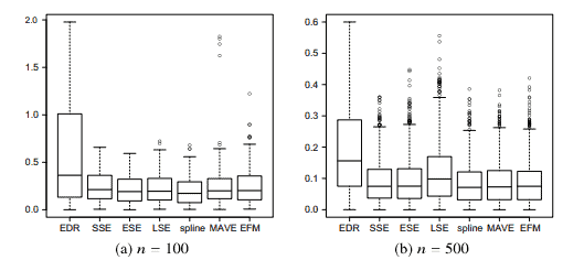
In this section, we compare the LSE with the Simple Score Estimator (SSE), the Efficient Score Estimator (ESE), the Effective Dimension Reduction (EDR) estimate, the spline estimate, the MAVE estimate, and the EFM estimate. We take part in the simulation settings in Balabdaoui et al. (2019a), which means that we take the dimension $d$ equal to 2 . Since the parameter belongs to the boundary of a circle in this case, we only have to determine a one-dimensional parameter. Using this fact, we use the parameterization $\alpha=\left(\alpha_{1}, \alpha_{2}\right)=(\cos (\beta), \sin (\beta))$ and determine the angle $\beta$ by a golden section search for the SSE, ESE, and spline estimate. For EDR, we used the $\mathrm{R}$ package edr: the method is discussed in Hristache et al. (2001). The spline method is described in Kuchibhotla and Patra (2020), and there exists an $R$ package simest for it, but we used our own implementation. For the MAVE method, we used the R package MAVE; for theory, see Xia (2006). For the EFM estimate (see Cui et al. 2011), we used an $\mathrm{R}$ script, due to Xia Cui and kindly provided to us by her and Rohit Patra. All runs of our simulations can be reproduced by running the $R$ scripts in Groeneboom $2018 .$

In simulation model 1 , we take $\alpha_{0}=(1 / \sqrt{2}, 1 / \sqrt{2})^{T}$ and $X=\left(X_{1}, X_{2}\right)^{T}$, where $X_{1}$ and $X_{2}$ are independent Uniform $(0,1)$ variables. The model is now
$$
Y=\psi_{0}\left(\alpha_{0}^{T} \boldsymbol{X}\right)+\varepsilon
$$
where $\psi_{0}(u)=u^{3}$ and $\varepsilon$ is a standard normal random variable, independent of $\boldsymbol{X}$.
In simulation model 2 , we also take $\alpha_{0}=(1 / \sqrt{2}, 1 / \sqrt{2})^{T}$ and $\boldsymbol{X}=\left(X_{1}, X_{2}\right)^{T}$, where $X_{1}$ and $X_{2}$ are independent Uniform $(0,1)$ variables. This time, however, the model is (Table 1)
$$
Y=\operatorname{Bin}\left(10, \exp \left(\boldsymbol{\alpha}{0}^{T} \boldsymbol{X}\right) /\left{1+\exp \left(\boldsymbol{\alpha}{0}^{T} \boldsymbol{X}\right)\right}\right)
$$
see also Table 2 in Balabdaoui et al. (2019a). This means $$
Y=\psi_{0}\left(\boldsymbol{\alpha}{0}^{T} \boldsymbol{X}\right)+\varepsilon $$ where $$ \psi{0}\left(\boldsymbol{\alpha}{0}^{T} \boldsymbol{X}\right)=10 \exp \left(\boldsymbol{\alpha}{0}^{T} \boldsymbol{X}\right) /\left{1+\exp \left(\boldsymbol{\alpha}{0}^{T} \boldsymbol{X}\right)\right}, \quad \varepsilon=N{n}-\psi_{0}\left(\boldsymbol{\alpha}{0}^{T} \boldsymbol{X}\right), $$ and $$ N{n}=\operatorname{Bin}\left(10, \frac{\exp \left(\boldsymbol{\alpha}{0}^{T} \boldsymbol{X}\right.}{1+\exp \left(\boldsymbol{\alpha}{0}^{T} \boldsymbol{X}\right)}\right)
$$
Note that indeed $\mathbb{E}{\varepsilon \mid \boldsymbol{X})=0$, but that we do not have independence of $\varepsilon$ and $\boldsymbol{X}$, as in the previous example.

商科代写|计量经济学代写Econometrics代考|Concluding Remarks

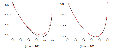
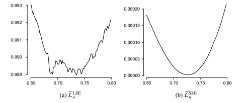
We replaced the “crossing of zero” estimators in Balabdaoui et al. (2019b) with profile least squares estimators. The asymptotic distribution of the estimators was determined and its behavior illustrated by a simulation study, using the same models as in Balabdaoui et al. (2019a).

In the first model, the error is independent of the covariate and homoscedastic and in this case, four of the estimators were efficient. In the other (binomial-logistic) model, the error was dependent on the covariates and not homoscedastic. It was shown that the Simple Score Estimate (SSE) had in fact a smaller asymptotic variance in this model than the other estimators for which the asymptotic variance is known, although the difference is very small and does not really show up in the simulations.
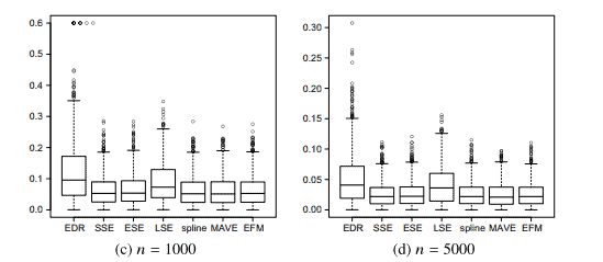
There is no uniformly best estimate in our simulation, but the EDR estimate is clearly inferior to the other estimates, including the LSE, in particular for the lower sample sizes. On the other hand, the LSE is inferior to the other estimators except for the EDR. All simulation results can be reproduced by running the $R$ scripts in Groeneboom (2018).

商科代写|计量经济学代写Econometrics代考|Mathematical Context

We assume to be given a sample $\mathscr{D}{n}=\left{\left(X{1}, Y_{1}\right), \ldots,\left(X_{n}, Y_{n}\right)\right}$ of i.i.d. observations, where each pair $\left(X_{i}, Y_{i}\right)$ takes values in $\mathscr{X} \times \mathscr{Y}$. Throughout, $\mathscr{X}$ is a Borel subset of $\mathbb{R}^{d}$, and $\mathscr{Y} \subset \mathbb{R}$ is either a finite set of labels (for classification) or a subset of $\mathbb{R}$ (for regression). The vector space $\mathbb{R}^{d}$ is endowed with the Euclidean norm $|\cdot|$.
Our goal is to construct a predictor $F: \mathscr{X} \rightarrow \mathbb{R}$ that assigns a response to each possible value of an independent random observation distributed as $X_{1}$. In the context of gradient boosting, this general problem is addressed by considering a class $\mathscr{F}$ of functions $f: \mathscr{X} \rightarrow \mathbb{R}$ (called the weak or base learners) and minimizing some empirical risk functional
$$
C_{n}(F)=\frac{1}{n} \sum_{i=1}^{n} \psi\left(F\left(X_{i}\right), Y_{i}\right)
$$
over the linear combinations of functions in $\mathscr{F}$. The function $\psi: \mathbb{R} \times \mathscr{Y} \rightarrow \mathbb{R}{+}$, called the loss, is convex in its first argument and measures the cost incurred by predicting $F\left(X{i}\right)$ when the answer is $Y_{i}$. For example, in the least squares regression problem, $\psi(x, y)=(y-x)^{2}$ and
$$
C_{n}(F)=\frac{1}{n} \sum_{i=1}^{n}\left(Y_{i}-F\left(X_{i}\right)\right)^{2} .
$$
However, many other examples are possible, as we will see below. Let $\delta_{z}$ denote the Dirac measure at $z$, and let $\mu_{n}=(1 / n) \sum_{i=1}^{n} \delta_{\left(X_{i}, Y_{j}\right)}$ be the empirical measure associated with the sample $\mathscr{D}{n}$. Clearly, $$ C{n}(F)=\mathbb{E} \psi(F(X), Y),
$$
where $(X, Y)$ denotes a random pair with distribution $\mu_{n}$ and the symbol $\mathbb{E}$ denotes the expectation with respect to $\mu_{n}$. Naturally, the theoretical (i.e., population) version of $C_{n}$ is
$$
C(F)=\mathbb{E} \psi\left(F\left(X_{1}\right), Y_{1}\right),
$$
where now the expectation is taken with respect to the distribution of $\left(X_{1}, Y_{1}\right)$. It turns out that most of our subsequent developments are independent of the context,whether empirical or theoretical. Therefore, to unify the notation, we let throughout $(X, Y)$ be a generic pair of random variables with distribution $\mu_{X, Y}$, keeping in mind that $\mu_{X, Y}$ may be the distribution of $\left(X_{1}, Y_{1}\right)$ (theoretical risk), the standard empirical measure $\mu_{n}$ (empirical risk), or any smoothed version of $\mu_{n}$.

商科代写|计量经济学代写Econometrics代考|ECON 7204

计量经济学代考

商科代写|计量经济学代写Econometrics代考|Simulation and Comparisons with Other Estimators

在本节中,我们将 LSE 与简单分数估计 (SSE)、有效分数估计 (ESE)、有效降维 (EDR) 估计、样条估计、MAVE 估计和 EFM 估计进行比较。我们参与了 Balabdaoui 等人的模拟设置。(2019a),这意味着我们取维度d等于 2 。由于在这种情况下参数属于圆的边界,我们只需要确定一个一维参数。利用这个事实,我们使用参数化一个=(一个1,一个2)=(因⁡(b),罪⁡(b))并确定角度b通过黄金分割搜索 SSE、ESE 和样条估计。对于 EDR,我们使用Rpackage edr:Hristache 等人讨论了该方法。(2001 年)。样条方法在 Kuchibhotla 和 Patra (2020) 中有描述,并且存在R最适合它的包,但我们使用了自己的实现。对于 MAVE 方法,我们使用了 R 包 MAVE;理论见Xia (2006)。对于 EFM 估计(参见 Cui et al. 2011),我们使用了R剧本,感谢夏翠,由她和 Rohit Patra 提供给我们。我们模拟的所有运行都可以通过运行RGroeneboom 中的脚本2018.

在仿真模型 1 中,我们取一个0=(1/2,1/2)吨和X=(X1,X2)吨, 在哪里X1和X2是独立的制服(0,1)变量。模型现在

是=ψ0(一个0吨X)+e
在哪里ψ0(在)=在3和e是标准正态随机变量,独立于X.
在仿真模型 2 中,我们还取一个0=(1/2,1/2)吨和X=(X1,X2)吨, 在哪里X1和X2是独立的制服(0,1)变量。然而,这一次,模型是(表 1)

Y=\operatorname{Bin}\left(10, \exp \left(\boldsymbol{\alpha}{0}^{T} \boldsymbol{X}\right) /\left{1+\exp \left(\粗体符号{\alpha}{0}^{T} \boldsymbol{X}\right)\right}\right)Y=\operatorname{Bin}\left(10, \exp \left(\boldsymbol{\alpha}{0}^{T} \boldsymbol{X}\right) /\left{1+\exp \left(\粗体符号{\alpha}{0}^{T} \boldsymbol{X}\right)\right}\right)
另见 Balabdaoui 等人的表 2。(2019a)。这表示

是=ψ0(一个0吨X)+e在哪里

\psi{0}\left(\boldsymbol{\alpha}{0}^{T} \boldsymbol{X}\right)=10 \exp \left(\boldsymbol{\alpha}{0}^{T} \ boldsymbol{X}\right) /\left{1+\exp \left(\boldsymbol{\alpha}{0}^{T} \boldsymbol{X}\right)\right}, \quad \varepsilon=N{ n}-\psi_{0}\left(\boldsymbol{\alpha}{0}^{T} \boldsymbol{X}\right),\psi{0}\left(\boldsymbol{\alpha}{0}^{T} \boldsymbol{X}\right)=10 \exp \left(\boldsymbol{\alpha}{0}^{T} \ boldsymbol{X}\right) /\left{1+\exp \left(\boldsymbol{\alpha}{0}^{T} \boldsymbol{X}\right)\right}, \quad \varepsilon=N{ n}-\psi_{0}\left(\boldsymbol{\alpha}{0}^{T} \boldsymbol{X}\right),和

ñn=垃圾桶⁡(10,经验⁡(一个0吨X1+经验⁡(一个0吨X))
注意确实 $\mathbb{E}{\varepsilon \mid \boldsymbol{X})=0,b在吨吨H一个吨在和d○n○吨H一个在和一世nd和p和nd和nC和○F\伐普西隆一个nd\boldsymbol{X}$,如上例所示。

商科代写|计量经济学代写Econometrics代考|Concluding Remarks

我们替换了 Balabdaoui 等人的“过零”估计量。(2019b)具有轮廓最小二乘估计器。使用与 Balabdaoui 等人相同的模型,确定了估计量的渐近分布,并通过模拟研究说明了其行为。(2019a)。

在第一个模型中,误差与协变量和同方差无关,在这种情况下,四个估计量是有效的。在另一个(二项式逻辑)模型中,误差取决于协变量而不是同方差。结果表明,与已知渐近方差的其他估计量相比,简单分数估计 (SSE) 实际上在该模型中具有更小的渐近方差,尽管差异非常小并且并未真正显示在模拟中。
在我们的模拟中没有统一的最佳估计,但 EDR 估计明显不如其他估计,包括 LSE,特别是对于较小的样本量。另一方面,LSE 不如 EDR 以外的其他估计量。所有模拟结果都可以通过运行RGroeneboom (2018) 中的脚本。

商科代写|计量经济学代写Econometrics代考|Mathematical Context

我们假设给定一个样本\mathscr{D}{n}=\left{\left(X{1}, Y_{1}\right), \ldots,\left(X_{n}, Y_{n}\right)\right}\mathscr{D}{n}=\left{\left(X{1}, Y_{1}\right), \ldots,\left(X_{n}, Y_{n}\right)\right}独立同分布观察,其中每一对(X一世,是一世)取值X×是. 始终,X是一个 Borel 子集Rd, 和是⊂R是一组有限的标签(用于分类)或R(用于回归)。向量空间Rd被赋予欧几里得范数|⋅|.
我们的目标是构建一个预测器F:X→R将响应分配给独立随机观察的每个可能值,分布为X1. 在梯度提升的背景下,这个一般问题是通过考虑一个类来解决的F功能F:X→R(称为弱学习器或基础学习器)并最小化一些经验风险函数

Cn(F)=1n∑一世=1nψ(F(X一世),是一世)
在函数的线性组合上F. 功能ψ:R×是→R+,称为损失,在其第一个参数中是凸的,并衡量通过预测所产生的成本F(X一世)当答案是是一世. 例如,在最小二乘回归问题中,ψ(X,是)=(是−X)2和

Cn(F)=1n∑一世=1n(是一世−F(X一世))2.
但是,许多其他示例也是可能的,我们将在下面看到。让d和表示狄拉克测度和, 然后让μn=(1/n)∑一世=1nd(X一世,是j)是与样本相关的经验度量Dn. 清楚地,

Cn(F)=和ψ(F(X),是),
在哪里(X,是)表示具有分布的随机对μn和符号和表示相对于的期望μn. 自然地,理论(即人口)版本Cn是

C(F)=和ψ(F(X1),是1),
现在的期望是关于分布的(X1,是1). 事实证明,我们随后的大部分发展都独立于背景,无论是经验的还是理论的。因此,为了统一符号,我们让通篇(X,是)是具有分布的通用随机变量对μX,是,请记住μX,是可能是分布(X1,是1)(理论风险),标准经验测量μn(经验风险),或任何平滑版本μn.

商科代写|计量经济学代写Econometrics代考 请认准statistics-lab™

统计代写请认准statistics-lab™. statistics-lab™为您的留学生涯保驾护航。

金融工程代写

金融工程是使用数学技术来解决金融问题。金融工程使用计算机科学、统计学、经济学和应用数学领域的工具和知识来解决当前的金融问题,以及设计新的和创新的金融产品。

非参数统计代写

非参数统计指的是一种统计方法,其中不假设数据来自于由少数参数决定的规定模型;这种模型的例子包括正态分布模型和线性回归模型。

广义线性模型代考

广义线性模型(GLM)归属统计学领域,是一种应用灵活的线性回归模型。该模型允许因变量的偏差分布有除了正态分布之外的其它分布。

术语 广义线性模型(GLM)通常是指给定连续和/或分类预测因素的连续响应变量的常规线性回归模型。它包括多元线性回归,以及方差分析和方差分析(仅含固定效应)。

有限元方法代写

有限元方法(FEM)是一种流行的方法,用于数值解决工程和数学建模中出现的微分方程。典型的问题领域包括结构分析、传热、流体流动、质量运输和电磁势等传统领域。

有限元是一种通用的数值方法,用于解决两个或三个空间变量的偏微分方程(即一些边界值问题)。为了解决一个问题,有限元将一个大系统细分为更小、更简单的部分,称为有限元。这是通过在空间维度上的特定空间离散化来实现的,它是通过构建对象的网格来实现的:用于求解的数值域,它有有限数量的点。边界值问题的有限元方法表述最终导致一个代数方程组。该方法在域上对未知函数进行逼近。[1] 然后将模拟这些有限元的简单方程组合成一个更大的方程系统,以模拟整个问题。然后,有限元通过变化微积分使相关的误差函数最小化来逼近一个解决方案。

tatistics-lab作为专业的留学生服务机构,多年来已为美国、英国、加拿大、澳洲等留学热门地的学生提供专业的学术服务,包括但不限于Essay代写,Assignment代写,Dissertation代写,Report代写,小组作业代写,Proposal代写,Paper代写,Presentation代写,计算机作业代写,论文修改和润色,网课代做,exam代考等等。写作范围涵盖高中,本科,研究生等海外留学全阶段,辐射金融,经济学,会计学,审计学,管理学等全球99%专业科目。写作团队既有专业英语母语作者,也有海外名校硕博留学生,每位写作老师都拥有过硬的语言能力,专业的学科背景和学术写作经验。我们承诺100%原创,100%专业,100%准时,100%满意。

随机分析代写


随机微积分是数学的一个分支,对随机过程进行操作。它允许为随机过程的积分定义一个关于随机过程的一致的积分理论。这个领域是由日本数学家伊藤清在第二次世界大战期间创建并开始的。

时间序列分析代写

随机过程,是依赖于参数的一组随机变量的全体,参数通常是时间。 随机变量是随机现象的数量表现,其时间序列是一组按照时间发生先后顺序进行排列的数据点序列。通常一组时间序列的时间间隔为一恒定值(如1秒,5分钟,12小时,7天,1年),因此时间序列可以作为离散时间数据进行分析处理。研究时间序列数据的意义在于现实中,往往需要研究某个事物其随时间发展变化的规律。这就需要通过研究该事物过去发展的历史记录,以得到其自身发展的规律。

回归分析代写

多元回归分析渐进(Multiple Regression Analysis Asymptotics)属于计量经济学领域,主要是一种数学上的统计分析方法,可以分析复杂情况下各影响因素的数学关系,在自然科学、社会和经济学等多个领域内应用广泛。

MATLAB代写

MATLAB 是一种用于技术计算的高性能语言。它将计算、可视化和编程集成在一个易于使用的环境中,其中问题和解决方案以熟悉的数学符号表示。典型用途包括:数学和计算算法开发建模、仿真和原型制作数据分析、探索和可视化科学和工程图形应用程序开发,包括图形用户界面构建MATLAB 是一个交互式系统,其基本数据元素是一个不需要维度的数组。这使您可以解决许多技术计算问题,尤其是那些具有矩阵和向量公式的问题,而只需用 C 或 Fortran 等标量非交互式语言编写程序所需的时间的一小部分。MATLAB 名称代表矩阵实验室。MATLAB 最初的编写目的是提供对由 LINPACK 和 EISPACK 项目开发的矩阵软件的轻松访问,这两个项目共同代表了矩阵计算软件的最新技术。MATLAB 经过多年的发展,得到了许多用户的投入。在大学环境中,它是数学、工程和科学入门和高级课程的标准教学工具。在工业领域,MATLAB 是高效研究、开发和分析的首选工具。MATLAB 具有一系列称为工具箱的特定于应用程序的解决方案。对于大多数 MATLAB 用户来说非常重要,工具箱允许您学习应用专业技术。工具箱是 MATLAB 函数(M 文件)的综合集合,可扩展 MATLAB 环境以解决特定类别的问题。可用工具箱的领域包括信号处理、控制系统、神经网络、模糊逻辑、小波、仿真等。

R语言代写问卷设计与分析代写
PYTHON代写回归分析与线性模型代写
MATLAB代写方差分析与试验设计代写
STATA代写机器学习/统计学习代写
SPSS代写计量经济学代写
EVIEWS代写时间序列分析代写
EXCEL代写深度学习代写
SQL代写各种数据建模与可视化代写

商科代写|计量经济学代写Econometrics代考|ECOM20001

如果你也在 怎样代写计量经济学Econometrics这个学科遇到相关的难题,请随时右上角联系我们的24/7代写客服。

计量经济学,对经济关系的统计和数学分析,通常作为经济预测的基础。这种信息有时被政府用来制定经济政策,也被私人企业用来帮助价格、库存和生产方面的决策。

statistics-lab™ 为您的留学生涯保驾护航 在代写计量经济学Econometrics方面已经树立了自己的口碑, 保证靠谱, 高质且原创的统计Statistics代写服务。我们的专家在代写计量经济学Econometrics代写方面经验极为丰富,各种代写计量经济学Econometrics相关的作业也就用不着说。

我们提供的计量经济学Econometrics及其相关学科的代写,服务范围广, 其中包括但不限于:

  • Statistical Inference 统计推断
  • Statistical Computing 统计计算
  • Advanced Probability Theory 高等概率论
  • Advanced Mathematical Statistics 高等数理统计学
  • (Generalized) Linear Models 广义线性模型
  • Statistical Machine Learning 统计机器学习
  • Longitudinal Data Analysis 纵向数据分析
  • Foundations of Data Science 数据科学基础
商科代写|计量经济学代写Econometrics代考|ECOM20001

商科代写|计量经济学代写Econometrics代考|General Conditions and the Functions ψˆ n,αˆ and ψα

We give general conditions that we assume to hold in the remainder of the paper here and give graphical comparisons of the functions $\hat{\psi}{n, \alpha}$ and $\psi{\alpha}$, where $\psi_{\alpha}$ is defined in Definition $1 .$

Example 1 As an illustrative example, we take $d=2, \psi_{0}(x)=x^{3}, \alpha_{0}=(1 / \sqrt{2}$, $1 / \sqrt{2})^{T}, Y_{i}=\psi_{0}\left(\alpha_{0}^{T} X_{i}\right)+\varepsilon_{i}$, where the $\varepsilon_{i}$ are i.i.d. standard normal random variables, independent of the $\boldsymbol{X}{i}$, which are i.i.d. random vectors, consisting of two independent Uniform $(0,1)$ random variables. In this case, the conditional expectation function (5) is a rather complicated function of $\alpha$ which we shall not give here but can be computed by a computer package such as Mathematica or Maple. The loss functions: $L^{\mathrm{LSE}}: \alpha{1} \mapsto \mathbb{E}\left{Y-\psi_{\alpha}\left(\alpha^{T} \boldsymbol{X}\right)\right}^{2} \quad$ and $\quad \widehat{L}{n}^{\mathrm{LSE}}: \alpha{1} \mapsto n^{-1} \sum_{i=1}^{n}\left{Y_{i}-\hat{\psi}{n, \alpha}\left(\alpha^{T} \boldsymbol{X}{i}\right)\right}^{2}$
where the loss function $\widehat{L}{n}^{L S E}$ is for sample sizes $n=10,000$ and $n=100,000$, and $\alpha=\left(\alpha{1}, \alpha_{2}\right)^{T}$. For $\alpha_{1} \in[0,1]$ and $\alpha_{2}$ equal to the positive root $\left{1-\alpha_{1}^{2}\right}^{1 / 2}$, we get Fig. 1. The function $L^{\mathrm{LSE}}$ has a minimum equal to 1 at $\alpha_{1}=1 / \sqrt{2}$, and $\widehat{L}{n}^{\mathrm{LSE}}$ has a minimum at a value very close to $1 / \sqrt{2}$ (furnishing the profile LSE $\hat{\alpha}{n}$ ), which gives a visual evidence for consistency of the profile LSE.

In order to show the $\sqrt{n}$-consistency and asymptotic normality of the estimators in the next sections, we now introduce some conditions, which correspond to those in Balabdaoui et al. (2019b). We note that we do not need conditions on reparameterization.
(A1) $\boldsymbol{X}$ has a density w.r.t. Lebesgue measure on its support $\mathcal{X}$, which is a convex set $\mathcal{X}$ with a nonempty interior, and satisfies $\mathcal{X} \subset\left{x \in \mathbb{R}^{d}:|x| \leq R\right}$ for some $R>0$.
(A2) The function $\psi_{0}$ is bounded on the set $\left{u \in \mathbb{R}: u=\alpha_{0}^{T} \boldsymbol{x}, \boldsymbol{x} \in \mathcal{X}\right}$.
(A3) There exists $\delta>0$ such that the conditional expectation $\tilde{\psi}{\alpha}$, defined by (5), is nondecreasing on $I{\alpha}=\left{u \in \mathbb{R}: u=\alpha^{T} \boldsymbol{x}, x \in \mathcal{X}\right}$ and satisfies $\bar{\psi}{\alpha}=\psi{\alpha}$, so minimizes $$
\left|\mathbb{E}\left{Y-\psi\left(\boldsymbol{\alpha}^{T} \boldsymbol{X}\right)\right} \boldsymbol{X}\right|^{2}
$$
over nondecreasing functions $\psi$, if $\left|\boldsymbol{\alpha}-\boldsymbol{\alpha}_{0}\right| \leq \delta$.

商科代写|计量经济学代写Econometrics代考|The Limit Theory for the SSE

In this section, we derive the limit distribution of the SSE introduced above. In our derivation, the function $\psi_{\alpha}$ of Definition 1 plays a crucial role. Below, we will use the following assumptions, additionally to $(\mathrm{A} 1)-(\mathrm{A} 6)$.
(A7) There exists a $\delta>0$ such that for all $\alpha \in\left(\mathcal{B}\left(\alpha_{0}, \delta\right) \cap \mathcal{S}{d-1}\right) \backslash\left{\alpha{0}\right}$, the random variable
$$
\operatorname{cov}\left(\left(\boldsymbol{\alpha}{0}-\boldsymbol{\alpha}\right)^{T} \boldsymbol{X}, \psi{0}\left(\boldsymbol{\alpha}{0}^{T} \boldsymbol{X}\right) \mid \boldsymbol{\alpha}^{T} \boldsymbol{X}\right) $$ is not equal to 0 almost surely. (A8) The matrix $$ \mathbb{E}\left[\psi{0}^{\prime}\left(\boldsymbol{\alpha}{0}^{T} \boldsymbol{X}\right) \operatorname{cov}\left(\boldsymbol{X} \mid \boldsymbol{\alpha}{0}^{T} \boldsymbol{X}\right)\right]
$$
has rank $d-1$.
We start by comparing (3) with the function
$$
\alpha \mapsto\left|\mathbb{E}\left{Y-\psi_{\alpha}\left(\alpha^{T} \boldsymbol{X}\right)\right} \boldsymbol{X}\right|^{2}
$$ As in Sect. 1, the function $\hat{\psi}_{n, \alpha}$ is just the (isotonic) least squares estimate for fixed $\alpha$.

商科代写|计量经济学代写Econometrics代考|The Limit Theory for ESE and Cubic Spline Estimator

The proofs of the consistency and asymptotic normality of the ESE and spline estimator are highly similar to the proofs of these facts for the SSE in the preceding section. The only extra ingredient is the occurrence of the estimate of the derivative of the link function. We only discuss the asymptotic normality.
In addition to the assumptions (A1)-(A7), we now assume the following:
(A8′) $\psi_{\alpha}$ is twice differentiable on $\left.\inf {x \in \mathcal{X}}\left(\alpha^{T} \boldsymbol{x}\right), \sup {x \in \mathcal{X}^{\prime}}\left(\boldsymbol{\alpha}^{T} \boldsymbol{x}\right)\right)$.
(A9) The matrix
$$
\mathbb{E}\left[\psi_{0}^{\prime}\left(\alpha_{0}^{T} \boldsymbol{X}\right)^{2} \operatorname{cov}\left(\boldsymbol{X} \mid \alpha_{0}^{T} \boldsymbol{X}\right)\right]
$$
has rank $d-1$.
An essential step is again to show that
$$
\begin{aligned}
&\int \boldsymbol{x}\left{y-\hat{\psi}{n, \hat{\alpha}{n}}\left(\hat{\boldsymbol{\alpha}}{n}^{T} \boldsymbol{x}\right)\right} \hat{\psi}{n \hat{\boldsymbol{\alpha}}{n}}^{\prime}\left(\hat{\boldsymbol{\alpha}}{n}^{T} \boldsymbol{x}\right) d \mathbb{P}{n}(\boldsymbol{x}, y) \ &=\int\left{\boldsymbol{x}-\mathbb{E}\left(X \mid \hat{\boldsymbol{\alpha}}{n}^{T} \boldsymbol{X}\right)\right}\left{y-\hat{\psi}{n, \hat{\alpha}{n}}\left(\hat{\boldsymbol{\alpha}}{n}^{T} \boldsymbol{x}\right)\right} \hat{\psi}{n \hat{\alpha}{n}}^{\prime}\left(\hat{\alpha}{n}^{T} \boldsymbol{x}\right) d \mathbb{P}{n}(\boldsymbol{x}, y) \ &+o{p}\left(n^{-1 / 2}\right)+o_{p}\left(\hat{\alpha}{n}-\boldsymbol{\alpha}{0}\right)
\end{aligned}
$$
For the ESE, this is done by defining the piecewise constant function $\bar{\rho}{n, \alpha}$ for $u$ in the interval between successive jumps $\tau{i}$ and $\tau_{i+1}$ ) of $\hat{\psi}{n \alpha}$ by $$ \bar{\rho}{n, \alpha}(u)= \begin{cases}\mathbb{E}\left[\boldsymbol{X} \mid \alpha^{T} \boldsymbol{X}=\tau_{i}\right] \psi_{\alpha}^{\prime}\left(\tau_{i}\right) & \text { if } \psi_{\alpha}(u)>\hat{\psi}{n \alpha}\left(\tau{i}\right) \text { for all } u \in\left(\tau_{i}, \tau_{i+1}\right) \ \mathbb{E}\left[\boldsymbol{X} \mid \alpha^{T} \boldsymbol{X}=s\right] \psi_{\alpha}^{\prime}(s) & \text { if } \psi_{\alpha}(s)=\hat{\psi}{n \alpha}(s) \text { for some } s \in\left(\tau{i}, \tau_{i+1}\right) \ \mathbb{E}\left[\boldsymbol{X} \mid \alpha^{T} \boldsymbol{X}=\tau_{i+1}\right] \psi_{\alpha}^{\prime}\left(\tau_{i+1}\right) & \text { if } \psi_{\alpha}(u)<\hat{\psi}{n \alpha}\left(\tau{i}\right) \text { for all } u \in\left(\tau_{i}, \tau_{i+1}\right)\end{cases}
$$ see Appendix E in the supplement of Balabdaoui et al. (2019b). The remaining part of the proof runs along the same lines as the proof for the SSE. For additional details, see Appendix E in the supplement of Balabdaoui et al. (2019b).

The corresponding step in the proof for the spline estimator is given by the following lemma.

商科代写|计量经济学代写Econometrics代考|ECOM20001

计量经济学代考

商科代写|计量经济学代写Econometrics代考|General Conditions and the Functions ψˆ n,αˆ and ψα

我们给出了我们假设在本文的其余部分中持有的一般条件,并给出了函数的图形比较 $\hat{\psi}, \alpha, \alpha$ 和 $\psi \alpha$ ,在哪里 $\psi_{\alpha}$ 在 定义中定义 1 .
例 1 作为一个说明性的例子,我们取 $d=2, \psi_{0}(x)=x^{3}, \alpha_{0}=(1 / \sqrt{2}, 1 / \sqrt{2})^{T}, Y_{i}=\psi_{0}\left(\alpha_{0}^{T} X_{i}\right)+\varepsilon_{i}$ , 其中 $\varepsilon_{i}$ 是独立同分布的标准正态随机变量,独立于 $\boldsymbol{X} i$ ,它们是 iid 随机向量,由两个独立的 Uniform 组成 $(0,1)$ 随机变量。在这种情况下,条件期望函数 (5) 是一个相当复杂的函数 $\alpha$ 我们不会在这里给出,但可以通过诸如 Mathematica 或 Maple 之类的计算机包来计算。损失函数: 和
$\mathrm{~ I q u a d ~ I w i d e h a t { { \ { n }}$ 其中损失函数 $\widehat{L} n^{L S E}$ 适用于样本量 $n=10,000$ 和 $n=100,000$ ,和 $\alpha=\left(\alpha 1, \alpha_{2}\right)^{T}$. 为了 $\alpha_{1} \in[0,1]$ 和 $\alpha_{2}$ 等于正根 $\mathrm{~ l e f t { 1 – l a l p h a _ { 1 } へ { 2 } \ r i g h t }}$ $\widehat{L} n^{\mathrm{LSE}}$ 最小值非常接近 $1 / \sqrt{2}$ (提供简介 LSE $\left.\hat{\alpha} n\right)$ ,这为配置文件 LSE 的一致性提供了视觉证据。
为了显示 $\sqrt{n}$-在下一节中估计量的一致性和渐近正态性,我们现在介绍一些条件,这些条件对应于 Balabdaoui 等 人的条件。(2019b)。我们注意到我们不需要重新参数化的条件。
(A1) $\boldsymbol{X}$ 在其支持上有一个密度 wrt Lebesgue 度量 $\mathcal{X}$ ,这是一个凸集 $\mathcal{X}$ 具有非空的内部,并且满足
$\mathrm{~ I m a t h c a l { X } }}$
(A2) 功能 $\psi_{0}$ 有界在集合上
\eft ${u \backslash$ in $\backslash \mathrm{~ m a t h b b b { R } : ~ u =}$
(A3) 存在 $\delta>0$ 使得条件期望 $\tilde{\psi} \alpha$ ,由 (5) 定义,在
I{\alpha $}=\backslash 1$ eft $\left{u \backslash\right.$ in $\backslash$ mathbb ${R}: u=\backslash a \mid p h a^{\wedge}{T} \backslash$ boldsymbol ${x}, x \backslash \mathrm{~ i n ~}$
Veft $\backslash \backslash$ mathbb ${$ E $} \backslash$ eft ${Y \mathrm{~ – ~ \ p s i V l e f t (}$
过非减函数 $\psi$ ,如果 $\left|\boldsymbol{\alpha}-\boldsymbol{\alpha}_{0}\right| \leq \delta$.

商科代写|计量经济学代写Econometrics代考|The Limit Theory for the SSE

在本节中,我们推导出上面介绍的 SSE 的极限分布。在我们的推导中,函数 $\psi_{\alpha}$ 定义 1 起着至关重要的作用。下 面,我们将使用以下假设,此外 $(\mathrm{A} 1)-(\mathrm{A} 6)$.
(A7) 存在一个 $\delta>0$ 这样对于所有人
$\mathrm{~ \ a l p h a ~ \ i n \ l e f t ( \ m a t h c a l { B }}$
变量
$$
\operatorname{cov}\left((\boldsymbol{\alpha} 0-\boldsymbol{\alpha})^{T} \boldsymbol{X}, \psi 0\left(\boldsymbol{\alpha} 0^{T} \boldsymbol{X}\right) \mid \boldsymbol{\alpha}^{T} \boldsymbol{X}\right)
$$
几乎肯定不等于 0 。 (A8) 矩阵
$$
\mathbb{E}\left[\psi 0^{\prime}\left(\boldsymbol{\alpha} 0^{T} \boldsymbol{X}\right) \operatorname{cov}\left(\boldsymbol{X} \mid \boldsymbol{\alpha} 0^{T} \boldsymbol{X}\right)\right]
$$
有等级 $d-1$.
我们首先将 (3) 与函数进行比较
\alpha \mapsto\left } \backslash \backslash \text { mathbb } { E } \backslash l e f t { Y \mathrm { ~ –
就像在教派中一样。1、功能 $\hat{\psi}_{n, \alpha}$ 只是固定的 (等渗的) 最小二乘估计 $\alpha$.

商科代写|计量经济学代写Econometrics代考|The Limit Theory for ESE and Cubic Spline Estimator

ESE 和样条估计量的一致性和渐近正态性的证明与上一节中 SSE 的这些事实的证明非常相似。唯一的额外因素是链 接函数导数估计的出现。我们只讨论渐近正态性。
除了假设(A1 ) – (A7),我们现在假设以下:
(A8′) $\psi_{\alpha}$ 是两次可微的 $\left.\inf x \in \mathcal{X}\left(\alpha^{T} \boldsymbol{x}\right), \sup x \in \mathcal{X}^{\prime}\left(\boldsymbol{\alpha}^{T} \boldsymbol{x}\right)\right)$.
(A9) 矩阵
$$
\mathbb{E}\left[\psi_{0}^{\prime}\left(\alpha_{0}^{T} \boldsymbol{X}\right)^{2} \operatorname{cov}\left(\boldsymbol{X} \mid \alpha_{0}^{T} \boldsymbol{X}\right)\right]
$$
有等级 $d-1$.
一个重要的步骙是再次证明
\begin } { \text { 对齐 } } \text { \& Int } \backslash \text { boldsymbol } { x } \backslash l e f t { y \mathrm { ~ – ~
对于 ESE,这是通过定义分段常数函数来完成的 $\bar{\rho} n, \alpha$ 为了 $u$ 在连续咷跃之间的间隔 $\tau i$ 和 $\tau_{i+1} )$ 的 $\hat{\psi} n \alpha$ 经过 $\bar{\rho} n, \alpha(u)=\left{\mathbb{E}\left[\boldsymbol{X} \mid \alpha^{T} \boldsymbol{X}=\tau_{i}\right] \psi_{\alpha}^{\prime}\left(\tau_{i}\right) \quad\right.$ if $\psi_{\alpha}(u)>\hat{\psi} n \alpha(\tau i)$ for all $u \in\left(\tau_{i}, \tau_{i+1}\right) \mathbb{E}\left[\boldsymbol{X} \mid \alpha^{T} \boldsymbol{X}=s\right.$ 请参阅 Balabdaoui 等人的补充资料中的附录 $E_{。}$ (2019b) 。证明的其余部分与 SSE 的证明相同。有关详细信 息,请参阅 Balabdaoui 等人的补充资料中的附录 $E_{0}$ (2019b)。
样条估计器证明中的相应步骙由以下引理给出。

商科代写|计量经济学代写Econometrics代考 请认准statistics-lab™

统计代写请认准statistics-lab™. statistics-lab™为您的留学生涯保驾护航。

金融工程代写

金融工程是使用数学技术来解决金融问题。金融工程使用计算机科学、统计学、经济学和应用数学领域的工具和知识来解决当前的金融问题,以及设计新的和创新的金融产品。

非参数统计代写

非参数统计指的是一种统计方法,其中不假设数据来自于由少数参数决定的规定模型;这种模型的例子包括正态分布模型和线性回归模型。

广义线性模型代考

广义线性模型(GLM)归属统计学领域,是一种应用灵活的线性回归模型。该模型允许因变量的偏差分布有除了正态分布之外的其它分布。

术语 广义线性模型(GLM)通常是指给定连续和/或分类预测因素的连续响应变量的常规线性回归模型。它包括多元线性回归,以及方差分析和方差分析(仅含固定效应)。

有限元方法代写

有限元方法(FEM)是一种流行的方法,用于数值解决工程和数学建模中出现的微分方程。典型的问题领域包括结构分析、传热、流体流动、质量运输和电磁势等传统领域。

有限元是一种通用的数值方法,用于解决两个或三个空间变量的偏微分方程(即一些边界值问题)。为了解决一个问题,有限元将一个大系统细分为更小、更简单的部分,称为有限元。这是通过在空间维度上的特定空间离散化来实现的,它是通过构建对象的网格来实现的:用于求解的数值域,它有有限数量的点。边界值问题的有限元方法表述最终导致一个代数方程组。该方法在域上对未知函数进行逼近。[1] 然后将模拟这些有限元的简单方程组合成一个更大的方程系统,以模拟整个问题。然后,有限元通过变化微积分使相关的误差函数最小化来逼近一个解决方案。

tatistics-lab作为专业的留学生服务机构,多年来已为美国、英国、加拿大、澳洲等留学热门地的学生提供专业的学术服务,包括但不限于Essay代写,Assignment代写,Dissertation代写,Report代写,小组作业代写,Proposal代写,Paper代写,Presentation代写,计算机作业代写,论文修改和润色,网课代做,exam代考等等。写作范围涵盖高中,本科,研究生等海外留学全阶段,辐射金融,经济学,会计学,审计学,管理学等全球99%专业科目。写作团队既有专业英语母语作者,也有海外名校硕博留学生,每位写作老师都拥有过硬的语言能力,专业的学科背景和学术写作经验。我们承诺100%原创,100%专业,100%准时,100%满意。

随机分析代写


随机微积分是数学的一个分支,对随机过程进行操作。它允许为随机过程的积分定义一个关于随机过程的一致的积分理论。这个领域是由日本数学家伊藤清在第二次世界大战期间创建并开始的。

时间序列分析代写

随机过程,是依赖于参数的一组随机变量的全体,参数通常是时间。 随机变量是随机现象的数量表现,其时间序列是一组按照时间发生先后顺序进行排列的数据点序列。通常一组时间序列的时间间隔为一恒定值(如1秒,5分钟,12小时,7天,1年),因此时间序列可以作为离散时间数据进行分析处理。研究时间序列数据的意义在于现实中,往往需要研究某个事物其随时间发展变化的规律。这就需要通过研究该事物过去发展的历史记录,以得到其自身发展的规律。

回归分析代写

多元回归分析渐进(Multiple Regression Analysis Asymptotics)属于计量经济学领域,主要是一种数学上的统计分析方法,可以分析复杂情况下各影响因素的数学关系,在自然科学、社会和经济学等多个领域内应用广泛。

MATLAB代写

MATLAB 是一种用于技术计算的高性能语言。它将计算、可视化和编程集成在一个易于使用的环境中,其中问题和解决方案以熟悉的数学符号表示。典型用途包括:数学和计算算法开发建模、仿真和原型制作数据分析、探索和可视化科学和工程图形应用程序开发,包括图形用户界面构建MATLAB 是一个交互式系统,其基本数据元素是一个不需要维度的数组。这使您可以解决许多技术计算问题,尤其是那些具有矩阵和向量公式的问题,而只需用 C 或 Fortran 等标量非交互式语言编写程序所需的时间的一小部分。MATLAB 名称代表矩阵实验室。MATLAB 最初的编写目的是提供对由 LINPACK 和 EISPACK 项目开发的矩阵软件的轻松访问,这两个项目共同代表了矩阵计算软件的最新技术。MATLAB 经过多年的发展,得到了许多用户的投入。在大学环境中,它是数学、工程和科学入门和高级课程的标准教学工具。在工业领域,MATLAB 是高效研究、开发和分析的首选工具。MATLAB 具有一系列称为工具箱的特定于应用程序的解决方案。对于大多数 MATLAB 用户来说非常重要,工具箱允许您学习应用专业技术。工具箱是 MATLAB 函数(M 文件)的综合集合,可扩展 MATLAB 环境以解决特定类别的问题。可用工具箱的领域包括信号处理、控制系统、神经网络、模糊逻辑、小波、仿真等。

R语言代写问卷设计与分析代写
PYTHON代写回归分析与线性模型代写
MATLAB代写方差分析与试验设计代写
STATA代写机器学习/统计学习代写
SPSS代写计量经济学代写
EVIEWS代写时间序列分析代写
EXCEL代写深度学习代写
SQL代写各种数据建模与可视化代写

商科代写|商业建模代写Business Modeling代考|INFS6016

如果你也在 怎样代写商业建模Business Modeling这个学科遇到相关的难题,请随时右上角联系我们的24/7代写客服。

商业建模是一种风格化的模式,描述了公司如何创造并向客户提供价值,以及他们如何为此获得回报。

statistics-lab™ 为您的留学生涯保驾护航 在代写商业建模Business Modeling方面已经树立了自己的口碑, 保证靠谱, 高质且原创的统计Statistics代写服务。我们的专家在代写商业建模Business Modeling代写方面经验极为丰富,各种代写商业建模Business Modeling相关的作业也就用不着说。

我们提供的商业建模Business Modeling及其相关学科的代写,服务范围广, 其中包括但不限于:

  • Statistical Inference 统计推断
  • Statistical Computing 统计计算
  • Advanced Probability Theory 高等概率论
  • Advanced Mathematical Statistics 高等数理统计学
  • (Generalized) Linear Models 广义线性模型
  • Statistical Machine Learning 统计机器学习
  • Longitudinal Data Analysis 纵向数据分析
  • Foundations of Data Science 数据科学基础
商科代写|商业建模代写Business Modeling代考|INFS6016

商科代写|商业建模代写Business Modeling代考|Process Flow

When we look at the work of Shigeo Shingo about improvement of production processes, he is not talking about processes as such, but rather at process delays. Essentially, he is discussing lossless transitions between (sub)processes and reduction of avoidable waste in transformation (sub)processes [6]. Any storage that is not required for stabilisation of the product is considered a process delay, and as such a loss to be avoided. However, when the period between order and delivery is shorter than the actual time it takes to manufacture a product, stocks are necessary. Therefore, reduction of process delay is key to Shingo’s thinking. Faster production throughput implies less need for stocks, and shifts production from push to pull.

Process improvement is fundamentally about time and timing. Underutilisation of production capacity is allowed when it reduces significantly throughput time. As an example, imagine a production company where the packaging is the bottleneck. The company has to find a balance between order lead time, customer service levels, idle time of expensive packaging equipment, and scrapped stock waiting for orders that did not materialise. Considerations of production cost would argue against investments in equipment, market considerations would argue against higher lead times. Taiichi Ohno writes “In production, ‘waste’ refers to all elements of production that only increase cost without adding value – for example, excess people, inventory, and equipment” [7]. The company will have to balance excess equipment against excess stocks. “Idle equipment” cannot always be equated to “excess equipment”.

To summarise, this kind of process thinking is primarily about pull, flow and avoidance of delays. This requires balancing on both the design level (production capacities) and the operational level (mechanisms for mutual adjustment/modification of production capacities). Processes can be recognised on different aggregation levels. They can be continuous or discrete. To realise flow through processes mechanisms must be in place that prevent unwanted intermediate stocks and unnecessary waiting between (sub)processes.

The relation of a business process to preceding and subsequent processes is another thing. The classic waterfall approach of IT projects is a prototypical example where each subsequent process is triggered by its preceding process and the chain of processes is carried out linearly, without going back to previous processes, until the end result. A second kind of process structure is linear with feedback, either directly feeding information back to a preceding process, or indirectly via some monitoring process. This process structure is found in conventional production companies. A third kind of process structure is with mutual adjustment between preceding and subsequent processes. Here a kind of reciprocity is to be found between preceding and subsequent processes, and this process structure is more likely to be found in production organisations that are based on the lean ideas.

商科代写|商业建模代写Business Modeling代考|Coping with Variability

In order to create constant outputs that are useful for customers or internal subsequent processes, business processes must be able to absorb variability. Irregularities in inputs or in the processing that are not absorbed will be passed on as irregularities in outputs.

Often, there will be a trade-off between extra costs caused by eliminating variability in the processes (creating extra consumption of resources. extra waste, and/or late delivery) and the extra costs of not fulfilling specifications and expectations for customers or for subsequent processes. Dealing with such trade-offs might be subject to coordination processes within the company or between the company and its customers.
In the design and execution of business processes there are different dimensions of variability, and different ways for coping with variability. One dimension is quality and deals with specifications and tolerances. Elimination of output variability can be achieved by elimination of variability of input in combination with standardisation of processes (Mintzberg: standardisation of work) [8]. A second way of elimination of output variability is to allow variability of input and have processes in place that eliminate variability in the processes (Mintzberg: standardisation of output). The third option is to allow variability at the output of the process, and then the question is how much the customer or the next internal process can and will tolerate.

Another dimension of variability is quantity and timing. This dimension is about getting the right amount of output at the right time available out of the process, and this requires the right amounts of resources at the right time available for consumption in the process. Some variability will be absorbed in the process. Variability in quantity and time between processes must be resolved by mutual adjustments of the processes, or by rescheduling. Major readjustments will be made dependent on a broad range of competing values. Will a delivery be on time but incomplete, or late and complete? Will an internal process be on time but generate extra costs, or late without extra production costs? This kind of decision making might also depend on the creativity of experienced people. Sometimes people can find smart ways to lessen the negative effects of product or production variability, by balancing requirements and possibilities of efficiency, specifications, timing, and allowable tolerances. Decision making in this kind of adjustment processes requires that a broad range of experience and competence is represented, because (1) heterogeneous values must be weighed against each other and (2) detailed knowledge about processes is needed to evaluate what is really possible in the given situation. And, where the output for customers is affected, both the specific agreement with the customer and the general conventions are important factors in balancing obligations and costs.

商科代写|商业建模代写Business Modeling代考|Machine Metaphor

Gareth Morgan wrote about the mechanical view on organisations “When we talk about an organisation, we usually have in mind a state of orderly relations between clearly defined parts that have some determinate order. Although the image may not be explicit, we are talking about a set of mechanical relations. We talk about organisations as if they were machines, and as a consequence we tend to expect them to operate as machines: in a routinized, efficient, reliable, and predictable way” [9]. Peter Senge wrote about the machine metaphor something similar: “A machine exists for a purpose conceived of by its builders” and “To be effective, a machine must be controllable by its operators. This, of course, is the raison d’être of management – to control the enterprise” [10]. Such a view on organisations is reflected in the usage of the concept of enterprise engineering, which suggests that a company can be engineered like a machine. The Complete Business Process Handbook defines a business process “as a collection of tasks and activities (business operations and actions) consisting of employees, materials, machines, systems and methods that are being structured in such a way as to design, create, and deliver a product or service to the customer” [11] In the formal BPMN specification of the OMG a business process is defined as “A defined set of business activities that represent the steps required to achieve a business objective. It includes the flow and use of information and resources.” [12] These definitions match pretty good with the OED entry for a machine “An apparatus for applying mechanical power, consisting of a number of interrelated parts, each having a definite function” [1], apart from the application of mechanical power.

Of course, Morgan has offered not only the machine metaphor, but also the metaphors for the organisation as an organism, as a brain, as a culture, as political system, as psychic prison, as flux and transformation, and as domination. Each metaphor helps to see certain aspects of an organisation by comparing typical organisational features with features of the concept of the machine, organism, brain, et cetera. In this sense each metaphor is “true” in the sense that the organisation can be considered to have similar features as a machine. At the same time, the concepts brought together in the metaphor differ in many other respects. Morgan has described this paradox of the metaphor as the phenomenon that the statement “A is $\mathrm{B}$ ” can be both very useful and patently false at the same time. Taken metaphorically, the statement “the organisation is a machine” or “the organisation is an organism” can generate insights in the workings of an organisation as a consequence of the similarities between machine and organisation or between an organism and an organisation.

商科代写|商业建模代写Business Modeling代考|INFS6016

商业建模代考

商科代写|商业建模代写Business Modeling代考|Process Flow

当我们看到 Shigeo Shingo 关于改进生产流程的工作时,他不是在谈论流程本身,而是在谈论流程延迟。从本质上讲,他正在讨论(子)过程之间的无损转换以及减少转换(子)过程中可避免的浪费[6]。任何不需要稳定产品的储存都被视为过程延迟,因此应避免损失。但是,当订购和交货之间的时间比制造产品的实际时间短时,库存是必要的。因此,减少流程延迟是新乡思考的关键。更快的生产吞吐量意味着对库存的需求更少,并将生产从推动转向拉动。

流程改进基本上与时间和时机有关。当生产能力显着减少生产时间时,允许未充分利用生产能力。例如,想象一家生产公司,其中包装是瓶颈。公司必须在订单提前期、客户服务水平、昂贵包装设备的闲置时间和等待未实现订单的报废库存之间找到平衡。生产成本的考虑会反对设备投资,市场的考虑会反对更长的交货时间。Taiichi Ohno 写道:“在生产中,‘浪费’是指所有只会增加成本而不增加价值的生产要素——例如,过剩的人员、库存和设备”[7]。公司将不得不平衡过剩设备和过剩库存。

总而言之,这种流程思维主要是关于拉动、流动和避免延迟。这需要在设计层面(生产能力)和运营层面(相互调整/修改生产能力的机制)上进行平衡。可以在不同的聚合级别上识别流程。它们可以是连续的或离散的。为实现流程流程机制必须到位,以防止不必要的中间库存和(子)流程之间不必要的等待。

业务流程与前后流程的关系是另一回事。IT 项目的经典瀑布方法是一个原型示例,其中每个后续流程都由其前面的流程触发,并且流程链线性执行,无需回到先前的流程,直到最终结果。第二种流程结构与反馈是线性的,要么直接将信息反馈给前一个流程,要么通过一些监控流程间接反馈。这种工艺结构存在于传统的生产公司中。第三种工艺结构是前后工序相互调整。在这里,可以在前后过程之间找到一种互惠性,

商科代写|商业建模代写Business Modeling代考|Coping with Variability

为了创建对客户或内部后续流程有用的恒定输出,业务流程必须能够吸收可变性。未吸收的输入或处理中的不规则将作为输出的不规则传递。

通常,在消除流程可变性(造成额外的资源消耗、额外浪费和/或延迟交付)与未满足客户或后续规范和期望的额外成本之间需要权衡取舍。过程。处理此类权衡可能需要公司内部或公司与其客户之间的协调过程。
在业务流程的设计和执行中,存在不同维度的可变性,以及应对可变性的不同方法。一个维度是质量,涉及规格和公差。可以通过消除输入的可变性与流程标准化相结合来消除输出可变性(Mintzberg:工作标准化)[8]。消除输出可变性的第二种方法是允许输入可变性并建立消除过程可变性的过程(Mintzberg:输出标准化)。第三种选择是允许流程输出的可变性,然后问题是客户或下一个内部流程可以并且将容忍多少。

可变性的另一个维度是数量和时间。这个维度是关于在正确的时间从流程中获得正确数量的输出,这需要在正确的时间在流程中消耗正确数量的资源。在此过程中会吸收一些可变性。流程之间的数量和时间的差异必须通过流程的相互调整或重新安排来解决。将根据广泛的竞争价值观进行重大调整。交货会准时但不完整,还是迟到但完整?内部流程会按时完成但会产生额外成本,还是会延迟但不会产生额外的生产成本?这种决策也可能取决于有经验的人的创造力。有时,人们可以通过平衡效率、规格、时间和允许公差的要求和可能性,找到减少产品或生产可变性的负面影响的聪明方法。在这种调整过程中的决策需要代表广泛的经验和能力,因为(1)必须权衡不同的价值观,(2)需要有关过程的详细知识来评估什么是真正可能的给定的情况。而且,当客户的产出受到影响时,与客户的具体协议和一般约定都是平衡义务和成本的重要因素。在这种调整过程中的决策需要代表广泛的经验和能力,因为(1)必须权衡不同的价值观,(2)需要有关过程的详细知识来评估什么是真正可能的给定的情况。而且,当客户的产出受到影响时,与客户的具体协议和一般约定都是平衡义务和成本的重要因素。在这种调整过程中的决策需要代表广泛的经验和能力,因为(1)必须权衡不同的价值观,(2)需要有关过程的详细知识来评估什么是真正可能的给定的情况。而且,当客户的产出受到影响时,与客户的具体协议和一般约定都是平衡义务和成本的重要因素。

商科代写|商业建模代写Business Modeling代考|Machine Metaphor

加雷斯·摩根(Gareth Morgan)写过关于组织的机械观点“当我们谈论一个组织时,我们通常会想到具有某种确定顺序的明确定义的部分之间的有序关系状态。尽管图像可能不明确,但我们正在谈论一组机械关系。我们谈论组织时就好像它们是机器一样,因此我们倾向于期望它们像机器一样运行:以一种常规化、高效、可靠和可预测的方式”[9]。Peter Senge 写了类似的机器比喻:“一台机器的存在是为了它的建造者设想的目的”和“为了有效,一台机器必须由它的操作员控制。这当然是管理的存在理由——控制企业”[10]。这种对组织的看法反映在企业工程概念的使用上,这表明公司可以像机器一样被工程化。完整的业务流程手册将业务流程定义为“由员工、材料、机器、系统和方法组成的任务和活动(业务运营和行动)的集合,这些任务和活动的结构设计、创建和交付给客户的产品或服务”[11] 在 OMG 的正式 BPMN 规范中,业务流程被定义为“一组定义的业务活动,代表实现业务目标所需的步骤。它包括信息和资源的流动和使用。” [12] 这些定义与 OED 中关于机器的条目“一种用于施加机械动力的设备,

当然,摩根不仅提供了机器隐喻,还提供了组织作为有机体、大脑、文化、政治体系、心理监狱、流动和转变以及统治的隐喻。通过将典型的组织特征与机器、有机体、大脑等概念的特征进行比较,每个隐喻都有助于了解组织的某些方面。从这个意义上说,每个隐喻都是“真实的”,因为组织可以被认为具有与机器相似的特征。同时,隐喻中汇集的概念在许多其他方面也有所不同。摩根将这个隐喻的悖论描述为这样一种现象,即“A 是乙” 可以同时非常有用,但显然是错误的。打个比方,“组织是一台机器”或“组织是一个有机体”这句话可以产生对组织运作的洞察力,因为机器和组织之间或有机体和组织之间有相似之处。

商科代写|商业建模代写Business Modeling代考 请认准statistics-lab™

统计代写请认准statistics-lab™. statistics-lab™为您的留学生涯保驾护航。

金融工程代写

金融工程是使用数学技术来解决金融问题。金融工程使用计算机科学、统计学、经济学和应用数学领域的工具和知识来解决当前的金融问题,以及设计新的和创新的金融产品。

非参数统计代写

非参数统计指的是一种统计方法,其中不假设数据来自于由少数参数决定的规定模型;这种模型的例子包括正态分布模型和线性回归模型。

广义线性模型代考

广义线性模型(GLM)归属统计学领域,是一种应用灵活的线性回归模型。该模型允许因变量的偏差分布有除了正态分布之外的其它分布。

术语 广义线性模型(GLM)通常是指给定连续和/或分类预测因素的连续响应变量的常规线性回归模型。它包括多元线性回归,以及方差分析和方差分析(仅含固定效应)。

有限元方法代写

有限元方法(FEM)是一种流行的方法,用于数值解决工程和数学建模中出现的微分方程。典型的问题领域包括结构分析、传热、流体流动、质量运输和电磁势等传统领域。

有限元是一种通用的数值方法,用于解决两个或三个空间变量的偏微分方程(即一些边界值问题)。为了解决一个问题,有限元将一个大系统细分为更小、更简单的部分,称为有限元。这是通过在空间维度上的特定空间离散化来实现的,它是通过构建对象的网格来实现的:用于求解的数值域,它有有限数量的点。边界值问题的有限元方法表述最终导致一个代数方程组。该方法在域上对未知函数进行逼近。[1] 然后将模拟这些有限元的简单方程组合成一个更大的方程系统,以模拟整个问题。然后,有限元通过变化微积分使相关的误差函数最小化来逼近一个解决方案。

tatistics-lab作为专业的留学生服务机构,多年来已为美国、英国、加拿大、澳洲等留学热门地的学生提供专业的学术服务,包括但不限于Essay代写,Assignment代写,Dissertation代写,Report代写,小组作业代写,Proposal代写,Paper代写,Presentation代写,计算机作业代写,论文修改和润色,网课代做,exam代考等等。写作范围涵盖高中,本科,研究生等海外留学全阶段,辐射金融,经济学,会计学,审计学,管理学等全球99%专业科目。写作团队既有专业英语母语作者,也有海外名校硕博留学生,每位写作老师都拥有过硬的语言能力,专业的学科背景和学术写作经验。我们承诺100%原创,100%专业,100%准时,100%满意。

随机分析代写


随机微积分是数学的一个分支,对随机过程进行操作。它允许为随机过程的积分定义一个关于随机过程的一致的积分理论。这个领域是由日本数学家伊藤清在第二次世界大战期间创建并开始的。

时间序列分析代写

随机过程,是依赖于参数的一组随机变量的全体,参数通常是时间。 随机变量是随机现象的数量表现,其时间序列是一组按照时间发生先后顺序进行排列的数据点序列。通常一组时间序列的时间间隔为一恒定值(如1秒,5分钟,12小时,7天,1年),因此时间序列可以作为离散时间数据进行分析处理。研究时间序列数据的意义在于现实中,往往需要研究某个事物其随时间发展变化的规律。这就需要通过研究该事物过去发展的历史记录,以得到其自身发展的规律。

回归分析代写

多元回归分析渐进(Multiple Regression Analysis Asymptotics)属于计量经济学领域,主要是一种数学上的统计分析方法,可以分析复杂情况下各影响因素的数学关系,在自然科学、社会和经济学等多个领域内应用广泛。

MATLAB代写

MATLAB 是一种用于技术计算的高性能语言。它将计算、可视化和编程集成在一个易于使用的环境中,其中问题和解决方案以熟悉的数学符号表示。典型用途包括:数学和计算算法开发建模、仿真和原型制作数据分析、探索和可视化科学和工程图形应用程序开发,包括图形用户界面构建MATLAB 是一个交互式系统,其基本数据元素是一个不需要维度的数组。这使您可以解决许多技术计算问题,尤其是那些具有矩阵和向量公式的问题,而只需用 C 或 Fortran 等标量非交互式语言编写程序所需的时间的一小部分。MATLAB 名称代表矩阵实验室。MATLAB 最初的编写目的是提供对由 LINPACK 和 EISPACK 项目开发的矩阵软件的轻松访问,这两个项目共同代表了矩阵计算软件的最新技术。MATLAB 经过多年的发展,得到了许多用户的投入。在大学环境中,它是数学、工程和科学入门和高级课程的标准教学工具。在工业领域,MATLAB 是高效研究、开发和分析的首选工具。MATLAB 具有一系列称为工具箱的特定于应用程序的解决方案。对于大多数 MATLAB 用户来说非常重要,工具箱允许您学习应用专业技术。工具箱是 MATLAB 函数(M 文件)的综合集合,可扩展 MATLAB 环境以解决特定类别的问题。可用工具箱的领域包括信号处理、控制系统、神经网络、模糊逻辑、小波、仿真等。

R语言代写问卷设计与分析代写
PYTHON代写回归分析与线性模型代写
MATLAB代写方差分析与试验设计代写
STATA代写机器学习/统计学习代写
SPSS代写计量经济学代写
EVIEWS代写时间序列分析代写
EXCEL代写深度学习代写
SQL代写各种数据建模与可视化代写

商科代写|商业建模代写Business Modeling代考|OLET1201

如果你也在 怎样代写商业建模Business Modeling这个学科遇到相关的难题,请随时右上角联系我们的24/7代写客服。

商业建模是一种风格化的模式,描述了公司如何创造并向客户提供价值,以及他们如何为此获得回报。

statistics-lab™ 为您的留学生涯保驾护航 在代写商业建模Business Modeling方面已经树立了自己的口碑, 保证靠谱, 高质且原创的统计Statistics代写服务。我们的专家在代写商业建模Business Modeling代写方面经验极为丰富,各种代写商业建模Business Modeling相关的作业也就用不着说。

我们提供的商业建模Business Modeling及其相关学科的代写,服务范围广, 其中包括但不限于:

  • Statistical Inference 统计推断
  • Statistical Computing 统计计算
  • Advanced Probability Theory 高等概率论
  • Advanced Mathematical Statistics 高等数理统计学
  • (Generalized) Linear Models 广义线性模型
  • Statistical Machine Learning 统计机器学习
  • Longitudinal Data Analysis 纵向数据分析
  • Foundations of Data Science 数据科学基础
商科代写|商业建模代写Business Modeling代考|OLET1201

商科代写|商业建模代写Business Modeling代考|Blocking Style with Alethic Violations

The interface supports rules styled as alethic by prohibiting user entry of any data that violates them. Our alethic example from EU-Rent is the rule prohibiting a rental from being open if a driver who is authorized for it is barred [10]. The violation gets displayed when a barred driver is entered on a rental request. The rule is classified as pre-authorized in EU-Rent, which makes it alethic in our mapping from Table $1 .$

This corresponds to invariant rules in Ampersand. Ampersand requires immediate resolution of invariant rules. Selecting a barred person triggers a violation message display (see Fig. 5). The corresponding Ampersand code is:
RULE noBarredDriver :
has driver ;has driver / I [Person] I- -is_barred MESSAGE “A barred person cannot have a car reservation”
Our Semantic Web class for barred persons in our EU-Rent extension code as a subclass of class fresvio:Violation called vioBarred. An OWL restriction infers a vioBarred for open rentals with has_driver properties linking into the BarredPerson class. We can validate the rule by creating an individual as a subclass of BarredPerson and an individual as a subclass of class Car_Movement. When we create a property has_driver for the movement individual to the barred person individual, the movement individual is inferred as an instance of class vioBarred, a subclass of fresvio:Violation. By changing the individual to class Person, the individual is no longer in the violation class. The code is:
:vioBarred owl:equivalentClass rdfs:subClassof fresvio:Violation ; $\begin{array}{ll}\text { [ owl:intersectionof } & \text { EURent:Car_Movement } \ \text { [ rdf:type } & \text { owl:Restriction ; } \ \text { owl:onProperty } & \text { EURent:has driver ; } \ \text { owl:allValuesFrom } & \text { EURent:BarredPerson ] ) ] ; } \ \text { :message “A barred person cannot reserve a car”. }\end{array}$

商科代写|商业建模代写Business Modeling代考|Business Processes

According to the OED [1], a process is “A continuous and regular action or succession of actions, taking place or carried on in a definite manner, and leading to the accomplishment of some result; a continuous operation or series of operations. (The chief current sense.)”. Accordingly, business processes would be about getting business results for customers or about getting internal intermediate results that contribute to the end results, in an effective and efficient way. That is the bottom line. Both effectiveness (getting the right results) and efficiency (consumptions of resources for getting the results) are important issues in the executing of the business processes. The final result of the primary processes would deliver a product or service for the customer outside the company. The internal intermediate results would yield either intermediate semifinished products or provide information or material for executing and controlling processes.

商科代写|商业建模代写Business Modeling代考|Doing Business on Markets

John Kay wrote about the foundations of neo-classical economics as “The ArrowDebreu results are the culmination of a long tradition in economics which emphasises supply and demand, perfectly competitive markets and the search for market equilibrium, conducted by independent, self-regarding agents. This framework is today known as “neo-classical economics” [2] and “there is no escaping the fundamental theorems of welfare economics if we are to examine the claim that competitive markets necessarily lead to efficient outcomes”. This idealised view on doing business on markets is still dominant today. Economic exchanges are in this view considered to be fully specified, instantaneous events on markets. The essential assumptions of this dominant views are criticised since many years. Ronald Coase asked in 1937 the fundamental question “why a firm emerges at all in a specialised exchange economy” [3]. If the market would provide the best mechanism for coordination and optimisation of economic exchanges, then each human individual would be best off by being an autonomous independent actor on the market. By what right would a firm exist? His analysis was that classical economics neglected transaction costs, resources that are consumed in order (1) to find the best transaction, (2) to do the transaction, and (3) to enforce the transaction. Therefore, his answer was that the rationale for a firm was the reduction of transaction costs by organising economic activities in a hierarchical organisation.
As a scholar of law Ian MacNeil analysed classical contract law and its assumptions about business exchanges [4]. He found that classical contract law assumes atomic and fully specified exchanges, and by examining the objective facts a court is to decide if the terms of the contractual exchange were fulfilled, or not. However, by studying business contracts in practice he found that business practices are mostly relational by nature. A written business contract is secondary to a business agreement. The agreement between business parties is about promising future performance under circumstances that might not be fully known at the time of the agreement, and a business contract is an imperfect written representation of the agreement. The business parties will expect the agreement to be fulfilled, when one of the partners is disappointed in the other’s behaviour this will hamper or preclude future business. MacNeil identified five basic elements of contract: (1) co-operation; (2) economic exchange; (3) planning for the future; (4) potential external sanctions; and (5) social control and manipulation. Cooperation is about trust, sanctions and/or social control are about enforcement of the agreement. Legal sanctions based on the written contract are mostly a means of last resort. Even in such cases the court will have to look not only at the letter of the contract but will also consider the context and conventions in business. From an economical point of view, this social practice of business agreements based on promises, expectations, trust and a mix of social and legal sanctions is efficient. Relying only on fully specified and legally watertight contracts (if possible) would force up transaction costs hugely, and this would imply a huge competitive disadvantage.

商科代写|商业建模代写Business Modeling代考|OLET1201

商业建模代考

商科代写|商业建模代写Business Modeling代考|Blocking Style with Alethic Violations

该界面通过禁止用户输入任何违反规则的数据来支持样式为 alethic 的规则。我们来自 EU-Rent 的 alethic 示例是,如果获得授权的司机被禁止出租,则该规则禁止出租 [10]。当在租赁请求中输入被禁止的驱动程序时,就会显示违规行为。该规则在 EU-Rent 中被归类为预先授权,这使得它在我们从表的映射中具有道德性1.

这对应于 & 中的不变规则。& 号需要立即解决不变的规则。选择一个被禁止的人会触发违规消息显示(参见图 5)。对应的 & 号代码是:
RULE noBarredDriver :
has driver ;has driver / I [Person] I- -is_barred MESSAGE “A barred person cannot have a car reservation”
我们的 EU-Rent 扩展代码中的被禁止人员的语义 Web 类是类 fresvio:Violation 的子类,称为 vioBarred。OWL 限制为开放租赁推断出 vioBarred,其中 has_driver 属性链接到 BarredPerson 类。我们可以通过将个体创建为 BarredPerson 的子类和将个体创建为 Car_Movement 类的子类来验证规则。当我们为移动个体创建属性 has_driver 到禁止个体个体时,移动个体被推断为 vioBarred 类的实例,该类是 fresvio:Violation 的子类。通过将个人更改为 Person 类,个人不再属于违规类。代码是:
:vioBarred owl:equivalentClass rdfs:subClassof fresvio:Violation ; [猫头鹰:交集  EURent:Car_Movement   [ rdf:类型  猫头鹰:限制;   猫头鹰:onProperty  EURent:有司机;   猫头鹰:allValuesFrom  EURent:BarredPerson ] ) ] ;   :message “被禁止的人不能预订汽车”。 

商科代写|商业建模代写Business Modeling代考|Business Processes

根据 OED [1],过程是“一个连续的、有规律的动作或一系列动作,以一定的方式发生或进行,并导致某种结果的完成;连续操作或一系列操作。(主要的电流感。)”。因此,业务流程将是关于以有效和高效的方式为客户获得业务结果或获得有助于最终结果的内部中间结果。这是底线。有效性(获得正确的结果)和效率(获得结果所消耗的资源)都是业务流程执行中的重要问题。主要流程的最终结果将为公司外部的客户提供产品或服务。

商科代写|商业建模代写Business Modeling代考|Doing Business on Markets

John Kay 在谈到新古典经济学的基础时写道:“ArrowDebreu 的结果是经济学长期传统的结晶,它强调供求关系、完全竞争的市场以及由独立、自私的代理人进行的对市场均衡的探索。这个框架今天被称为“新古典经济学”[2],并且“如果我们要研究竞争市场必然导致有效结果的主张,就无法逃避福利经济学的基本定理”。这种在市场上开展业务的理想化观点今天仍然占主导地位。在这种观点中,经济交易被认为是市场上完全具体的、即时的事件。这种主流观点的基本假设多年来一直受到批评。罗纳德·科斯 (Ronald Coase) 在 1937 年提出了一个基本问题“为什么公司会出现在专门的交换经济中”[3]。如果市场能够为经济交易的协调和优化提供最佳机制,那么每个人都将成为市场上自主独立的参与者。一家公司凭什么存在?他的分析是,古典经济学忽略了交易成本,即为了(1)找到最佳交易、(2)进行交易和(3)执行交易而消耗的资源。因此,他的回答是,公司的基本原理是通过在等级组织中组织经济活动来降低交易成本。如果市场能够为经济交换的协调和优化提供最佳机制,那么每个人都将成为市场上自主独立的参与者。一家公司凭什么存在?他的分析是,古典经济学忽略了交易成本,即为了(1)找到最佳交易、(2)进行交易和(3)执行交易而消耗的资源。因此,他的回答是,公司的基本原理是通过在等级组织中组织经济活动来降低交易成本。如果市场能够为经济交换的协调和优化提供最佳机制,那么每个人都将成为市场上自主独立的参与者。一家公司凭什么存在?他的分析是,古典经济学忽略了交易成本,即为了(1)找到最佳交易、(2)进行交易和(3)执行交易而消耗的资源。因此,他的回答是,公司的基本原理是通过在等级组织中组织经济活动来降低交易成本。按顺序消耗的资源 (1) 找到最佳事务,(2) 执行事务,以及 (3) 执行事务。因此,他的回答是,公司的基本原理是通过在等级组织中组织经济活动来降低交易成本。按顺序消耗的资源 (1) 找到最佳事务,(2) 执行事务,以及 (3) 执行事务。因此,他的回答是,公司的基本原理是通过在等级组织中组织经济活动来降低交易成本。
作为法律学者,伊恩麦克尼尔分析了古典合同法及其对商业交易的假设 [4]。他发现古典合同法假定交换是原子的和完全指定的,通过审查客观事实,法院将决定合同交换的条款是否得到履行。然而,通过在实践中研究商业合同,他发现商业行为本质上大多是关系性的。书面商业合同次于商业协议。商业各方之间的协议是关于在协议签订时可能不完全了解的情况下承诺未来的表现,而商业合同是协议的不完善的书面表示。业务方将期望协议得到履行,当其中一位合伙人对另一位的行为感到失望时,这将阻碍或排除未来的业务。MacNeil 确定了合同的五个基本要素:(1)合作;(二)经济交流;(3) 对未来的规划;(4) 潜在的外部制裁;(5) 社会控制和操纵。合作关乎信任,制裁和/或社会控制关乎协议的执行。基于书面合同的法律制裁大多是不得已而为之的手段。即使在这种情况下,法院也必须不仅要看合同的文字,还要考虑商业环境和惯例。从经济的角度来看,这种基于承诺、期望、信任以及社会和法律制裁相结合的商业协议的社会实践是有效的。

商科代写|商业建模代写Business Modeling代考 请认准statistics-lab™

统计代写请认准statistics-lab™. statistics-lab™为您的留学生涯保驾护航。

金融工程代写

金融工程是使用数学技术来解决金融问题。金融工程使用计算机科学、统计学、经济学和应用数学领域的工具和知识来解决当前的金融问题,以及设计新的和创新的金融产品。

非参数统计代写

非参数统计指的是一种统计方法,其中不假设数据来自于由少数参数决定的规定模型;这种模型的例子包括正态分布模型和线性回归模型。

广义线性模型代考

广义线性模型(GLM)归属统计学领域,是一种应用灵活的线性回归模型。该模型允许因变量的偏差分布有除了正态分布之外的其它分布。

术语 广义线性模型(GLM)通常是指给定连续和/或分类预测因素的连续响应变量的常规线性回归模型。它包括多元线性回归,以及方差分析和方差分析(仅含固定效应)。

有限元方法代写

有限元方法(FEM)是一种流行的方法,用于数值解决工程和数学建模中出现的微分方程。典型的问题领域包括结构分析、传热、流体流动、质量运输和电磁势等传统领域。

有限元是一种通用的数值方法,用于解决两个或三个空间变量的偏微分方程(即一些边界值问题)。为了解决一个问题,有限元将一个大系统细分为更小、更简单的部分,称为有限元。这是通过在空间维度上的特定空间离散化来实现的,它是通过构建对象的网格来实现的:用于求解的数值域,它有有限数量的点。边界值问题的有限元方法表述最终导致一个代数方程组。该方法在域上对未知函数进行逼近。[1] 然后将模拟这些有限元的简单方程组合成一个更大的方程系统,以模拟整个问题。然后,有限元通过变化微积分使相关的误差函数最小化来逼近一个解决方案。

tatistics-lab作为专业的留学生服务机构,多年来已为美国、英国、加拿大、澳洲等留学热门地的学生提供专业的学术服务,包括但不限于Essay代写,Assignment代写,Dissertation代写,Report代写,小组作业代写,Proposal代写,Paper代写,Presentation代写,计算机作业代写,论文修改和润色,网课代做,exam代考等等。写作范围涵盖高中,本科,研究生等海外留学全阶段,辐射金融,经济学,会计学,审计学,管理学等全球99%专业科目。写作团队既有专业英语母语作者,也有海外名校硕博留学生,每位写作老师都拥有过硬的语言能力,专业的学科背景和学术写作经验。我们承诺100%原创,100%专业,100%准时,100%满意。

随机分析代写


随机微积分是数学的一个分支,对随机过程进行操作。它允许为随机过程的积分定义一个关于随机过程的一致的积分理论。这个领域是由日本数学家伊藤清在第二次世界大战期间创建并开始的。

时间序列分析代写

随机过程,是依赖于参数的一组随机变量的全体,参数通常是时间。 随机变量是随机现象的数量表现,其时间序列是一组按照时间发生先后顺序进行排列的数据点序列。通常一组时间序列的时间间隔为一恒定值(如1秒,5分钟,12小时,7天,1年),因此时间序列可以作为离散时间数据进行分析处理。研究时间序列数据的意义在于现实中,往往需要研究某个事物其随时间发展变化的规律。这就需要通过研究该事物过去发展的历史记录,以得到其自身发展的规律。

回归分析代写

多元回归分析渐进(Multiple Regression Analysis Asymptotics)属于计量经济学领域,主要是一种数学上的统计分析方法,可以分析复杂情况下各影响因素的数学关系,在自然科学、社会和经济学等多个领域内应用广泛。

MATLAB代写

MATLAB 是一种用于技术计算的高性能语言。它将计算、可视化和编程集成在一个易于使用的环境中,其中问题和解决方案以熟悉的数学符号表示。典型用途包括:数学和计算算法开发建模、仿真和原型制作数据分析、探索和可视化科学和工程图形应用程序开发,包括图形用户界面构建MATLAB 是一个交互式系统,其基本数据元素是一个不需要维度的数组。这使您可以解决许多技术计算问题,尤其是那些具有矩阵和向量公式的问题,而只需用 C 或 Fortran 等标量非交互式语言编写程序所需的时间的一小部分。MATLAB 名称代表矩阵实验室。MATLAB 最初的编写目的是提供对由 LINPACK 和 EISPACK 项目开发的矩阵软件的轻松访问,这两个项目共同代表了矩阵计算软件的最新技术。MATLAB 经过多年的发展,得到了许多用户的投入。在大学环境中,它是数学、工程和科学入门和高级课程的标准教学工具。在工业领域,MATLAB 是高效研究、开发和分析的首选工具。MATLAB 具有一系列称为工具箱的特定于应用程序的解决方案。对于大多数 MATLAB 用户来说非常重要,工具箱允许您学习应用专业技术。工具箱是 MATLAB 函数(M 文件)的综合集合,可扩展 MATLAB 环境以解决特定类别的问题。可用工具箱的领域包括信号处理、控制系统、神经网络、模糊逻辑、小波、仿真等。

R语言代写问卷设计与分析代写
PYTHON代写回归分析与线性模型代写
MATLAB代写方差分析与试验设计代写
STATA代写机器学习/统计学习代写
SPSS代写计量经济学代写
EVIEWS代写时间序列分析代写
EXCEL代写深度学习代写
SQL代写各种数据建模与可视化代写

商科代写|商业建模代写Business Modeling代考|MGT731

如果你也在 怎样代写商业建模Business Modeling这个学科遇到相关的难题,请随时右上角联系我们的24/7代写客服。

商业建模是一种风格化的模式,描述了公司如何创造并向客户提供价值,以及他们如何为此获得回报。

statistics-lab™ 为您的留学生涯保驾护航 在代写商业建模Business Modeling方面已经树立了自己的口碑, 保证靠谱, 高质且原创的统计Statistics代写服务。我们的专家在代写商业建模Business Modeling代写方面经验极为丰富,各种代写商业建模Business Modeling相关的作业也就用不着说。

我们提供的商业建模Business Modeling及其相关学科的代写,服务范围广, 其中包括但不限于:

  • Statistical Inference 统计推断
  • Statistical Computing 统计计算
  • Advanced Probability Theory 高等概率论
  • Advanced Mathematical Statistics 高等数理统计学
  • (Generalized) Linear Models 广义线性模型
  • Statistical Machine Learning 统计机器学习
  • Longitudinal Data Analysis 纵向数据分析
  • Foundations of Data Science 数据科学基础
商科代写|商业建模代写Business Modeling代考|MGT731

商科代写|商业建模代写Business Modeling代考|Related Work

We consider rule expressions defined in relation algebra as a starting point for determining rule styles. We create an ontology for business rules that contains the necessary components to be displayed in the interface. The focus is on how the mapped business rules can be displayed in the interface. The Ampersand tool [6] displays errors directly when detecting business rule violations. The rule modality determines whether the user may or may not proceed without resolving the violation. If the user may proceed, a violation message appears in a yellow box as a warning. If the violation may not even be temporary, then the message box is red.

Ampersand classifies rules by the method of enforcement, which can be an axiom, invariant rule, process rule or automated rule [6]. The syntax of a rule in Ampersand contains a purpose, meaning, message, violation text and expression of the rule in relation algebra. The purpose and meaning are used to inform the end user why a rule exists and what it means. The message and violation text contain information to be displayed on screen when the rule is violated. The violation text can contain references to the concepts and relations that cause the violation, whereas the message informs the user without explicitly mentioning the affected instance. We use the message of a rule in our research for displaying rule violations. For process and automated rules, a role is defined that should maintain the business rule.

Another Ampersand feature is limiting input values to a composition of relations. This feature prevents users from selecting values that would trigger a violation. While Ampersand displays violations on screen, it does not change the style of a field when a rule states that this field should be mandatory. The limitation of input values for an input field based on a composition of relations must be configured separately, as the composition is not derived from business rules specified by a business engineer. In earlier work, we use Ampersand to demonstrate how relation algebra implementations of business rules apply to IT alignment [4].

Fresnel displays RDF data in a human readable form on semantic browsers [11]. CSS [1] has a significant influence on Fresnel: CSS does for XML and HTML what Fresnel does for RDF. For example, the CSS concepts of selectors and the formatting model are also important to Fresnel. A CSS selector specifies components of XML and HTML documents so it can apply a given style to them. The formatting model for CSS is the HTML document display, with familiar document structure components such as paragraphs, along with a more abstract box model. A CSS rule has a selector and a style declaration. A CSS declaration can say which type of formatting model component the selected document content appears in. A CSS declaration also defines the more familiar aspects of CSS visual style for selected content, such as font size.

While CSS has its own syntax, Fresnel code consists of RDF triples, which conform to the RDFS-defined ontology for Fresnel. Fresnel has two main concepts: lenses and formats, both of which correspond roughly to the CSS rule. Lenses determine which properties of RDF (Resource Description Format) data to show and in what order. Formats determine how to display, typically using CSS.

商科代写|商业建模代写Business Modeling代考|Methodology

The remaining sections evaluate our proposed model for rule styles by demonstration. We implement business rules retrieved from $E U$-Rent [10]. Our prototype uses and, where needed, extends an OWL-defined ontology for EU-Rent [12] and an Ampersand implementation for EU-Rent [5]. Each demonstration has this structure:

  • Explanation of the rule and desired behavior of the rule style
  • Demonstration in Ampersand
  • Encoding in the Semantic Web
  • Proposed Fresnel implementation
  • Example of the rule style output in Semantic MediaWiki.
    Our ontology for alethic and deontic business rules is derived from how Ampersand captures business rules with the rule syntax [6]. We made the rule types in our ontology explicit as OWL restrictions. The ontology can be extended with additional subclasses and properties relevant for each rule type. A business rule is created as subclass of a new general violation class. The rules contain class restrictions modelled as equivalent classes that are asserted by as style in Fresnel with Fresnel Violations. A property for the violation message of the business rules captures the message to be displayed for the violation.

The message annotation is also similar in Ampersand. The main difference is that Ampersand can also integrate classes and properties (or concepts and relations) in the message using the keyword VIOLATION, whereas our message is an annotation property that only contains text. A comparison of syntax used in Ampersand and our Violation ontology is listed in Table 2. This paper’s code fragments use bold font to emphasis specific aspects in the syntax of the various languages. In Ampersand, bold font indicates where the logic is defined, while the rest is names and strings. The Fresnel code fragments have our own extensions displayed in bold.

This paper’s Semantic Web definitions of this same type of rule are usually as OWL equivalent classes of OWL restrictions, as the code fragments in the upcoming sections show. Items that violate of the rule get inferred as an instance of the rule’s assigned class. The benefit of using this method is that is guides exchange of rule expressions between relation algebra and OWL, provided that the RDFS classes and properties have equivalents in the concepts and relations in Ampersand. In each demonstration, we show Semantic Web code. We use bold font for URLs that we make, either as extensions to existing ontologies, or as our own example triples. The restriction that determines whether an instance will be inferred is listed under the header equivalent class. Constructs that the Violation ontology introduces have the namespace prefix “fresvio:”.

商科代写|商业建模代写Business Modeling代考|User Task Lists

This section’s implementation shows a list of violations of the EU-Rent rule that prohibits a rental period from exceeding 90 days. While an alethic rule would prevent any initial car rental reservation from lasting more than 90 days, one can extend reservations during rental, and renters can return cars late. Therefore, an open car rental can become overdue and thus trigger a rule violation. Process lists inform the user of this kind of rule violation. Since neither relation algebra nor the Semantic Web perform math, we simply add a data property to the RDFS ontology code, and a relation in relation algebra representation, each of which indicate overextended rentals. For Ampersand, an example for computing the maximum rental days is made [5].

This rule is post-justified, and thus deontic, and similar to the process rule in Ampersand. The Ampersand tool displays existing process rule violations as a list (see Fig. 3). Clicking on the warning message shows the elements causing the violation. Clicking on one presents a form to amend information about the element. This can be viewed as a process list. The rule in Ampersand is expressed as follows:
RULE max90Days : I [Carmovement] I- -longerthang0days
MESSAGE
“There are car rentals open for more than 90 days”
As before, we define this on the Semantic Web as an OWL restriction. A data property states whether the car movement exceeds the 90 -day maximum. We verify the rule with an example with a Car Movement individual whose property isOverdue is true, which then infers it as a CarMovementopenoverdue.

Our goal is to show all instances of class CarMovementopenoverdue in a table overview, similar to how Ampersand displays a process list. Our Fresnel code defines a

lens that selects the URL for the class. This lens displays the message and then all objects linked by the inverse property for rdf : type, which thus infers all movements violating this rule. The Fresnel lens code is:
vioRent:CarMovementopenoverduelns a fresnel: Lens ; fresnel:instanceLensDomain $\quad$ VioRent: CarMovementopenOverdue ; fresnel:purpose fresnel:defaultLens; fresnel: showProperties $\quad$ ( fresvio:message fresvio:hasinstance ) .

商科代写|商业建模代写Business Modeling代考|MGT731

商业建模代考

商科代写|商业建模代写Business Modeling代考|Related Work

我们将关系代数中定义的规则表达式视为确定规则样式的起点。我们为业务规则创建一个本体,其中包含要在界面中显示的必要组件。重点是如何在界面中显示映射的业务规则。Ampersand 工具 [6] 在检测业务规则违规时直接显示错误。规则模式确定用户是否可以在不解决违规的情况下继续。如果用户可以继续,则会在黄色框中显示一条违规消息作为警告。如果违规甚至不是暂时的,则消息框为红色。

&符号通过执行方法对规则进行分类,可以是公理、不变规则、过程规则或自动规则[6]。Ampersand 中规则的语法包含关系代数中规则的目的、含义、消息、违规文本和表达式。目的和含义用于告知最终用户规则存在的原因及其含义。消息和违规文本包含违反规则时要在屏幕上显示的信息。违规文本可以包含对导致违规的概念和关系的引用,而消息会通知用户而没有明确提及受影响的实例。我们在研究中使用规则信息来显示违反规则的情况。对于流程和自动化规则,定义了一个应该维护业务规则的角色。

另一个&符号功能是将输入值限制为关系的组合。此功能可防止用户选择会触发违规的值。虽然 & 符号在屏幕上显示违规,但当规则声明该字段应为必填时,它不会更改字段的样式。基于关系组合的输入字段的输入值限制必须单独配置,因为组合不是从业务工程师指定的业务规则派生的。在早期的工作中,我们使用 & 来演示业务规则的关系代数实现如何应用于 IT 对齐 [4]。

Fresnel 在语义浏览器 [11] 上以人类可读的形式显示 RDF 数据。CSS [1] 对 Fresnel 有重大影响:CSS 对 XML 和 HTML 的作用就像 Fresnel 对 RDF 的作用一样。例如,选择器的 CSS 概念和格式化模型对 Fresnel 也很重要。CSS 选择器指定 XML 和 HTML 文档的组件,因此它可以将给定的样式应用于它们。CSS 的格式化模型是 HTML 文档显示,具有熟悉的文档结构组件(例如段落)以及更抽象的框模型。CSS 规则有一个选择器和一个样式声明。CSS 声明可以说明所选文档内容出现在哪种类型的格式化模型组件中。CSS 声明还定义了所选内容的 CSS 视觉样式更熟悉的方面,例如字体大小。

虽然 CSS 有自己的语法,但 Fresnel 代码由 RDF 三元组组成,符合 RDFS 定义的 Fresnel 本体。菲涅耳有两个主要概念:镜头和格式,两者都大致对应于 CSS 规则。镜头确定要显示 RDF(资源描述格式)数据的哪些属性以及显示顺序。格式决定如何显示,通常使用 CSS。

商科代写|商业建模代写Business Modeling代考|Methodology

其余部分通过演示评估我们提出的规则样式模型。我们实现从和在-租金 [10]。我们的原型使用并在需要时扩展了用于 EU-Rent [12] 的 OWL 定义的本体和用于 EU-Rent [5] 的 & 符号实现。每个演示都有这样的结构:

  • 规则说明和规则样式的期望行为
  • & 符号中的演示
  • 语义网中的编码
  • 建议的菲涅耳实施
  • Semantic MediaWiki 中的规则样式输出示例。
    我们的 alethic 和 deontic 业务规则本体源自 Ampersand 如何使用规则语法 [6] 捕获业务规则。我们将本体中的规则类型明确表示为 OWL 限制。可以使用与每个规则类型相关的附加子类和属性来扩展本体。业务规则被创建为新的一般违规类的子类。规则包含建模为等效类的类限制,这些类限制在 Fresnel with Fresnel Violations 中由 as 样式声明。业务规则的违规消息的属性捕获要为违规显示的消息。

Ampersand 中的消息注释也类似。主要区别在于,Ampersand 还可以使用关键字 VIOLATION 在消息中集成类和属性(或概念和关系),而我们的消息是仅包含文本的注释属性。表 2 中列出了 Ampersand 和我们的 Violation 本体中使用的语法比较。本文的代码片段使用粗体字来强调各种语言语法中的特定方面。在与符号中,粗体表示逻辑的定义位置,其余的是名称和字符串。菲涅耳代码片段有我们自己的扩展,以粗体显示。

这篇论文的语义网对这种相同类型的规则的定义通常与 OWL 限制的 OWL 等价类一样,正如后面几节中的代码片段所示。违反规则的项目被推断为规则指定类的实例。使用这种方法的好处是指导关系代数和 OWL 之间的规则表达式的交换,前提是 RDFS 类和属性在与符号中的概念和关系中具有等价物。在每个演示中,我们都会展示语义 Web 代码。我们对我们制作的 URL 使用粗体字体,或者作为现有本体的扩展,或者作为我们自己的示例三元组。确定是否将推断实例的限制列在标题等效类下。Violation 本体引入的构造具有命名空间前缀“fresvio:”。

商科代写|商业建模代写Business Modeling代考|User Task Lists

本节的实施显示了违反 EU-Rent 规则的列表,该规则禁止租赁期超过 90 天。虽然 alethic 规则会阻止任何初始汽车租赁预订持续超过 90 天,但可以在租赁期间延长预订,并且租户可以延迟还车。因此,开放式汽车租赁可能会过期,从而引发违规行为。进程列表会通知用户这种违反规则的行为。由于关系代数和语义 Web 都不执行数学运算,我们只需在 RDFS 本​​体代码中添加一个数据属性,以及一个关系代数表示中的关系,每个都表示过度租用。对于 & 符号,计算了最大租赁天数的示例 [5]。

这条规则是后对齐的,因此是道义的,类似于 & 中的过程规则。Ampersand 工具将现有的流程规则违规显示为列表(参见图 3)。单击警告消息会显示导致违规的元素。单击一个会显示一个表单以修改有关元素的信息。这可以看作是一个进程列表。Ampersand 中的规则表示如下:
RULE max90Days : I [Carmovement] I- -longerthang0days
MESSAGE
“有租车营业时间超过 90 天”
和以前一样,我们在语义 Web 上将其定义为 OWL 限制。数据属性说明汽车移动是否超过 90 天的最大值。我们用一个例子来验证规则,其中一个 Car Movement 个体的属性 isOverdue 为真,然后将其推断为 CarMovementopenoverdue。

我们的目标是在表格概览中显示 CarMovementopenoverdue 类的所有实例,类似于 Ampersand 显示进程列表的方式。我们的菲涅耳代码定义了一个

为班级选择 URL 的镜头。该镜头显示消息,然后显示由 rdf : type 的逆属性链接的所有对象,从而推断出所有违反此规则的运动。菲涅尔透镜代码为:
vioRent:CarMovementopenoverduelns a fresnel: Lens ;菲涅耳:instanceLensDomainVioRent: CarMovementopenOverdue ; 菲涅尔:目的菲涅尔:defaultLens;菲涅尔:showProperties(fresvio:消息fresvio:hasinstance)。

商科代写|商业建模代写Business Modeling代考 请认准statistics-lab™

统计代写请认准statistics-lab™. statistics-lab™为您的留学生涯保驾护航。

金融工程代写

金融工程是使用数学技术来解决金融问题。金融工程使用计算机科学、统计学、经济学和应用数学领域的工具和知识来解决当前的金融问题,以及设计新的和创新的金融产品。

非参数统计代写

非参数统计指的是一种统计方法,其中不假设数据来自于由少数参数决定的规定模型;这种模型的例子包括正态分布模型和线性回归模型。

广义线性模型代考

广义线性模型(GLM)归属统计学领域,是一种应用灵活的线性回归模型。该模型允许因变量的偏差分布有除了正态分布之外的其它分布。

术语 广义线性模型(GLM)通常是指给定连续和/或分类预测因素的连续响应变量的常规线性回归模型。它包括多元线性回归,以及方差分析和方差分析(仅含固定效应)。

有限元方法代写

有限元方法(FEM)是一种流行的方法,用于数值解决工程和数学建模中出现的微分方程。典型的问题领域包括结构分析、传热、流体流动、质量运输和电磁势等传统领域。

有限元是一种通用的数值方法,用于解决两个或三个空间变量的偏微分方程(即一些边界值问题)。为了解决一个问题,有限元将一个大系统细分为更小、更简单的部分,称为有限元。这是通过在空间维度上的特定空间离散化来实现的,它是通过构建对象的网格来实现的:用于求解的数值域,它有有限数量的点。边界值问题的有限元方法表述最终导致一个代数方程组。该方法在域上对未知函数进行逼近。[1] 然后将模拟这些有限元的简单方程组合成一个更大的方程系统,以模拟整个问题。然后,有限元通过变化微积分使相关的误差函数最小化来逼近一个解决方案。

tatistics-lab作为专业的留学生服务机构,多年来已为美国、英国、加拿大、澳洲等留学热门地的学生提供专业的学术服务,包括但不限于Essay代写,Assignment代写,Dissertation代写,Report代写,小组作业代写,Proposal代写,Paper代写,Presentation代写,计算机作业代写,论文修改和润色,网课代做,exam代考等等。写作范围涵盖高中,本科,研究生等海外留学全阶段,辐射金融,经济学,会计学,审计学,管理学等全球99%专业科目。写作团队既有专业英语母语作者,也有海外名校硕博留学生,每位写作老师都拥有过硬的语言能力,专业的学科背景和学术写作经验。我们承诺100%原创,100%专业,100%准时,100%满意。

随机分析代写


随机微积分是数学的一个分支,对随机过程进行操作。它允许为随机过程的积分定义一个关于随机过程的一致的积分理论。这个领域是由日本数学家伊藤清在第二次世界大战期间创建并开始的。

时间序列分析代写

随机过程,是依赖于参数的一组随机变量的全体,参数通常是时间。 随机变量是随机现象的数量表现,其时间序列是一组按照时间发生先后顺序进行排列的数据点序列。通常一组时间序列的时间间隔为一恒定值(如1秒,5分钟,12小时,7天,1年),因此时间序列可以作为离散时间数据进行分析处理。研究时间序列数据的意义在于现实中,往往需要研究某个事物其随时间发展变化的规律。这就需要通过研究该事物过去发展的历史记录,以得到其自身发展的规律。

回归分析代写

多元回归分析渐进(Multiple Regression Analysis Asymptotics)属于计量经济学领域,主要是一种数学上的统计分析方法,可以分析复杂情况下各影响因素的数学关系,在自然科学、社会和经济学等多个领域内应用广泛。

MATLAB代写

MATLAB 是一种用于技术计算的高性能语言。它将计算、可视化和编程集成在一个易于使用的环境中,其中问题和解决方案以熟悉的数学符号表示。典型用途包括:数学和计算算法开发建模、仿真和原型制作数据分析、探索和可视化科学和工程图形应用程序开发,包括图形用户界面构建MATLAB 是一个交互式系统,其基本数据元素是一个不需要维度的数组。这使您可以解决许多技术计算问题,尤其是那些具有矩阵和向量公式的问题,而只需用 C 或 Fortran 等标量非交互式语言编写程序所需的时间的一小部分。MATLAB 名称代表矩阵实验室。MATLAB 最初的编写目的是提供对由 LINPACK 和 EISPACK 项目开发的矩阵软件的轻松访问,这两个项目共同代表了矩阵计算软件的最新技术。MATLAB 经过多年的发展,得到了许多用户的投入。在大学环境中,它是数学、工程和科学入门和高级课程的标准教学工具。在工业领域,MATLAB 是高效研究、开发和分析的首选工具。MATLAB 具有一系列称为工具箱的特定于应用程序的解决方案。对于大多数 MATLAB 用户来说非常重要,工具箱允许您学习应用专业技术。工具箱是 MATLAB 函数(M 文件)的综合集合,可扩展 MATLAB 环境以解决特定类别的问题。可用工具箱的领域包括信号处理、控制系统、神经网络、模糊逻辑、小波、仿真等。

R语言代写问卷设计与分析代写
PYTHON代写回归分析与线性模型代写
MATLAB代写方差分析与试验设计代写
STATA代写机器学习/统计学习代写
SPSS代写计量经济学代写
EVIEWS代写时间序列分析代写
EXCEL代写深度学习代写
SQL代写各种数据建模与可视化代写

商科代写|商业数学代写business mathematics代考|MTH 190

如果你也在 怎样代写商业数学business mathematics这个学科遇到相关的难题,请随时右上角联系我们的24/7代写客服。

商业数学是商业企业用来记录和管理商业运作的数学。商业组织将数学用于会计、库存管理、市场营销、销售预测和财务分析。

statistics-lab™ 为您的留学生涯保驾护航 在代写商业数学business mathematics方面已经树立了自己的口碑, 保证靠谱, 高质且原创的统计Statistics代写服务。我们的专家在代写商业数学business mathematics代写方面经验极为丰富,各种代写商业数学business mathematics相关的作业也就用不着说。

我们提供的商业数学business mathematics及其相关学科的代写,服务范围广, 其中包括但不限于:

  • Statistical Inference 统计推断
  • Statistical Computing 统计计算
  • Advanced Probability Theory 高等概率论
  • Advanced Mathematical Statistics 高等数理统计学
  • (Generalized) Linear Models 广义线性模型
  • Statistical Machine Learning 统计机器学习
  • Longitudinal Data Analysis 纵向数据分析
  • Foundations of Data Science 数据科学基础
商科代写|商业数学代写business mathematics代考|MTH 190

商科代写|商业数学代写business mathematics代考|CASH FLOW NET PRESENT VALUES

In Sections $4.1$ through $4.3$, we concerned ourselves with single lump-sum payments. Thus, we either calculated the future value of a lump-sum invested now, or we calculated the present value of a lump sum payment to be made in the future. In this section we consider investments consisting of a set of payments due at different times, a situation known as a cash flow.

As an example of a cash flow, consider an investment that returns $\$ 500$ in 1 year, another $\$ 300$ in 3 years, and a final $\$ 400$ in 4 years, with interest rates of $5 \%$ compounded annually. What is the present value of such an opportunity? That is, what is the cash equivalent now of the entire transaction?

A simple approach is to compute the present value of each of the individual payments using Equation 4.10, repeated below as Equation $4.11$ for convenience, and then sum the individual present values to obtain the present value of the entire cash flow.
$$
P V=F V(1+i)^{-\mathrm{n}}
$$
Example 1 Compute the present value of the cash flow that returns $\$ 500$ in 1 year, another $\$ 300$ in 3 years, and a final $\$ 400$ in 4 years, with interest rates of $5 \%$ compounded annually.

Solution The first payment of $\$ 500$ is due in 1 year. The present value of this amount, computed using Equation $4.11$ is
$$
P V_{1}=(\$ 500)(1+0.05)^{-1}=\$ 476.19
$$
The second payment of $\$ 300$ is due in 3 years. Again using Equation 4.11, we find its present value as:
$$
P V_{2}=(\$ 300)(1+0.05)^{-3}=\$ 259.15 .
$$
Similarly, the present value of the last payment is
$$
P V_{3}=(\$ 400)(1+0.05)=\$ 329.08
$$
Summing these three present values, we obtain the present value of the entire investment as:
$$
P V=P V_{1}+P V_{2}+P V_{3}=\$ 476.19+\$ 259.15+\$ 329.08=\$ 1,064.42
$$
In most present-value problems, a time diagram illustrating the contributions to the total present value from the individual payments is helpful. The time diagram for the cash flow given in Example 1 is shown as Figure 4.4.

商科代写|商业数学代写business mathematics代考|ORDINARY ANNUITIES

The present and future values of a cash flow can always be determined by calculating the present or future values, respectively, of each individual payment using the appropriate equation – either Equation $4.9$ or 4.10, repeated below as Equations $4.13$ and $4.14$ for convenience – and then summing the results.
$$
F V=P V(1+i)^{n}
$$
or
$$
P V=F V(1+i)^{-n}
$$
For a specific type of investment, however, known as an annuity, the final sum can be calculated using a single formula.

Definition 4.1 An annuity is a set of equal payments made at equal intervals of time.

Car loans, mortgages, life insurance premiums, social security payments, and bond coupon payments are all examples of annuities. In each, one party, be it an individual, company, or government, pays to another party a set of equal payments, called periodic installments or payments, denoted as $P M T$, at equal periods of time, called the rent period, payment period, payment interval, or compounding period. Each of these terms can be used interchangeably.
Annuities are classified as either ordinary or due. With an ordinary annuity, payments are made at the end of each payment period, whereas with an annuity due, payments are made at the beginning of each period. Examples of ordinary annuities are car loan payments, mortgages, and bond coupon payments. Examples of annuities due are typically savings plans, pension plans, and lottery winnings that are paid over time.

An annuity is simple if the compounding period at which interest is paid coincides with the payment dates. In this section, we consider simple ordinary annuities; simple annuities due are presented in Section 4.7.

商科代写|商业数学代写business mathematics代考|MORTGAGES AND AMORTIZATION

One of the most common types of ordinary annuities is a mortgage on a house or land. The mortgage is a loan used to pay for the property, with the property serving as collateral for the loan. This gives the lender, known as the mortgagor, a claim on the property should the borrower, known as the mortgagee, default on paying the mortgage. Full title to the property is only transferred to the mortgagee when the loan is fully paid.

In a traditional fixed-rate mortgage the monthly payment and interest rate are fixed for the life of the mortgage. Each payment is used to pay both the interest and principal for the loan. First, the monthly interest charge on loan is determined and paid, with the remaining portion of the monthly payment applied to paying off the loan.

Although the monthly payment is fixed, the interest due changes each month, decreasing with every payment. This occurs because the interest is computed each month anew on the unpaid loan balance. As the loan gets paid off, the unpaid balance decreases, which means that the interest due each month also decreases. Thus, each month more and more of the payment gets applied to paying off the loan. This method of payment is commonly referred to as the United States Rule.

The main consideration with mortgages is to determine the amount of the monthly payment, which depends on the original amount of the loan, the interest rate, and the length of the loan. For all mortgages that adhere to the United States Rule, the payment, PMT, is determined as
$$
P M T=\frac{P V}{\left[\frac{1-(1+i)^{-n}}{i}\right]}
$$
where:
$P M T=$ the monthly payment
$P V=$ the original amount of the loan
$i=$ the monthly interest rate $=$ (the annual interest rate) $/ 12$
$n=$ the length of the loan, in months, $=12$ * (the number of years of the loan)

Notice that Equation $4.18$ is the same as Equation 4.15, except that it is used to solve for the value of $P M T$ given $P V$, rather than solving for $P V$ given the PMT amount.

商科代写|商业数学代写business mathematics代考|MTH 190

商业数学代考

商科代写|商业数学代写business mathematics代考|CASH FLOW NET PRESENT VALUES

在部分4.1通过4.3,我们关心的是一次性一次性付款。因此,我们要么计算现在一次性投资的未来价值,要么计算未来一次性支付的现值。在本节中,我们考虑由一组在不同时间到期的付款组成的投资,这种情况称为现金流。

作为现金流的一个例子,考虑一项有回报的投资$5001年内,另一个$3003年后,决赛$4004年内,利率为5%每年复利。这种机会的现值是多少?也就是说,现在整个交易的现金等价物是多少?

一种简单的方法是使用公式 4.10 计算每笔单独付款的现值,在下面重复为公式4.11为方便起见,然后将各个现值相加,得到整个现金流的现值。

磷在=F在(1+一世)−n
示例 1 计算返回的现金流的现值$5001年内,另一个$3003年后,决赛$4004年内,利率为5%每年复利。

解决方案 第一次付款$5001年内到期。此金额的现值,使用公式计算4.11是

磷在1=($500)(1+0.05)−1=$476.19
第二次付款$3003年后到期。再次使用公式 4.11,我们发现它的现值为:

磷在2=($300)(1+0.05)−3=$259.15.
同样,最后一次付款的现值为

磷在3=($400)(1+0.05)=$329.08
将这三个现值相加,我们得到整个投资的现值:

磷在=磷在1+磷在2+磷在3=$476.19+$259.15+$329.08=$1,064.42
在大多数现值问题中,说明单个付款对总现值的贡献的时间图很有帮助。示例 1 中给出的现金流时间图如图 4.4 所示。

商科代写|商业数学代写business mathematics代考|ORDINARY ANNUITIES

现金流的现值和未来值始终可以通过使用适当的公式分别计算每个单独付款的现值或未来值来确定 – 任一公式4.9或 4.10,在下面重复为方程式4.13和4.14为方便起见——然后对结果求和。

F在=磷在(1+一世)n
或者

磷在=F在(1+一世)−n
但是,对于称为年金的特定类型的投资,可以使用单个公式计算最终总和。

定义 4.1 年金是一组以相等时间间隔支付的等额付款。

汽车贷款、抵押贷款、人寿保险费、社会保障金和债券息票支付都是年金的例子。在每一方,无论是个人、公司还是政府,都向另一方支付一组相等的付款,称为定期分期付款或付款,表示为磷米吨,在相等的时间段,称为租金期、付款期、付款间隔期或复利期。这些术语中的每一个都可以互换使用。
年金分为普通年金或到期年金。对于普通年金,在每个支付期结束时支付,而对于到期年金,在每个期初支付。普通年金的例子是汽车贷款支付、抵押贷款和债券息票支付。到期年金的示例通常是随时间支付的储蓄计划、养老金计划和彩票奖金。

如果支付利息的复利期与支付日期一致,则年金很简单。在本节中,我们考虑简单的普通年金;第 4.7 节介绍了到期的简单年金。

商科代写|商业数学代写business mathematics代考|MORTGAGES AND AMORTIZATION

最常见的普通年金类型之一是房屋或土地抵押。抵押贷款是用于支付房产的贷款,房产作为贷款的抵押品。如果借款人(称为抵押权人)拖欠支付抵押贷款,这将赋予贷款人(称为抵押人)对财产的债权。只有当贷款全部付清时,财产的全部所有权才会转移给抵押权人。

在传统的固定利率抵押贷款中,每月还款额和利率在抵押贷款期限内是固定的。每笔款项用于支付贷款的利息和本金。首先,确定并支付每月的贷款利息,剩余部分用于偿还贷款。

虽然每月付款是固定的,但应付利息每个月都会发生变化,每次付款都会减少。发生这种情况是因为每个月都会根据未付贷款余额重新计算利息。随着贷款还清,未付余额减少,这意味着每月到期的利息也会减少。因此,每个月越来越多的款项被用于偿还贷款。这种付款方式通常被称为美国规则。

抵押贷款的主要考虑因素是确定每月还款额,这取决于贷款的原始金额、利率和贷款期限。对于所有遵守美国规则的抵押贷款,付款 PMT 被确定为

磷米吨=磷在[1−(1+一世)−n一世]
在哪里:
磷米吨=每月付款
磷在=贷款的原始金额
一世=月利率=(年利率)/12
n=贷款期限,以月为单位,=12*(贷款年数)

注意方程4.18与公式 4.15 相同,只是它用于求解磷米吨给定磷在,而不是求解磷在给定 PMT 数量。

商科代写|商业数学代写business mathematics代考 请认准statistics-lab™

统计代写请认准statistics-lab™. statistics-lab™为您的留学生涯保驾护航。

金融工程代写

金融工程是使用数学技术来解决金融问题。金融工程使用计算机科学、统计学、经济学和应用数学领域的工具和知识来解决当前的金融问题,以及设计新的和创新的金融产品。

非参数统计代写

非参数统计指的是一种统计方法,其中不假设数据来自于由少数参数决定的规定模型;这种模型的例子包括正态分布模型和线性回归模型。

广义线性模型代考

广义线性模型(GLM)归属统计学领域,是一种应用灵活的线性回归模型。该模型允许因变量的偏差分布有除了正态分布之外的其它分布。

术语 广义线性模型(GLM)通常是指给定连续和/或分类预测因素的连续响应变量的常规线性回归模型。它包括多元线性回归,以及方差分析和方差分析(仅含固定效应)。

有限元方法代写

有限元方法(FEM)是一种流行的方法,用于数值解决工程和数学建模中出现的微分方程。典型的问题领域包括结构分析、传热、流体流动、质量运输和电磁势等传统领域。

有限元是一种通用的数值方法,用于解决两个或三个空间变量的偏微分方程(即一些边界值问题)。为了解决一个问题,有限元将一个大系统细分为更小、更简单的部分,称为有限元。这是通过在空间维度上的特定空间离散化来实现的,它是通过构建对象的网格来实现的:用于求解的数值域,它有有限数量的点。边界值问题的有限元方法表述最终导致一个代数方程组。该方法在域上对未知函数进行逼近。[1] 然后将模拟这些有限元的简单方程组合成一个更大的方程系统,以模拟整个问题。然后,有限元通过变化微积分使相关的误差函数最小化来逼近一个解决方案。

tatistics-lab作为专业的留学生服务机构,多年来已为美国、英国、加拿大、澳洲等留学热门地的学生提供专业的学术服务,包括但不限于Essay代写,Assignment代写,Dissertation代写,Report代写,小组作业代写,Proposal代写,Paper代写,Presentation代写,计算机作业代写,论文修改和润色,网课代做,exam代考等等。写作范围涵盖高中,本科,研究生等海外留学全阶段,辐射金融,经济学,会计学,审计学,管理学等全球99%专业科目。写作团队既有专业英语母语作者,也有海外名校硕博留学生,每位写作老师都拥有过硬的语言能力,专业的学科背景和学术写作经验。我们承诺100%原创,100%专业,100%准时,100%满意。

随机分析代写


随机微积分是数学的一个分支,对随机过程进行操作。它允许为随机过程的积分定义一个关于随机过程的一致的积分理论。这个领域是由日本数学家伊藤清在第二次世界大战期间创建并开始的。

时间序列分析代写

随机过程,是依赖于参数的一组随机变量的全体,参数通常是时间。 随机变量是随机现象的数量表现,其时间序列是一组按照时间发生先后顺序进行排列的数据点序列。通常一组时间序列的时间间隔为一恒定值(如1秒,5分钟,12小时,7天,1年),因此时间序列可以作为离散时间数据进行分析处理。研究时间序列数据的意义在于现实中,往往需要研究某个事物其随时间发展变化的规律。这就需要通过研究该事物过去发展的历史记录,以得到其自身发展的规律。

回归分析代写

多元回归分析渐进(Multiple Regression Analysis Asymptotics)属于计量经济学领域,主要是一种数学上的统计分析方法,可以分析复杂情况下各影响因素的数学关系,在自然科学、社会和经济学等多个领域内应用广泛。

MATLAB代写

MATLAB 是一种用于技术计算的高性能语言。它将计算、可视化和编程集成在一个易于使用的环境中,其中问题和解决方案以熟悉的数学符号表示。典型用途包括:数学和计算算法开发建模、仿真和原型制作数据分析、探索和可视化科学和工程图形应用程序开发,包括图形用户界面构建MATLAB 是一个交互式系统,其基本数据元素是一个不需要维度的数组。这使您可以解决许多技术计算问题,尤其是那些具有矩阵和向量公式的问题,而只需用 C 或 Fortran 等标量非交互式语言编写程序所需的时间的一小部分。MATLAB 名称代表矩阵实验室。MATLAB 最初的编写目的是提供对由 LINPACK 和 EISPACK 项目开发的矩阵软件的轻松访问,这两个项目共同代表了矩阵计算软件的最新技术。MATLAB 经过多年的发展,得到了许多用户的投入。在大学环境中,它是数学、工程和科学入门和高级课程的标准教学工具。在工业领域,MATLAB 是高效研究、开发和分析的首选工具。MATLAB 具有一系列称为工具箱的特定于应用程序的解决方案。对于大多数 MATLAB 用户来说非常重要,工具箱允许您学习应用专业技术。工具箱是 MATLAB 函数(M 文件)的综合集合,可扩展 MATLAB 环境以解决特定类别的问题。可用工具箱的领域包括信号处理、控制系统、神经网络、模糊逻辑、小波、仿真等。

R语言代写问卷设计与分析代写
PYTHON代写回归分析与线性模型代写
MATLAB代写方差分析与试验设计代写
STATA代写机器学习/统计学习代写
SPSS代写计量经济学代写
EVIEWS代写时间序列分析代写
EXCEL代写深度学习代写
SQL代写各种数据建模与可视化代写

商科代写|商业数学代写business mathematics代考|ETF2700

如果你也在 怎样代写商业数学business mathematics这个学科遇到相关的难题,请随时右上角联系我们的24/7代写客服。

商业数学是商业企业用来记录和管理商业运作的数学。商业组织将数学用于会计、库存管理、市场营销、销售预测和财务分析。

statistics-lab™ 为您的留学生涯保驾护航 在代写商业数学business mathematics方面已经树立了自己的口碑, 保证靠谱, 高质且原创的统计Statistics代写服务。我们的专家在代写商业数学business mathematics代写方面经验极为丰富,各种代写商业数学business mathematics相关的作业也就用不着说。

我们提供的商业数学business mathematics及其相关学科的代写,服务范围广, 其中包括但不限于:

  • Statistical Inference 统计推断
  • Statistical Computing 统计计算
  • Advanced Probability Theory 高等概率论
  • Advanced Mathematical Statistics 高等数理统计学
  • (Generalized) Linear Models 广义线性模型
  • Statistical Machine Learning 统计机器学习
  • Longitudinal Data Analysis 纵向数据分析
  • Foundations of Data Science 数据科学基础
商科代写|商业数学代写business mathematics代考|ETF2700

商科代写|商业数学代写business mathematics代考|COMPOUND INTEREST

Most interest payments, from common savings accounts in banks to unpaid balances on credit cards, involve compound interest calculations. Additionally, compound interest forms the primary foundation of finance, investment analyses, and modern portfolio theory. As such, compound interest is an essential topic required for delving into these more advanced financial topics.

The defining property of compound interest is that once interest is paid on the initial principal amount, the interest is immediately added to the principal. This new principal amount, which now consists of the original principal amount plus the interest, earns interest during the next time period. Thus, the interest earned in one time period (referred to as a compounding period) earns interest in succeeding periods; this is known as interest being paid on interest and is the defining characteristic of compound interest calculations.
As an example, consider the deposit of $\$ 2,000$ in an account paying an annual interest rate of $3 \%$, with compound interest computed and paid once a year. In the first year the principal earns $3 \%$ of $\$ 2,000$ or $(0.03)(\$ 1,000)=\$ 60$. The new principal is now $\$ 2,060$ (which is the original investment of $\$ 2,000$ plus the $\$ 60$ interest payment). Thus, the second year’s interest payment is now based on this new amount, which becomes $3 \%$ of $\$ 2,060$ or $\$ 61.80$. This makes the balance at the end of the second year $\$ 2,121,80$. Interest payments for the third year are now computed based on this new balance. The results of all interest computations through the fifth year have been collected in Table 4.1.

The yearly interest payments listed in Table $4.1$ are illustrated in Figure 4.2. Notice that the interest payments for each year is greater than that of the previous year. The reason for this is that each year’s interest is calculated on the sum of the initial principal and all prior interest payments (not just on the initial principal, as in simple interest calculations). Compare Figure $4.2$ with the analogous simple interest payments shown in Figure 4.1.

商科代写|商业数学代写business mathematics代考|Compounding Periods

Interest rates are generally quoted on an annual basis but are typically compounded over shorter intervals of time. The annual rate, referred to as either the nominal interest rate or the stated interest rate is denoted by the symbol $\boldsymbol{r}$. The time between successive interval payments is called the compounding period, or the period, for short. The interest rate per period is denoted by the symbol $\boldsymbol{i}$; it is calculated by dividing the stated annual rate, $\boldsymbol{r}$ by the number of compounding periods in a year, which is denoted as $N$
$$
i=r / N
$$
If the interest is compounded quarterly, then $N$ is 4 (there are fourquarters in a year, and $i=r / 4$. For interest compounded semiannually, $N=2$ and $i=r / 2$; for interest compounded monthly $N=12$ and $i=r / 2$; and for interest compounded. Weekly $N=52$ and $i=r / 52$. If no compounding period is stated, compounding periods are assumed to be annual and $i=r$. This information is summarized in Table $4.2$, which lists the most commonly used compounding periods and the interest rates that apply to them, where $i$ is the stated annual interest rate. ${ }^{2}$

As seen in the last column of Table $4.2$, the interest rate per compounding period is the annual rate divided by the number of compounding periods in a year.

Equation $4.7$ remains valid for all the compound periods listed in Table $4.2$, as long as we realize that $i$ signifies the interest rate per compound period, and $P_{n}$ is the balance after $n$ compound periods. For example, if the interest is $2 \%$ compounded quarterly, $i=0.02 / 4=0.005$, which is the interest rate per quarter. Also, $P_{10}$, for example, denotes the principal after 10 compounding periods which, in this case, is 10 quarters and corresponds to $2^{1 / 2}$ years.

商科代写|商业数学代写business mathematics代考|LUMP-SUM FUTURE AND PRESENT VALUES

A lump-sum is a dollar amount made as a one-time single payment. Examples of lump-sum payments are an initial deposit, a single one-time dollar investment, or a final, single loan repayment. Equation $4.6$ relates a lump-sum principal amount at two points in time-the present, when the principal is first deposited, and its value in the future. The reason these values differ is due to the interest that is earned.

In this section, we rewrite and use Equation $4.6$ in two different ways to emphasize this time relationship. To do this, we will use standard financial notation that emphasizes the two unique usages. The first usage emphasizes determining $P_{n}$, the future value of an initial principal amount, given that we know $P_{0^{*}}$ The second usage emphasizes the equation’s use in determining the initial amount deposited, that is $P_{0}$, given that we know $P_{n}$, its future value. In financial applications, this second usage is typically much more important and the key to comparing investment alternatives.

For convenience, we first reproduce Equation $4.6$ as Equation $4.8$, so that we can rewrite it using standard financial notation. The advantage of this new notation is that it clearly relates the values of the principal amounts at two differing points in time, the present and the future.
$$
P_{n}=P_{0}(1+i)^{n}
$$
Financially, $P_{0}$, the initial principal, is referred to as the present value of the principal, or present value, for short. The notation used for this quantity is $\boldsymbol{P V}$. Similarly, $P_{n}$, which denotes the value of this principal sometime in the future, is referred to as the future value of the principal, or future value, for short. The notation used for this quantity is $\boldsymbol{F V}$. Note that this notation emphasizes what these quantities actually represent in time (now and in the future), as opposed to their strictly mathematical relationship.

商科代写|商业数学代写business mathematics代考|ETF2700

商业数学代考

商科代写|商业数学代写business mathematics代考|COMPOUND INTEREST

大多数利息支付,从银行的普通储蓄账户到信用卡的未付余额,都涉及复利计算。此外,复利构成了金融、投资分析和现代投资组合理论的主要基础。因此,复利是深入研究这些更高级的金融主题所需的基本主题。

复利的定义属性是,一旦对初始本金金额支付了利息,利息就会立即添加到本金中。这个新的本金现在由原始本金加上利息组成,在下一个时间段内赚取利息。因此,在一个时期(称为复利时期)赚取的利息会在以后的时期赚取利息;这被称为利息支付的利息,是复利计算的决定性特征。
例如,考虑存款$2,000在支付年利率的账户中3%,每年计算和支付一次复利。校长第一年的收入3%的$2,000或者(0.03)($1,000)=$60. 新校长现在$2,060(这是最初的投资$2,000加上$60利息支付)。因此,第二年的利息支付现在基于这个新金额,变为3%的$2,060或者$61.80. 这使得第二年年底的余额$2,121,80. 现在根据这个新余额计算第三年的利息支付。表 4.1 收集了到第五年的所有利息计算结果。

表中列出的年度利息支付4.1如图 4.2 所示。请注意,每年的利息支付都比上一年的多。这样做的原因是,每年的利息是根据初始本金和所有先前利息支付的总和计算的(不仅仅是初始本金,就像在单利计算中那样)。比较图4.2与图 4.1 所示的类似单利支付。

商科代写|商业数学代写business mathematics代考|Compounding Periods

利率通常按年报价,但通常在较短的时间间隔内复利。年利率,称为名义利率或规定利率,用符号表示r. 连续间隔支付之间的时间称为复利期,或简称周期。每期利率用符号表示一世; 它的计算方法是除以规定的年利率,r由一年中的复利期数表示,表示为ñ

一世=r/ñ
如果利息按季度复利,那么ñ是 4(一年有四个季度,并且一世=r/4. 对于每半年复利一次的利息,ñ=2和一世=r/2; 每月复利ñ=12和一世=r/2; 并为复利。每周ñ=52和一世=r/52. 如果没有规定复利期,则假定复利期为年度,一世=r. 该信息汇总在表中4.2,其中列出了最常用的复利期和适用于它们的利率,其中一世是规定的年利率。2

如表的最后一列所示4.2,每个复利周期的利率是年利率除以一年中的复利周期数。

方程4.7在表中列出的所有复合周期内保持有效4.2,只要我们意识到一世表示每个复合周期的利率,并且磷n是之后的余额n复合期。例如,如果利息是2%每季度复利一次,一世=0.02/4=0.005,即每季度的利率。还,磷10,例如,表示 10 个复利期后的本金,在这种情况下,是 10 个季度,对应于21/2年。

商科代写|商业数学代写business mathematics代考|LUMP-SUM FUTURE AND PRESENT VALUES

一次性付款是一次性支付的金额。一次性付款的示例包括初始存款、一次性的一次性美元投资或最终的单笔贷款偿还。方程4.6涉及两个时间点的一次性本金金额——本金首次存入的现在,以及本金在未来的价值。这些值不同的原因是所赚取的利息。

在本节中,我们重写并使用方程4.6以两种不同的方式来强调这种时间关系。为此,我们将使用强调两种独特用途的标准财务符号。第一种用法强调确定磷n,初始本金的未来值,假设我们知道磷0∗第二种用法强调等式在确定初始存款金额时的用途,即磷0,假设我们知道磷n,它的未来价值。在金融应用中,第二种用法通常更为重要,也是比较投资选择的关键。

为方便起见,我们先复现方程4.6作为方程4.8,以便我们可以使用标准财务符号重写它。这种新符号的优点是它清楚地将本金在两个不同时间点(现在和未来)的值联系起来。

磷n=磷0(1+一世)n
在财务上,磷0,即初始本金,简称本金现值,简称现值。用于此数量的符号是磷在. 相似地,磷n,表示该本金在未来某个时间的价值,简称本金的未来价值,或简称为未来价值。用于此数量的符号是F在. 请注意,此符号强调这些量在时间上(现在和将来)实际表示的内容,而不是它们严格的数学关系。

商科代写|商业数学代写business mathematics代考 请认准statistics-lab™

统计代写请认准statistics-lab™. statistics-lab™为您的留学生涯保驾护航。

金融工程代写

金融工程是使用数学技术来解决金融问题。金融工程使用计算机科学、统计学、经济学和应用数学领域的工具和知识来解决当前的金融问题,以及设计新的和创新的金融产品。

非参数统计代写

非参数统计指的是一种统计方法,其中不假设数据来自于由少数参数决定的规定模型;这种模型的例子包括正态分布模型和线性回归模型。

广义线性模型代考

广义线性模型(GLM)归属统计学领域,是一种应用灵活的线性回归模型。该模型允许因变量的偏差分布有除了正态分布之外的其它分布。

术语 广义线性模型(GLM)通常是指给定连续和/或分类预测因素的连续响应变量的常规线性回归模型。它包括多元线性回归,以及方差分析和方差分析(仅含固定效应)。

有限元方法代写

有限元方法(FEM)是一种流行的方法,用于数值解决工程和数学建模中出现的微分方程。典型的问题领域包括结构分析、传热、流体流动、质量运输和电磁势等传统领域。

有限元是一种通用的数值方法,用于解决两个或三个空间变量的偏微分方程(即一些边界值问题)。为了解决一个问题,有限元将一个大系统细分为更小、更简单的部分,称为有限元。这是通过在空间维度上的特定空间离散化来实现的,它是通过构建对象的网格来实现的:用于求解的数值域,它有有限数量的点。边界值问题的有限元方法表述最终导致一个代数方程组。该方法在域上对未知函数进行逼近。[1] 然后将模拟这些有限元的简单方程组合成一个更大的方程系统,以模拟整个问题。然后,有限元通过变化微积分使相关的误差函数最小化来逼近一个解决方案。

tatistics-lab作为专业的留学生服务机构,多年来已为美国、英国、加拿大、澳洲等留学热门地的学生提供专业的学术服务,包括但不限于Essay代写,Assignment代写,Dissertation代写,Report代写,小组作业代写,Proposal代写,Paper代写,Presentation代写,计算机作业代写,论文修改和润色,网课代做,exam代考等等。写作范围涵盖高中,本科,研究生等海外留学全阶段,辐射金融,经济学,会计学,审计学,管理学等全球99%专业科目。写作团队既有专业英语母语作者,也有海外名校硕博留学生,每位写作老师都拥有过硬的语言能力,专业的学科背景和学术写作经验。我们承诺100%原创,100%专业,100%准时,100%满意。

随机分析代写


随机微积分是数学的一个分支,对随机过程进行操作。它允许为随机过程的积分定义一个关于随机过程的一致的积分理论。这个领域是由日本数学家伊藤清在第二次世界大战期间创建并开始的。

时间序列分析代写

随机过程,是依赖于参数的一组随机变量的全体,参数通常是时间。 随机变量是随机现象的数量表现,其时间序列是一组按照时间发生先后顺序进行排列的数据点序列。通常一组时间序列的时间间隔为一恒定值(如1秒,5分钟,12小时,7天,1年),因此时间序列可以作为离散时间数据进行分析处理。研究时间序列数据的意义在于现实中,往往需要研究某个事物其随时间发展变化的规律。这就需要通过研究该事物过去发展的历史记录,以得到其自身发展的规律。

回归分析代写

多元回归分析渐进(Multiple Regression Analysis Asymptotics)属于计量经济学领域,主要是一种数学上的统计分析方法,可以分析复杂情况下各影响因素的数学关系,在自然科学、社会和经济学等多个领域内应用广泛。

MATLAB代写

MATLAB 是一种用于技术计算的高性能语言。它将计算、可视化和编程集成在一个易于使用的环境中,其中问题和解决方案以熟悉的数学符号表示。典型用途包括:数学和计算算法开发建模、仿真和原型制作数据分析、探索和可视化科学和工程图形应用程序开发,包括图形用户界面构建MATLAB 是一个交互式系统,其基本数据元素是一个不需要维度的数组。这使您可以解决许多技术计算问题,尤其是那些具有矩阵和向量公式的问题,而只需用 C 或 Fortran 等标量非交互式语言编写程序所需的时间的一小部分。MATLAB 名称代表矩阵实验室。MATLAB 最初的编写目的是提供对由 LINPACK 和 EISPACK 项目开发的矩阵软件的轻松访问,这两个项目共同代表了矩阵计算软件的最新技术。MATLAB 经过多年的发展,得到了许多用户的投入。在大学环境中,它是数学、工程和科学入门和高级课程的标准教学工具。在工业领域,MATLAB 是高效研究、开发和分析的首选工具。MATLAB 具有一系列称为工具箱的特定于应用程序的解决方案。对于大多数 MATLAB 用户来说非常重要,工具箱允许您学习应用专业技术。工具箱是 MATLAB 函数(M 文件)的综合集合,可扩展 MATLAB 环境以解决特定类别的问题。可用工具箱的领域包括信号处理、控制系统、神经网络、模糊逻辑、小波、仿真等。

R语言代写问卷设计与分析代写
PYTHON代写回归分析与线性模型代写
MATLAB代写方差分析与试验设计代写
STATA代写机器学习/统计学习代写
SPSS代写计量经济学代写
EVIEWS代写时间序列分析代写
EXCEL代写深度学习代写
SQL代写各种数据建模与可视化代写

商科代写|商业数学代写business mathematics代考|ETF5970

如果你也在 怎样代写商业数学business mathematics这个学科遇到相关的难题,请随时右上角联系我们的24/7代写客服。

商业数学是商业企业用来记录和管理商业运作的数学。商业组织将数学用于会计、库存管理、市场营销、销售预测和财务分析。

statistics-lab™ 为您的留学生涯保驾护航 在代写商业数学business mathematics方面已经树立了自己的口碑, 保证靠谱, 高质且原创的统计Statistics代写服务。我们的专家在代写商业数学business mathematics代写方面经验极为丰富,各种代写商业数学business mathematics相关的作业也就用不着说。

我们提供的商业数学business mathematics及其相关学科的代写,服务范围广, 其中包括但不限于:

  • Statistical Inference 统计推断
  • Statistical Computing 统计计算
  • Advanced Probability Theory 高等概率论
  • Advanced Mathematical Statistics 高等数理统计学
  • (Generalized) Linear Models 广义线性模型
  • Statistical Machine Learning 统计机器学习
  • Longitudinal Data Analysis 纵向数据分析
  • Foundations of Data Science 数据科学基础
商科代写|商业数学代写business mathematics代考|ETF5970

商科代写|商业数学代写business mathematics代考|SUMMARY OF KEY POINTS

Key Terms

  • Degree of a polynomial
  • Domain
  • Euler’s number, e
  • Exponential function
  • First-degree polynomial function
  • Function
  • Linear function
  • Polynomial function
  • Power function
  • Quadratic formula
  • Quadratic function
  • Rational function
  • Second-degree polynomial function
  • Zero function
    Key Concepts
    Functions
  • A function consists of two sets and an assignment rule between them, which assigns every value in the first set a unique, but not necessarily different, element of the second set.
  • Functions can be specified by words, equation, graphs, or tables.
  • When a graph depicts a function, the domain is always placed on the horizontal axis and the range on the vertical axis. The assignment rule assigns a number on the vertical axis to each value on the horizontal axis.
  • A graph represents a function if and only if the graph passes the vertical line test. This test requires that any and all vertical lines that cross the horizontal axis at a value in the domain must intersect the graph at one and only one point.

商科代写|商业数学代写business mathematics代考|CHAPTER APPENDIX: THE QUADRATIC FORMULA

The solutions to equations of the form $a x^{2}+b x+c=0$ are given by the quadratic formula ${ }^{4}$
$$
x=\frac{-b \pm \sqrt{b^{2}-4 a c}}{2 a}
$$
To solve any quadratic equation, substitute the values of its coefficients $a$, $b$, and $c$ into the quadratic formula and simplify.
Example 1 Solve the equation $x^{2}+2 x-3=0$ for $x$.
Solution This is a quadratic equation with $a=1, b=2$, and $c=-3$. Substituting these values into the quadratic formula, we obtain
$$
x=\frac{-2 \pm \sqrt{2^{2}-4(1)(-3)}}{2(1)}=\frac{-2 \pm \sqrt{4+12}}{2}=\frac{-2 \pm \sqrt{16}}{2}=\frac{-2 \pm 4}{2}
$$
Using the plus sign, we obtain one solution as $x=(-2+4) / 2=1$. Using the minus sign, we find a second solution as $x=(-2-4) / 2=-3$.

Example 2 Solve the equation $4 y^{2}-2 y=3$ for $y$.
Solution We first rewrite this equation in the form as $4 y^{2}-2 y-3=0$, which is a quadratic equation with $a=4, b=-2$, and $c=-3$. Substituting these values into the quadratic formula, we have
$$
y=\frac{-(-2) \pm \sqrt{(-2)^{2}-4(4)(-3)}}{2(4)}=\frac{2 \pm \sqrt{4+48}}{8}=\frac{-2 \pm \sqrt{52}}{8}=\frac{2 \pm 7.21}{8}
$$
The solutions are then $y=(2+7.21) / 8=1.15$ and $y=(2-7.21) / 8=-0.65$, with all calculations rounded to two decimals.

The quadratic formula does not always yield two solutions. If $b^{2}-4 a c=0$, the formula reduces to
$$
x=\frac{-b \pm \sqrt{0}}{2 a}=-\frac{b}{2 a}
$$
In these cases, the quadratic equation has only one solution. If $b^{2}-4 a c$ is negative, the square root cannot be taken, and no real solutions exist. Readers familiar with complex numbers will note that this case has complex solutions. Because complex numbers have no use in commercial situations, we do not consider them here.

商科代写|商业数学代写business mathematics代考|SIMPLE INTEREST

Individuals organizations, businesses, and countries exchange their goods and services for the products of others. Bartering was one of the earliest means of establishing trade – a farmer and a weaver might exchange one bushel of corn for one wool scarf – but bartering soon gave way to currency, first in silver and gold coins and more recently script (paper money), as the primary unit of trade. Script itself has little intrinsic worth; the real value of money is its acceptance as a recognized unit of trade, just as bitcoin is being similarly recognized. With money as a medium, a bushel of corn worth $\$ 10$ and a wool scarf worth $\$ 13$ can be traded fairly, generally through a succession of wholesalers and distributors.

Money can either be saved, borrowed, and lent. Money is saved to buy consumer goods, such as television sets and iPhones; it is borrowed to finance purchases such as homes, cars, and college educations, and it is lent by banks and other financial institutions to make these purchases. Each dollar, pound, mark, shilling, yen, rubble, or peso that is lent or borrowed exact a charge or cost called interest.

The amount of money lent or borrowed is called the principal, usually denoted as $\boldsymbol{P}$, and the duration of the loan is its maturity, denoted as $\boldsymbol{t}$. In the simplest type of interest computation, the interest payment is directly proportional to the product of the principal and maturity. The constant of proportionality is the interest rate, denoted as $r$.

If we let $\boldsymbol{I}$ denoted the total interest, $\boldsymbol{t}$ the duration of the loan, and write $\boldsymbol{r}$ as a decimal value in terms of the same unit of time as $t$, then
$$
I=\boldsymbol{P} t
$$
Equation $4.1$ is the simple interest formula.

商科代写|商业数学代写business mathematics代考|ETF5970

商业数学代考

商科代写|商业数学代写business mathematics代考|SUMMARY OF KEY POINTS

关键术语

  • 多项式的次数
  • 领域
  • 欧拉数,e
  • 指数函数
  • 一阶多项式函数
  • 功能
  • 线性函数
  • 多项式函数
  • 电源功能
  • 二次公式
  • 二次函数
  • 有理函数
  • 二阶多项式函数
  • 零功能
    关键概念
    功能
  • 一个函数由两个集合和它们之间的分配规则组成,它将第一个集合中的每个值分配给第二个集合的唯一但不一定不同的元素。
  • 函数可以用文字、方程式、图形或表格来指定。
  • 当图形描述一个函数时,域总是放在水平轴上,而范围放在垂直轴上。分配规则将垂直轴上的数字分配给水平轴上的每个值。
  • 当且仅当图形通过垂直线测试时,图形才表示函数。此测试要求在域中的某个值处与水平轴相交的任何和所有垂直线必须在一个且仅一个点与图形相交。

商科代写|商业数学代写business mathematics代考|CHAPTER APPENDIX: THE QUADRATIC FORMULA

形式方程的解一个X2+bX+C=0由二次公式给出4

X=−b±b2−4一个C2一个
要求解任何二次方程,请将其系数的值代入一个, b, 和C代入二次公式并化简。
示例 1 求解方程X2+2X−3=0为了X.
解这是一个二次方程一个=1,b=2, 和C=−3. 将这些值代入二次公式,我们得到

X=−2±22−4(1)(−3)2(1)=−2±4+122=−2±162=−2±42
使用加号,我们得到一个解决方案X=(−2+4)/2=1. 使用减号,我们找到第二个解决方案X=(−2−4)/2=−3.

示例 2 求解方程4是2−2是=3为了是.
解 我们首先将这个方程改写为4是2−2是−3=0, 这是一个二次方程一个=4,b=−2, 和C=−3. 将这些值代入二次公式,我们有

是=−(−2)±(−2)2−4(4)(−3)2(4)=2±4+488=−2±528=2±7.218
解决方案是是=(2+7.21)/8=1.15和是=(2−7.21)/8=−0.65, 所有计算都四舍五入到小数点后两位。

二次公式并不总是产生两个解。如果b2−4一个C=0,公式简化为

X=−b±02一个=−b2一个
在这些情况下,二次方程只有一个解。如果b2−4一个C是负数,不能取平方根,也不存在真正的解。熟悉复数的读者会注意到,这个案例有复杂的解决方案。因为复数在商业情况下没有用处,我们在这里不考虑它们。

商科代写|商业数学代写business mathematics代考|SIMPLE INTEREST

个人组织、企业和国家用他们的商品和服务交换其他人的产品。以物易物是最早建立贸易的方式之一——农民和织工可以用一蒲式耳玉米换一条羊毛围巾——但以物易物很快让位于货币,首先是银币和金币,最近是脚本(纸币),作为主要的贸易单位。剧本本身没有什么内在价值;货币的真正价值在于它被接受为公认的交易单位,就像比特币同样被认可一样。以金钱为媒介,一蒲式耳玉米值$10和一条价值不菲的羊毛围巾$13可以公平交易,通常通过一系列批发商和分销商进行。

钱既可以存,也可以借,也可以借。省下钱来购买消费品,例如电视机和 iPhone;借来的资金用于购买房屋、汽车和大学教育等,而银行和其他金融机构则借出资金来进行这些购买。借出或借出的每一美元、英镑、马克、先令、日元、瓦砾或比索都会产生称为利息的费用或成本。

借出或借入的金额称为本金,通常表示为磷, 贷款期限为到期日, 记为吨. 在最简单的利息计算类型中,利息支付与本金和到期日的乘积成正比。比例常数是利率,表示为r.

如果我们让我表示总利息,吨贷款期限,并写r以与相同的时间单位表示的十进制值吨, 然后

我=磷吨
方程4.1是单利公式。

商科代写|商业数学代写business mathematics代考 请认准statistics-lab™

统计代写请认准statistics-lab™. statistics-lab™为您的留学生涯保驾护航。

金融工程代写

金融工程是使用数学技术来解决金融问题。金融工程使用计算机科学、统计学、经济学和应用数学领域的工具和知识来解决当前的金融问题,以及设计新的和创新的金融产品。

非参数统计代写

非参数统计指的是一种统计方法,其中不假设数据来自于由少数参数决定的规定模型;这种模型的例子包括正态分布模型和线性回归模型。

广义线性模型代考

广义线性模型(GLM)归属统计学领域,是一种应用灵活的线性回归模型。该模型允许因变量的偏差分布有除了正态分布之外的其它分布。

术语 广义线性模型(GLM)通常是指给定连续和/或分类预测因素的连续响应变量的常规线性回归模型。它包括多元线性回归,以及方差分析和方差分析(仅含固定效应)。

有限元方法代写

有限元方法(FEM)是一种流行的方法,用于数值解决工程和数学建模中出现的微分方程。典型的问题领域包括结构分析、传热、流体流动、质量运输和电磁势等传统领域。

有限元是一种通用的数值方法,用于解决两个或三个空间变量的偏微分方程(即一些边界值问题)。为了解决一个问题,有限元将一个大系统细分为更小、更简单的部分,称为有限元。这是通过在空间维度上的特定空间离散化来实现的,它是通过构建对象的网格来实现的:用于求解的数值域,它有有限数量的点。边界值问题的有限元方法表述最终导致一个代数方程组。该方法在域上对未知函数进行逼近。[1] 然后将模拟这些有限元的简单方程组合成一个更大的方程系统,以模拟整个问题。然后,有限元通过变化微积分使相关的误差函数最小化来逼近一个解决方案。

tatistics-lab作为专业的留学生服务机构,多年来已为美国、英国、加拿大、澳洲等留学热门地的学生提供专业的学术服务,包括但不限于Essay代写,Assignment代写,Dissertation代写,Report代写,小组作业代写,Proposal代写,Paper代写,Presentation代写,计算机作业代写,论文修改和润色,网课代做,exam代考等等。写作范围涵盖高中,本科,研究生等海外留学全阶段,辐射金融,经济学,会计学,审计学,管理学等全球99%专业科目。写作团队既有专业英语母语作者,也有海外名校硕博留学生,每位写作老师都拥有过硬的语言能力,专业的学科背景和学术写作经验。我们承诺100%原创,100%专业,100%准时,100%满意。

随机分析代写


随机微积分是数学的一个分支,对随机过程进行操作。它允许为随机过程的积分定义一个关于随机过程的一致的积分理论。这个领域是由日本数学家伊藤清在第二次世界大战期间创建并开始的。

时间序列分析代写

随机过程,是依赖于参数的一组随机变量的全体,参数通常是时间。 随机变量是随机现象的数量表现,其时间序列是一组按照时间发生先后顺序进行排列的数据点序列。通常一组时间序列的时间间隔为一恒定值(如1秒,5分钟,12小时,7天,1年),因此时间序列可以作为离散时间数据进行分析处理。研究时间序列数据的意义在于现实中,往往需要研究某个事物其随时间发展变化的规律。这就需要通过研究该事物过去发展的历史记录,以得到其自身发展的规律。

回归分析代写

多元回归分析渐进(Multiple Regression Analysis Asymptotics)属于计量经济学领域,主要是一种数学上的统计分析方法,可以分析复杂情况下各影响因素的数学关系,在自然科学、社会和经济学等多个领域内应用广泛。

MATLAB代写

MATLAB 是一种用于技术计算的高性能语言。它将计算、可视化和编程集成在一个易于使用的环境中,其中问题和解决方案以熟悉的数学符号表示。典型用途包括:数学和计算算法开发建模、仿真和原型制作数据分析、探索和可视化科学和工程图形应用程序开发,包括图形用户界面构建MATLAB 是一个交互式系统,其基本数据元素是一个不需要维度的数组。这使您可以解决许多技术计算问题,尤其是那些具有矩阵和向量公式的问题,而只需用 C 或 Fortran 等标量非交互式语言编写程序所需的时间的一小部分。MATLAB 名称代表矩阵实验室。MATLAB 最初的编写目的是提供对由 LINPACK 和 EISPACK 项目开发的矩阵软件的轻松访问,这两个项目共同代表了矩阵计算软件的最新技术。MATLAB 经过多年的发展,得到了许多用户的投入。在大学环境中,它是数学、工程和科学入门和高级课程的标准教学工具。在工业领域,MATLAB 是高效研究、开发和分析的首选工具。MATLAB 具有一系列称为工具箱的特定于应用程序的解决方案。对于大多数 MATLAB 用户来说非常重要,工具箱允许您学习应用专业技术。工具箱是 MATLAB 函数(M 文件)的综合集合,可扩展 MATLAB 环境以解决特定类别的问题。可用工具箱的领域包括信号处理、控制系统、神经网络、模糊逻辑、小波、仿真等。

R语言代写问卷设计与分析代写
PYTHON代写回归分析与线性模型代写
MATLAB代写方差分析与试验设计代写
STATA代写机器学习/统计学习代写
SPSS代写计量经济学代写
EVIEWS代写时间序列分析代写
EXCEL代写深度学习代写
SQL代写各种数据建模与可视化代写

商科代写|商业数学代写business mathematics代考|MATH1901D

如果你也在 怎样代写商业数学business mathematics这个学科遇到相关的难题,请随时右上角联系我们的24/7代写客服。

商业数学是商业企业用来记录和管理商业运作的数学。商业组织将数学用于会计、库存管理、市场营销、销售预测和财务分析。

statistics-lab™ 为您的留学生涯保驾护航 在代写商业数学business mathematics方面已经树立了自己的口碑, 保证靠谱, 高质且原创的统计Statistics代写服务。我们的专家在代写商业数学business mathematics代写方面经验极为丰富,各种代写商业数学business mathematics相关的作业也就用不着说。

我们提供的商业数学business mathematics及其相关学科的代写,服务范围广, 其中包括但不限于:

  • Statistical Inference 统计推断
  • Statistical Computing 统计计算
  • Advanced Probability Theory 高等概率论
  • Advanced Mathematical Statistics 高等数理统计学
  • (Generalized) Linear Models 广义线性模型
  • Statistical Machine Learning 统计机器学习
  • Longitudinal Data Analysis 纵向数据分析
  • Foundations of Data Science 数据科学基础
商科代写|商业数学代写business mathematics代考|MATH1901D

商科代写|商业数学代写business mathematics代考|QUADRATIC FUNCTIONS

An important class of functions that are more complex than first degree linear functions and their resulting straight-line graphs are second-degree polynomials. These functions are referred to as quadratic functions, and have the form:
$$
f(x)=a_{2} x^{2}+a_{1} x+a_{0}
$$
where $a_{2} \neq 0$. If we replace the constants $a_{2}, a_{1}$, and $a_{0}$, by $a, b$, and $c$, respectively, this second-degree polynomial function is written in its more conventional form as:
$$
y=a x^{2} b x+c
$$
In Equation 3.8, the variable that is squared is referred to as the quadratic variable, which in this case is $x$. Note that what determines if an equation is a function are not the symbols used in the equation, but whether the equation, domain, and range satisfy the definition of a function provided in Section 3.1.

Example 1 Determine which of the following functions are quadratic functions. For those that are, state their coefficients, a, b, and c.
a. $y=2 x^{2}-1 / 2$
b. $y=3 x-x^{2}$
c. $n^{2}=2 p+4$
Solution
a. This is a quadratic function in the variable $x$ with $a=2, b=0$, and $c=-1 / 2$.
b. Rewriting this equation as $y=-x^{2}+3 x$, we see that this is a quadratic function in the variable $x$ with $a=-1, b=3$, and $c=0$.
c. Rewriting this equation as $f(p)=1 / 2 n^{2}-2$, we see that it is a quadratic function in the variable $n$, with $a=1 / 2, b=0$, and $c=-2$.

As in the case of linear equations and in part (c) of this example, the letters $y$ and $x$ used in Equation $3.8$ are arbitrary; any other two letters are equally appropriate. The essential point is the form of the relationship between the variables. That is, a quadratic equation is one in which one variable can be written as the sum of a constant times the second variable squared, plus a constant times the second variable, plus a constant.

The graph of a quadratic function is a parabola, which is a shape similar to the cone of a rocket. Figures $3.11$ and $3.12$ are graphs of two different quadratic function.

商科代写|商业数学代写business mathematics代考|Solving for the Quadratic Variable

In general, whenever we wish to solve a quadratic equation, it is easier to select values of the variable that is squared $(x$ in Equation $3.8)$ and $n$ in Example 2, and then use the given equation to find the value of the second variable, rather than the other way around, Sometimes, however, we have no choice. As an example of this, consider the following:

Example 3 Based on observations of prices, the demand D for oranges at a local fruit stand satisfies the equation $D=-0.25 P^{2}+6 P+900$, where $P$ is the price per orange (in cents). On a given Saturday morning, the store has 100 oranges in stock. Determine the price the store should charge for oranges if it wishes to deplete its inventory by the end of the day.

Solution Here, we seek the price that results in zero inventory. Mathematically, this means we are asked to find the value of the quadratic term $P$, for a given value of 100 for the linear term, $D$. Substituting $D=100$ into the demandprice equation, we find that $P$ must satisfy the quadratic equation
$$
100=-0.25 P^{2}+6 P+900
$$
which can be rewritten as
$$
0.25 P^{2}-6 P-800=0
$$
Solving this requires using the quadratic equation, ${ }^{3}$ with $a=0.25, b=-6$, and $c=-800$ (see the chapter appendix if you are not familiar with the quadratic formula). Using these values in the quadratic formula we obtain:
$$
\begin{aligned}
P_{1} &=\frac{-(-6)+\sqrt{(-6)^{2}-4(.25)(-800)}}{2(0.25)}=\frac{6+\sqrt{36+800}}{.5} \
&=\frac{6+\sqrt{836}}{0.5}=\frac{6+28.91}{0.5}=\frac{34.91}{0.5}=69.82
\end{aligned}
$$
and
$$
P_{2}=\frac{6-\sqrt{836}}{0.5}=\frac{6-28.91}{0.5}=\frac{-22.91}{0.5}=-45.82
$$

商科代写|商业数学代写business mathematics代考|EXPONENTIAL FUNCTIONS

Straight-line and quadratic functions are some of the simplest and yet valuable function in business and science. By themselves, however, they are not sufficient for modeling all real-world phenomena. Many such processes follow other functions. One of the most important of these remaining functions is the exponential function, which is a keystone of modern portfolio theory and environmental science.

In particular, most natural phenomena can be accurately modeled or represented by an exponential function. Examples of such situations are pollution levels, the use of natural resources, and the radioactive decay of certain materials. In practice, phenomena such as these can be misleading because their graphs stay relatively constant or flat for many years, very much like the graph of a linear equation. As the value of the exponent builds, however, the value of the $y$ variable suddenly “takes off” beyond any expectation based on what a linear or quadratic model would predict. Such a situation is shown in Figure 3.14, which illustrates the pollution level of nitrogen oxide versus time (in centuries).

$f(x)=a\left(b^{x}\right) x$ a real number
and is typically written using the form as
$$
y=a\left(b^{x}\right)
$$
where $a$ is a known non-zero real numbers and $b$ is a positive real number not equal to 1. The number $b$ is called the base. The distinguishing feature of an exponential function and the reason for its name is that the variable $x$ is the exponent.

商科代写|商业数学代写business mathematics代考|MATH1901D

商业数学代考

商科代写|商业数学代写business mathematics代考|QUADRATIC FUNCTIONS

一类比一阶线性函数及其产生的直线图更复杂的重要函数是二阶多项式。这些函数称为二次函数,形式为:

F(X)=一个2X2+一个1X+一个0
在哪里一个2≠0. 如果我们替换常量一个2,一个1, 和一个0, 经过一个,b, 和C,这个二阶多项式函数分别以更传统的形式写成:

是=一个X2bX+C
在公式 3.8 中,平方变量称为二次变量,在这种情况下为X. 请注意,决定方程是否为函数的不是方程中使用的符号,而是方程、域和范围是否满足第 3.1 节中提供的函数定义。

示例 1 确定以下哪些函数是二次函数。对于那些,说明它们的系数a、b和c。
一个。是=2X2−1/2
湾。是=3X−X2
C。n2=2p+4
解决
方案 这是变量中的二次函数X和一个=2,b=0, 和C=−1/2.
湾。将此等式重写为是=−X2+3X,我们看到这是变量中的二次函数X和一个=−1,b=3, 和C=0.
C。将此等式重写为F(p)=1/2n2−2,我们看到它是变量中的二次函数n, 和一个=1/2,b=0, 和C=−2.

与线性方程的情况和本例的 (c) 部分一样,字母是和X用于方程式3.8是任意的;任何其他两个字母同样适用。关键是变量之间关系的形式。也就是说,二次方程是这样一种方程,其中一个变量可以写成一个常数乘以第二个变量的平方,再加上一个常数乘以第二个变量,再加上一个常数的总和。

二次函数的图形是抛物线,其形状类似于火箭的圆锥。数字3.11和3.12是两个不同二次函数的图。

商科代写|商业数学代写business mathematics代考|Solving for the Quadratic Variable

通常,每当我们希望求解二次方程时,选择平方变量的值会更容易(X在方程3.8)和n在示例 2 中,然后使用给定的方程找到第二个变量的值,而不是相反,但是有时我们别无选择。例如,请考虑以下内容:

示例 3 根据对价格的观察,当地水果摊对橙子的需求 D 满足方程D=−0.25磷2+6磷+900, 在哪里磷是每个橙子的价格(以美分为单位)。在给定的星期六早上,商店有 100 个橙子库存。如果商店希望在一天结束前耗尽其库存,请确定商店应该对橙子收取的价格。

解决方案在这里,我们寻求导致零库存的价格。在数学上,这意味着我们被要求找到二次项的值磷,对于线性项的给定值 100,D. 替代D=100进入需求价格方程,我们发现磷必须满足二次方程

100=−0.25磷2+6磷+900
可以重写为

0.25磷2−6磷−800=0
解决这个问题需要使用二次方程,3和一个=0.25,b=−6, 和C=−800(如果您不熟悉二次公式,请参阅章节附录)。在二次公式中使用这些值,我们得到:

磷1=−(−6)+(−6)2−4(.25)(−800)2(0.25)=6+36+800.5 =6+8360.5=6+28.910.5=34.910.5=69.82

磷2=6−8360.5=6−28.910.5=−22.910.5=−45.82

商科代写|商业数学代写business mathematics代考|EXPONENTIAL FUNCTIONS

直线和二次函数是商业和科学中最简单但最有价值的函数。然而,它们本身不足以模拟所有现实世界的现象。许多这样的过程遵循其他功能。这些剩余函数中最重要的一个是指数函数,它是现代投资组合理论和环境科学的基石。

特别是,大多数自然现象都可以用指数函数精确建模或表示。这种情况的例子是污染水平、自然资源的使用和某些材料的放射性衰变。在实践中,诸如此类的现象可能会产生误导,因为它们的图形多年来保持相对恒定或平坦,非常类似于线性方程的图形。然而,随着指数值的增加,是基于线性或二次模型的预测,变量突然“起飞”超出任何预期。这种情况如图 3.14 所示,它说明了氮氧化物的污染水平与时间(以世纪为单位)的关系。

F(X)=一个(bX)X一个实数
,通常使用以下形式写成

是=一个(bX)
在哪里一个是一个已知的非零实数并且b是一个不等于 1 的正实数。该数b称为基地。指数函数的显着特征及其名称的原因是变量X是指数。

商科代写|商业数学代写business mathematics代考 请认准statistics-lab™

统计代写请认准statistics-lab™. statistics-lab™为您的留学生涯保驾护航。

金融工程代写

金融工程是使用数学技术来解决金融问题。金融工程使用计算机科学、统计学、经济学和应用数学领域的工具和知识来解决当前的金融问题,以及设计新的和创新的金融产品。

非参数统计代写

非参数统计指的是一种统计方法,其中不假设数据来自于由少数参数决定的规定模型;这种模型的例子包括正态分布模型和线性回归模型。

广义线性模型代考

广义线性模型(GLM)归属统计学领域,是一种应用灵活的线性回归模型。该模型允许因变量的偏差分布有除了正态分布之外的其它分布。

术语 广义线性模型(GLM)通常是指给定连续和/或分类预测因素的连续响应变量的常规线性回归模型。它包括多元线性回归,以及方差分析和方差分析(仅含固定效应)。

有限元方法代写

有限元方法(FEM)是一种流行的方法,用于数值解决工程和数学建模中出现的微分方程。典型的问题领域包括结构分析、传热、流体流动、质量运输和电磁势等传统领域。

有限元是一种通用的数值方法,用于解决两个或三个空间变量的偏微分方程(即一些边界值问题)。为了解决一个问题,有限元将一个大系统细分为更小、更简单的部分,称为有限元。这是通过在空间维度上的特定空间离散化来实现的,它是通过构建对象的网格来实现的:用于求解的数值域,它有有限数量的点。边界值问题的有限元方法表述最终导致一个代数方程组。该方法在域上对未知函数进行逼近。[1] 然后将模拟这些有限元的简单方程组合成一个更大的方程系统,以模拟整个问题。然后,有限元通过变化微积分使相关的误差函数最小化来逼近一个解决方案。

tatistics-lab作为专业的留学生服务机构,多年来已为美国、英国、加拿大、澳洲等留学热门地的学生提供专业的学术服务,包括但不限于Essay代写,Assignment代写,Dissertation代写,Report代写,小组作业代写,Proposal代写,Paper代写,Presentation代写,计算机作业代写,论文修改和润色,网课代做,exam代考等等。写作范围涵盖高中,本科,研究生等海外留学全阶段,辐射金融,经济学,会计学,审计学,管理学等全球99%专业科目。写作团队既有专业英语母语作者,也有海外名校硕博留学生,每位写作老师都拥有过硬的语言能力,专业的学科背景和学术写作经验。我们承诺100%原创,100%专业,100%准时,100%满意。

随机分析代写


随机微积分是数学的一个分支,对随机过程进行操作。它允许为随机过程的积分定义一个关于随机过程的一致的积分理论。这个领域是由日本数学家伊藤清在第二次世界大战期间创建并开始的。

时间序列分析代写

随机过程,是依赖于参数的一组随机变量的全体,参数通常是时间。 随机变量是随机现象的数量表现,其时间序列是一组按照时间发生先后顺序进行排列的数据点序列。通常一组时间序列的时间间隔为一恒定值(如1秒,5分钟,12小时,7天,1年),因此时间序列可以作为离散时间数据进行分析处理。研究时间序列数据的意义在于现实中,往往需要研究某个事物其随时间发展变化的规律。这就需要通过研究该事物过去发展的历史记录,以得到其自身发展的规律。

回归分析代写

多元回归分析渐进(Multiple Regression Analysis Asymptotics)属于计量经济学领域,主要是一种数学上的统计分析方法,可以分析复杂情况下各影响因素的数学关系,在自然科学、社会和经济学等多个领域内应用广泛。

MATLAB代写

MATLAB 是一种用于技术计算的高性能语言。它将计算、可视化和编程集成在一个易于使用的环境中,其中问题和解决方案以熟悉的数学符号表示。典型用途包括:数学和计算算法开发建模、仿真和原型制作数据分析、探索和可视化科学和工程图形应用程序开发,包括图形用户界面构建MATLAB 是一个交互式系统,其基本数据元素是一个不需要维度的数组。这使您可以解决许多技术计算问题,尤其是那些具有矩阵和向量公式的问题,而只需用 C 或 Fortran 等标量非交互式语言编写程序所需的时间的一小部分。MATLAB 名称代表矩阵实验室。MATLAB 最初的编写目的是提供对由 LINPACK 和 EISPACK 项目开发的矩阵软件的轻松访问,这两个项目共同代表了矩阵计算软件的最新技术。MATLAB 经过多年的发展,得到了许多用户的投入。在大学环境中,它是数学、工程和科学入门和高级课程的标准教学工具。在工业领域,MATLAB 是高效研究、开发和分析的首选工具。MATLAB 具有一系列称为工具箱的特定于应用程序的解决方案。对于大多数 MATLAB 用户来说非常重要,工具箱允许您学习应用专业技术。工具箱是 MATLAB 函数(M 文件)的综合集合,可扩展 MATLAB 环境以解决特定类别的问题。可用工具箱的领域包括信号处理、控制系统、神经网络、模糊逻辑、小波、仿真等。

R语言代写问卷设计与分析代写
PYTHON代写回归分析与线性模型代写
MATLAB代写方差分析与试验设计代写
STATA代写机器学习/统计学习代写
SPSS代写计量经济学代写
EVIEWS代写时间序列分析代写
EXCEL代写深度学习代写
SQL代写各种数据建模与可视化代写

商科代写|商业数学代写business mathematics代考|CONCEPT OF A FUNCTION

如果你也在 怎样代写商业数学business mathematics这个学科遇到相关的难题,请随时右上角联系我们的24/7代写客服。

商业数学是商业企业用来记录和管理商业运作的数学。商业组织将数学用于会计、库存管理、市场营销、销售预测和财务分析。

statistics-lab™ 为您的留学生涯保驾护航 在代写商业数学business mathematics方面已经树立了自己的口碑, 保证靠谱, 高质且原创的统计Statistics代写服务。我们的专家在代写商业数学business mathematics代写方面经验极为丰富,各种代写商业数学business mathematics相关的作业也就用不着说。

我们提供的商业数学business mathematics及其相关学科的代写,服务范围广, 其中包括但不限于:

  • Statistical Inference 统计推断
  • Statistical Computing 统计计算
  • Advanced Probability Theory 高等概率论
  • Advanced Mathematical Statistics 高等数理统计学
  • (Generalized) Linear Models 广义线性模型
  • Statistical Machine Learning 统计机器学习
  • Longitudinal Data Analysis 纵向数据分析
  • Foundations of Data Science 数据科学基础
商科代写|商业数学代写business mathematics代考|CONCEPT OF A FUNCTION

商科代写|商业数学代写business mathematics代考|CONCEPT OF A FUNCTION

When mathematics is used to model real-world conditions, it must account for relationships between quantities. For example, the growth of bacteria over time, the amount of sales that follow from a given advertising budget, or the increase in the amount earned when a sum of money is invested in a bond.
As an example, Table $3.1$ illustrates a relationship between the number of cars sold over time, from 2016 to 2021 by Village Distributors, a small new car dealer. Each year’s sales are arranged under the corresponding year, which clearly shows the relationship between the two quantities, year and number of cars’ sold. Now consider Report 3.1, which is both wordier than Table $3.1$ and less useful. The reason is that a clear and direct assignment between individual years and the number of cars sold during each year is not immediately evident.

The notion of two distinct sets of quantities (like years and number of cars sold) and a rule of assignment between the sets, as presented in Table $3.1$ by arranging corresponding entries under each other, is central to the concept of a function. In fact, it describes a function.

Definition 3.1 A function is an assignment rule between two sets, which assigns to each element in the first set exactly one element (but not necessarily a different one) in the second set.

A function therefore has three components: (1) a first set (perhaps years),
(2) a second set (perhaps numbers), and (3) an assignment rule between the

two sets. This rule must be complete in that an assignment must be made to each and every element of the first set. As an example, take the first set to be all the people in the world, the second set as all positive numbers, and use the rule, “Assign to each person his or her exact weight.” This is a function. We have two sets and a rule which assigns to every element in the first set (people) exactly one element in the second set (his or her weight).

商科代写|商业数学代写business mathematics代考|MATHEMATICAL FUNCTIONS

We know that a function consists of three components: a domain, a range, and a rule. The domain and range can be any two sets (people, cars, colors, numbers, etc.), while the rule can be given in a variety of ways (arrows, tables, words, etc.). In business situations, the primary concern is with sets of numbers (representing price, demand, advertising expenditures, cost, or profit, etc.) and rules defined by mathematical equations.

At first glance, it may seem strange to think of an equation as a rule, but it is. Consider two identical sets of real numbers and the equation $y=15 x+10$, where $x$ represents a number in the domain and $y$ represents a number in the range. The equation is nothing more than the rule “Multiply each element in

the domain by 15 and add 10 to the result.” Similarly, the equation $y=x^{2}-7$ is the rule “Square each element in the domain and then subtract 7 from the result.”

Whenever we have two sets of numbers and a rule given by an equation, where the variable $x$ denotes an element in the domain and the variable $y$ denotes an element in the range, we simply say that $y$ is a function of $x$ and write $y=f(x)$, although symbols other than $x$ and $y$ labels are frequently used when they are more appropriate to a particular problem.

商科代写|商业数学代写business mathematics代考|POLYNOMIAL FUNCTIONS

Mathematical functions are the core of real-world applications and essential tools for decision makers. In this section, we present a class of one of the most useful business functions – polynomials
A function $f(x)$ is a polynomial function if it has the form
$$
f(x)=a_{n} x^{n}+a_{n-1} x^{n-1}+\cdots+a_{2} x^{2}+a_{1} x+a_{0}
$$
here $a_{n}, a_{n-1}, \cdots, a_{2}, a_{1}$, and $a_{0}$ are all known numbers.
The powers of $x$ (that is, $n, n-1$, and so on) are required to be nonnegative integers 1 , and the highest power with a corresponding non-zero coefficient a, is called the degree of the polynomial function. The lead coefficient, $a_{n}$, is the coefficient of the $x$ term with the highest power and cannot be zero, but any of the other following coefficients can be. The constant term $a_{0}$ is the coefficient of $x^{0}=1$.

Example 1 Determine which of the following functions are polynomial functions. For those that are, state their degree, and coefficients.
a. $f(x)=3 x^{2}-2 x$
b. $f(x)=0.8 x^{5}-2.25 x^{3}-\sqrt{7}$
c. $f(x)=\sqrt{x}$
d. $f(x)=\frac{1}{3}$
e. $f(x)=\frac{1}{x}$
Solution
a. This is a polynomial function of degree 2 , with $a_{2}=3, a_{1}=-2$, and $a_{0}=0$.
b. This is a polynomial function of degree 5 , with $a_{5}=0.8, a_{4}=0, a_{3}=2.25$. $a_{2}=a_{1}=0$, and $a_{0}=\sqrt{7}$.
c. This is not a polynomial function because $\sqrt{x}=x^{\frac{1}{2}}$. Here $x$ is raised to the $\frac{1}{2}$ power, which is not a non-zero integer.
d. This is a polynomial function of degree 0 , with $a_{0}=\frac{1}{3}$.
e. This is not a polynomial function because $\frac{1}{x}=x^{-1}$. Here $x$ is raised to the $-1$ power, which is a negative integer (this is a rational function, as presented at the end of this section).

商科代写|商业数学代写business mathematics代考|CONCEPT OF A FUNCTION

商业数学代考

商科代写|商业数学代写business mathematics代考|CONCEPT OF A FUNCTION

当数学用于模拟现实世界的条件时,它必须考虑数量之间的关系。例如,随着时间的推移细菌的生长,给定广告预算的销售额,或者当一笔钱投资于债券时所赚取的金额的增加。
例如,表3.1说明了小型新车经销商 Village Distributors 从 2016 年到 2021 年随时间销售的汽车数量之间的关系。每一年的销量都排列在对应的年份之下,清楚地显示了销量、年份和汽车销量这两者之间的关系。现在考虑报告 3.1,它比表更冗长3.1而且用处不大。原因是各个年份与每年销售的汽车数量之间的明确和直接分配并不是立即显而易见的。

两组不同数量的概念(如年份和售出的汽车数量)以及两组之间的分配规则,如表中所示3.1通过在彼此之下安排相应的条目,是函数概念的核心。实际上,它描述了一个功能。

定义 3.1 函数是两个集合之间的分配规则,它为第一个集合中的每个元素分配第二个集合中的一个元素(但不一定是不同的元素)。

因此,一个函数具有三个组成部分:(1)第一组(可能是年份),
(2)第二组(可能是数字),以及(3)

两套。该规则必须是完整的,因为必须对第一组的每个元素进行分配。例如,第一组是世界上所有人,第二组是所有正数,并使用规则“为每个人分配他或她的确切体重”。这是一个功能。我们有两个集合和一个规则,它为第一个集合(人)中的每个元素分配第二个集合(他或她的体重)中的一个元素。

商科代写|商业数学代写business mathematics代考|MATHEMATICAL FUNCTIONS

我们知道一个函数由三个部分组成:域、范围和规则。域和范围可以是任意两组(人、车、颜色、数字等),而规则可以以多种方式给出(箭头、表格、单词等)。在商业情况下,主要关注的是一组数字(代表价格、需求、广告支出、成本或利润等)和由数学方程式定义的规则。

乍一看,将方程式视为规则似乎很奇怪,但事实就是如此。考虑两组相同的实数和方程是=15X+10, 在哪里X表示域中的一个数字,并且是表示范围内的数字。这个方程只不过是规则“将每个元素相乘

域乘以 15 并将结果加 10。” 同样,方程是=X2−7是规则“对域中的每个元素求平方,然后从结果中减去 7”。

每当我们有两组数字和一个方程给出的规则时,其中变量X表示域中的元素和变量是表示范围内的一个元素,我们简单地说是是一个函数X和写是=F(X), 虽然符号不是X和是标签在更适合特定问题时经常使用。

商科代写|商业数学代写business mathematics代考|POLYNOMIAL FUNCTIONS

数学函数是实际应用的核心,也是决策者必不可少的工具。在本节中,我们将介绍一类最有用的业务函数——多项式
函数F(X)是一个多项式函数,如果它具有以下形式

F(X)=一个nXn+一个n−1Xn−1+⋯+一个2X2+一个1X+一个0
这里一个n,一个n−1,⋯,一个2,一个1, 和一个0都是已知的数字。
的权力X(那是,n,n−1, 以此类推) 必须是非负整数 1 , 对应的非零系数 a 的最高幂称为多项式函数的次数。铅系数,一个n,是系数X具有最高功率且不能为零的项,但以下任何其他系数都可以。常数项一个0是系数X0=1.

示例 1 确定以下哪些函数是多项式函数。对于那些,说明他们的程度和系数。
一个。F(X)=3X2−2X
湾。F(X)=0.8X5−2.25X3−7
C。F(X)=X
d。F(X)=13
和。F(X)=1X
解决
方案 这是一个 2 次多项式函数,其中一个2=3,一个1=−2, 和一个0=0.
湾。这是一个 5 次多项式函数,其中一个5=0.8,一个4=0,一个3=2.25.一个2=一个1=0, 和一个0=7.
C。这不是多项式函数,因为X=X12. 这里X被提升到12幂,它不是一个非零整数。
d。这是一个 0 次多项式函数,其中一个0=13.
e. 这不是多项式函数,因为1X=X−1. 这里X被提升到−1幂,它是一个负整数(这是一个有理函数,如本节末尾所示)

商科代写|商业数学代写business mathematics代考 请认准statistics-lab™

统计代写请认准statistics-lab™. statistics-lab™为您的留学生涯保驾护航。

金融工程代写

金融工程是使用数学技术来解决金融问题。金融工程使用计算机科学、统计学、经济学和应用数学领域的工具和知识来解决当前的金融问题,以及设计新的和创新的金融产品。

非参数统计代写

非参数统计指的是一种统计方法,其中不假设数据来自于由少数参数决定的规定模型;这种模型的例子包括正态分布模型和线性回归模型。

广义线性模型代考

广义线性模型(GLM)归属统计学领域,是一种应用灵活的线性回归模型。该模型允许因变量的偏差分布有除了正态分布之外的其它分布。

术语 广义线性模型(GLM)通常是指给定连续和/或分类预测因素的连续响应变量的常规线性回归模型。它包括多元线性回归,以及方差分析和方差分析(仅含固定效应)。

有限元方法代写

有限元方法(FEM)是一种流行的方法,用于数值解决工程和数学建模中出现的微分方程。典型的问题领域包括结构分析、传热、流体流动、质量运输和电磁势等传统领域。

有限元是一种通用的数值方法,用于解决两个或三个空间变量的偏微分方程(即一些边界值问题)。为了解决一个问题,有限元将一个大系统细分为更小、更简单的部分,称为有限元。这是通过在空间维度上的特定空间离散化来实现的,它是通过构建对象的网格来实现的:用于求解的数值域,它有有限数量的点。边界值问题的有限元方法表述最终导致一个代数方程组。该方法在域上对未知函数进行逼近。[1] 然后将模拟这些有限元的简单方程组合成一个更大的方程系统,以模拟整个问题。然后,有限元通过变化微积分使相关的误差函数最小化来逼近一个解决方案。

tatistics-lab作为专业的留学生服务机构,多年来已为美国、英国、加拿大、澳洲等留学热门地的学生提供专业的学术服务,包括但不限于Essay代写,Assignment代写,Dissertation代写,Report代写,小组作业代写,Proposal代写,Paper代写,Presentation代写,计算机作业代写,论文修改和润色,网课代做,exam代考等等。写作范围涵盖高中,本科,研究生等海外留学全阶段,辐射金融,经济学,会计学,审计学,管理学等全球99%专业科目。写作团队既有专业英语母语作者,也有海外名校硕博留学生,每位写作老师都拥有过硬的语言能力,专业的学科背景和学术写作经验。我们承诺100%原创,100%专业,100%准时,100%满意。

随机分析代写


随机微积分是数学的一个分支,对随机过程进行操作。它允许为随机过程的积分定义一个关于随机过程的一致的积分理论。这个领域是由日本数学家伊藤清在第二次世界大战期间创建并开始的。

时间序列分析代写

随机过程,是依赖于参数的一组随机变量的全体,参数通常是时间。 随机变量是随机现象的数量表现,其时间序列是一组按照时间发生先后顺序进行排列的数据点序列。通常一组时间序列的时间间隔为一恒定值(如1秒,5分钟,12小时,7天,1年),因此时间序列可以作为离散时间数据进行分析处理。研究时间序列数据的意义在于现实中,往往需要研究某个事物其随时间发展变化的规律。这就需要通过研究该事物过去发展的历史记录,以得到其自身发展的规律。

回归分析代写

多元回归分析渐进(Multiple Regression Analysis Asymptotics)属于计量经济学领域,主要是一种数学上的统计分析方法,可以分析复杂情况下各影响因素的数学关系,在自然科学、社会和经济学等多个领域内应用广泛。

MATLAB代写

MATLAB 是一种用于技术计算的高性能语言。它将计算、可视化和编程集成在一个易于使用的环境中,其中问题和解决方案以熟悉的数学符号表示。典型用途包括:数学和计算算法开发建模、仿真和原型制作数据分析、探索和可视化科学和工程图形应用程序开发,包括图形用户界面构建MATLAB 是一个交互式系统,其基本数据元素是一个不需要维度的数组。这使您可以解决许多技术计算问题,尤其是那些具有矩阵和向量公式的问题,而只需用 C 或 Fortran 等标量非交互式语言编写程序所需的时间的一小部分。MATLAB 名称代表矩阵实验室。MATLAB 最初的编写目的是提供对由 LINPACK 和 EISPACK 项目开发的矩阵软件的轻松访问,这两个项目共同代表了矩阵计算软件的最新技术。MATLAB 经过多年的发展,得到了许多用户的投入。在大学环境中,它是数学、工程和科学入门和高级课程的标准教学工具。在工业领域,MATLAB 是高效研究、开发和分析的首选工具。MATLAB 具有一系列称为工具箱的特定于应用程序的解决方案。对于大多数 MATLAB 用户来说非常重要,工具箱允许您学习应用专业技术。工具箱是 MATLAB 函数(M 文件)的综合集合,可扩展 MATLAB 环境以解决特定类别的问题。可用工具箱的领域包括信号处理、控制系统、神经网络、模糊逻辑、小波、仿真等。

R语言代写问卷设计与分析代写
PYTHON代写回归分析与线性模型代写
MATLAB代写方差分析与试验设计代写
STATA代写机器学习/统计学习代写
SPSS代写计量经济学代写
EVIEWS代写时间序列分析代写
EXCEL代写深度学习代写
SQL代写各种数据建模与可视化代写