标签： ECON2300

经济代写|计量经济学代写Econometrics代考|Domestic and Global Productivity

Posted on 2023年7月12日2023年7月12日 by statistics-lab

如果你也在怎样代写金融计量经济学Financial Econometrics 这个学科遇到相关的难题，请随时右上角联系我们的24/7代写客服。金融计量经济学Financial Econometrics是使用统计方法来发展理论或检验经济学或金融学的现有假设。计量经济学依靠的是回归模型和无效假设检验等技术。计量经济学也可用于尝试预测未来的经济或金融趋势。

金融计量经济学Financial Econometrics的一个基本工具是多元线性回归模型。计量经济学理论使用统计理论和数理统计来评估和发展计量经济学方法。计量经济学家试图找到具有理想统计特性的估计器，包括无偏性、效率和一致性。应用计量经济学使用理论计量经济学和现实世界的数据来评估经济理论，开发计量经济学模型，分析经济历史和预测。

statistics-lab™ 为您的留学生涯保驾护航在代写计量经济学Econometrics方面已经树立了自己的口碑, 保证靠谱, 高质且原创的统计Statistics代写服务。我们的专家在代写计量经济学Econometrics代写方面经验极为丰富，各种代写计量经济学Econometrics相关的作业也就用不着说。

经济代写|计量经济学代写Econometrics代考|Domestic and Global Productivity

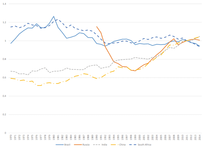
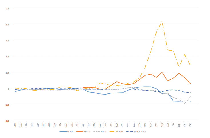
In this section, we apply the Glick-Rogoff model to the fast-growing emerging economies, namely the BRICS countries, Brazil, China, India, Russia, and South Africa. The key determinants of current account change in the Glick-Rogoff model are global and country-specific productivity shocks. To account for the severe negative shocks experienced during the global financial crisis, we estimate the model in two sample periods; one ending in 2008 and the other ending in 2017. In the second subsection, we also apply the extended model with additional macroeconomic variables after we obtain the base results from the original Glick-Rogoff model. In next section, we apply the same model to developed countries, namely Canada, France, Germany, Italy, Japan, the UK, and the USA. We discuss similarities and differences in current account determinants between the BRICS and G7 countries.

Estimation Results of the Basic Glick–Rogoff Model

Global productivity is constructed from the weighted average of the productivities of the G7 countries, namely Canada, France, Germany, Italy, Japan, the UK, and the USA. Alternatively, the first principal component of the productivities of the G7 countries is also used as a measure of global productivity. ${ }^5$ The regression model of Eq. (10) is restated here.
$$
\Delta C A_t=\gamma_1 I_{t-1}+\gamma_2 \Delta A_t^c+\gamma_3 \Delta A_t^W+\varepsilon_t,
$$
From the Glick-Rogoff model, the expected sign of the past investment is positive, that of the first difference of each country’s productivity is negative, and that of the first difference of worldwide productivity is zero; that is, $\gamma_1>0, \gamma_2<0$, and $\gamma_3=$ 0 . The dynamic optimization model of Glick and Rogoff (1995) integrates the endogenous decisions of producers and consumers; therefore, the derived parameters of the model are affected by several sources. However, if we simply decompose the dependent variable, which is the first difference of the current account in terms of private saving and investment, and leave aside the government role, we can observe (in the first equality) the first-degree importance of the current investment and the past investment on the dependent variable. Adjusted for marginal production with respect to investment and capital stock, i.e., $\alpha_I$ and $\alpha_K$, and the impact of past investment shock on the current investment, i.e., $\beta_1$, the coefficient of unity in the equation remains positive, $\gamma_1$, as shown in Eq. (8).
$$
\Delta C A_t \equiv C A_t-C A_{t-1}=\left(S_t-I_t\right)-\left(S_{t-1}-I_{t-1}\right)=\Delta S_t-\Delta I_t
$$
It is also clear that a change in a country’s productivity negatively affects a change in its current account, $\gamma_2$, via a change in investment through the second equality.

经济代写|计量经济学代写Econometrics代考|Extended Models with Other Macroeconomic Variables

Not all empirical models of current account movements emphasize productivity shocks. The advantage of the Glick-Rogoff regression model is its concrete derivation based on the theoretical dynamic model. However, many researchers have continued to explore the possibility of many other macroeconomic variables to explain current account movements, frequently without theoretical models.

Chinn and Prasad (2003) investigated the medium-term determinants of current accounts for a large sample of developed and developing countries. They find that current account balance is positively correlated with government budget balance and the initial level of net foreign assets. Among developing countries, financial deepening is positively associated with current account balance, while trade openness is negatively correlated with current account balance.

Cudre and Hoffmann (2017) and Romelli et al. (2018) also showed that trade openness is a significant driver of current accounts. Romelli et al. (2018) investigated the impact of trade openness on the relationship between the current account and the real exchange rate. They find that during the balance of payment distress episodes, currency depreciations are associated with larger improvements in the current accounts of countries that are more open to trade, and the magnitude of exchange rate depreciations over the adjustment process of current accounts is related to the degree of openness to trade. Cudre and Hoffmann (2017) also find that trade openness is an important factor even across regions within a nation.

Following the recent development of the empirical current account literature, we extended the Glick-Rogoff model with five macroeconomic variables: financial deepening, old dependency ratio, young dependency ratio, net foreign assets, and trade openness. ${ }^8$ First, the fitness of regression substantially improved for Brazil, India, and China. In the shorter sample between 1983 and 2008, the adjusted Rsquared increased from 0.29 to 0.60 for Brazil, from 0.60 to 0.69 for India, and from 0.58 to 0.68 for China. In the longer sample that included the post-crisis period, the adjusted R-squared values were 0.31 for Russia, 0.21 for Brazil, and 0.24 for China; all of these values increased from zero or even negative values of the adjusted R-squared in the basic model estimations.

计量经济学代考

经济代写|计量经济学代写Econometrics代考|Domestic and Global Productivity

在本节中，我们将Glick-Rogoff模型应用于快速增长的新兴经济体，即金砖国家、巴西、中国、印度、俄罗斯和南非。在格利克-罗格夫模型中，决定经常账户变化的关键因素是全球和特定国家的生产率冲击。为了考虑全球金融危机期间经历的严重负面冲击，我们在两个样本期间估计模型;一个是2008年，另一个是2017年。在第二小节中，在获得原始Glick-Rogoff模型的基本结果后，我们还应用了带有额外宏观经济变量的扩展模型。在下一节中，我们将把相同的模型应用于发达国家，即加拿大、法国、德国、意大利、日本、英国和美国。我们讨论了金砖国家和七国集团国家经常账户决定因素的异同。

Glick-Rogoff基本模型的估计结果

全球生产率是由七国集团(G7)(加拿大、法国、德国、意大利、日本、英国和美国)的生产率加权平均值构建而成的。另外，G7国家生产率的第一个主要组成部分也被用作衡量全球生产率的指标。${ }^5$这里重述Eq.(10)的回归模型。
$$
\Delta C A_t=\gamma_1 I_{t-1}+\gamma_2 \Delta A_t^c+\gamma_3 \Delta A_t^W+\varepsilon_t,
$$
从Glick-Rogoff模型看，过去投资的预期符号为正，各国生产率第一次差异的预期符号为负，全球生产率第一次差异的预期符号为零;即$\gamma_1>0, \gamma_2<0$和$\gamma_3=$ 0。Glick和Rogoff(1995)的动态优化模型整合了生产者和消费者的内生决策;因此，模型的导出参数受到多个源的影响。然而，如果我们简单地分解因变量，即经常账户在私人储蓄和投资方面的第一个差异，而不考虑政府的作用，我们可以观察到(在第一个等式中)当前投资和过去投资对因变量的一级重要性。调整了边际产量对投资和资本存量的影响，即$\alpha_I$和$\alpha_K$，以及过去投资冲击对当前投资的影响，即$\beta_1$，方程的统一系数仍然为正，即$\gamma_1$，如式(8)所示。
$$
\Delta C A_t \equiv C A_t-C A_{t-1}=\left(S_t-I_t\right)-\left(S_{t-1}-I_{t-1}\right)=\Delta S_t-\Delta I_t
$$
同样明显的是，一国生产率的变化会通过第二项平等导致投资的变化，从而对其经常账户($\gamma_2$)的变化产生负面影响。

经济代写|计量经济学代写Econometrics代考|Extended Models with Other Macroeconomic Variables

并非所有经常账户变动的实证模型都强调生产率冲击。Glick-Rogoff回归模型的优势在于它在理论动态模型的基础上进行了具体的推导。然而，许多研究人员继续探索许多其他宏观经济变量来解释经常账户变动的可能性，往往没有理论模型。

Chinn和Prasad(2003)调查了大量发达国家和发展中国家经常账户的中期决定因素。他们发现经常项目余额与政府预算余额和初始净外国资产水平呈正相关。在发展中国家，金融深化与经常账户余额正相关，而贸易开放与经常账户余额负相关。

Cudre和Hoffmann(2017)以及Romelli等人(2018)也表明，贸易开放是经常账户的重要驱动因素。Romelli等人(2018)研究了贸易开放对经常账户与实际汇率关系的影响。他们发现，在国际收支困难时期，货币贬值与对贸易更开放的国家经常账户的较大改善有关，而汇率贬值在经常账户调整过程中的幅度与对贸易的开放程度有关。Cudre和Hoffmann(2017)还发现，即使在一个国家的各个地区，贸易开放程度也是一个重要因素。

根据实证经常账户文献的最新发展，我们将Glick-Rogoff模型扩展为五个宏观经济变量:金融深化、老年抚养比、年轻抚养比、净外国资产和贸易开放度。${}^8$首先，巴西、印度和中国的回归适应度显著提高。在1983年至2008年的较短样本中，巴西调整后的Rsquared从0.29增加到0.60，印度从0.60增加到0.69，中国从0.58增加到0.68。在包括危机后时期在内的较长样本中，俄罗斯、巴西和中国的调整后r平方值分别为0.31、0.21和0.24;这些值都是从基本模型估计中调整后的r平方的零甚至负值开始增加的。

经济代写|计量经济学代写Econometrics代考请认准statistics-lab™

统计代写请认准statistics-lab™. statistics-lab™为您的留学生涯保驾护航。

R语言代写	问卷设计与分析代写
PYTHON代写	回归分析与线性模型代写
MATLAB代写	方差分析与试验设计代写
STATA代写	机器学习/统计学习代写
SPSS代写	计量经济学代写
EVIEWS代写	时间序列分析代写
EXCEL代写	深度学习代写
SQL代写	各种数据建模与可视化代写

经济代写|计量经济学代写Econometrics代考|Autoregressive Conditional Betas

Posted on 2023年7月12日2023年7月12日 by statistics-lab

经济代写|计量经济学代写Econometrics代考|Autoregressive Conditional Betas

An alternative to the state space model presented above that also allows a direct specification of dynamic conditional betas has recently been proposed by Darolles et al. (2018). Their model, called CHAR, is a multivariate GARCH model based on the Cholesky decomposition of the $m \times m$ (with $m=N+1$ ) conditional covariance matrix $\Sigma_t$ of $\left(\mathbf{x}_t, y_t\right)^{\prime}$.

As Pourahmadi (1999), let us consider the Cholesky decomposition of $\Sigma_t$, i.e.,
$$
\boldsymbol{\Sigma}t=\boldsymbol{L}_t \boldsymbol{G}_t \boldsymbol{L}_t^{\prime}, $$ where $\boldsymbol{G}_t=\operatorname{diag}\left(g{11, t}, \ldots, g_{m m, t}\right)$ and $\boldsymbol{L}t$ is a lower unitriangular matrix (i.e., triangular with 1 ‘s on the diagonal and 0 ‘s above the diagonal) with element $\ell{i j, t}$ at the row $i$ and column $j$ for $i>j$.

Let us now illustrate this decomposition for $m=3$.
$$
\boldsymbol{L}=\left[\begin{array}{ccc}
1 & 0 & 0 \
l_{21, t} & 1 & 0 \
l_{31, t} & l_{32, t} & 1
\end{array}\right] \quad \boldsymbol{G}=\left[\begin{array}{ccc}
g_{11, t} & 0 & 0 \
0 & g_{22, t} & 0 \
0 & 0 & g_{33, t}
\end{array}\right]
$$
and
$$
\boldsymbol{\Sigma}=\left[\begin{array}{ccc}
g_{11, t} & l_{21, t} g_{11, t} & l_{31, t} g_{11, t} \
l_{21, t} g_{11, t} & l_{21, t}^2 g_{11, t}+g_{22, t} & l_{21, t} l_{31, t} g_{11, t}+l_{32, t} g_{22, t} \
l_{31, t} g_{11, t} & l_{21, t} h_{31, t} g_{11, t}+l_{32, t} g_{22, t} & l_{31, t}^2 g_{11, t}+l_{32, t}^2 g_{22, t}+g_{33, t}
\end{array}\right] .
$$
Darolles et al. (2018) show that if $\boldsymbol{w}t \equiv\left(\mathbf{x}_t, y_t\right)^{\prime}$ has mean $\mathbf{0}$, $$ \begin{aligned} w{i, t} & =\sum_{j=1}^{i-1} \ell_{i j, t} \varepsilon_{j, t}+\varepsilon_{i, t}=\sum_{j=1}^{i-1} \ell_{i j, t}\left(w_{j, t}-\sum_{k=1}^{j-1} \ell_{j k, t} v_{k, t}\right)+\varepsilon_{i, t} \
& =\sum_{j=1}^{i-1} \beta_{i j, t} w_{j, t}+\varepsilon_{i, t} .
\end{aligned}
$$
Interestingly, for $i=m$, the $m$ th equation of the CHAR model is
$$
y_t=\sum_{j=1}^{m-1} \beta_{i j, t} x_{j, t}+\varepsilon_{i, t}
$$
which corresponds to Eq. (35) when $\alpha_t=0, N=m-1$ and $\varepsilon_t=\varepsilon_{i, t}$.

经济代写|计量经济学代写Econometrics代考|Empirical Application on REITs

Real Estate Investment Trusts ${ }^{23}$ (REITs), which are publicly traded real estate companies that own and manage commercial or residential real estate, are attractive alternatives to the mainstream investment choice (e.g., stocks and bonds) since they allow investors to easily access real estate investments without directly owning or managing the underlying assets. ${ }^{24}$ Moreover, the literature on real estate has shown that the inclusion of REITs within one’s portfolio improves the risk-return profile of the portfolio. Compared to other asset classes such as bonds and stocks, they have the characteristics of offering more stable returns and a lower volatility historically. For the purpose of portfolio diversification, it is important to know how the level of exposure of REITs to both the bond market risk and to the stock market risk varies over time. The aim of this section is thus to perform a comparative analysis of the three most advanced modeling techniques (state space, DCB, and ACB) used in estimating the sensitivity of REIT indices to changes in both the bond market and the stock market. Van Nieuwerburgh (2019) argues that a model with a bond market and stock market factor is both the most basic and most natural model of risk for REITs as the bond market beta measures how sensitive REITs are to changes in interest rates and the stock market beta measures how sensitive REITs are to changes in economic activity. ${ }^{25}$ A similar model is used by Allen et al. (2000). Moreover, we note that the addition of three Fama-French risk factors (size, value, and momentum) to the original two-factor model in the study of Van Nieuwerburgh (2019) leaves the bond and stock market betas almost unchanged. As a consequence, we follow Van Nieuwerburgh (2019) and choose to perform our analysis on the following parsimonious two-factor model:
$$
\tilde{r}{\mathrm{REIT}, t}=\alpha_t+\beta{B, t} \tilde{r}{B, t}+\beta{M, t} \widetilde{r}{M, t}+\varepsilon_t, $$ where $\widetilde{r}{\text {REIT }}$ is the excess return on the REIT market, measured by the daily excess return on the FTSE EPRA Nareit index, $\widetilde{r}B$ is the excess return on the bond market, measured by the daily excess return on the sovereign bond index and $\widetilde{r}_M$ is the excess return on the stock market, measured by the daily excess return on the stock market index. Equation (66) corresponds to the conditional risk factor model that we use to estimate conditional betas on day $t$ from a regression of the daily excess REIT index returns on the excess stock market and bond market returns. In the special case where $\boldsymbol{\beta}_t=\left(\beta{B, t}, \beta_{M, t}\right)^{\prime}=\boldsymbol{\beta}$, the betas are restricted to be constant. Note also that for some models, the alpha is allowed to be time-varying as well. However, empirical results (not reported here to save space) suggest that $\alpha_t=\alpha(\forall t)$ once allowing the conditional betas of this two-factor model to be time-varying.

计量经济学代考

经济代写|计量经济学代写Econometrics代考|Autoregressive Conditional Betas

Darolles等人(2018)最近提出了上述状态空间模型的替代方案，该模型也允许直接规范动态条件beta。他们的模型称为CHAR，是一个基于$\left(\mathbf{x}_t, y_t\right)^{\prime}$的$m \times m$(与$m=N+1$)条件协方差矩阵$\Sigma_t$的Cholesky分解的多元GARCH模型。

正如Pourahmadi(1999)，让我们考虑$\Sigma_t$的Cholesky分解，即:
$$
\boldsymbol{\Sigma}t=\boldsymbol{L}t \boldsymbol{G}_t \boldsymbol{L}_t^{\prime}, $$，其中$\boldsymbol{G}_t=\operatorname{diag}\left(g{11, t}, \ldots, g{m m, t}\right)$和$\boldsymbol{L}t$是一个较低的单角矩阵(即三角形，对角线上有1，对角线上有0)，元素$\ell{i j, t}$位于行$i$，列$j$为$i>j$。

现在我们来说明$m=3$的分解。
$$
\boldsymbol{L}=\left[\begin{array}{ccc}
1 & 0 & 0 \
l_{21, t} & 1 & 0 \
l_{31, t} & l_{32, t} & 1
\end{array}\right] \quad \boldsymbol{G}=\left[\begin{array}{ccc}
g_{11, t} & 0 & 0 \
0 & g_{22, t} & 0 \
0 & 0 & g_{33, t}
\end{array}\right]
$$
和
$$
\boldsymbol{\Sigma}=\left[\begin{array}{ccc}
g_{11, t} & l_{21, t} g_{11, t} & l_{31, t} g_{11, t} \
l_{21, t} g_{11, t} & l_{21, t}^2 g_{11, t}+g_{22, t} & l_{21, t} l_{31, t} g_{11, t}+l_{32, t} g_{22, t} \
l_{31, t} g_{11, t} & l_{21, t} h_{31, t} g_{11, t}+l_{32, t} g_{22, t} & l_{31, t}^2 g_{11, t}+l_{32, t}^2 g_{22, t}+g_{33, t}
\end{array}\right] .
$$
Darolles et al.(2018)表明，如果$\boldsymbol{w}t \equiv\left(\mathbf{x}t, y_t\right)^{\prime}$有平均$\mathbf{0}$, $$ \begin{aligned} w{i, t} & =\sum{j=1}^{i-1} \ell_{i j, t} \varepsilon_{j, t}+\varepsilon_{i, t}=\sum_{j=1}^{i-1} \ell_{i j, t}\left(w_{j, t}-\sum_{k=1}^{j-1} \ell_{j k, t} v_{k, t}\right)+\varepsilon_{i, t} \
& =\sum_{j=1}^{i-1} \beta_{i j, t} w_{j, t}+\varepsilon_{i, t} .
\end{aligned}
$$
有趣的是，对于$i=m$, CHAR模型的$m$第1方程为
$$
y_t=\sum_{j=1}^{m-1} \beta_{i j, t} x_{j, t}+\varepsilon_{i, t}
$$
当$\alpha_t=0, N=m-1$和$\varepsilon_t=\varepsilon_{i, t}$时对应式(35)。

经济代写|计量经济学代写Econometrics代考|Empirical Application on REITs

房地产投资信托${ }^{23}$ (REITs)是拥有和管理商业或住宅房地产的上市房地产公司，是主流投资选择(例如股票和债券)的有吸引力的替代品，因为它们允许投资者轻松获得房地产投资，而无需直接拥有或管理相关资产。${ }^{24}$此外，有关房地产的文献表明，在投资组合中纳入REITs可以改善投资组合的风险收益状况。与债券和股票等其他资产类别相比，它们具有更稳定的回报和更低的历史波动性的特点。为了使投资组合多样化，了解房地产投资信托基金对债券市场风险和股票市场风险的敞口水平如何随时间变化是很重要的。因此，本节的目的是对用于估计REIT指数对债券市场和股票市场变化的敏感性的三种最先进的建模技术(状态空间，DCB和ACB)进行比较分析。Van Nieuwerburgh(2019)认为，具有债券市场和股票市场因素的模型是REITs最基本和最自然的风险模型，因为债券市场beta衡量REITs对利率变化的敏感程度，股票市场beta衡量REITs对经济活动变化的敏感程度。${ }^{25}$ Allen等人(2000)使用了一个类似的模型。此外，我们注意到，在Van Nieuwerburgh(2019)的研究中，将三个Fama-French风险因素(规模、价值和动量)添加到原始的双因素模型中，债券和股票市场的贝塔系数几乎没有变化。因此，我们遵循Van Nieuwerburgh(2019)，选择对以下简约的双因素模型进行分析:
$$
\tilde{r}{\mathrm{REIT}, t}=\alpha_t+\beta{B, t} \tilde{r}{B, t}+\beta{M, t} \widetilde{r}{M, t}+\varepsilon_t, $$其中$\widetilde{r}{\text {REIT }}$为房地产投资信托基金市场的超额收益，以富时EPRA Nareit指数的每日超额收益衡量;$\widetilde{r}B$为债券市场的超额收益，以主权债券指数的每日超额收益衡量;$\widetilde{r}M$为股票市场的超额收益，以股票市场指数的每日超额收益衡量。式(66)对应于条件风险因子模型，我们使用该模型从超额股票市场和债券市场回报的每日超额REIT指数回报的回归中估计day $t$的条件贝塔。在$\boldsymbol{\beta}_t=\left(\beta{B, t}, \beta{M, t}\right)^{\prime}=\boldsymbol{\beta}$的特殊情况下，beta被限制为常数。还要注意，对于某些模型，alpha也允许时变。然而，实证结果(为了节省篇幅，这里没有报道)表明$\alpha_t=\alpha(\forall t)$一旦允许这个双因素模型的条件贝塔是时变的。

统计代写请认准statistics-lab™. statistics-lab™为您的留学生涯保驾护航。

R语言代写	问卷设计与分析代写
PYTHON代写	回归分析与线性模型代写
MATLAB代写	方差分析与试验设计代写
STATA代写	机器学习/统计学习代写
SPSS代写	计量经济学代写
EVIEWS代写	时间序列分析代写
EXCEL代写	深度学习代写
SQL代写	各种数据建模与可视化代写

经济代写|计量经济学代写Econometrics代考|Futures Prices and Hedging Demand

Posted on 2023年7月12日2023年7月12日 by statistics-lab

经济代写|计量经济学代写Econometrics代考|Futures Prices and Hedging Demand

Most studies relating CIT trade positions to commodity prices presume that CIT (demand side) initiate the trades and Granger causes the futures price rises. However, CIT positions also reflect producers’ hedging needs (supply side). We need here an identification strategy designed to identify a CIT demand shock in view to assess the genuine contribution of CIT investors to the price evolution. Cheng et al. (2015) used fluctuations in the VIX to isolate trades initiated by CITs and found a positive correlation between CIT position changes and futures prices. Henderson et al. (2015) used commodity-linked note (CLN) issuances to similarly identify trade initiated by financial traders. They found that financial traders “have significantly positive and economically meaningful impacts on commodity futures prices around the pricing dates of the CLNs when the hedge trades are executed and significantly negative price impacts around the determination dates when the hedge trades are unwounded.”
4.4.2 Spot Prices and Macro-Driven Boom
If large inflows of institutional investors on commodity markets can affect the commodity futures prices, the reverse is also true. Indeed, rising commodity prices also attract institutional investors. Most papers based on correlation measures are subject to this endogeneity concern.

Tang and Xiong (2012) studied the correlation of non-energy commodity returns with oil returns and propose a solution. They analyze separately the commodities included in the S\&P GSCI and DJ-UBSCI (treatment group) and the commodities excluded from these indices (control group). They found that the commodities of the treatment group, which are presumed to be subject to commodity index traders’ purchases, had a rise in their correlation with oil returns significantly larger than the one of the commodities in the control group.

As an alternative, Kilian and Murphy (2014) deal with reverse causality by relying on structural VAR modelling and sign restrictions as identification strategy. They use monthly “the percent change in global oil production, a measure of cyclical variation in global real activity, the real price of crude oil, and the change in above-ground global crude oil inventories. The model is identified based on a combination of sign restrictions and bounds on the short-run price elasticities of oil demand and oil supply.”

经济代写|计量经济学代写Econometrics代考|De-Financialization

Weekly futures open interest as reported in CFTC’s CoT fell by $50 \%$ in 2008 but has then recovered and is currently far above its pre-crisis levels. However, all indicators do not support the belief of a constantly rising financialization. The BIS notional value of outstanding OTC commodity derivatives has collapsed from USD 14.1 trillion in 2008 to USD 2.1 trillion in 2019, now stable for more than five years. In addition, the composition of the open interest (in terms of producer, swap dealer, money managers, pother reportable) has remained remarkably stable since 2006 (see Fig. 9 in Bhardwaj et al. 2015).

Further, the presumed effects on financialization on inter-commodity correlation and equity-commodity correlations have vanished as documented via simple rolling correlations in Bhardwaj et al. (2015) and via the explanatory power of multifactor models in Christoffersen et al. (2019). Zhang et al. (2017) explicitly raise the question of “de-financialization,” measured as correlation between equity market and oil and gas markets. Based on a variance-threshold dynamic correlation model, they conclude that financialization persists since 2008.

Discussion
The literature on financialization of commodity markets is challenged by the difficulty to identify the exogenous contribution of financial investors to commodity prices. A clear rise of correlation among commodity prices and between commodity and equity prices has been documented by many from 2004 to around 2010, but only few papers were explicitly accounting for reverse causality (rising prices attract investors) or for hedging supply-demand determination (do financial investors go long because commodity hedgers are on the rise). Those that develop original identification strategy (Tang and Xiong (2012), Cheng et al. (2015), Henderson et al. (2015) among others) show that the debate on the persistent effects of financialization ten years after the financial crisis remains open.

经济代写|计量经济学代写Econometrics代考|How to Measure the Real Exchange Rate

计量经济学代考

经济代写|计量经济学代写Econometrics代考|Futures Prices and Hedging Demand

大多数关于CIT交易头寸与商品价格关系的研究都假设CIT(需求方)发起交易，格兰杰导致期货价格上涨。然而，CIT头寸也反映了生产商的对冲需求(供应方)。在这里，我们需要一个识别策略，旨在识别CIT需求冲击，以评估CIT投资者对价格演变的真正贡献。Cheng et al.(2015)利用VIX波动分离CIT发起的交易，发现CIT持仓变化与期货价格呈正相关。Henderson等人(2015)使用商品关联票据(CLN)发行来识别金融交易员发起的交易。他们发现，金融交易员“在对冲交易执行时，对cln定价日期前后的商品期货价格有显著的积极和经济意义上的影响，而在对冲交易未受损害的确定日期前后，对价格有显著的负面影响。”
4.4.2现货价格与宏观经济繁荣
如果说机构投资者大量流入大宗商品市场会影响大宗商品期货价格，那么反过来也是如此。事实上，不断上涨的大宗商品价格也吸引了机构投资者。大多数基于相关度量的论文都受到这种内生性的关注。

Tang and Xiong(2012)研究了非能源商品收益与石油收益的相关性，并提出了解决方案。他们分别分析了纳入S\&P GSCI和DJ-UBSCI的商品(治疗组)和未纳入这些指数的商品(对照组)。他们发现，假设受商品指数交易员购买影响的实验组的商品，其与石油收益的相关性上升幅度明显大于对照组的商品。

作为替代方案，Kilian和Murphy(2014)通过依赖结构性VAR模型和符号限制作为识别策略来处理反向因果关系。他们使用全球石油产量的月度变化百分比，这是衡量全球实际活动、原油实际价格和全球原油库存变化的周期性变化的指标。该模型是基于石油需求和石油供应的短期价格弹性的符号限制和界限的组合来确定的。”

经济代写|计量经济学代写Econometrics代考|De-Financialization

CFTC的CoT报告的每周期货未平仓合约在2008年下跌了50%，但随后有所回升，目前远高于危机前的水平。然而，并非所有指标都支持金融化持续上升的观点。国际清算银行未结算场外商品衍生品的名义价值已从2008年的14.1万亿美元暴跌至2019年的2.1万亿美元，目前已稳定五年多。此外，自2006年以来，未平仓合约的构成(就生产商、掉期交易商、资金经理、其他可报告方而言)保持了非常稳定(见Bhardwaj et al. 2015的图9)。

此外，Bhardwaj等人(2015)和Christoffersen等人(2019)通过简单滚动相关性和多因素模型的解释力证明，金融化对商品间相关性和股票-商品相关性的假设影响已经消失。Zhang等人(2017)明确提出了“去金融化”的问题，以股票市场与石油和天然气市场之间的相关性来衡量。基于方差-阈值动态相关模型，他们得出结论，金融化自2008年以来持续存在。

讨论
关于商品市场金融化的文献受到难以确定金融投资者对商品价格的外生贡献的挑战。从2004年到2010年左右，大宗商品价格之间以及大宗商品和股票价格之间的相关性明显上升，但只有少数论文明确说明了反向因果关系(价格上涨吸引投资者)或对冲供需决定(金融投资者是否因为大宗商品对冲者的数量上升而做多)。那些制定原始识别策略的人(Tang and Xiong (2012)， Cheng et al. (2015)， Henderson et al.(2015)等)表明，关于金融危机十年后金融化的持续影响的争论仍然存在。

统计代写请认准statistics-lab™. statistics-lab™为您的留学生涯保驾护航。

R语言代写	问卷设计与分析代写
PYTHON代写	回归分析与线性模型代写
MATLAB代写	方差分析与试验设计代写
STATA代写	机器学习/统计学习代写
SPSS代写	计量经济学代写
EVIEWS代写	时间序列分析代写
EXCEL代写	深度学习代写
SQL代写	各种数据建模与可视化代写

经济代写|计量经济学代写Econometrics代考|How to Measure the Real Exchange Rate

Posted on 2023年6月20日2023年6月20日 by statistics-lab

经济代写|计量经济学代写Econometrics代考|How to Measure the Real Exchange Rate

Similar to nominal exchange rates, real exchange rates can be computed on a bilateral or on an effective basis.

In their seminal contribution, Chen and Rogoff (2003) studied commodity currencies with exchange rates expressed in USD. One obvious limit of bilateral exchange rates is that it does not isolate from factors that are specific to the reference currency area, namely the dollar zone. Checking the robustness of the results on alternative currencies is a necessity when working with bilateral exchange rates. Chen and Rogoff therefore compared their results with those obtained with exchange rates expressed in GBP.

Most studies on commodity currencies (Cashin et al. 2004; Bodart et al. 2012, 2015; Coudert et al. 2011) rely on the effective version of the exchange rate, defined as trade-weighted multilateral real exchange rate, where the weights are specific to each country trade network, as set out in Eq. (7)
$$
\mathrm{RER}{i t}=\sum{j=1}^J w_{i j} \mathrm{RER}{i j t} $$ where $\mathrm{RER}{i t}$ is the real effective exchange rate of country $i, \operatorname{RER}{i j t}$ is the real bilateral exchange of country $i$ with country $j$, where $w{i j}$ is the weight associated to $\mathrm{RER}_{i j t}$, and where $J$ is the number of countries considered in the real effective exchange rate formula of country $i$. Such series are available from IMF-IFS database, or alternatively from Darvas (2012).

The strength of effective rates is that real exchange rates are measured in terms of a basket of currencies, thereby diluting the fluctuations due to country $j$ shocks. The weakness is that the basket is country specific, that is, $w_{i j}$ depends on $i$. Using countryspecific trade weights is mainly justified for studies focusing on competitiveness. An alternative is to use a fixed basket of currencies (in the vein of special drawing rights or of the Libra), set identically for all investigated countries, that is, $w_{i j}=w_j$ in Eq. (7). Chen and Rogoff (2003) took this option by replicating their analysis on Canada, Australia, and New Zealand by looking at the exchange rate with the socalled broad index, a composite of over 30 non-US-dollar currencies. Surprisingly, this interesting practice has not been much followed.

经济代写|计量经济学代写Econometrics代考|Real Versus Nominal

As discussed by Chinn (2006), we often face a trade-off between using the most appropriate real exchange rate measure conceptually, and the most readily available data.

In practice, one only has a choice of a few price deflators. At the monthly frequency, they include the consumer price index (CPI), producer price index (PPI), wholesale price index (WPI), and export price index. At lower frequencies, such as quarterly, the set of deflators increases somewhat, to include the GDP deflator, unit labor costs, and price indices for the components of GDP, such as the personal consumption expenditure (PCE) deflator.

Typically, the CPI is thought of as weighting fairly heavily non-traded goods such as consumer services. Similarly, the GDP deflator and the CPI weigh expenditures on non-tradables in proportion to their importance in the aggregate economy. In contrast, the PPI and WPI exclude retail sales services that are likely to be non-traded.

Due to availability constraints for long periods and the need of a large enough set of developing countries, most studies use CPI-real exchange rates (Chen and Rogoff 2003; Cashin et al. 2004; Bodart et al. 2012, 2015), as provided by the IMF-IFS database for a wide set of countries and years.

Clearly, for purposes of calculating the relative price of goods and services that are tradable, the preferred measure would have been the exchange rate deflated by PPIs or WPIs were the data available. It is worth noting that a recent empirical paper of Ahn, Mano, and Zhou (2017), compared CPI, GDP, and ULC deflators in the context of the expenditure switching mechanism studies. It supports Chinn (2006) statement that the choice of the deflator may have considerable effects on the empirical conclusions.

计量经济学代考

经济代写|计量经济学代写Econometrics代考|How to Measure the Real Exchange Rate

与名义汇率类似，实际汇率可以在双边或有效基础上计算。

Chen和Rogoff(2003)在其开创性贡献中研究了以美元表示汇率的商品货币。双边汇率的一个明显限制是，它没有与参考货币区(即美元区)特有的因素隔离开来。在处理双边汇率时，检查替代货币结果的稳健性是必要的。因此，Chen和Rogoff将他们的结果与以英镑表示的汇率得到的结果进行了比较。

大多数关于商品货币的研究(Cashin et al. 2004;Bodart et al. 2012, 2015;Coudert et al. 2011)依赖于汇率的有效版本，定义为贸易加权多边实际汇率，其中权重特定于每个国家的贸易网络，如式(7)所示。
$$
\mathrm{RER}{i t}=\sum{j=1}^J w_{i j} \mathrm{RER}{i j t} $$ 在哪里 $\mathrm{RER}{i t}$ 一国的实际有效汇率是多少 $i, \operatorname{RER}{i j t}$ 真正的双边交流是国家的吗 $i$ 有国家 $j$，其中 $w{i j}$ 重量与 $\mathrm{RER}_{i j t}$，在哪里? $J$ 国家的实际有效汇率公式中是否考虑了国家的数量 $i$．这些序列可从IMF-IFS数据库获得，也可从Darvas(2012)获得。

有效汇率的优势在于，实际汇率是以一篮子货币来衡量的，从而冲淡了国家$j$冲击造成的波动。缺点在于篮子是针对特定国家的，也就是说，$w_{i j}$取决于$i$。使用国别贸易权重主要是为了研究竞争力。另一种选择是使用固定的一篮子货币(以特别提款权或Libra的形式)，为所有被调查的国家设置相同的货币，即公式(7)中的$w_{i j}=w_j$。Chen和Rogoff(2003)通过使用所谓的广义指数(由30多种非美元货币组成的综合指数)观察汇率，复制了他们对加拿大、澳大利亚和新西兰的分析，采用了这一选择。令人惊讶的是，这种有趣的做法并没有得到多少效仿。

经济代写|计量经济学代写Econometrics代考|Real Versus Nominal

正如Chinn(2006)所讨论的，在概念上使用最合适的实际汇率度量和最容易获得的数据之间，我们经常面临权衡。

实际上，人们只能选择几种价格平减指数。按月频率，它们包括消费者价格指数(CPI)、生产者价格指数(PPI)、批发价格指数(WPI)和出口价格指数。在较低的频率下，如季度，平减指数会有所增加，包括GDP平减指数、单位劳动力成本和GDP组成部分的价格指数，如个人消费支出(PCE)平减指数。

通常，人们认为CPI对非贸易商品(如消费服务)的权重相当大。同样，GDP平减指数和CPI衡量的是非贸易品支出与其在总体经济中的重要性成比例。相比之下，PPI和WPI不包括可能非贸易的零售销售服务。

由于长期的可用性限制和需要足够多的发展中国家，大多数研究使用cpi -实际汇率(Chen和Rogoff 2003;Cashin et al. 2004;Bodart et al. 2012, 2015)，由IMF-IFS数据库提供，适用于广泛的国家和年份。

显然，为了计算可贸易商品和服务的相对价格，首选的衡量标准应该是按购买力平价(ppi)或wpi(如果有数据的话)折算的汇率。值得注意的是，Ahn、Mano和Zhou(2017)最近的一篇实证论文在支出转换机制研究的背景下比较了CPI、GDP和ULC平减指数。它支持了Chinn(2006)关于平减指数的选择可能对实证结论有相当大影响的说法。

统计代写请认准statistics-lab™. statistics-lab™为您的留学生涯保驾护航。

金融工程代写

金融工程是使用数学技术来解决金融问题。金融工程使用计算机科学、统计学、经济学和应用数学领域的工具和知识来解决当前的金融问题，以及设计新的和创新的金融产品。

非参数统计代写

非参数统计指的是一种统计方法，其中不假设数据来自于由少数参数决定的规定模型；这种模型的例子包括正态分布模型和线性回归模型。

广义线性模型代考

广义线性模型（GLM）归属统计学领域，是一种应用灵活的线性回归模型。该模型允许因变量的偏差分布有除了正态分布之外的其它分布。

术语广义线性模型（GLM）通常是指给定连续和/或分类预测因素的连续响应变量的常规线性回归模型。它包括多元线性回归，以及方差分析和方差分析（仅含固定效应）。

有限元方法代写

有限元方法（FEM）是一种流行的方法，用于数值解决工程和数学建模中出现的微分方程。典型的问题领域包括结构分析、传热、流体流动、质量运输和电磁势等传统领域。

有限元是一种通用的数值方法，用于解决两个或三个空间变量的偏微分方程（即一些边界值问题）。为了解决一个问题，有限元将一个大系统细分为更小、更简单的部分，称为有限元。这是通过在空间维度上的特定空间离散化来实现的，它是通过构建对象的网格来实现的：用于求解的数值域，它有有限数量的点。边界值问题的有限元方法表述最终导致一个代数方程组。该方法在域上对未知函数进行逼近。[1] 然后将模拟这些有限元的简单方程组合成一个更大的方程系统，以模拟整个问题。然后，有限元通过变化微积分使相关的误差函数最小化来逼近一个解决方案。

tatistics-lab作为专业的留学生服务机构，多年来已为美国、英国、加拿大、澳洲等留学热门地的学生提供专业的学术服务，包括但不限于Essay代写，Assignment代写，Dissertation代写，Report代写，小组作业代写，Proposal代写，Paper代写，Presentation代写，计算机作业代写，论文修改和润色，网课代做，exam代考等等。写作范围涵盖高中，本科，研究生等海外留学全阶段，辐射金融，经济学，会计学，审计学，管理学等全球99%专业科目。写作团队既有专业英语母语作者，也有海外名校硕博留学生，每位写作老师都拥有过硬的语言能力，专业的学科背景和学术写作经验。我们承诺100%原创，100%专业，100%准时，100%满意。

随机分析代写

随机微积分是数学的一个分支，对随机过程进行操作。它允许为随机过程的积分定义一个关于随机过程的一致的积分理论。这个领域是由日本数学家伊藤清在第二次世界大战期间创建并开始的。

时间序列分析代写

随机过程，是依赖于参数的一组随机变量的全体，参数通常是时间。随机变量是随机现象的数量表现，其时间序列是一组按照时间发生先后顺序进行排列的数据点序列。通常一组时间序列的时间间隔为一恒定值（如1秒，5分钟，12小时，7天，1年），因此时间序列可以作为离散时间数据进行分析处理。研究时间序列数据的意义在于现实中，往往需要研究某个事物其随时间发展变化的规律。这就需要通过研究该事物过去发展的历史记录，以得到其自身发展的规律。

回归分析代写

多元回归分析渐进（Multiple Regression Analysis Asymptotics）属于计量经济学领域，主要是一种数学上的统计分析方法，可以分析复杂情况下各影响因素的数学关系，在自然科学、社会和经济学等多个领域内应用广泛。

MATLAB代写

MATLAB 是一种用于技术计算的高性能语言。它将计算、可视化和编程集成在一个易于使用的环境中，其中问题和解决方案以熟悉的数学符号表示。典型用途包括：数学和计算算法开发建模、仿真和原型制作数据分析、探索和可视化科学和工程图形应用程序开发，包括图形用户界面构建MATLAB 是一个交互式系统，其基本数据元素是一个不需要维度的数组。这使您可以解决许多技术计算问题，尤其是那些具有矩阵和向量公式的问题，而只需用 C 或 Fortran 等标量非交互式语言编写程序所需的时间的一小部分。MATLAB 名称代表矩阵实验室。MATLAB 最初的编写目的是提供对由 LINPACK 和 EISPACK 项目开发的矩阵软件的轻松访问，这两个项目共同代表了矩阵计算软件的最新技术。MATLAB 经过多年的发展，得到了许多用户的投入。在大学环境中，它是数学、工程和科学入门和高级课程的标准教学工具。在工业领域，MATLAB 是高效研究、开发和分析的首选工具。MATLAB 具有一系列称为工具箱的特定于应用程序的解决方案。对于大多数 MATLAB 用户来说非常重要，工具箱允许您学习和应用专业技术。工具箱是 MATLAB 函数（M 文件）的综合集合，可扩展 MATLAB 环境以解决特定类别的问题。可用工具箱的领域包括信号处理、控制系统、神经网络、模糊逻辑、小波、仿真等。

R语言代写	问卷设计与分析代写
PYTHON代写	回归分析与线性模型代写
MATLAB代写	方差分析与试验设计代写
STATA代写	机器学习/统计学习代写
SPSS代写	计量经济学代写
EVIEWS代写	时间序列分析代写
EXCEL代写	深度学习代写
SQL代写	各种数据建模与可视化代写

经济代写|计量经济学代写Econometrics代考|Deterministic Trends

Posted on 2023年6月20日2023年6月20日 by statistics-lab

经济代写|计量经济学代写Econometrics代考|Deterministic Trends

First, let us assume that the relative commodity price series is generated by a trendstationary (TS) data process as follows
$$
\mathrm{COMP}_{\mathrm{t}}=\alpha+\beta t+\varepsilon_t
$$
where $\mathrm{COMP}_t$ is the logarithm of the commodity price indice, where $t$ is an annual deterministic trend, where $\varepsilon_t$ is a stationary process with mean equal to zero, an ARMA for example, and where the sign and significance of $\beta$ lead to conclusions on the PSH. Most studies based on this methodology (Sapsford 1985; Grilli and Yang 1988) found support to the PSH, in other words $\beta$ was found to be significantly negative.

Of course, these conclusions are subject to the validity of the stationarity assumption. Non-stationarity of the error terms could lead to spurious rejection of the null $\beta=0$ and to spurious support of the PSH. Cuddington and Urzua (1989) were the first to carry out unit-root tests on the Grilli-Yang commodity price dataset. Similarly, Kim et al. (2003) showed that the 24 commodity price series contained in the standard Grilli-Yang commodity price index are characterized by unit-root behaviors (18 commodities) or quasi-unit roots ( 6 commodities). Similar results were reported by Cuddington (1992) and Newbold et al. (2005).

经济代写|计量经济学代写Econometrics代考|Stochastic Trends

Consequently, we can assume that the relative commodity price series are generated by a difference-stationary (DS) process as follows
$$
\Delta \mathrm{COMP}_t=\beta+u_t
$$
where $\Delta P_t$ is the differenced logarithm of the commodity price index, where $u_t$ is a stationary process, an ARMA for example, with mean equal to zero, and where the sign and significance of $\beta$ leads to conclusions on the PSH. Kim et al. (2003) accounted for non-stationarity and find much less support to the PSH. Indeed, using the same 24 commodity prices of the Grilli-Yang database, they observe that the null hypothesis of $\beta=0$ is much less frequently rejected with a non-stationary process specification than in stationary models.

The finding that most commodity price series largely behave like random walks is not anodine. A shock to the price of, say, copper today would thus be permanent. Copper price would no longer revert to any stable, long-run values/trends. As a consequence, stabilization mechanism as the one implemented by Chile, whereby asset accumulation is conditioned on copper prices being above a long-term level, would theoretically no longer be sustainable as it relies on the concept of a stable level/trend.

Detection of unit roots remains subject to some caution. It might be spuriously derived from a bad specification of the data-generating process or due to the wellknown lack of power of standard non-stationary tests (Schwert 1987). We now consider extensions related to these two possibilities and see that the conclusions supporting the PSH lose their strength.

计量经济学代考

经济代写|计量经济学代写Econometrics代考|Deterministic Trends

首先，让我们假设相对商品价格序列是由趋势平稳(TS)数据过程生成的，如下所示
$$
\mathrm{COMP}_{\mathrm{t}}=\alpha+\beta t+\varepsilon_t
$$
其中$\mathrm{COMP}_t$是商品价格指数的对数，$t$是年度确定性趋势，$\varepsilon_t$是均值等于零的平稳过程，例如ARMA, $\beta$的符号和显著性得出了关于PSH的结论。大多数研究基于这种方法(Sapsford 1985;Grilli和Yang(1988)发现对PSH的支持，换句话说$\beta$被发现是显着负的。

当然，这些结论取决于平稳性假设的有效性。误差项的非平稳性可能导致对null $\beta=0$的虚假拒绝和对PSH的虚假支持。Cuddington和Urzua(1989)首先对grill – yang商品价格数据集进行了单位根检验。同样，Kim et al.(2003)表明，标准grill – yang商品价格指数中包含的24个商品价格序列具有单位根行为(18种商品)或准单位根行为(6种商品)的特征。Cuddington(1992)和Newbold et al.(2005)也报道了类似的结果。

经济代写|计量经济学代写Econometrics代考|Stochastic Trends

因此，我们可以假设相对商品价格序列是由一个差分平稳(DS)过程产生的
$$
\Delta \mathrm{COMP}_t=\beta+u_t
$$
其中$\Delta P_t$是商品价格指数的差分对数，其中$u_t$是一个平稳过程，例如ARMA，其平均值等于零，其中$\beta$的符号和显著性导致关于PSH的结论。Kim等人(2003)解释了非平稳性，发现对PSH的支持要少得多。事实上，使用grili – yang数据库中相同的24种商品价格，他们观察到，与平稳模型相比，非平稳过程规范中$\beta=0$的零假设被拒绝的频率要低得多。

大多数大宗商品价格序列在很大程度上表现得像随机漫步，这一发现并不是一件好事。因此，对(比如说)铜价的冲击将是永久性的。铜价将不再恢复到任何稳定的长期价值/趋势。因此，智利实施的稳定机制，即资产积累以铜价高于长期水平为条件，理论上将不再可持续，因为它依赖于稳定水平/趋势的概念。

单位根的检测仍然需要一些谨慎。它可能是由于数据生成过程的不良规范或由于众所周知的标准非平稳测试缺乏力量而产生的虚假结果(Schwert 1987)。我们现在考虑与这两种可能性相关的扩展，并看到支持PSH的结论失去了力量。

统计代写请认准statistics-lab™. statistics-lab™为您的留学生涯保驾护航。

金融工程代写

非参数统计代写

非参数统计指的是一种统计方法，其中不假设数据来自于由少数参数决定的规定模型；这种模型的例子包括正态分布模型和线性回归模型。

广义线性模型代考

广义线性模型（GLM）归属统计学领域，是一种应用灵活的线性回归模型。该模型允许因变量的偏差分布有除了正态分布之外的其它分布。

有限元方法代写

随机分析代写

时间序列分析代写

回归分析代写

MATLAB代写

R语言代写	问卷设计与分析代写
PYTHON代写	回归分析与线性模型代写
MATLAB代写	方差分析与试验设计代写
STATA代写	机器学习/统计学习代写
SPSS代写	计量经济学代写
EVIEWS代写	时间序列分析代写
EXCEL代写	深度学习代写
SQL代写	各种数据建模与可视化代写

经济代写|计量经济学代写Econometrics代考|Structural Generalized Impulse-Response Function (SGIRF) Analysis of US Productivity Shocks

Posted on 2023年6月20日2023年6月20日 by statistics-lab

经济代写|计量经济学代写Econometrics代考|Structural Generalized Impulse-Response Function (SGIRF) Analysis of US Productivity Shocks

The identification of shocks has been a major issue in GVAR models. In order to conduct dynamic analysis, the vast majority of research papers using GVAR models rely on the GIRF proposed by Koop et al. (1996) and further developed by Pesaran and Shin (1998). The identification of shocks in a GVAR model is complicated due to the cross-country interactions and high dimensionality of the model.

The identification in a traditional VAR analysis is usually achieved by using the orthogonalized impulse-response functions (OIRFs) that require a certain ordering of variables. This approach is often not suitable for GVAR models, as it requires ordering not only of the variables, but also countries. As a result, when a large number of variables and countries are included in the model, it becomes difficult to justify such ordering based on economic theory and empirical findings. The advantage of GIRFs is that they are invariant to the ordering of countries and variables. This is very convenient for models like GVAR that involve many countries and variables. However, it comes at a cost. Critics often argue that in GIRFs, the error terms are not orthogonal and it allows correlation among them. This, in turn, makes economic interpretation of shocks difficult.

We take this into account by using SGIRFs instead of GIRFs. The SGIRF allows the most dominant economy in the model to be ordered first and also its variables to have certain ordering. Since the main aim of this paper is to investigate spillover effects of productivity shocks arising in the USA, the largest economy in the model, the USA and its variables are ordered first. This means that the identifying scheme for the model of the USA is based on a lower-triangular Cholesky decomposition and has the following ordering: [R\&D, TFP, capital, GDP]’. Thus, for the USA, R\&D is ordered first, followed by TFP because greater expenditure on R\&D could increase TFP. This assumes that R\&D spending affects TFP contemporaneously, but not vice versa. TFP is then followed by capital and GDP. This ordering system assumes that GDP is the most endogenous variable, which is a realistic assumption to make. Other countries and their variables are kept unrestricted. More about the GIRF and SGIRF is discussed in the appendix.

经济代写|计量经济学代写Econometrics代考|Productivity Shocks in the EU, Non-OECD, and Others

Figures 4, 5 and 6 show the response of the same variables to one standard deviation (SD) positive shock in ‘the EU,’ ‘non-OECD,’ and ‘Others’ country groups, respectively. The first row of each figure shows the response of GDP to a TFP shock. The EU’s TFP shock does have some positive and significant effects on GDP of the EU and the other country groups. Compared to the US TFP shock, these reactions are smaller in magnitude. EU’s TFP shock also increases US R\&D and has a further positive effect on its own TFP. Such reactions are, however, significant for a very short period of time. A shock to the non-OECD group’s TFP has some positive significant effect on its own GDP, but spillover effects are not highly significant. A shock to the final group ‘Others’ has no significant effect on the GDP of any country groups either. In terms of the effect on other variables, results are not very significant.

Interestingly, a positive TFP shock is associated with increases in R\&D spending for the USA and other country groups. This might be due to the size of the US R\&D and the fact that US multinational firms are much more global in terms of investing in other country groups. According to the Forbes Global 2000 that lists top 2000 companies in the world, the USA was ranked first in terms of the number of firms included in this list. An increase in productivity in the rest of the world creates greater incentives for them to expand their business by spending more on R\&D. Put it differently, productivity improvements in other country groups are dependent upon productivity advances in the USA. On the contrary, R\&D spending in the EU decreases when there is a positive TFP shock in ‘Non-OECD’ and ‘Others’ country groups. These results might explain why the EU is still lagging behind the USA in terms of research and innovation and are in line with findings of Miller and Atkinson (2014). While the USA is able to make best use of productivity improvements in other countries, the rest of the world fails to do so.

计量经济学代考

经济代写|计量经济学代写Econometrics代考|Structural Generalized Impulse-Response Function (SGIRF) Analysis of US Productivity Shocks

冲击的识别一直是GVAR模型中的一个主要问题。为了进行动态分析，绝大多数使用GVAR模型的研究论文依赖于Koop等人(1996)提出并由Pesaran和Shin(1998)进一步发展的GIRF。由于GVAR模型的跨国相互作用和高维性，使得GVAR模型中冲击的识别非常复杂。

在传统的VAR分析中，识别通常是通过使用正交脉冲响应函数(oirf)来实现的，这需要一定的变量顺序。这种方法通常不适用于GVAR模型，因为它不仅需要对变量进行排序，而且需要对国家进行排序。因此，当模型中包含大量变量和国家时，很难根据经济理论和实证结果证明这种排序是合理的。全球气候变化基金的优势在于，它们对国家和变量的排序是不变的。这对于像GVAR这样涉及许多国家和变量的模型来说是非常方便的。然而，这是有代价的。批评者经常认为，在girf中，误差项不是正交的，它允许它们之间的相关性。这反过来又使得对冲击的经济解释变得困难。

我们通过使用sgirf而不是girf来考虑这一点。SGIRF允许在模型中最具主导地位的经济体被优先排序，并且其变量也具有一定的排序。由于本文的主要目的是研究模型中最大的经济体美国生产率冲击的溢出效应，因此将美国及其变量放在首位。这意味着美国模型的识别方案基于低三角Cholesky分解，并具有以下顺序:[R\&D, TFP，资本，GDP]。因此，对于美国来说，研发是首先订购的，其次是TFP，因为更多的研发支出可以提高TFP。这假设研发支出同时影响TFP，而不是相反。TFP之后是资本和GDP。这个排序系统假设GDP是最内生的变量，这是一个现实的假设。其他国家及其变量不受限制。关于全球环境基金和SGIRF的更多信息将在附录中讨论。

经济代写|计量经济学代写Econometrics代考|Productivity Shocks in the EU, Non-OECD, and Others

图4、图5和图6分别显示了“欧盟”、“非经合组织”和“其他”国家组中相同变量对一个标准差(SD)正冲击的反应。每个数字的第一行显示了GDP对TFP冲击的反应。欧盟的TFP冲击确实对欧盟和其他国家集团的GDP产生了一些积极而显著的影响。与美国的TFP冲击相比，这些反应的规模较小。欧盟的TFP冲击也增加了美国的研发，并对其自身的TFP产生了进一步的积极影响。然而，这种反应在很短的时间内是显著的。对非经合组织成员国TFP的冲击对其国内生产总值有一定的正向显著影响，但溢出效应并不十分显著。对最后一组“其他”的冲击对任何国家组的GDP也没有显著影响。至于对其他变量的影响，结果不是很显著。

有趣的是，对美国和其他国家群体来说，TFP的积极冲击与研发支出的增加有关。这可能是由于美国研发的规模，以及美国跨国公司在投资其他国家集团方面更加全球化的事实。根据福布斯全球2000强公司排名，美国在上榜公司数量上排名第一。世界其他地区生产率的提高为它们提供了更大的动力，促使它们通过加大研发支出来扩大业务。换句话说，其他国家集团的生产率提高取决于美国生产率的提高。相反，当“非经合组织”和“其他”国家群体的TFP受到积极冲击时，欧盟的研发支出就会减少。这些结果可能解释了为什么欧盟在研究和创新方面仍然落后于美国，并且与Miller和Atkinson(2014)的研究结果一致。虽然美国能够最大限度地利用其他国家的生产力提高，但世界其他国家却未能做到这一点。

统计代写请认准statistics-lab™. statistics-lab™为您的留学生涯保驾护航。

金融工程代写

非参数统计代写

非参数统计指的是一种统计方法，其中不假设数据来自于由少数参数决定的规定模型；这种模型的例子包括正态分布模型和线性回归模型。

广义线性模型代考

广义线性模型（GLM）归属统计学领域，是一种应用灵活的线性回归模型。该模型允许因变量的偏差分布有除了正态分布之外的其它分布。

有限元方法代写

随机分析代写

时间序列分析代写

回归分析代写

MATLAB代写

R语言代写	问卷设计与分析代写
PYTHON代写	回归分析与线性模型代写
MATLAB代写	方差分析与试验设计代写
STATA代写	机器学习/统计学习代写
SPSS代写	计量经济学代写
EVIEWS代写	时间序列分析代写
EXCEL代写	深度学习代写
SQL代写	各种数据建模与可视化代写

经济代写|计量经济学代写Econometrics代考|Time-Varying VECM Specification for Wealth Effects

Posted on 2023年6月6日2023年6月6日 by statistics-lab

经济代写|计量经济学代写Econometrics代考|Time-Varying VECM Specification for Wealth Effects

This specification is more original as it enables both the long-run relationship (cointegration relationship) and the ECM to exhibit nonlinearity. ${ }^8$ This novel specification allows a generalization of both first and second specifications and offers a more original econometric framework to investigate complex wealth effects.

Formally, following Bierens and Martins (2010), we first compute the multivariate time-varying cointegration. Bierens et Martins (2010) explained that long-run coefficients of the $\operatorname{VAR}(\mathrm{p})$ are allowed to change with time and can be approximated by a finite sum of Chebyshev polynomials. In this way, the Bierens and Martins methodology considers a multivariate VECM framework for which the Johansen (1991) model is a special case.
Thus we start with the following TV-VECM of order $p$ :
$$
\Delta Z_t=\mu+\alpha \beta_t^{\prime} Z_{t-1}+\sum_{j=1}^{p-1} \Gamma_j \Delta Z_{t-j}+\varepsilon_t, \varepsilon_t \sim \text { i.i.d. } N_k(0, \Omega), t=1, \ldots, T .
$$
With $Z_t=\left(C_t, T W_t\right.$, Income $\left._t\right)$ for the model with aggregate data or $Z_t=$ $\left(C_t, F W_t, H W_t\right.$, Income $\left._t\right)$ when considering the disaggregate data. $\mu, \alpha$ and $\beta$ are $3 \times 1$ fixed coefficients vectors.

Contrary to the standard VECM from Johansen (1991), the coefficients may be time-varying. Assuming that the function of discrete time $\beta_t$ is smooth in line with Bierens and Martins (2010), we thus have the following: $\beta_t=\beta_m\left(\frac{t}{T}\right)=$ $\sum_{i=0}^m \xi_{i, T} P_{i, T}(t)$ where the orthonormal Chebyshev time polynomials $P_{i, T}(t)$ are defined by $P_{0, T}(t)=1, P_{i, T}(t)=\sqrt{2} \cos \left(\frac{i \pi(t-0.5)}{T}\right), t=1,2, \ldots, T, i=$ $1,2, \ldots, m$ and $\xi_{i, T}=\frac{1}{T} \sum_{t=1}^T \beta_t P_{i, T}(t)$ are unknown $k \times r$ matrices with $k$ the number of variables and $r$ the rank.

经济代写|计量经济学代写Econometrics代考|Data and Preliminary Analysis

Data are quarterly and cover the period 1987Q1 to 2011Q4. They concern France and are obtained from financial and non-financial national accounts. Consumption is defined as the household’s total expenditures, while Income corresponds to the flow of human wealth and is measured by disposable income net of property and imputed rents. Financial wealth consists in the household’s financial assets net of debts, whereas Housing wealth consists in tangible assets (land and housing). Our study extended the one by Chauvin and Damette (2011), who used similar data over the period 1987-2008, by focusing on nonlinearity in the wealth-consumption relationship. It also extended their study through the use of more recent data to outline the effect of the subprime crisis on the Consumption/Wealth relationship. More details about the data are reported in Fig. 1.

First, the analysis of Fig. 1-which reports consumption, income, total wealth, HW and $\mathrm{FW}$ in logarithms-shows that series are a priori non-stationary in level. Furthermore, consumption and $\mathrm{HW}$ indicate some smoothness and seem less volatile than income, FW and Total Wealth (TW). We also plot the dynamics of the FW/Income and HW/Income ratios, using the disposable income net of property and imputed rents. These ratios show some French stylized facts associated with the preference of French householders for real estate investments to financial investments. This fact is more marked after the 2000 dotcom bubble.

Second, we tested for the presence of a unit root in the data. To this end, we performed both the usual unit root tests-ADF of Dickey-Fuller (1979) and DFGLS of Elliot, Rothenberg, Stock (1996)_and also a unit root test with structural breaks of Zivot and Andrews (1992) and Kapetanios et al. (2003) in the nonlinear STAR framework. Accordingly, all series are integrated of order one, noted I(1). ${ }^9$ We focused thereafter on the variables in first difference.

计量经济学代考

经济代写|计量经济学代写Econometrics代考|Time-Varying VECM Specification for Wealth Effects

该规范更具原创性，因为它使长期关系(协整关系)和ECM都显示出非线性。${ }^8$这个新颖的规范允许第一和第二规范的概括，并提供了一个更原始的计量经济学框架来研究复杂的财富效应。

形式上，继Bierens和Martins(2010)之后，我们首先计算多元时变协整。Bierens et Martins(2010)解释说，$\operatorname{VAR}(\mathrm{p})$的长期系数允许随时间变化，并且可以用有限的切比雪夫多项式求和来近似。通过这种方式，Bierens和Martins的方法考虑了一个多元VECM框架，其中Johansen(1991)模型是一个特例。
因此，我们从以下顺序为$p$的TV-VECM开始:
$$
\Delta Z_t=\mu+\alpha \beta_t^{\prime} Z_{t-1}+\sum_{j=1}^{p-1} \Gamma_j \Delta Z_{t-j}+\varepsilon_t, \varepsilon_t \sim \text { i.i.d. } N_k(0, \Omega), t=1, \ldots, T .
$$
对于具有聚合数据的模型，使用$Z_t=\left(C_t, T W_t\right.$、Income $\left._t\right)$;对于考虑非聚合数据的模型，使用$Z_t=$$\left(C_t, F W_t, H W_t\right.$、Income $\left._t\right)$。$\mu, \alpha$和$\beta$为$3 \times 1$定系数向量。

与Johansen(1991)的标准VECM相反，系数可能是时变的。假设离散时间函数$\beta_t$与Bierens and Martins(2010)一致是光滑的，我们得到:$\beta_t=\beta_m\left(\frac{t}{T}\right)=$$\sum_{i=0}^m \xi_{i, T} P_{i, T}(t)$其中标准正交Chebyshev时间多项式$P_{i, T}(t)$定义为$P_{0, T}(t)=1, P_{i, T}(t)=\sqrt{2} \cos \left(\frac{i \pi(t-0.5)}{T}\right), t=1,2, \ldots, T, i=$, $1,2, \ldots, m$和$\xi_{i, T}=\frac{1}{T} \sum_{t=1}^T \beta_t P_{i, T}(t)$是未知的$k \times r$矩阵，其中$k$为变量数，$r$为秩。

经济代写|计量经济学代写Econometrics代考|Data and Preliminary Analysis

数据为季度数据，涵盖1987年第一季度至2011年第四季度。它们涉及法国，是从财政和非财政国民核算中获得的。消费被定义为家庭的总支出，而收入则对应于人类财富的流动，用扣除财产和估算租金的可支配收入来衡量。金融财富是指扣除债务后的家庭金融资产，而住房财富是指有形资产(土地和住房)。我们的研究扩展了Chauvin和Damette(2011)的研究，他们使用了1987-2008年期间的类似数据，通过关注财富-消费关系的非线性。它还通过使用最近的数据来扩展他们的研究，以概述次贷危机对消费/财富关系的影响。关于数据的更多细节见图1。

首先，对图1(以对数形式报告了消费、收入、总财富、HW和$\mathrm{FW}$)的分析表明，序列在水平上是先验的非平稳的。此外，消费和$\mathrm{HW}$显示出一些平滑，似乎比收入，FW和总财富(TW)波动更小。我们还利用财产和估算租金的净可支配收入，绘制了FW/Income和HW/Income比率的动态图。这些比率显示了一些法国式的事实，与法国家庭对房地产投资的偏好有关，而不是金融投资。这一事实在2000年互联网泡沫之后更为明显。

其次，我们测试了数据中是否存在单位根。为此，我们在非线性STAR框架下进行了通常的单位根检验——Dickey-Fuller(1979)的adf和Elliot, Rothenberg, Stock(1996)的DFGLS——以及Zivot和Andrews(1992)和Kapetanios等人(2003)的结构断裂单位根检验。因此，所有级数都是1阶积分，记为I(1)。${ }^9$之后我们关注的是一阶差分中的变量。

统计代写请认准statistics-lab™. statistics-lab™为您的留学生涯保驾护航。

金融工程代写

非参数统计代写

非参数统计指的是一种统计方法，其中不假设数据来自于由少数参数决定的规定模型；这种模型的例子包括正态分布模型和线性回归模型。

广义线性模型代考

广义线性模型（GLM）归属统计学领域，是一种应用灵活的线性回归模型。该模型允许因变量的偏差分布有除了正态分布之外的其它分布。

有限元方法代写

随机分析代写

时间序列分析代写

回归分析代写

MATLAB代写

R语言代写	问卷设计与分析代写
PYTHON代写	回归分析与线性模型代写
MATLAB代写	方差分析与试验设计代写
STATA代写	机器学习/统计学习代写
SPSS代写	计量经济学代写
EVIEWS代写	时间序列分析代写
EXCEL代写	深度学习代写
SQL代写	各种数据建模与可视化代写

经济代写|计量经济学代写Econometrics代考|Univariate Properties of the Data

Posted on 2023年6月6日2023年6月6日 by statistics-lab

经济代写|计量经济学代写Econometrics代考|Univariate Properties of the Data

Trend breaks appear to be prevalent in macroeconomic time series, and unit root tests therefore need to make allowance for these if they are to avoid the serious effects that unmodeled trend breaks have on power. ${ }^{16}$ Consequently, when testing for a unit root it has become a matter of regular practice to allow for this kind of deterministic structural change.

In order to avoid this pitfall, we run tests to assess whether structural breaks are present in the series. This testing problem has been addressed by Perron and Yabu (2009), who define a test statistic that is based on a quasi-GLS approach using an autoregression for the noise component, with a truncation to 1 when the sum of the autoregressive coefficients is in some neighborhood of 1 , along with a bias correction. For given break dates, one constructs the $F$-test (Exp $\left.-W_{F S}\right)$ for the null hypothesis of no structural change in the deterministic components. The final statistic uses the Exp functional of Andrews and Ploberger (1994). Perron and Yabu (2009) specify three different models depending on whether the structural break only affects the level (Model I), the slope of the trend (Model II) or the level and the slope of the time trend (Model III). The computation of these statistics, which are available in Table 1 , shows that we find more evidence against the null hypothesis of no structural break with Model III.

The analysis shows instabilities in the money velocity for all the countries with two exceptions, Spain and France. Therefore, in a second step, we have computed the unit root test statistics in Carrion-i Silvestre et al. (2009). The unit root tests in Carrion-i Silvestre et al. (2009) allow for multiple structural breaks under both the null and alternative hypotheses which make especially suitable for our purpose, since we have obtained evidence in favor of the presence of structural breaks regardless of their order of integration. The results of all these statistics are reported in Table 3. As can be seen, the unit root tests proposed by Carrion-i Silvestre et al. (2009) led to the non-rejection of the null hypothesis of a unit root in most of cases at the $5 \%$ level of

经济代写|计量经济学代写Econometrics代考|M3 Velocity Panel TVP Model Estimation

In this subsection, we present the results from the estimation of the model for the time-varying determinants of M3 velocity. The estimates have been obtained by using a Gauss code that extends the traditional approach by Hamilton (1994b) and includes all the elements of the model presented in Sect. 3.2. The results for the maximum likelihood estimation of the elements of the hyper-parameter vector are reported in Table 5 , for both the measurement equation and the state-transition equations.

The first part of Table 5 displays the hyper-parameters for the “measurement equation” in Eq. (30), estimated for our panel including the following Eurozone members: Austria, Belgium, Germany, Spain, France, Italy and Portugal. The last column presents the results for the model when estimated for the Eurozone as a whole. The estimated country-specific fixed parameters are reported for the measurement equation, where $\beta_{0 i}$ is the fixed-mean intercept, $\beta_{1 i}$ is the fixed-mean parameter for the $\log$ of the permanent component of real GNI per capita $\left(\operatorname{logGNIpc}{ }^p\right), \beta_{2 i}$ is the fixed coefficient for the lagged dependent variable, $\left(\operatorname{lnM} 3 \mathrm{~V}{i, t-1}\right)$, and $\beta{3 i}$ is the mean parameter for baaspread ${ }t$, our measure of global risk aversion. The table also displays the estimated common mean fixed parameters $\beta_4$ and $\beta_5$, for the expected inflation $\left(\pi{i, t}^e\right)$, and the real short-term interest rate, $\left(\operatorname{rstir}_{i, t}\right)$, respectively.

The rest of the table includes the estimated hyper-parameters for the “state-update equation” in Eq. (31) that contribute to explain the transition of the country-specific varying parameter vector, $\xi_{1, i, t}$, which stands for the varying component of the parameter for $\operatorname{lnGNIpc_{i,t}^{p}}$. Each unobserved component follows an autoregressive process estimated with a common autoregressive parameter $\phi_1$. Finally, our state-space equation also includes control instruments that drive the varying components of both parameters: GNIpc ${ }{i, t}^{c+}$ and GNIpc ${ }{i, t}^c$. They capture the asymmetric impact of positive and negative deviations from the trend of GNI per capita, calculated as the logarithm of the GNI-to-GNI trend ratio. These control instruments enter as country-specific.

计量经济学代考

经济代写|计量经济学代写Econometrics代考|Univariate Properties of the Data

趋势中断似乎在宏观经济时间序列中很普遍，因此，如果要避免未建模的趋势中断对功率的严重影响，单位根检验就需要考虑到这些。${}^{16}$因此，在测试单位根时，允许这种确定性结构变化已成为常规实践的问题。

为了避免这个陷阱，我们运行测试来评估系列中是否存在结构中断。Perron和Yabu(2009)已经解决了这个测试问题，他们定义了一个基于准gls方法的测试统计量，该方法使用噪声分量的自回归，当自回归系数的总和在1附近时截断为1，并进行偏差校正。对于给定的休息日期，构造$F$-test (Exp $\left)。-W_{F S}\right)$表示确定性成分无结构变化的零假设。最后的统计使用Andrews和plobberger(1994)的Exp函数。Perron和Yabu(2009)根据结构断裂是只影响水平(模型一)、趋势斜率(模型二)还是水平和时间趋势斜率(模型三)，指定了三种不同的模型。对这些统计量的计算(见表1)表明，我们在模型三中发现了更多反对无结构断裂原假设的证据。

分析显示，除西班牙和法国两个国家外，所有国家的货币流通速度都不稳定。因此，在第二步中，我们计算了Carrion-i Silvestre et al.(2009)的单位根检验统计量。Carrion-i Silvestre等人(2009)的单位根检验允许在零假设和替代假设下存在多个结构断裂，这特别适合我们的目的，因为我们已经获得了支持结构断裂存在的证据，无论其整合顺序如何。表3报告了所有这些统计数据的结果。可以看出，Carrion-i Silvestre等人(2009)提出的单位根检验导致在大多数情况下，在5%显著性水平下，单位根的零假设不被拒绝。${}^{17}$我们的结论是，所考虑的国家的收入速度变量在水平和大多数情况下都具有单位根。

经济代写|计量经济学代写Econometrics代考|M3 Velocity Panel TVP Model Estimation

在本节中，我们给出了M3速度时变决定因素的模型估计结果。估计是通过使用高斯代码获得的，该代码扩展了Hamilton (1994b)的传统方法，并包括第3.2节中提出的模型的所有元素。表5报告了测量方程和状态转移方程的超参数向量元素的最大似然估计结果。

表5的第一部分显示了Eq.(30)中“测量方程”的超参数，我们的小组估计包括以下欧元区成员国:奥地利、比利时、德国、西班牙、法国、意大利和葡萄牙。最后一列给出了对整个欧元区进行估计后的模型结果。测量方程报告了估计的特定国家固定参数，其中$\beta_{0 i}$是固定平均截距，$\beta_{1 i}$是实际人均国民总收入永久成分$\log$的固定平均参数$\left(\operatorname{logGNIpc}{ }^p\right), \beta_{2 i}$是滞后因变量$\left(\operatorname{lnM} 3 \mathrm{~V}{i, t-1}\right)$的固定系数，$\beta{3 i}$是baspread ${ }t$的平均参数，我们衡量全球风险厌恶程度。该表还分别显示了预期通货膨胀$\left(\pi{i, t}^e\right)$和实际短期利率$\left(\operatorname{rstir}_{i, t}\right)$的估计共同平均固定参数$\beta_4$和$\beta_5$。

表的其余部分包括公式(31)中“状态更新方程”的估计超参数，这些超参数有助于解释特定于国家的变化参数向量$\xi_{1, i, t}$的转变，代表$\operatorname{lnGNIpc_{i,t}^{p}}$参数的变化部分。每个未观察到的成分都遵循一个自回归过程，用一个共同的自回归参数$\phi_1$估计。最后，我们的状态空间方程还包括驱动两个参数的不同组件的控制工具:GNIpc ${ }{i, t}^{c+}$和GNIpc ${ }{i, t}^c$。它们反映了与人均国民总收入趋势正偏差和负偏差的不对称影响，以国民总收入与国民总收入趋势比率的对数计算。这些控制文书根据具体国家的情况进入。

统计代写请认准statistics-lab™. statistics-lab™为您的留学生涯保驾护航。

金融工程代写

非参数统计代写

非参数统计指的是一种统计方法，其中不假设数据来自于由少数参数决定的规定模型；这种模型的例子包括正态分布模型和线性回归模型。

广义线性模型代考

广义线性模型（GLM）归属统计学领域，是一种应用灵活的线性回归模型。该模型允许因变量的偏差分布有除了正态分布之外的其它分布。

有限元方法代写

随机分析代写

时间序列分析代写

回归分析代写

MATLAB代写

R语言代写	问卷设计与分析代写
PYTHON代写	回归分析与线性模型代写
MATLAB代写	方差分析与试验设计代写
STATA代写	机器学习/统计学习代写
SPSS代写	计量经济学代写
EVIEWS代写	时间序列分析代写
EXCEL代写	深度学习代写
SQL代写	各种数据建模与可视化代写

经济代写|计量经济学代写Econometrics代考|Classical Test Approaches

Posted on 2023年6月6日2023年6月6日 by statistics-lab

经济代写|计量经济学代写Econometrics代考|Classical Test Approaches

We use three left-tailed unit root tests (the ADF, Phillips-Perron, and DF-GLS) that are popular univariate tests in economic and financial research. These tests investigate the null hypothesis that the price-to-rent ratio in levels follows the unit root process (I(1)), and a rejection of this null provides evidence of stationarity in this ratio, and thus cointegration between housing prices and rents. Therefore, a failure to reject this null hypothesis indicates that rents cannot explain the long-term housing price movements, thereby suggesting the presence of mild bubbles. We conduct these tests for the ratios in levels and first differences in order to check the order of integration.
Table 3 summarizes the test statistics for the Euro area, Japan, the UK, and the USA. The results suggest that these ratios follow the unit root process. Using the $5 \%$ critical values, we often fail to reject the null hypothesis for the data in levels, but can do so for the differenced data. Therefore, we conclude that mild bubbles existed in all countries, suggesting that rental increases are not always associated with housing price inflation, and there must be some periods when housing prices deviate substantially from the trend in rentals. Obviously, these tests preclude a possibility of explosive bubbles, and moreover, we need to pay attention to the composition of economic fundamentals. However, these outcomes are consistent with our expectations that all housing markets experienced chaotic moments during our sample period.
The potential non-stationary periods identified by the classical method are shaded in Fig. 3. We present two graphs for each country, and the upper figures (denoted as OLS estimates) are obtained from the classical method. As explained earlier, a drawback of this approach is the lack of statistical power to differentiate between hypotheses and that it allows for negative bubbles. For consistency with the standard phenomenon of financial bubbles, we should consider only the positive bubbles (above the horizontal line) as relevant to financial bubbles. Thus, only positive bubble periods are highlighted in gray in this figure and are potential bubble periods because these classical tests are not designed to identify the exact periods of bubbles while they give us evidence of mild bubbles during the sample period. ${ }^5$

经济代写|计量经济学代写Econometrics代考|Explosive Test Approaches

Next, we conduct explosive unit root tests for each country and for a group of countries. From the classical tests, we already know that the price-to-rent ratio is nonstationary and, in fact, implies the presence of mild bubbles. However, when it is not known, we propose the following general steps to reach a conclusion. In short, explosive unit root tests should be conducted if and only if the classical approaches show the data $(y)$ to be a non-stationary process.
A general approach to identify financial bubbles

Use the classical approaches to check for the presence of tranquil periods
If the null hypothesis of $I(1)$ cannot be rejected, then go to Step 3; otherwise, conclude that the housing market is tranquil.
Conduct the explosive bubble tests. If the null hypothesis of these tests is rejected, then conclude the presence of explosive bubbles; otherwise, conclude the presence of mild bubbles in the housing market.

Failing to reject the null hypothesis that price-to-rent ratios are $I(1)$ by the classical tests, we eliminated the possibility of market tranquility and thus conduct explosive unit root tests for each market. Table 4 summarizes the results from the right-tailed tests (RADF, SADF, and GSADF) for each country. The null hypothesis of these tests is consistent with our finding of a random walk price-to-rent ratio from the classical tests. The explosive test results differ somewhat by test type, but the null hypothesis is rejected frequently using the $p$-values obtained from 1000 replications, which is evidence in favor of explosive bubbles in all markets. The results from the GSADF are also depicted in Fig. 4. GSADF statistics greater than 95\% critical values suggest the presence of explosive bubbles, which are also shaded in this figure, and generally identify explosive bubble periods when housing prices are high. The timing and duration of explosive bubbles differ among countries, but many countries seemed to experience explosive bubbles before the Lehman Brothers collapse in September 2018. The presence of real estate markets is consistent with the results from the classical approaches, but here we have evidence of explosive bubbles, which the classical approach cannot capture.

计量经济学代考

经济代写|计量经济学代写Econometrics代考|Classical Test Approaches

我们使用了三个左尾单位根检验(ADF、Phillips-Perron和DF-GLS)，这是经济和金融研究中常用的单变量检验。这些检验研究了原假设，即水平上的房价与租金比率遵循单位根过程(I(1))，拒绝这个null提供了该比率平稳性的证据，从而证明了房价和租金之间的协整。因此，未能拒绝这一零假设表明租金不能解释长期房价变动，从而表明存在温和泡沫。我们对水平和第一差的比率进行这些测试，以检查积分的顺序。
表3总结了欧元区、日本、英国和美国的测试统计数据。结果表明，这些比率遵循单位根过程。使用$5 \%$临界值，我们通常无法拒绝水平数据的零假设，但可以对差异数据这样做。因此，我们得出结论，所有国家都存在温和泡沫，这表明租金上涨并不总是与房价通胀相关，而且一定有一些时期房价大幅偏离租金趋势。显然，这些测试排除了泡沫爆裂的可能性，此外，我们需要关注经济基本面的构成。然而，这些结果与我们的预期一致，即在我们的样本期间，所有房地产市场都经历了混乱的时刻。
通过经典方法确定的潜在非平稳周期在图3中被阴影显示。我们为每个国家提供了两个图表，上面的数字(表示为OLS估计)是从经典方法获得的。如前所述，这种方法的缺点是缺乏区分假设的统计能力，并且它允许负泡沫。为了与金融泡沫的标准现象保持一致，我们应该只考虑正泡沫(水平线以上)与金融泡沫相关。因此，在此图中，只有积极的泡沫时期以灰色突出显示，并且是潜在的泡沫时期，因为这些经典测试不是为了确定泡沫的确切时期而设计的，而它们在样本期间为我们提供了温和泡沫的证据。${} ^ 5美元

经济代写|计量经济学代写Econometrics代考|Explosive Test Approaches

接下来，我们对每个国家和一组国家进行爆炸单位根测试。从经典测试中，我们已经知道租售比是非平稳的，事实上，这意味着存在温和的泡沫。然而，当它是未知的，我们建议以下一般步骤来得出结论。简而言之，当且仅当经典方法表明数据$(y)$是一个非平稳过程时，应进行爆炸单位根试验。
识别金融泡沫的一般方法

使用经典的方法来检查平静时期的存在

如果不能拒绝$I(1)$的零假设，则转到步骤3;否则，得出的结论是房地产市场是平静的。

进行爆炸气泡试验。如果这些检验的零假设被拒绝，则得出爆炸性气泡存在的结论;否则，就得出房地产市场存在温和泡沫的结论。

由于经典检验未能拒绝价租比为$I(1)$的零假设，我们排除了市场平静的可能性，从而对每个市场进行爆炸性单位根检验。表4总结了每个国家的右尾检验(RADF、SADF和GSADF)的结果。这些检验的零假设与我们从经典检验中发现的随机游走价租比一致。爆炸性测试结果因测试类型而有所不同，但使用从1000次重复中获得的p值经常拒绝原假设，这是支持所有市场中爆炸性泡沫的证据。图4也描述了GSADF的结果。GSADF统计数据大于95%的临界值表明存在爆炸性泡沫，这在图中也是阴影，并且通常在房价高企时识别爆炸性泡沫时期。爆炸性泡沫的时间和持续时间因国家而异，但在2018年9月雷曼兄弟破产之前，许多国家似乎都经历了爆炸性泡沫。房地产市场的存在与经典方法的结果是一致的，但这里我们有爆炸性泡沫的证据，这是经典方法无法捕捉到的。以上翻译结果来自有道神经网络翻译（YNMT）· 通用场景

统计代写请认准statistics-lab™. statistics-lab™为您的留学生涯保驾护航。

金融工程代写

非参数统计代写

非参数统计指的是一种统计方法，其中不假设数据来自于由少数参数决定的规定模型；这种模型的例子包括正态分布模型和线性回归模型。

广义线性模型代考

广义线性模型（GLM）归属统计学领域，是一种应用灵活的线性回归模型。该模型允许因变量的偏差分布有除了正态分布之外的其它分布。

有限元方法代写

随机分析代写

时间序列分析代写

回归分析代写

MATLAB代写

R语言代写	问卷设计与分析代写
PYTHON代写	回归分析与线性模型代写
MATLAB代写	方差分析与试验设计代写
STATA代写	机器学习/统计学习代写
SPSS代写	计量经济学代写
EVIEWS代写	时间序列分析代写
EXCEL代写	深度学习代写
SQL代写	各种数据建模与可视化代写

经济代写|计量经济学代写Econometrics代考|The Theoretical Concept of Rational Bubbles

Posted on 2023年5月7日2023年5月7日 by statistics-lab

经济代写|计量经济学代写Econometrics代考|The Theoretical Concept of Rational Bubbles

The main objective of this study is to review statistical methods, but it is still important to understand the underlying economic theory of financial bubbles in order to specify a composition of statistical models. As discussed, recent research casts doubt on the rationality of investors, but many economic analyses maintain this assumption and it is often explained using the present value model (PVM). The rationality assumption prevails in academic research largely for convenience; it is easier to model rational behaviors than irrational ones. Survey data on investors’ expectations are the best source of information about investors’ expectations, but in the absence of survey data for a comprehensive number of countries and infrequent dissemination of survey data, we also maintain the rationality assumption.

According to the PVM, rational bubbles are defined as sizable and persistent deviations from economic fundamentals and follow a non-stationary process in a statistical sense. Based on the definition of asset returns or returns on real estate $\left(r_{t+1}=\left(P_{t+1}+D_{t+1}\right) / P_t-1\right)$, the PVM suggests that the contemporaneous prices $\left(P_t\right)$ will be determined by the expected value of future economic fundamentals $(D)$ and prices:
$$
P_t=E_t\left[\frac{P_{t+1}+D_{t+1}}{1+r_{t+1}}\right]
$$
where $t$ denotes time $(t=1, \ldots, T)$ and $E$ is an expectation operator. $D$ is an economic fundamental, such as dividend payments in equity analyses or rental costs in housing analyses. Solving Eq. (1) forwardly and using the law of iterated expectations, we can obtain Eq. (2):
$$
P_t=E_t\left[\sum_{h=0}^{\infty}\left(\prod_{k=0}^h\left(\frac{1}{1+r_{t+k}}\right)\right) D_{t+h}+\lim {h \rightarrow \infty} \prod{k=0}^h\left(\frac{1}{1+r_{t+k}}\right) P_{t+h}\right]
$$

经济代写|计量经济学代写Econometrics代考|Econometric Methods

Econometricians proposed many statistical methods, with statistical hypotheses that seem designed to be suitable from their perspectives. Consequently, some approaches were developed to look for tranquil periods, while others investigate financial bubbles. Unlike previous studies, we make a clear distinction between statistical approaches to determine tranquil and bubble periods. This distinction is important since differences in the statistical hypotheses can explain the different results from these two approaches. In this section, we will clarify these two approaches using popular statistical specifications in studies of bubbles.

To investigate the theoretical model and predictions in Eq. (2) quantitatively, previous studies often focused on a single market utilizing time series methods. These statistical methods are one-tailed tests, but can be broadly categorized into left- and right-tailed approaches according to their alternative hypotheses. The lefttailed test is classical and is designed to look for cointegration between prices and economic fundamentals, and thus revealing tranquil periods. As an extension, we also propose a nonlinear approach that can be classified into a group of left-tailed tests. On the other hand, the right-tailed test, which has become popular, is an approach to identify explosive bubbles.

经济代写|计量经济学代写Econometrics代考|Accounting for Globalization

计量经济学代考

经济代写|计量经济学代写Econometrics代考|The Theoretical Concept of Rational Bubbles

本研究的主要目的是回顾统计方法，但为了明确统计模型的组成，了解金融泡沫的潜在经济理论仍然很重要。如前所述，最近的研究对投资者的合理性提出了质疑，但许多经济分析坚持这一假设，并经常使用现值模型(PVM)来解释。理性假设在学术研究中盛行，很大程度上是为了方便;理性行为比非理性行为更容易建模。关于投资者预期的调查数据是了解投资者预期的最佳信息来源，但在缺乏全面数量的国家调查数据和调查数据不经常传播的情况下，我们也保持了合理性假设。

根据PVM，理性泡沫被定义为与经济基本面的大规模持续偏离，并遵循统计学意义上的非平稳过程。根据资产收益或房地产收益$\left(r_{t+1}=\left(P_{t+1}+D_{t+1}\right) / P_t-1\right)$的定义，PVM认为同期价格$\left(P_t\right)$将由未来经济基本面$(D)$和价格的期望值决定:
$$
P_t=E_t\left[\frac{P_{t+1}+D_{t+1}}{1+r_{t+1}}\right]
$$
其中$t$表示时间$(t=1, \ldots, T)$, $E$是期望运算符。$D$是一个经济基础，例如股票分析中的股息支付或住房分析中的租金成本。正向求解式(1)，利用迭代期望定律，可得式(2):
$$
P_t=E_t\left[\sum_{h=0}^{\infty}\left(\prod_{k=0}^h\left(\frac{1}{1+r_{t+k}}\right)\right) D_{t+h}+\lim {h \rightarrow \infty} \prod{k=0}^h\left(\frac{1}{1+r_{t+k}}\right) P_{t+h}\right]
$$

经济代写|计量经济学代写Econometrics代考|Econometric Methods

计量经济学家提出了许多统计方法，其中的统计假设似乎设计得适合于他们的观点。因此，开发了一些方法来寻找平静时期，而其他方法则研究金融泡沫。与以往的研究不同，我们在确定平静期和泡沫期的统计方法之间做出了明确的区分。这种区别很重要，因为统计假设的差异可以解释这两种方法的不同结果。在本节中，我们将使用气泡研究中流行的统计规范来澄清这两种方法。

为了定量研究Eq.(2)中的理论模型和预测，以往的研究通常使用时间序列方法关注单个市场。这些统计方法是单侧检验，但根据其备选假设可以大致分为左尾和右尾方法。左尾检验是经典的，旨在寻找价格与经济基本面之间的协整，从而揭示平静时期。作为推广，我们还提出了一种可以分类为一组左尾检验的非线性方法。另一方面，已经流行起来的右尾测试是一种识别爆炸性气泡的方法。

统计代写请认准statistics-lab™. statistics-lab™为您的留学生涯保驾护航。

R语言代写	问卷设计与分析代写
PYTHON代写	回归分析与线性模型代写
MATLAB代写	方差分析与试验设计代写
STATA代写	机器学习/统计学习代写
SPSS代写	计量经济学代写
EVIEWS代写	时间序列分析代写
EXCEL代写	深度学习代写
SQL代写	各种数据建模与可视化代写