如果你也在 怎样代写博弈论Game theory 这个学科遇到相关的难题,请随时右上角联系我们的24/7代写客服。博弈论Game theory在20世纪50年代被许多学者广泛地发展。它在20世纪70年代被明确地应用于进化论,尽管类似的发展至少可以追溯到20世纪30年代。博弈论已被广泛认为是许多领域的重要工具。截至2020年,随着诺贝尔经济学纪念奖被授予博弈理论家保罗-米尔格伦和罗伯特-B-威尔逊,已有15位博弈理论家获得了诺贝尔经济学奖。约翰-梅纳德-史密斯因其对进化博弈论的应用而被授予克拉福德奖。
博弈论Game theory是对理性主体之间战略互动的数学模型的研究。它在社会科学的所有领域,以及逻辑学、系统科学和计算机科学中都有应用。最初,它针对的是两人的零和博弈,其中每个参与者的收益或损失都与其他参与者的收益或损失完全平衡。在21世纪,博弈论适用于广泛的行为关系;它现在是人类、动物以及计算机的逻辑决策科学的一个总称。
statistics-lab™ 为您的留学生涯保驾护航 在代写博弈论Game Theory方面已经树立了自己的口碑, 保证靠谱, 高质且原创的统计Statistics代写服务。我们的专家在代写博弈论Game Theory代写方面经验极为丰富,各种代写博弈论Game Theory相关的作业也就用不着说。

经济代写|博弈论代写Game Theory代考|Backward Induction and Subgame Perfection
In the Stackelberg game, it was easy to see how player 2 “ought” to play, because once $q_1$ was fixed player 2 faced a simple decision problem. This allowed us to solve for player 2 ‘s optimal second-stage choice for each $q_1$ and then work backward to find the optimal choice for player 1. This algorithm can be extended to other games where only one player moves at each stage. We say that a multi-stage game has perfect information if, for every stage $k$ and history $h^k$, exactly one player has a nontrivial choice set a choice set with more than one element and all the others have the one-element choice set “do nothing.” A simple example of such a game has player 1 moving in stages $0,2,4$, etc. and player 2 moving in stages $1,3,5$, and so on. More generally, some players could move several times in a row, and which player gets to move in stage $k$ could depend on the previous history. The key thing is that only one player moves at each stage $k$. Since we have assumed that each player knows the past choices of all rivals, this implies that the single player on move at $k$ is “perfectly informed” of all aspects of the game except those which will occur in the future.
Backward induction can be applied to any finite game of perfect information, where finite means that the number of stages is finite and the number of feasible actions at any stage is finite, too. The algorithm begins by determining the optimal choices in the final stage $K$ for each history $h^k$ that is, the action for the player on move, given history $h^\kappa$, that maximizes that player’s payoff conditional on $h^K$ being reached. (There may be more than one maximizing choice; in this case backward induction allows the player to choose any of the maximizers.) Then we work back to stage $K-1$, and determine the optimal action for the player on move there, given that the player on move at stage $K$ with history $h^K$ will play the action we determined previously. The algorithm proceeds to “roll back,” just as in solving decision problems, until the initial stage is reached. At this point we have constructed a strategy profile, and it is easy to verify that this maximizes that player’s payoff conditional on $h^{\mathrm{N}}$ being reached. (There may be more than one maximizing choice; in this case backward induction allows the player to choose any of the maximizers.) Then we work back to stage $K-1$, and determine the optimal action for the player on move there, given that the player on move at stage $K$ with history $h^K$ will play the action we determined previously. The algorithm proceeds to “roll back,” just as in solving decision problems, until the initial stage is reached. At this point we have constructed a strategy profile, and it is easy to verify that this profile is a Nash equilibrium. Moreover, it has the nice property that each player’s actions are optimal at every possible history.
The argument for the backward-induction solution in the two-stage Stackelberg game – that player 1 should be able to forecast player 2 ‘s second-stage play-strikes us as quite compelling. In a three-stage game,the argument is a bit more complex: The player on move at stage 0 must forecitst that the player on move at stage 1 will correctly forecast the play of the player on move at stage 2, which clearly is a more demanding hypothesis. And the arguments for backward induction in longer games require eorrespondingly more involved hypotheses. For this reason, backward-induction arguments may not be compelling in “long” games. For the moment, though, we will pass over the arguments against backward induction; section 3.6 discusses its limitations in more detail.
经济代写|博弈论代写Game Theory代考|The Value of Commitment and “Time Consistency”
One of the recurring themes in the analysis of dynamic games has been that in many situations players can benefit from the opportunity to make a binding commitment to play in a certain way. In a one-player game -i.e.. a decision problem – such commitments cannot be of value, as any payoff that a player could attain while playing according to the commitment could be attained by playing in exactly the same way without being committed to do so. With more than one player, though, commitments can be of value, since by committing himself to a given sequence of actions a player may be able to alter the play of his opponents. This “paradoxical” value of commitment is closely related to our observation in chapter 1 that a player can gain by reducing his action set or decreasing his payoff to some outcomes, provided that his opponents are aware of the change. Indeed, some forms of commitment can be represented in exactly this way.
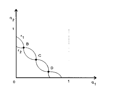
The way to model the possibility of commitments (and related moves like “promises”) is to explicitly include them as actions the players can take. (Schelling (1960) was an early proponent of this view.) We have already seen one example of the value of commitment in our study of the Stackelberg game. which describes a situation where one firm (the “leader”) can commit itself to an output level that the follower is forced to take as given when making its own output decision. Under the typical assumption that each firm’s optimal reaction $r_i\left(q_j\right)$ is a decreasing function of its opponent’s output. the Stackelberg leader’s payoff is higher than in the “Cournot equilibrium” outcome where the two firms choose their output levels simultaneously.
In the Stackelberg example, commitment is achieved simply by moving earlier than the opponent. Although this corresponds to a different extensive form than the simultaneous moves of Cournot competition, the set of “physical actions” is in some sense the same. The search for a way to commit oneself can also lead to the use of actions that would not otherwise have been considered. Classic examples include a general burning his bridges behind him as a commitment not to retreat and Odysseus having himself lashed to the mast and ordering his sailors to plug their ears with wax as a commitment not to go to the Sirens” island. (Note that the natural way to model the Odysseus story is with two “players,” corresponding to ()dysseus before and Odysseus after he is exposed to the Sirens.) Both of these cases correspond to a “total commitment”: Once the bridge is burned, or Odysseus is lashed to the mast and the sailors’ ears are filled with wax, the cost of turning back or escaping from the mast is taken to be infinite. One can also consider partial commitments, which increase the cost of, c.g., turning back without making it infinite.

博弈论代考
经济代写|博弈论代写Game Theory代考|Backward Induction and Subgame Perfection
在Stackelberg博弈中,很容易看出玩家2“应该”怎么玩,因为一旦q_1$固定,玩家2将面临一个简单的决策问题。这让我们能够解出参与人2对于每个q_1$的第二阶段最优选择,然后反向找出参与人1的最优选择。这个算法可以扩展到其他在每个阶段只有一个玩家移动的游戏中。我们说一个多阶段博弈具有完美信息,如果对于每一个阶段$k$和历史$h^k$,只有一个参与者有一个非平凡的选择集一个包含多个元素的选择集而所有其他人都有一个“什么都不做”的单元素选择集举个简单的例子,玩家1在第0、2、4阶段移动,玩家2在第1、3、5阶段移动,以此类推。更一般地说,有些玩家可以连续移动几次,而哪个玩家可以在阶段k中移动可能取决于之前的历史。关键是每个阶段只有一个玩家移动。由于我们假设每个玩家都知道所有对手过去的选择,这意味着在k处移动的单个玩家“完全了解”游戏的所有方面,除了那些将在未来发生的事情。
逆向归纳法可以应用于任何具有完全信息的有限博弈,其中有限意味着阶段的数量是有限的,任何阶段的可行行动的数量也是有限的。算法首先确定最后阶段每个历史的最优选择,也就是说,给定历史,玩家移动时的行动,在达到h^K的条件下,最大化玩家的收益。(可能有不止一个最大化的选择;在这种情况下,逆向归纳允许玩家选择任何最大化者。)然后我们回到第K-1阶段,并确定在那里移动的玩家的最佳行动,因为在第K阶段具有历史$h^K$的移动玩家将采取我们之前确定的行动。算法继续“回滚”,就像解决决策问题一样,直到到达初始阶段。在这一点上,我们已经构建了一个策略概要,并且很容易验证这将最大化玩家的收益,条件是达到$h^{\ mathm {N}}$。(可能有不止一个最大化的选择;在这种情况下,逆向归纳允许玩家选择任何最大化者。)然后我们回到第K-1阶段,并确定在那里移动的玩家的最佳行动,因为在第K阶段具有历史$h^K$的移动玩家将采取我们之前确定的行动。算法继续“回滚”,就像解决决策问题一样,直到到达初始阶段。至此,我们已经构建了一个策略概要,并且很容易验证该概要是纳什均衡。此外,它还有一个很好的属性,即每个玩家的行动在每个可能的历史中都是最优的。
对于两阶段Stackelberg博弈的反向归纳解决方案,即参与人1应该能够预测参与人2在第二阶段的行为,我们认为这是非常有说服力的。在三阶段的游戏中,论证就复杂一些:在第0阶段移动的玩家必须预测在第1阶段移动的玩家能够正确预测在第2阶段移动的玩家的行为,这显然是一个要求更高的假设。在更长的博弈中,逆向归纳法的论证需要相应的更复杂的假设。出于这个原因,逆向归纳论证在“长”游戏中可能不那么有说服力。现在,我们先不讨论反对逆向归纳法的论点;第3.6节更详细地讨论了它的局限性。
经济代写|博弈论代写Game Theory代考|The Value of Commitment and “Time Consistency”
动态游戏分析中反复出现的一个主题是,在许多情况下,玩家可以从以某种方式进行游戏的约束性承诺中获益。在单人游戏中——例如……一个决策问题——这样的承诺不可能有价值,因为玩家在按照承诺进行游戏时可以获得的任何收益都可以在没有承诺的情况下以完全相同的方式进行游戏而获得。但是,如果有不止一个玩家,承诺就会有价值,因为通过承诺自己的特定行动序列,玩家可能会改变对手的玩法。这种承诺的“矛盾”价值与我们在第一章中观察到的密切相关,即玩家可以通过减少自己的行动集或减少某些结果的收益而获得收益,前提是他的对手意识到这种变化。的确,某些形式的承诺可以用这种方式来表示。
为承诺(以及“承诺”之类的相关动作)的可能性建模的方法是明确地将它们作为玩家可以采取的行动。(谢林(1960)是这一观点的早期支持者。)在研究Stackelberg博弈时,我们已经看到了承诺价值的一个例子。它描述了这样一种情况,即一个企业(“领导者”)可以承诺自己的产出水平,而追随者在做出自己的产出决策时被迫采取既定的产出水平。在典型的假设下,每个公司的最优反应$r_i\left(q_j\right)$是其对手产出的递减函数。在“古诺均衡”中,两家企业同时选择各自的产出水平。
在Stackelberg的例子中,承诺只是通过比对手更早行动来实现的。虽然这与古诺竞争的同时运动对应的是一种不同的广泛形式,但“身体动作”的集合在某种意义上是相同的。寻找一种方式来承诺自己也可以导致使用行动,否则不会被考虑。经典的例子包括一位将军烧毁了身后的桥梁,以保证不撤退;奥德修斯把自己绑在桅杆上,命令他的水手用蜡塞住耳朵,以保证不去塞壬的岛。(注意,奥德修斯故事的自然模型是两个“玩家”,对应于()之前的奥德修斯和之后的奥德修斯暴露在塞壬面前。)这两种情况都对应于一种“完全的承诺”:一旦桥被烧毁,或者奥德修斯被绑在桅杆上,水手们的耳朵被蜡填满,回头或逃离桅杆的代价被认为是无限的。我们也可以考虑部分承诺,这增加了成本,例如,回头而不使其无限。

统计代写请认准statistics-lab™. statistics-lab™为您的留学生涯保驾护航。
金融工程代写
金融工程是使用数学技术来解决金融问题。金融工程使用计算机科学、统计学、经济学和应用数学领域的工具和知识来解决当前的金融问题,以及设计新的和创新的金融产品。
非参数统计代写
非参数统计指的是一种统计方法,其中不假设数据来自于由少数参数决定的规定模型;这种模型的例子包括正态分布模型和线性回归模型。
广义线性模型代考
广义线性模型(GLM)归属统计学领域,是一种应用灵活的线性回归模型。该模型允许因变量的偏差分布有除了正态分布之外的其它分布。
术语 广义线性模型(GLM)通常是指给定连续和/或分类预测因素的连续响应变量的常规线性回归模型。它包括多元线性回归,以及方差分析和方差分析(仅含固定效应)。
有限元方法代写
有限元方法(FEM)是一种流行的方法,用于数值解决工程和数学建模中出现的微分方程。典型的问题领域包括结构分析、传热、流体流动、质量运输和电磁势等传统领域。
有限元是一种通用的数值方法,用于解决两个或三个空间变量的偏微分方程(即一些边界值问题)。为了解决一个问题,有限元将一个大系统细分为更小、更简单的部分,称为有限元。这是通过在空间维度上的特定空间离散化来实现的,它是通过构建对象的网格来实现的:用于求解的数值域,它有有限数量的点。边界值问题的有限元方法表述最终导致一个代数方程组。该方法在域上对未知函数进行逼近。[1] 然后将模拟这些有限元的简单方程组合成一个更大的方程系统,以模拟整个问题。然后,有限元通过变化微积分使相关的误差函数最小化来逼近一个解决方案。
tatistics-lab作为专业的留学生服务机构,多年来已为美国、英国、加拿大、澳洲等留学热门地的学生提供专业的学术服务,包括但不限于Essay代写,Assignment代写,Dissertation代写,Report代写,小组作业代写,Proposal代写,Paper代写,Presentation代写,计算机作业代写,论文修改和润色,网课代做,exam代考等等。写作范围涵盖高中,本科,研究生等海外留学全阶段,辐射金融,经济学,会计学,审计学,管理学等全球99%专业科目。写作团队既有专业英语母语作者,也有海外名校硕博留学生,每位写作老师都拥有过硬的语言能力,专业的学科背景和学术写作经验。我们承诺100%原创,100%专业,100%准时,100%满意。
随机分析代写
随机微积分是数学的一个分支,对随机过程进行操作。它允许为随机过程的积分定义一个关于随机过程的一致的积分理论。这个领域是由日本数学家伊藤清在第二次世界大战期间创建并开始的。
时间序列分析代写
随机过程,是依赖于参数的一组随机变量的全体,参数通常是时间。 随机变量是随机现象的数量表现,其时间序列是一组按照时间发生先后顺序进行排列的数据点序列。通常一组时间序列的时间间隔为一恒定值(如1秒,5分钟,12小时,7天,1年),因此时间序列可以作为离散时间数据进行分析处理。研究时间序列数据的意义在于现实中,往往需要研究某个事物其随时间发展变化的规律。这就需要通过研究该事物过去发展的历史记录,以得到其自身发展的规律。
回归分析代写
多元回归分析渐进(Multiple Regression Analysis Asymptotics)属于计量经济学领域,主要是一种数学上的统计分析方法,可以分析复杂情况下各影响因素的数学关系,在自然科学、社会和经济学等多个领域内应用广泛。
MATLAB代写
MATLAB 是一种用于技术计算的高性能语言。它将计算、可视化和编程集成在一个易于使用的环境中,其中问题和解决方案以熟悉的数学符号表示。典型用途包括:数学和计算算法开发建模、仿真和原型制作数据分析、探索和可视化科学和工程图形应用程序开发,包括图形用户界面构建MATLAB 是一个交互式系统,其基本数据元素是一个不需要维度的数组。这使您可以解决许多技术计算问题,尤其是那些具有矩阵和向量公式的问题,而只需用 C 或 Fortran 等标量非交互式语言编写程序所需的时间的一小部分。MATLAB 名称代表矩阵实验室。MATLAB 最初的编写目的是提供对由 LINPACK 和 EISPACK 项目开发的矩阵软件的轻松访问,这两个项目共同代表了矩阵计算软件的最新技术。MATLAB 经过多年的发展,得到了许多用户的投入。在大学环境中,它是数学、工程和科学入门和高级课程的标准教学工具。在工业领域,MATLAB 是高效研究、开发和分析的首选工具。MATLAB 具有一系列称为工具箱的特定于应用程序的解决方案。对于大多数 MATLAB 用户来说非常重要,工具箱允许您学习和应用专业技术。工具箱是 MATLAB 函数(M 文件)的综合集合,可扩展 MATLAB 环境以解决特定类别的问题。可用工具箱的领域包括信号处理、控制系统、神经网络、模糊逻辑、小波、仿真等。