如果你也在 怎样代写图论Graph Theory 这个学科遇到相关的难题，请随时右上角联系我们的24/7代写客服。图论Graph Theory有趣的部分原因在于，图可以用来对某些问题中的情况进行建模。这些问题可以在图表的帮助下进行研究(并可能得到解决)。因此，图形模型在本书中经常出现。然而，图论是数学的一个领域，因此涉及数学思想的研究-概念和它们之间的联系。我们选择包含的主题和结果是因为我们认为它们有趣、重要和/或代表主题。

图论Graph Theory通过熟悉许多过去和现在对图论的发展负责的人，可以增强对图论的欣赏。因此，我们收录了一些关于“图论人士”的有趣评论。因为我们相信这些人是图论故事的一部分，所以我们在文中讨论了他们，而不仅仅是作为脚注。我们常常没有认识到数学是一门有生命的学科。图论是人类创造的，是一门仍在不断发展的学科。

statistics-lab™ 为您的留学生涯保驾护航 在代写图论Graph Theory方面已经树立了自己的口碑, 保证靠谱, 高质且原创的统计Statistics代写服务。我们的专家在代写图论Graph Theory代写方面经验极为丰富，各种代写图论Graph Theory相关的作业也就用不着说。

数学代写|图论作业代写Graph Theory代考|Dominating Set

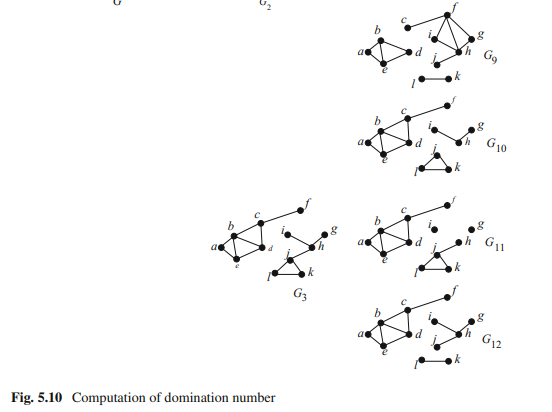
For a graph $G=(V, E)$, a set $D \subseteq V(G)$ of vertices is a dominating set of $G$ if every vertex in $V$ is either in $D$ or adjacent to a vertex of $D$. A dominating set $D$ of $G$ is minimal if $D$ does not properly contain a dominating set of $D$. The vertex set ${b, e, i}$ is a minimal dominating set in the graph in Fig. 5.9. A dominating set $D$ of $G$ is minimum if no other dominating set has fewer vertices than $D$. The cardinality of a minimum dominating set of $G$ is called the domination number of $G$ and denoted by $\gamma(G)$. For the graph in Fig. $5.9 \gamma(G)=2$ and the vertex set ${b, f}$ is a minimum dominating set. We say a vertex in a dominating set dominates itself and all of its neighbors.

The government plans to establish fire stations in a new city in such a way that a locality or one of its neighbor localities will have a fire station. In a graph model of the city, where each vertex represents a locality and each edge represents the neighborhood of two localities, a dominating set gives a feasible solution for the locations of fire stations. If the government wishes to minimize the number of fire stations for budget constraint, a minimum dominating set gives a feasible solution.

Domination of vertices has been studied extensively due its practical applications in scenarios described above [4].

Domination number has a relation with diameter of a graph as we see in the following lemma.

Lemma 5.4.1 Let $G$ be a connected simple graph, $\gamma(G)$ be the domination number of $G$, and $\operatorname{diam}(G)$ be the diameter of $G$. Then
$$
\gamma(G) \geq\left\lceil\frac{\operatorname{diam}(G)+1}{3}\right\rceil .
$$
Proof Let $x$ and $y$ be two vertices of $G$ such that $d(x, y)=\operatorname{diam}(G)=k$, and let $P=u_0(=x), u_1, \ldots, u_k(=y)$ be a path of length $k$ in $G$ from $x$ to $y$. Let $D$ be a domination set of $G$. We now prove that each vertex in $D$ can dominate at most three vertices on $P$. Let $u$ be a vertex in $D$. If $u$ is on $P, u$ can dominate at most three vertices on $P: v$ itself and its (at most) two neighbors. If $u$ is not on $P, u$ can also dominate at most three vertices on $P$ and those vertices must be consecutive on $P$; otherwise, there would exist a path between $x$ and $y$ shorter than $P$, a contradiction to the definition of $\operatorname{diam}(G)$. Therefore, each vertex in $D$ dominates at most three vertices on $P$.

Since the number of vertices on $P$ is $k+1=\operatorname{diam}(G)+1, \gamma(G) \geq\left\lceil\frac{\operatorname{diam}(G)+1}{3}\right\rceil$.

数学代写|图论作业代写Graph Theory代考|Factor of a Graphraceful Labeling

A factor of a graph $G$ is a spanning subgraph of $G$. A $k$-factor is a spanning $k$-regular subgraph. Clearly, a 1-factor is a perfect matching and exists only for graphs with an even number of vertices. A 2 -factor of $G$ is a disjoint union of cycles of $G$ if the 2 -factor is not connected; a connected 2-factor is a Hamiltonian cycle.

We now know Tutte’s condition [8] for 1-factor. A connected component $H$ of a graph is an odd component if $H$ has odd number of vertices. We denote by $o c(G)$ the number of odd components in a graph $G$. The following theorem is from Tutte [8].
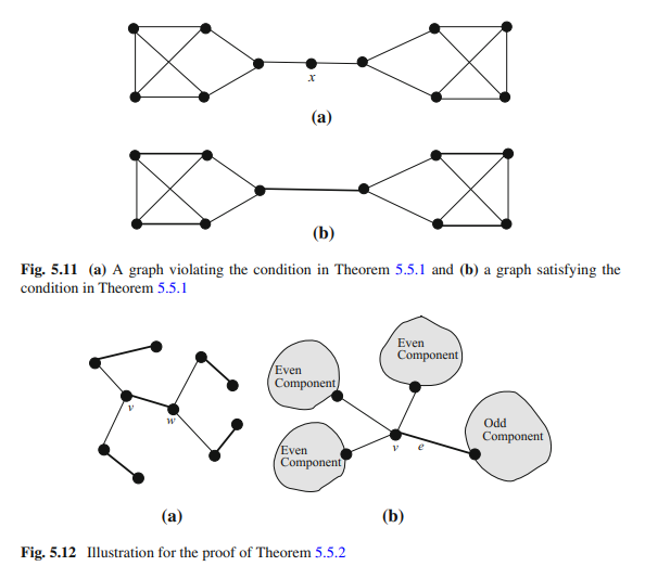
Theorem 5.5.1 A graph $G$ has a l-factor if and only if oc $(G-S) \leq|S|$ for every $S \subseteq V(G)$.

If we delete the vertex $x$ from the graph in Fig.5.11(a), then we get two odd components. Taking $S={x}$, the graph violates the condition in Theorem 5.5.1, and hence it does not have a 1-factor. However, the graph in Fig. 5.11(b) satisfies the condition in Theorem 5.5.1 and it has a 1-factor as shown by thick edges.

We now see an application of Theorem 5.5.1 in the proof of Theorem 5.5.2 (due to Chungphaisan [9]) which gives a necessary and sufficient condition for a tree to have a 1 -factor. The proof presented here is due to Amahashi $[10,11]$.

Theorem 5.5.2 A tree $T$ of even order has a 1 -factor if and only if $o c(T-v)=1$ for every vertex $v$ of $T$.

Proof Assume that $T$ has a 1-factor $F$. Then for every vertex $v$ of $T$, let $w$ be the vertex of $T$ joined to $v$ by an edge of $F$, as illustrated in Fig. 5.12(a). It follows that the component of $T-v$ containing $w$ is odd, and all the other components of $T-v$ are even. Hence $o c(T-v)=1$. Suppose that $o c(T-v)=1$ for every $v \in V(T)$. It is obvious that for each edge $e$ of $T, T-e$ has exactly two components, and both of them are simultaneously odd or even. Define a set $F$ of edges of $T$ as follows: $F={e \in E(T): o c(T-e)=2}$. For every vertex $v$ of $T$, there exists exactly one edge $e$ that is incident with $v$ and satisfies $o c(T-e)=2$ since $T-v$ has exactly one odd component, where $e$ is the edge joining $v$ to this odd component. (See Fig.5.12(b).) Therefore $e$ is an edge of $F$, and thus $F$ is a 1-factor of $G$.

图论代考

数学代写|图论作业代写Graph Theory代考|Dominating Set

对于图$G=(V, E)$，如果$V$中的每个顶点都在$D$或与$D$的顶点相邻，则顶点集$D \subseteq V(G)$就是$G$的支配集。如果$D$没有正确地包含$D$的支配集，那么$G$的支配集$D$就是最小的。顶点集${b, e, i}$是图5.9中的最小支配集。如果没有其他支配集的顶点数少于$D$，那么$G$的支配集$D$是最小的。最小支配集$G$的基数称为$G$的支配数，用$\gamma(G)$表示。对于图$5.9 \gamma(G)=2$中的图，顶点集${b, f}$是最小支配集。我们说支配集中的一个顶点支配它自己和它所有的邻居。

政府计划在新城市设立消防局，在一个地区或附近地区设立一个消防局。在城市图模型中，每个顶点代表一个位置，每条边代表两个位置的邻域，支配集给出了消防站位置的可行解。当政府希望在预算约束下使消防站数量最小化时，最小支配集给出了一个可行解。

由于顶点支配在上述场景中的实际应用，它已被广泛研究[4]。

支配数与图的直径有关系，如下面的引理所示。

设$G$为连通简单图，$\gamma(G)$为$G$的支配数，$\operatorname{diam}(G)$为$G$的直径。然后
$$
\gamma(G) \geq\left\lceil\frac{\operatorname{diam}(G)+1}{3}\right\rceil .
$$
设$x$和$y$为$G$的两个顶点，使得$d(x, y)=\operatorname{diam}(G)=k$;设$P=u_0(=x), u_1, \ldots, u_k(=y)$为$G$从$x$到$y$的一条长度为$k$的路径。设$D$为$G$的支配集。现在我们证明$D$上的每个顶点最多可以支配$P$上的三个顶点。设$u$是$D$的一个顶点。如果$u$在$P, u$上，那么它最多可以支配$P: v$上的三个顶点和它的(最多)两个邻居。如果$u$不在$P, u$也可以支配最多三个顶点的$P$和这些顶点必须是连续的$P$;否则，在$x$和$y$之间会存在一条比$P$短的路径，这与$\operatorname{diam}(G)$的定义相矛盾。因此，$D$中的每个顶点最多支配$P$上的三个顶点。

因为$P$上的顶点数是$k+1=\operatorname{diam}(G)+1, \gamma(G) \geq\left\lceil\frac{\operatorname{diam}(G)+1}{3}\right\rceil$。

数学代写|图论作业代写Graph Theory代考|Factor of a Graphraceful Labeling

图$G$的一个因子是$G$的生成子图。$k$ -因子是生成的$k$ -正则子图。显然，1因子是一种完美匹配，只存在于具有偶数个顶点的图中。如果2因子不连通，则$G$的2因子是$G$的环的不相交并;连通的2因子是一个哈密顿循环。

我们现在知道了Tutte条件[8]的一个因素。如果$H$的顶点数为奇数，则图的连通分量$H$为奇数分量。我们用$o c(G)$表示图$G$中奇数分量的个数。下面的定理来自Tutte[8]。
定理5.5.1图$G$有一个l因子当且仅当oc $(G-S) \leq|S|$对于每一个$S \subseteq V(G)$。

如果我们从图5.11(a)中的图中删除顶点$x$，那么我们得到两个奇数分量。取$S={x}$，图违反定理5.5.1中的条件，因此它不具有1因子。然而，图5.11(b)中的图满足定理5.5.1中的条件，其具有1因子，如粗边所示。

我们现在看到定理5.5.1在定理5.5.2(由于Chungphaisan[9])的证明中的一个应用，定理5.5.2给出了树具有1因子的充分必要条件。这里的证明是由Amahashi $[10,11]$提供的。

定理5.5.2偶阶树$T$有一个1因子当且仅当$o c(T-v)=1$对于$T$的每个顶点$v$。

假设$T$有一个1因子$F$。然后，对于$T$的每个顶点$v$，设$w$为$T$的顶点，并以$F$的边与$v$相连，如图5.12(a)所示。由此可知，$T-v$中包含$w$的分量为奇数，而$T-v$中其他所有分量均为偶数。因此，$o c(T-v)=1$。假设每个$v \in V(T)$对应$o c(T-v)=1$。很明显，对于$T, T-e$的每条边$e$都恰好有两个分量，并且它们同时都是奇数或偶数。定义$T$的边集$F$如下所示:$F={e \in E(T): o c(T-e)=2}$。对于$T$的每个顶点$v$，存在一条与$v$相关且满足$o c(T-e)=2$的边$e$，因为$T-v$正好有一个奇分量，其中$e$是连接$v$和这个奇分量的边。(见图5.12(b)。)因此$e$是$F$的一条边，因此$F$是$G$的一个因子。

统计代写请认准statistics-lab™. statistics-lab™为您的留学生涯保驾护航。

微观经济学代写

微观经济学是主流经济学的一个分支，研究个人和企业在做出有关稀缺资源分配的决策时的行为以及这些个人和企业之间的相互作用。my-assignmentexpert™ 为您的留学生涯保驾护航 在数学Mathematics作业代写方面已经树立了自己的口碑, 保证靠谱, 高质且原创的数学Mathematics代写服务。我们的专家在图论代写Graph Theory代写方面经验极为丰富，各种图论代写Graph Theory相关的作业也就用不着 说。

线性代数代写

线性代数是数学的一个分支，涉及线性方程，如：线性图，如：以及它们在向量空间和通过矩阵的表示。线性代数是几乎所有数学领域的核心。

博弈论代写

现代博弈论始于约翰-冯-诺伊曼（John von Neumann）提出的两人零和博弈中的混合策略均衡的观点及其证明。冯-诺依曼的原始证明使用了关于连续映射到紧凑凸集的布劳威尔定点定理，这成为博弈论和数学经济学的标准方法。在他的论文之后，1944年，他与奥斯卡-莫根斯特恩（Oskar Morgenstern）共同撰写了《游戏和经济行为理论》一书，该书考虑了几个参与者的合作游戏。这本书的第二版提供了预期效用的公理理论，使数理统计学家和经济学家能够处理不确定性下的决策。

微积分代写

微积分，最初被称为无穷小微积分或 “无穷小的微积分”，是对连续变化的数学研究，就像几何学是对形状的研究，而代数是对算术运算的概括研究一样。

它有两个主要分支，微分和积分；微分涉及瞬时变化率和曲线的斜率，而积分涉及数量的累积，以及曲线下或曲线之间的面积。这两个分支通过微积分的基本定理相互联系，它们利用了无限序列和无限级数收敛到一个明确定义的极限的基本概念 。

计量经济学代写

什么是计量经济学？
计量经济学是统计学和数学模型的定量应用，使用数据来发展理论或测试经济学中的现有假设，并根据历史数据预测未来趋势。它对现实世界的数据进行统计试验，然后将结果与被测试的理论进行比较和对比。

根据你是对测试现有理论感兴趣，还是对利用现有数据在这些观察的基础上提出新的假设感兴趣，计量经济学可以细分为两大类：理论和应用。那些经常从事这种实践的人通常被称为计量经济学家。

Matlab代写

MATLAB 是一种用于技术计算的高性能语言。它将计算、可视化和编程集成在一个易于使用的环境中，其中问题和解决方案以熟悉的数学符号表示。典型用途包括：数学和计算算法开发建模、仿真和原型制作数据分析、探索和可视化科学和工程图形应用程序开发，包括图形用户界面构建MATLAB 是一个交互式系统，其基本数据元素是一个不需要维度的数组。这使您可以解决许多技术计算问题，尤其是那些具有矩阵和向量公式的问题，而只需用 C 或 Fortran 等标量非交互式语言编写程序所需的时间的一小部分。MATLAB 名称代表矩阵实验室。MATLAB 最初的编写目的是提供对由 LINPACK 和 EISPACK 项目开发的矩阵软件的轻松访问，这两个项目共同代表了矩阵计算软件的最新技术。MATLAB 经过多年的发展，得到了许多用户的投入。在大学环境中，它是数学、工程和科学入门和高级课程的标准教学工具。在工业领域，MATLAB 是高效研究、开发和分析的首选工具。MATLAB 具有一系列称为工具箱的特定于应用程序的解决方案。对于大多数 MATLAB 用户来说非常重要，工具箱允许您学习和应用专业技术。工具箱是 MATLAB 函数（M 文件）的综合集合，可扩展 MATLAB 环境以解决特定类别的问题。可用工具箱的领域包括信号处理、控制系统、神经网络、模糊逻辑、小波、仿真等。