如果你也在 怎样代写金融计量经济学Financial Econometrics 这个学科遇到相关的难题，请随时右上角联系我们的24/7代写客服。金融计量经济学Financial Econometrics是使用统计方法来发展理论或检验经济学或金融学的现有假设。计量经济学依靠的是回归模型和无效假设检验等技术。计量经济学也可用于尝试预测未来的经济或金融趋势。

金融计量经济学Financial Econometrics的一个基本工具是多元线性回归模型。计量经济学理论使用统计理论和数理统计来评估和发展计量经济学方法。计量经济学家试图找到具有理想统计特性的估计器，包括无偏性、效率和一致性。应用计量经济学使用理论计量经济学和现实世界的数据来评估经济理论，开发计量经济学模型，分析经济历史和预测。

statistics-lab™ 为您的留学生涯保驾护航 在代写计量经济学Econometrics方面已经树立了自己的口碑, 保证靠谱, 高质且原创的统计Statistics代写服务。我们的专家在代写计量经济学Econometrics代写方面经验极为丰富，各种代写计量经济学Econometrics相关的作业也就用不着说。

经济代写|计量经济学代写Econometrics代考|Univariate Properties of the Data

Trend breaks appear to be prevalent in macroeconomic time series, and unit root tests therefore need to make allowance for these if they are to avoid the serious effects that unmodeled trend breaks have on power. ${ }^{16}$ Consequently, when testing for a unit root it has become a matter of regular practice to allow for this kind of deterministic structural change.

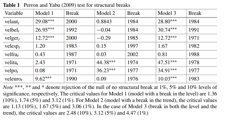
In order to avoid this pitfall, we run tests to assess whether structural breaks are present in the series. This testing problem has been addressed by Perron and Yabu (2009), who define a test statistic that is based on a quasi-GLS approach using an autoregression for the noise component, with a truncation to 1 when the sum of the autoregressive coefficients is in some neighborhood of 1 , along with a bias correction. For given break dates, one constructs the $F$-test (Exp $\left.-W_{F S}\right)$ for the null hypothesis of no structural change in the deterministic components. The final statistic uses the Exp functional of Andrews and Ploberger (1994). Perron and Yabu (2009) specify three different models depending on whether the structural break only affects the level (Model I), the slope of the trend (Model II) or the level and the slope of the time trend (Model III). The computation of these statistics, which are available in Table 1 , shows that we find more evidence against the null hypothesis of no structural break with Model III.

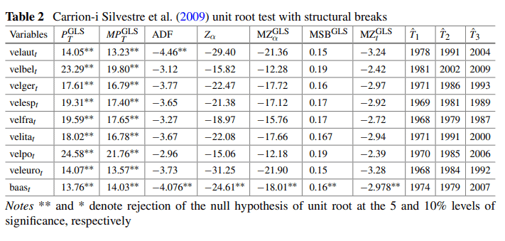
The analysis shows instabilities in the money velocity for all the countries with two exceptions, Spain and France. Therefore, in a second step, we have computed the unit root test statistics in Carrion-i Silvestre et al. (2009). The unit root tests in Carrion-i Silvestre et al. (2009) allow for multiple structural breaks under both the null and alternative hypotheses which make especially suitable for our purpose, since we have obtained evidence in favor of the presence of structural breaks regardless of their order of integration. The results of all these statistics are reported in Table 3. As can be seen, the unit root tests proposed by Carrion-i Silvestre et al. (2009) led to the non-rejection of the null hypothesis of a unit root in most of cases at the $5 \%$ level of

经济代写|计量经济学代写Econometrics代考|M3 Velocity Panel TVP Model Estimation

In this subsection, we present the results from the estimation of the model for the time-varying determinants of M3 velocity. The estimates have been obtained by using a Gauss code that extends the traditional approach by Hamilton (1994b) and includes all the elements of the model presented in Sect. 3.2. The results for the maximum likelihood estimation of the elements of the hyper-parameter vector are reported in Table 5 , for both the measurement equation and the state-transition equations.

The first part of Table 5 displays the hyper-parameters for the “measurement equation” in Eq. (30), estimated for our panel including the following Eurozone members: Austria, Belgium, Germany, Spain, France, Italy and Portugal. The last column presents the results for the model when estimated for the Eurozone as a whole. The estimated country-specific fixed parameters are reported for the measurement equation, where $\beta_{0 i}$ is the fixed-mean intercept, $\beta_{1 i}$ is the fixed-mean parameter for the $\log$ of the permanent component of real GNI per capita $\left(\operatorname{logGNIpc}{ }^p\right), \beta_{2 i}$ is the fixed coefficient for the lagged dependent variable, $\left(\operatorname{lnM} 3 \mathrm{~V}{i, t-1}\right)$, and $\beta{3 i}$ is the mean parameter for baaspread ${ }t$, our measure of global risk aversion. The table also displays the estimated common mean fixed parameters $\beta_4$ and $\beta_5$, for the expected inflation $\left(\pi{i, t}^e\right)$, and the real short-term interest rate, $\left(\operatorname{rstir}_{i, t}\right)$, respectively.

The rest of the table includes the estimated hyper-parameters for the “state-update equation” in Eq. (31) that contribute to explain the transition of the country-specific varying parameter vector, $\xi_{1, i, t}$, which stands for the varying component of the parameter for $\operatorname{lnGNIpc_{i,t}^{p}}$. Each unobserved component follows an autoregressive process estimated with a common autoregressive parameter $\phi_1$. Finally, our state-space equation also includes control instruments that drive the varying components of both parameters: GNIpc ${ }{i, t}^{c+}$ and GNIpc ${ }{i, t}^c$. They capture the asymmetric impact of positive and negative deviations from the trend of GNI per capita, calculated as the logarithm of the GNI-to-GNI trend ratio. These control instruments enter as country-specific.

计量经济学代考

经济代写|计量经济学代写Econometrics代考|Univariate Properties of the Data

趋势中断似乎在宏观经济时间序列中很普遍，因此，如果要避免未建模的趋势中断对功率的严重影响，单位根检验就需要考虑到这些。${}^{16}$因此，在测试单位根时，允许这种确定性结构变化已成为常规实践的问题。

为了避免这个陷阱，我们运行测试来评估系列中是否存在结构中断。Perron和Yabu(2009)已经解决了这个测试问题，他们定义了一个基于准gls方法的测试统计量，该方法使用噪声分量的自回归，当自回归系数的总和在1附近时截断为1，并进行偏差校正。对于给定的休息日期，构造$F$-test (Exp $\left)。-W_{F S}\right)$表示确定性成分无结构变化的零假设。最后的统计使用Andrews和plobberger(1994)的Exp函数。Perron和Yabu(2009)根据结构断裂是只影响水平(模型一)、趋势斜率(模型二)还是水平和时间趋势斜率(模型三)，指定了三种不同的模型。对这些统计量的计算(见表1)表明，我们在模型三中发现了更多反对无结构断裂原假设的证据。

分析显示，除西班牙和法国两个国家外，所有国家的货币流通速度都不稳定。因此，在第二步中，我们计算了Carrion-i Silvestre et al.(2009)的单位根检验统计量。Carrion-i Silvestre等人(2009)的单位根检验允许在零假设和替代假设下存在多个结构断裂，这特别适合我们的目的，因为我们已经获得了支持结构断裂存在的证据，无论其整合顺序如何。表3报告了所有这些统计数据的结果。可以看出，Carrion-i Silvestre等人(2009)提出的单位根检验导致在大多数情况下，在5%显著性水平下，单位根的零假设不被拒绝。${}^{17}$我们的结论是，所考虑的国家的收入速度变量在水平和大多数情况下都具有单位根。

经济代写|计量经济学代写Econometrics代考|M3 Velocity Panel TVP Model Estimation

在本节中，我们给出了M3速度时变决定因素的模型估计结果。估计是通过使用高斯代码获得的，该代码扩展了Hamilton (1994b)的传统方法，并包括第3.2节中提出的模型的所有元素。表5报告了测量方程和状态转移方程的超参数向量元素的最大似然估计结果。

表5的第一部分显示了Eq.(30)中“测量方程”的超参数，我们的小组估计包括以下欧元区成员国:奥地利、比利时、德国、西班牙、法国、意大利和葡萄牙。最后一列给出了对整个欧元区进行估计后的模型结果。测量方程报告了估计的特定国家固定参数，其中$\beta_{0 i}$是固定平均截距，$\beta_{1 i}$是实际人均国民总收入永久成分$\log$的固定平均参数$\left(\operatorname{logGNIpc}{ }^p\right), \beta_{2 i}$是滞后因变量$\left(\operatorname{lnM} 3 \mathrm{~V}{i, t-1}\right)$的固定系数，$\beta{3 i}$是baspread ${ }t$的平均参数，我们衡量全球风险厌恶程度。该表还分别显示了预期通货膨胀$\left(\pi{i, t}^e\right)$和实际短期利率$\left(\operatorname{rstir}_{i, t}\right)$的估计共同平均固定参数$\beta_4$和$\beta_5$。

表的其余部分包括公式(31)中“状态更新方程”的估计超参数，这些超参数有助于解释特定于国家的变化参数向量$\xi_{1, i, t}$的转变，代表$\operatorname{lnGNIpc_{i,t}^{p}}$参数的变化部分。每个未观察到的成分都遵循一个自回归过程，用一个共同的自回归参数$\phi_1$估计。最后，我们的状态空间方程还包括驱动两个参数的不同组件的控制工具:GNIpc ${ }{i, t}^{c+}$和GNIpc ${ }{i, t}^c$。它们反映了与人均国民总收入趋势正偏差和负偏差的不对称影响，以国民总收入与国民总收入趋势比率的对数计算。这些控制文书根据具体国家的情况进入。

统计代写请认准statistics-lab™. statistics-lab™为您的留学生涯保驾护航。

金融工程代写

金融工程是使用数学技术来解决金融问题。金融工程使用计算机科学、统计学、经济学和应用数学领域的工具和知识来解决当前的金融问题，以及设计新的和创新的金融产品。

非参数统计代写

非参数统计指的是一种统计方法，其中不假设数据来自于由少数参数决定的规定模型；这种模型的例子包括正态分布模型和线性回归模型。

广义线性模型代考

广义线性模型（GLM）归属统计学领域，是一种应用灵活的线性回归模型。该模型允许因变量的偏差分布有除了正态分布之外的其它分布。

术语 广义线性模型（GLM）通常是指给定连续和/或分类预测因素的连续响应变量的常规线性回归模型。它包括多元线性回归，以及方差分析和方差分析（仅含固定效应）。

有限元方法代写

有限元方法（FEM）是一种流行的方法，用于数值解决工程和数学建模中出现的微分方程。典型的问题领域包括结构分析、传热、流体流动、质量运输和电磁势等传统领域。

有限元是一种通用的数值方法，用于解决两个或三个空间变量的偏微分方程（即一些边界值问题）。为了解决一个问题，有限元将一个大系统细分为更小、更简单的部分，称为有限元。这是通过在空间维度上的特定空间离散化来实现的，它是通过构建对象的网格来实现的：用于求解的数值域，它有有限数量的点。边界值问题的有限元方法表述最终导致一个代数方程组。该方法在域上对未知函数进行逼近。[1] 然后将模拟这些有限元的简单方程组合成一个更大的方程系统，以模拟整个问题。然后，有限元通过变化微积分使相关的误差函数最小化来逼近一个解决方案。

tatistics-lab作为专业的留学生服务机构，多年来已为美国、英国、加拿大、澳洲等留学热门地的学生提供专业的学术服务，包括但不限于Essay代写，Assignment代写，Dissertation代写，Report代写，小组作业代写，Proposal代写，Paper代写，Presentation代写，计算机作业代写，论文修改和润色，网课代做，exam代考等等。写作范围涵盖高中，本科，研究生等海外留学全阶段，辐射金融，经济学，会计学，审计学，管理学等全球99%专业科目。写作团队既有专业英语母语作者，也有海外名校硕博留学生，每位写作老师都拥有过硬的语言能力，专业的学科背景和学术写作经验。我们承诺100%原创，100%专业，100%准时，100%满意。

随机分析代写

随机微积分是数学的一个分支，对随机过程进行操作。它允许为随机过程的积分定义一个关于随机过程的一致的积分理论。这个领域是由日本数学家伊藤清在第二次世界大战期间创建并开始的。

时间序列分析代写

随机过程，是依赖于参数的一组随机变量的全体，参数通常是时间。 随机变量是随机现象的数量表现，其时间序列是一组按照时间发生先后顺序进行排列的数据点序列。通常一组时间序列的时间间隔为一恒定值（如1秒，5分钟，12小时，7天，1年），因此时间序列可以作为离散时间数据进行分析处理。研究时间序列数据的意义在于现实中，往往需要研究某个事物其随时间发展变化的规律。这就需要通过研究该事物过去发展的历史记录，以得到其自身发展的规律。

回归分析代写

多元回归分析渐进（Multiple Regression Analysis Asymptotics）属于计量经济学领域，主要是一种数学上的统计分析方法，可以分析复杂情况下各影响因素的数学关系，在自然科学、社会和经济学等多个领域内应用广泛。

MATLAB代写

MATLAB 是一种用于技术计算的高性能语言。它将计算、可视化和编程集成在一个易于使用的环境中，其中问题和解决方案以熟悉的数学符号表示。典型用途包括：数学和计算算法开发建模、仿真和原型制作数据分析、探索和可视化科学和工程图形应用程序开发，包括图形用户界面构建MATLAB 是一个交互式系统，其基本数据元素是一个不需要维度的数组。这使您可以解决许多技术计算问题，尤其是那些具有矩阵和向量公式的问题，而只需用 C 或 Fortran 等标量非交互式语言编写程序所需的时间的一小部分。MATLAB 名称代表矩阵实验室。MATLAB 最初的编写目的是提供对由 LINPACK 和 EISPACK 项目开发的矩阵软件的轻松访问，这两个项目共同代表了矩阵计算软件的最新技术。MATLAB 经过多年的发展，得到了许多用户的投入。在大学环境中，它是数学、工程和科学入门和高级课程的标准教学工具。在工业领域，MATLAB 是高效研究、开发和分析的首选工具。MATLAB 具有一系列称为工具箱的特定于应用程序的解决方案。对于大多数 MATLAB 用户来说非常重要，工具箱允许您学习和应用专业技术。工具箱是 MATLAB 函数（M 文件）的综合集合，可扩展 MATLAB 环境以解决特定类别的问题。可用工具箱的领域包括信号处理、控制系统、神经网络、模糊逻辑、小波、仿真等。

R语言代写	问卷设计与分析代写
PYTHON代写	回归分析与线性模型代写
MATLAB代写	方差分析与试验设计代写
STATA代写	机器学习/统计学习代写
SPSS代写	计量经济学代写
EVIEWS代写	时间序列分析代写
EXCEL代写	深度学习代写
SQL代写	各种数据建模与可视化代写

如果你也在 怎样代写金融计量经济学Financial Econometrics 这个学科遇到相关的难题，请随时右上角联系我们的24/7代写客服。金融计量经济学Financial Econometrics是使用统计方法来发展理论或检验经济学或金融学的现有假设。计量经济学依靠的是回归模型和无效假设检验等技术。计量经济学也可用于尝试预测未来的经济或金融趋势。

金融计量经济学Financial Econometrics的一个基本工具是多元线性回归模型。计量经济学理论使用统计理论和数理统计来评估和发展计量经济学方法。计量经济学家试图找到具有理想统计特性的估计器，包括无偏性、效率和一致性。应用计量经济学使用理论计量经济学和现实世界的数据来评估经济理论，开发计量经济学模型，分析经济历史和预测。

statistics-lab™ 为您的留学生涯保驾护航 在代写计量经济学Econometrics方面已经树立了自己的口碑, 保证靠谱, 高质且原创的统计Statistics代写服务。我们的专家在代写计量经济学Econometrics代写方面经验极为丰富，各种代写计量经济学Econometrics相关的作业也就用不着说。

经济代写|计量经济学代写Econometrics代考|Classical Test Approaches

We use three left-tailed unit root tests (the ADF, Phillips-Perron, and DF-GLS) that are popular univariate tests in economic and financial research. These tests investigate the null hypothesis that the price-to-rent ratio in levels follows the unit root process (I(1)), and a rejection of this null provides evidence of stationarity in this ratio, and thus cointegration between housing prices and rents. Therefore, a failure to reject this null hypothesis indicates that rents cannot explain the long-term housing price movements, thereby suggesting the presence of mild bubbles. We conduct these tests for the ratios in levels and first differences in order to check the order of integration.
Table 3 summarizes the test statistics for the Euro area, Japan, the UK, and the USA. The results suggest that these ratios follow the unit root process. Using the $5 \%$ critical values, we often fail to reject the null hypothesis for the data in levels, but can do so for the differenced data. Therefore, we conclude that mild bubbles existed in all countries, suggesting that rental increases are not always associated with housing price inflation, and there must be some periods when housing prices deviate substantially from the trend in rentals. Obviously, these tests preclude a possibility of explosive bubbles, and moreover, we need to pay attention to the composition of economic fundamentals. However, these outcomes are consistent with our expectations that all housing markets experienced chaotic moments during our sample period.
The potential non-stationary periods identified by the classical method are shaded in Fig. 3. We present two graphs for each country, and the upper figures (denoted as OLS estimates) are obtained from the classical method. As explained earlier, a drawback of this approach is the lack of statistical power to differentiate between hypotheses and that it allows for negative bubbles. For consistency with the standard phenomenon of financial bubbles, we should consider only the positive bubbles (above the horizontal line) as relevant to financial bubbles. Thus, only positive bubble periods are highlighted in gray in this figure and are potential bubble periods because these classical tests are not designed to identify the exact periods of bubbles while they give us evidence of mild bubbles during the sample period. ${ }^5$

经济代写|计量经济学代写Econometrics代考|Explosive Test Approaches

Next, we conduct explosive unit root tests for each country and for a group of countries. From the classical tests, we already know that the price-to-rent ratio is nonstationary and, in fact, implies the presence of mild bubbles. However, when it is not known, we propose the following general steps to reach a conclusion. In short, explosive unit root tests should be conducted if and only if the classical approaches show the data $(y)$ to be a non-stationary process.
A general approach to identify financial bubbles

1. Use the classical approaches to check for the presence of tranquil periods
2. If the null hypothesis of $I(1)$ cannot be rejected, then go to Step 3; otherwise, conclude that the housing market is tranquil.
3. Conduct the explosive bubble tests. If the null hypothesis of these tests is rejected, then conclude the presence of explosive bubbles; otherwise, conclude the presence of mild bubbles in the housing market.

Failing to reject the null hypothesis that price-to-rent ratios are $I(1)$ by the classical tests, we eliminated the possibility of market tranquility and thus conduct explosive unit root tests for each market. Table 4 summarizes the results from the right-tailed tests (RADF, SADF, and GSADF) for each country. The null hypothesis of these tests is consistent with our finding of a random walk price-to-rent ratio from the classical tests. The explosive test results differ somewhat by test type, but the null hypothesis is rejected frequently using the $p$-values obtained from 1000 replications, which is evidence in favor of explosive bubbles in all markets. The results from the GSADF are also depicted in Fig. 4. GSADF statistics greater than 95\% critical values suggest the presence of explosive bubbles, which are also shaded in this figure, and generally identify explosive bubble periods when housing prices are high. The timing and duration of explosive bubbles differ among countries, but many countries seemed to experience explosive bubbles before the Lehman Brothers collapse in September 2018. The presence of real estate markets is consistent with the results from the classical approaches, but here we have evidence of explosive bubbles, which the classical approach cannot capture.

计量经济学代考

经济代写|计量经济学代写Econometrics代考|Classical Test Approaches

我们使用了三个左尾单位根检验(ADF、Phillips-Perron和DF-GLS)，这是经济和金融研究中常用的单变量检验。这些检验研究了原假设，即水平上的房价与租金比率遵循单位根过程(I(1))，拒绝这个null提供了该比率平稳性的证据，从而证明了房价和租金之间的协整。因此，未能拒绝这一零假设表明租金不能解释长期房价变动，从而表明存在温和泡沫。我们对水平和第一差的比率进行这些测试，以检查积分的顺序。
表3总结了欧元区、日本、英国和美国的测试统计数据。结果表明，这些比率遵循单位根过程。使用$5 \%$临界值，我们通常无法拒绝水平数据的零假设，但可以对差异数据这样做。因此，我们得出结论，所有国家都存在温和泡沫，这表明租金上涨并不总是与房价通胀相关，而且一定有一些时期房价大幅偏离租金趋势。显然，这些测试排除了泡沫爆裂的可能性，此外，我们需要关注经济基本面的构成。然而，这些结果与我们的预期一致，即在我们的样本期间，所有房地产市场都经历了混乱的时刻。
通过经典方法确定的潜在非平稳周期在图3中被阴影显示。我们为每个国家提供了两个图表，上面的数字(表示为OLS估计)是从经典方法获得的。如前所述，这种方法的缺点是缺乏区分假设的统计能力，并且它允许负泡沫。为了与金融泡沫的标准现象保持一致，我们应该只考虑正泡沫(水平线以上)与金融泡沫相关。因此，在此图中，只有积极的泡沫时期以灰色突出显示，并且是潜在的泡沫时期，因为这些经典测试不是为了确定泡沫的确切时期而设计的，而它们在样本期间为我们提供了温和泡沫的证据。${} ^ 5美元

经济代写|计量经济学代写Econometrics代考|Explosive Test Approaches

接下来，我们对每个国家和一组国家进行爆炸单位根测试。从经典测试中，我们已经知道租售比是非平稳的，事实上，这意味着存在温和的泡沫。然而，当它是未知的，我们建议以下一般步骤来得出结论。简而言之，当且仅当经典方法表明数据$(y)$是一个非平稳过程时，应进行爆炸单位根试验。
识别金融泡沫的一般方法

使用经典的方法来检查平静时期的存在

如果不能拒绝$I(1)$的零假设，则转到步骤3;否则，得出的结论是房地产市场是平静的。

进行爆炸气泡试验。如果这些检验的零假设被拒绝，则得出爆炸性气泡存在的结论;否则，就得出房地产市场存在温和泡沫的结论。

由于经典检验未能拒绝价租比为$I(1)$的零假设，我们排除了市场平静的可能性，从而对每个市场进行爆炸性单位根检验。表4总结了每个国家的右尾检验(RADF、SADF和GSADF)的结果。这些检验的零假设与我们从经典检验中发现的随机游走价租比一致。爆炸性测试结果因测试类型而有所不同，但使用从1000次重复中获得的p值经常拒绝原假设，这是支持所有市场中爆炸性泡沫的证据。图4也描述了GSADF的结果。GSADF统计数据大于95%的临界值表明存在爆炸性泡沫，这在图中也是阴影，并且通常在房价高企时识别爆炸性泡沫时期。爆炸性泡沫的时间和持续时间因国家而异，但在2018年9月雷曼兄弟破产之前，许多国家似乎都经历了爆炸性泡沫。房地产市场的存在与经典方法的结果是一致的，但这里我们有爆炸性泡沫的证据，这是经典方法无法捕捉到的。以上翻译结果来自有道神经网络翻译（YNMT）· 通用场景

统计代写请认准statistics-lab™. statistics-lab™为您的留学生涯保驾护航。

金融工程代写

金融工程是使用数学技术来解决金融问题。金融工程使用计算机科学、统计学、经济学和应用数学领域的工具和知识来解决当前的金融问题，以及设计新的和创新的金融产品。

非参数统计代写

非参数统计指的是一种统计方法，其中不假设数据来自于由少数参数决定的规定模型；这种模型的例子包括正态分布模型和线性回归模型。

广义线性模型代考

广义线性模型（GLM）归属统计学领域，是一种应用灵活的线性回归模型。该模型允许因变量的偏差分布有除了正态分布之外的其它分布。

术语 广义线性模型（GLM）通常是指给定连续和/或分类预测因素的连续响应变量的常规线性回归模型。它包括多元线性回归，以及方差分析和方差分析（仅含固定效应）。

有限元方法代写

有限元方法（FEM）是一种流行的方法，用于数值解决工程和数学建模中出现的微分方程。典型的问题领域包括结构分析、传热、流体流动、质量运输和电磁势等传统领域。

有限元是一种通用的数值方法，用于解决两个或三个空间变量的偏微分方程（即一些边界值问题）。为了解决一个问题，有限元将一个大系统细分为更小、更简单的部分，称为有限元。这是通过在空间维度上的特定空间离散化来实现的，它是通过构建对象的网格来实现的：用于求解的数值域，它有有限数量的点。边界值问题的有限元方法表述最终导致一个代数方程组。该方法在域上对未知函数进行逼近。[1] 然后将模拟这些有限元的简单方程组合成一个更大的方程系统，以模拟整个问题。然后，有限元通过变化微积分使相关的误差函数最小化来逼近一个解决方案。

tatistics-lab作为专业的留学生服务机构，多年来已为美国、英国、加拿大、澳洲等留学热门地的学生提供专业的学术服务，包括但不限于Essay代写，Assignment代写，Dissertation代写，Report代写，小组作业代写，Proposal代写，Paper代写，Presentation代写，计算机作业代写，论文修改和润色，网课代做，exam代考等等。写作范围涵盖高中，本科，研究生等海外留学全阶段，辐射金融，经济学，会计学，审计学，管理学等全球99%专业科目。写作团队既有专业英语母语作者，也有海外名校硕博留学生，每位写作老师都拥有过硬的语言能力，专业的学科背景和学术写作经验。我们承诺100%原创，100%专业，100%准时，100%满意。

随机分析代写

随机微积分是数学的一个分支，对随机过程进行操作。它允许为随机过程的积分定义一个关于随机过程的一致的积分理论。这个领域是由日本数学家伊藤清在第二次世界大战期间创建并开始的。

时间序列分析代写

随机过程，是依赖于参数的一组随机变量的全体，参数通常是时间。 随机变量是随机现象的数量表现，其时间序列是一组按照时间发生先后顺序进行排列的数据点序列。通常一组时间序列的时间间隔为一恒定值（如1秒，5分钟，12小时，7天，1年），因此时间序列可以作为离散时间数据进行分析处理。研究时间序列数据的意义在于现实中，往往需要研究某个事物其随时间发展变化的规律。这就需要通过研究该事物过去发展的历史记录，以得到其自身发展的规律。

回归分析代写

多元回归分析渐进（Multiple Regression Analysis Asymptotics）属于计量经济学领域，主要是一种数学上的统计分析方法，可以分析复杂情况下各影响因素的数学关系，在自然科学、社会和经济学等多个领域内应用广泛。

MATLAB代写

MATLAB 是一种用于技术计算的高性能语言。它将计算、可视化和编程集成在一个易于使用的环境中，其中问题和解决方案以熟悉的数学符号表示。典型用途包括：数学和计算算法开发建模、仿真和原型制作数据分析、探索和可视化科学和工程图形应用程序开发，包括图形用户界面构建MATLAB 是一个交互式系统，其基本数据元素是一个不需要维度的数组。这使您可以解决许多技术计算问题，尤其是那些具有矩阵和向量公式的问题，而只需用 C 或 Fortran 等标量非交互式语言编写程序所需的时间的一小部分。MATLAB 名称代表矩阵实验室。MATLAB 最初的编写目的是提供对由 LINPACK 和 EISPACK 项目开发的矩阵软件的轻松访问，这两个项目共同代表了矩阵计算软件的最新技术。MATLAB 经过多年的发展，得到了许多用户的投入。在大学环境中，它是数学、工程和科学入门和高级课程的标准教学工具。在工业领域，MATLAB 是高效研究、开发和分析的首选工具。MATLAB 具有一系列称为工具箱的特定于应用程序的解决方案。对于大多数 MATLAB 用户来说非常重要，工具箱允许您学习和应用专业技术。工具箱是 MATLAB 函数（M 文件）的综合集合，可扩展 MATLAB 环境以解决特定类别的问题。可用工具箱的领域包括信号处理、控制系统、神经网络、模糊逻辑、小波、仿真等。

R语言代写	问卷设计与分析代写
PYTHON代写	回归分析与线性模型代写
MATLAB代写	方差分析与试验设计代写
STATA代写	机器学习/统计学习代写
SPSS代写	计量经济学代写
EVIEWS代写	时间序列分析代写
EXCEL代写	深度学习代写
SQL代写	各种数据建模与可视化代写

如果你也在 怎样代写金融计量经济学Financial Econometrics 这个学科遇到相关的难题，请随时右上角联系我们的24/7代写客服。金融计量经济学Financial Econometrics是使用统计方法来发展理论或检验经济学或金融学的现有假设。计量经济学依靠的是回归模型和无效假设检验等技术。计量经济学也可用于尝试预测未来的经济或金融趋势。

金融计量经济学Financial Econometrics的一个基本工具是多元线性回归模型。计量经济学理论使用统计理论和数理统计来评估和发展计量经济学方法。计量经济学家试图找到具有理想统计特性的估计器，包括无偏性、效率和一致性。应用计量经济学使用理论计量经济学和现实世界的数据来评估经济理论，开发计量经济学模型，分析经济历史和预测。

statistics-lab™ 为您的留学生涯保驾护航 在代写计量经济学Econometrics方面已经树立了自己的口碑, 保证靠谱, 高质且原创的统计Statistics代写服务。我们的专家在代写计量经济学Econometrics代写方面经验极为丰富，各种代写计量经济学Econometrics相关的作业也就用不着说。

经济代写|计量经济学代写Econometrics代考|The Theoretical Concept of Rational Bubbles

The main objective of this study is to review statistical methods, but it is still important to understand the underlying economic theory of financial bubbles in order to specify a composition of statistical models. As discussed, recent research casts doubt on the rationality of investors, but many economic analyses maintain this assumption and it is often explained using the present value model (PVM). The rationality assumption prevails in academic research largely for convenience; it is easier to model rational behaviors than irrational ones. Survey data on investors’ expectations are the best source of information about investors’ expectations, but in the absence of survey data for a comprehensive number of countries and infrequent dissemination of survey data, we also maintain the rationality assumption.

According to the PVM, rational bubbles are defined as sizable and persistent deviations from economic fundamentals and follow a non-stationary process in a statistical sense. Based on the definition of asset returns or returns on real estate $\left(r_{t+1}=\left(P_{t+1}+D_{t+1}\right) / P_t-1\right)$, the PVM suggests that the contemporaneous prices $\left(P_t\right)$ will be determined by the expected value of future economic fundamentals $(D)$ and prices:
$$
P_t=E_t\left[\frac{P_{t+1}+D_{t+1}}{1+r_{t+1}}\right]
$$
where $t$ denotes time $(t=1, \ldots, T)$ and $E$ is an expectation operator. $D$ is an economic fundamental, such as dividend payments in equity analyses or rental costs in housing analyses. Solving Eq. (1) forwardly and using the law of iterated expectations, we can obtain Eq. (2):
$$
P_t=E_t\left[\sum_{h=0}^{\infty}\left(\prod_{k=0}^h\left(\frac{1}{1+r_{t+k}}\right)\right) D_{t+h}+\lim {h \rightarrow \infty} \prod{k=0}^h\left(\frac{1}{1+r_{t+k}}\right) P_{t+h}\right]
$$

经济代写|计量经济学代写Econometrics代考|Econometric Methods

Econometricians proposed many statistical methods, with statistical hypotheses that seem designed to be suitable from their perspectives. Consequently, some approaches were developed to look for tranquil periods, while others investigate financial bubbles. Unlike previous studies, we make a clear distinction between statistical approaches to determine tranquil and bubble periods. This distinction is important since differences in the statistical hypotheses can explain the different results from these two approaches. In this section, we will clarify these two approaches using popular statistical specifications in studies of bubbles.

To investigate the theoretical model and predictions in Eq. (2) quantitatively, previous studies often focused on a single market utilizing time series methods. These statistical methods are one-tailed tests, but can be broadly categorized into left- and right-tailed approaches according to their alternative hypotheses. The lefttailed test is classical and is designed to look for cointegration between prices and economic fundamentals, and thus revealing tranquil periods. As an extension, we also propose a nonlinear approach that can be classified into a group of left-tailed tests. On the other hand, the right-tailed test, which has become popular, is an approach to identify explosive bubbles.

计量经济学代考

经济代写|计量经济学代写Econometrics代考|The Theoretical Concept of Rational Bubbles

本研究的主要目的是回顾统计方法，但为了明确统计模型的组成，了解金融泡沫的潜在经济理论仍然很重要。如前所述，最近的研究对投资者的合理性提出了质疑，但许多经济分析坚持这一假设，并经常使用现值模型(PVM)来解释。理性假设在学术研究中盛行，很大程度上是为了方便;理性行为比非理性行为更容易建模。关于投资者预期的调查数据是了解投资者预期的最佳信息来源，但在缺乏全面数量的国家调查数据和调查数据不经常传播的情况下，我们也保持了合理性假设。

根据PVM，理性泡沫被定义为与经济基本面的大规模持续偏离，并遵循统计学意义上的非平稳过程。根据资产收益或房地产收益$\left(r_{t+1}=\left(P_{t+1}+D_{t+1}\right) / P_t-1\right)$的定义，PVM认为同期价格$\left(P_t\right)$将由未来经济基本面$(D)$和价格的期望值决定:
$$
P_t=E_t\left[\frac{P_{t+1}+D_{t+1}}{1+r_{t+1}}\right]
$$
其中$t$表示时间$(t=1, \ldots, T)$, $E$是期望运算符。$D$是一个经济基础，例如股票分析中的股息支付或住房分析中的租金成本。正向求解式(1)，利用迭代期望定律，可得式(2):
$$
P_t=E_t\left[\sum_{h=0}^{\infty}\left(\prod_{k=0}^h\left(\frac{1}{1+r_{t+k}}\right)\right) D_{t+h}+\lim {h \rightarrow \infty} \prod{k=0}^h\left(\frac{1}{1+r_{t+k}}\right) P_{t+h}\right]
$$

经济代写|计量经济学代写Econometrics代考|Econometric Methods

计量经济学家提出了许多统计方法，其中的统计假设似乎设计得适合于他们的观点。因此，开发了一些方法来寻找平静时期，而其他方法则研究金融泡沫。与以往的研究不同，我们在确定平静期和泡沫期的统计方法之间做出了明确的区分。这种区别很重要，因为统计假设的差异可以解释这两种方法的不同结果。在本节中，我们将使用气泡研究中流行的统计规范来澄清这两种方法。

为了定量研究Eq.(2)中的理论模型和预测，以往的研究通常使用时间序列方法关注单个市场。这些统计方法是单侧检验，但根据其备选假设可以大致分为左尾和右尾方法。左尾检验是经典的，旨在寻找价格与经济基本面之间的协整，从而揭示平静时期。作为推广，我们还提出了一种可以分类为一组左尾检验的非线性方法。另一方面，已经流行起来的右尾测试是一种识别爆炸性气泡的方法。

统计代写请认准statistics-lab™. statistics-lab™为您的留学生涯保驾护航。

金融工程代写

金融工程是使用数学技术来解决金融问题。金融工程使用计算机科学、统计学、经济学和应用数学领域的工具和知识来解决当前的金融问题，以及设计新的和创新的金融产品。

非参数统计代写

非参数统计指的是一种统计方法，其中不假设数据来自于由少数参数决定的规定模型；这种模型的例子包括正态分布模型和线性回归模型。

广义线性模型代考

广义线性模型（GLM）归属统计学领域，是一种应用灵活的线性回归模型。该模型允许因变量的偏差分布有除了正态分布之外的其它分布。

术语 广义线性模型（GLM）通常是指给定连续和/或分类预测因素的连续响应变量的常规线性回归模型。它包括多元线性回归，以及方差分析和方差分析（仅含固定效应）。

有限元方法代写

有限元方法（FEM）是一种流行的方法，用于数值解决工程和数学建模中出现的微分方程。典型的问题领域包括结构分析、传热、流体流动、质量运输和电磁势等传统领域。

有限元是一种通用的数值方法，用于解决两个或三个空间变量的偏微分方程（即一些边界值问题）。为了解决一个问题，有限元将一个大系统细分为更小、更简单的部分，称为有限元。这是通过在空间维度上的特定空间离散化来实现的，它是通过构建对象的网格来实现的：用于求解的数值域，它有有限数量的点。边界值问题的有限元方法表述最终导致一个代数方程组。该方法在域上对未知函数进行逼近。[1] 然后将模拟这些有限元的简单方程组合成一个更大的方程系统，以模拟整个问题。然后，有限元通过变化微积分使相关的误差函数最小化来逼近一个解决方案。

tatistics-lab作为专业的留学生服务机构，多年来已为美国、英国、加拿大、澳洲等留学热门地的学生提供专业的学术服务，包括但不限于Essay代写，Assignment代写，Dissertation代写，Report代写，小组作业代写，Proposal代写，Paper代写，Presentation代写，计算机作业代写，论文修改和润色，网课代做，exam代考等等。写作范围涵盖高中，本科，研究生等海外留学全阶段，辐射金融，经济学，会计学，审计学，管理学等全球99%专业科目。写作团队既有专业英语母语作者，也有海外名校硕博留学生，每位写作老师都拥有过硬的语言能力，专业的学科背景和学术写作经验。我们承诺100%原创，100%专业，100%准时，100%满意。

随机分析代写

随机微积分是数学的一个分支，对随机过程进行操作。它允许为随机过程的积分定义一个关于随机过程的一致的积分理论。这个领域是由日本数学家伊藤清在第二次世界大战期间创建并开始的。

时间序列分析代写

随机过程，是依赖于参数的一组随机变量的全体，参数通常是时间。 随机变量是随机现象的数量表现，其时间序列是一组按照时间发生先后顺序进行排列的数据点序列。通常一组时间序列的时间间隔为一恒定值（如1秒，5分钟，12小时，7天，1年），因此时间序列可以作为离散时间数据进行分析处理。研究时间序列数据的意义在于现实中，往往需要研究某个事物其随时间发展变化的规律。这就需要通过研究该事物过去发展的历史记录，以得到其自身发展的规律。

回归分析代写

多元回归分析渐进（Multiple Regression Analysis Asymptotics）属于计量经济学领域，主要是一种数学上的统计分析方法，可以分析复杂情况下各影响因素的数学关系，在自然科学、社会和经济学等多个领域内应用广泛。

MATLAB代写

MATLAB 是一种用于技术计算的高性能语言。它将计算、可视化和编程集成在一个易于使用的环境中，其中问题和解决方案以熟悉的数学符号表示。典型用途包括：数学和计算算法开发建模、仿真和原型制作数据分析、探索和可视化科学和工程图形应用程序开发，包括图形用户界面构建MATLAB 是一个交互式系统，其基本数据元素是一个不需要维度的数组。这使您可以解决许多技术计算问题，尤其是那些具有矩阵和向量公式的问题，而只需用 C 或 Fortran 等标量非交互式语言编写程序所需的时间的一小部分。MATLAB 名称代表矩阵实验室。MATLAB 最初的编写目的是提供对由 LINPACK 和 EISPACK 项目开发的矩阵软件的轻松访问，这两个项目共同代表了矩阵计算软件的最新技术。MATLAB 经过多年的发展，得到了许多用户的投入。在大学环境中，它是数学、工程和科学入门和高级课程的标准教学工具。在工业领域，MATLAB 是高效研究、开发和分析的首选工具。MATLAB 具有一系列称为工具箱的特定于应用程序的解决方案。对于大多数 MATLAB 用户来说非常重要，工具箱允许您学习和应用专业技术。工具箱是 MATLAB 函数（M 文件）的综合集合，可扩展 MATLAB 环境以解决特定类别的问题。可用工具箱的领域包括信号处理、控制系统、神经网络、模糊逻辑、小波、仿真等。

R语言代写	问卷设计与分析代写
PYTHON代写	回归分析与线性模型代写
MATLAB代写	方差分析与试验设计代写
STATA代写	机器学习/统计学习代写
SPSS代写	计量经济学代写
EVIEWS代写	时间序列分析代写
EXCEL代写	深度学习代写
SQL代写	各种数据建模与可视化代写

如果你也在 怎样代写金融计量经济学Financial Econometrics 这个学科遇到相关的难题，请随时右上角联系我们的24/7代写客服。金融计量经济学Financial Econometrics是使用统计方法来发展理论或检验经济学或金融学的现有假设。计量经济学依靠的是回归模型和无效假设检验等技术。计量经济学也可用于尝试预测未来的经济或金融趋势。

金融计量经济学Financial Econometrics的一个基本工具是多元线性回归模型。计量经济学理论使用统计理论和数理统计来评估和发展计量经济学方法。计量经济学家试图找到具有理想统计特性的估计器，包括无偏性、效率和一致性。应用计量经济学使用理论计量经济学和现实世界的数据来评估经济理论，开发计量经济学模型，分析经济历史和预测。

statistics-lab™ 为您的留学生涯保驾护航 在代写计量经济学Econometrics方面已经树立了自己的口碑, 保证靠谱, 高质且原创的统计Statistics代写服务。我们的专家在代写计量经济学Econometrics代写方面经验极为丰富，各种代写计量经济学Econometrics相关的作业也就用不着说。

经济代写|计量经济学代写Econometrics代考|Accounting for Globalization

To assess the role of globalization at the country level, Table 4 reports the estimation results of Eq. (2). We consider the five aforementioned indicators in favor of globalization, namely: (i) an increase in the degree of trade openness, (ii) a higher intra-industry trade, (iii) a higher presence of Chinese imports over total imports, (iv) lower import tariffs, and (v) higher intra-EU trade as a regional globalization measure.

As shown, the interactive effect between exchange rate changes and globalization is mostly non-significant. This means that an increase in product differentiation with respect to foreign competitors, in the share of products from China in total imports and in the share of intra-UE imports, as well as a decline in import tariffs do not contribute to explaining the ERPT to import prices, at least at the aggregate level. The sole significant interactive terms are obtained when considering growth in trade openness and intra-industry trade for Germany and a higher presence of Chinese imports over total imports in France, suggesting that globalization tends to slightly increase the ERPT degree. Regarding Germany, these findings can be related to the fact that the German economy has known an important rise in trade openness over the period under study, leading to greater competition. In line with the argument developed by Benigno and Faia (2016), this growing competition due to the increase in the share of foreign products pushes up the degree of ERPT. In other words, there is slight evidence that the impact of firms’ entry on pass-through outweighs the effect of markup adjustments at the intensive margin.

While overall evidence regarding the pass-through effect of global factors is quite weak, it is worth noticing that their impact can operate through other channels. For instance, as recalled by Marazzi and Sheets (2007), pricing decisions of exporters from other countries may have been affected by the efforts made to remain competitive against China. The Chinese economy has also proven its high capacity to win market share, making credible the threat of its potential competition and constraining other exporters from passing through exchange rate shocks. Besides and at a more general level, if there is heterogeneity prevailing at the industry level, results based on aggregated import prices present aggregation bias, suggesting the importance of assessing ERPT degree at the sectoral level with disaggregated data.

经济代写|计量经济学代写Econometrics代考|Using Disaggregated Data: Accounting for the Good
Level

To complement our previous country-level results, let us now estimate ERPT into import prices at a disaggregated level, using the two-digit level of disaggregation in the SITC classification. Analyzing ERPT at the good level allows us to account for the fact that the shift in the composition of imports towards goods whose prices are less sensitive to exchange rate changes has contributed to the “seemingly” pass-through decline. The corresponding results are reported in Table 5.9

As shown, ERPT is found to be quite high or even complete in most sectors. These findings again illustrate the importance of controlling for intra-EU trade in assessing the effect of exchange rate changes to import prices. ${ }^{10}$ However, the estimates strongly vary depending on the type of goods. The highest ERPT coefficients are generally obtained for goods belonging to SITC 8, SITC 7 and SITC 2 which are the sectors the most commodity-intensive. On the whole, the exchange rate effect on the prices of imported goods comes principally through its indirect effect on commodity prices: in commodity-intensive sectors, foreign producers have strong market power and face very weak domestic competition, and, consequently, the world price passed on when the exchange rate fluctuates. The declining share of commodity-intensive goods for which ERPT is higher than for other goods, may thus explain the declining pass-through reported in several studies (see, e.g. López-Villavicencio and Mignon (2017) and the references therein). For some industries, such as those concerned with manufactured goods (SITC 6), the pass-through strongly differs between countriesthe value of ERPT degree for Belgium being about two times that of France. ${ }^{11}$ This $^{\text {Th }}$ can be explained by the fact that these industries are more oriented towards product differentiation, leading to distinct ERPT degrees in different countries.

计量经济学代考

经济代写|计量经济学代写Econometrics代考|Accounting for Globalization

为了评估全球化在国家层面的作用，表4报告了Eq.(2)的估计结果。我们考虑了上述五个有利于全球化的指标，即:(i)贸易开放程度的提高，(ii)更高的产业内贸易，(iii)中国进口占总进口的比例更高，(iv)更低的进口关税，以及(v)作为区域全球化措施的欧盟内部贸易更高。

如图所示，汇率变化与全球化之间的交互效应大多不显著。这意味着，相对于外国竞争者的产品差异化的增加，来自中国的产品在总进口中所占的份额以及在欧盟内部进口中所占的份额，以及进口关税的下降，至少在总体水平上，都无助于解释ERPT对进口价格的影响。当考虑到德国贸易开放和产业内贸易的增长以及法国中国进口超过总进口的情况时，获得了唯一显著的相互作用条件，这表明全球化倾向于略微增加ERPT程度。关于德国，这些发现可能与德国经济在研究期间贸易开放程度显著提高这一事实有关，这导致了更大的竞争。根据Benigno和Faia(2016)的论点，由于外国产品份额的增加，这种日益激烈的竞争推高了ERPT的程度。换句话说，有轻微的证据表明，企业进入对传递的影响超过了加价调整对集约化利润率的影响。

虽然关于全球因素传递效应的总体证据相当薄弱，但值得注意的是，它们的影响可以通过其他渠道发挥作用。例如，正如Marazzi和Sheets(2007)所回忆的那样，其他国家出口商的定价决策可能会受到保持对中国竞争力的努力的影响。中国经济也证明了其赢得市场份额的高能力，使其潜在竞争的威胁变得可信，并限制了其他出口国免受汇率冲击。此外，在更一般的层面上，如果在行业层面上存在普遍的异质性，基于汇总进口价格的结果就会出现汇总偏差，这表明在部门层面上用分类数据评估ERPT程度的重要性。

经济代写|计量经济学代写Econometrics代考|Using Disaggregated Data: Accounting for the Good
Level

为了补充我们以前在国家一级的结果，现在让我们使用SITC分类中的两位数分解水平，将ERPT估计为分类水平的进口价格。在良好水平上分析ERPT使我们能够解释这样一个事实，即进口构成转向价格对汇率变化不太敏感的商品，这导致了“表面上”的传递性下降。相应结果如表5.9所示

如图所示，ERPT在大多数部门是相当高的，甚至是完全的。这些发现再次说明了在评估汇率变化对进口价格的影响时控制欧盟内部贸易的重要性。${}^{10}$但是，根据商品类型的不同，估计会有很大的不同。一般来说，属于第8类、第7类和第2类商品密集程度最高的商品生产效率系数最高。总的来说，汇率对进口商品价格的影响主要是通过它对商品价格的间接影响来实现的:在商品密集型部门，外国生产商拥有强大的市场力量，面临非常微弱的国内竞争，因此，当汇率波动时，世界价格就会传递出去。因此，ERPT高于其他商品的商品密集型商品的份额下降可能解释了几项研究中报告的传递下降(例如López-Villavicencio和Mignon(2017)及其参考文献)。对于某些行业，例如与制成品有关的行业(SITC 6)，各国之间的传递差异很大，比利时的ERPT学位价值大约是法国的两倍。${{\text {Th}}$可以解释为这些行业更倾向于产品差异化，导致不同国家的erp程度不同。

统计代写请认准statistics-lab™. statistics-lab™为您的留学生涯保驾护航。

金融工程代写

金融工程是使用数学技术来解决金融问题。金融工程使用计算机科学、统计学、经济学和应用数学领域的工具和知识来解决当前的金融问题，以及设计新的和创新的金融产品。

非参数统计代写

非参数统计指的是一种统计方法，其中不假设数据来自于由少数参数决定的规定模型；这种模型的例子包括正态分布模型和线性回归模型。

广义线性模型代考

广义线性模型（GLM）归属统计学领域，是一种应用灵活的线性回归模型。该模型允许因变量的偏差分布有除了正态分布之外的其它分布。

术语 广义线性模型（GLM）通常是指给定连续和/或分类预测因素的连续响应变量的常规线性回归模型。它包括多元线性回归，以及方差分析和方差分析（仅含固定效应）。

有限元方法代写

有限元方法（FEM）是一种流行的方法，用于数值解决工程和数学建模中出现的微分方程。典型的问题领域包括结构分析、传热、流体流动、质量运输和电磁势等传统领域。

有限元是一种通用的数值方法，用于解决两个或三个空间变量的偏微分方程（即一些边界值问题）。为了解决一个问题，有限元将一个大系统细分为更小、更简单的部分，称为有限元。这是通过在空间维度上的特定空间离散化来实现的，它是通过构建对象的网格来实现的：用于求解的数值域，它有有限数量的点。边界值问题的有限元方法表述最终导致一个代数方程组。该方法在域上对未知函数进行逼近。[1] 然后将模拟这些有限元的简单方程组合成一个更大的方程系统，以模拟整个问题。然后，有限元通过变化微积分使相关的误差函数最小化来逼近一个解决方案。

tatistics-lab作为专业的留学生服务机构，多年来已为美国、英国、加拿大、澳洲等留学热门地的学生提供专业的学术服务，包括但不限于Essay代写，Assignment代写，Dissertation代写，Report代写，小组作业代写，Proposal代写，Paper代写，Presentation代写，计算机作业代写，论文修改和润色，网课代做，exam代考等等。写作范围涵盖高中，本科，研究生等海外留学全阶段，辐射金融，经济学，会计学，审计学，管理学等全球99%专业科目。写作团队既有专业英语母语作者，也有海外名校硕博留学生，每位写作老师都拥有过硬的语言能力，专业的学科背景和学术写作经验。我们承诺100%原创，100%专业，100%准时，100%满意。

随机分析代写

随机微积分是数学的一个分支，对随机过程进行操作。它允许为随机过程的积分定义一个关于随机过程的一致的积分理论。这个领域是由日本数学家伊藤清在第二次世界大战期间创建并开始的。

时间序列分析代写

随机过程，是依赖于参数的一组随机变量的全体，参数通常是时间。 随机变量是随机现象的数量表现，其时间序列是一组按照时间发生先后顺序进行排列的数据点序列。通常一组时间序列的时间间隔为一恒定值（如1秒，5分钟，12小时，7天，1年），因此时间序列可以作为离散时间数据进行分析处理。研究时间序列数据的意义在于现实中，往往需要研究某个事物其随时间发展变化的规律。这就需要通过研究该事物过去发展的历史记录，以得到其自身发展的规律。

回归分析代写

多元回归分析渐进（Multiple Regression Analysis Asymptotics）属于计量经济学领域，主要是一种数学上的统计分析方法，可以分析复杂情况下各影响因素的数学关系，在自然科学、社会和经济学等多个领域内应用广泛。

MATLAB代写

MATLAB 是一种用于技术计算的高性能语言。它将计算、可视化和编程集成在一个易于使用的环境中，其中问题和解决方案以熟悉的数学符号表示。典型用途包括：数学和计算算法开发建模、仿真和原型制作数据分析、探索和可视化科学和工程图形应用程序开发，包括图形用户界面构建MATLAB 是一个交互式系统，其基本数据元素是一个不需要维度的数组。这使您可以解决许多技术计算问题，尤其是那些具有矩阵和向量公式的问题，而只需用 C 或 Fortran 等标量非交互式语言编写程序所需的时间的一小部分。MATLAB 名称代表矩阵实验室。MATLAB 最初的编写目的是提供对由 LINPACK 和 EISPACK 项目开发的矩阵软件的轻松访问，这两个项目共同代表了矩阵计算软件的最新技术。MATLAB 经过多年的发展，得到了许多用户的投入。在大学环境中，它是数学、工程和科学入门和高级课程的标准教学工具。在工业领域，MATLAB 是高效研究、开发和分析的首选工具。MATLAB 具有一系列称为工具箱的特定于应用程序的解决方案。对于大多数 MATLAB 用户来说非常重要，工具箱允许您学习和应用专业技术。工具箱是 MATLAB 函数（M 文件）的综合集合，可扩展 MATLAB 环境以解决特定类别的问题。可用工具箱的领域包括信号处理、控制系统、神经网络、模糊逻辑、小波、仿真等。

R语言代写	问卷设计与分析代写
PYTHON代写	回归分析与线性模型代写
MATLAB代写	方差分析与试验设计代写
STATA代写	机器学习/统计学习代写
SPSS代写	计量经济学代写
EVIEWS代写	时间序列分析代写
EXCEL代写	深度学习代写
SQL代写	各种数据建模与可视化代写

如果你也在 怎样代写金融计量经济学Financial Econometrics 这个学科遇到相关的难题，请随时右上角联系我们的24/7代写客服。金融计量经济学Financial Econometrics是使用统计方法来发展理论或检验经济学或金融学的现有假设。计量经济学依靠的是回归模型和无效假设检验等技术。计量经济学也可用于尝试预测未来的经济或金融趋势。

金融计量经济学Financial Econometrics的一个基本工具是多元线性回归模型。计量经济学理论使用统计理论和数理统计来评估和发展计量经济学方法。计量经济学家试图找到具有理想统计特性的估计器，包括无偏性、效率和一致性。应用计量经济学使用理论计量经济学和现实世界的数据来评估经济理论，开发计量经济学模型，分析经济历史和预测。

statistics-lab™ 为您的留学生涯保驾护航 在代写计量经济学Econometrics方面已经树立了自己的口碑, 保证靠谱, 高质且原创的统计Statistics代写服务。我们的专家在代写计量经济学Econometrics代写方面经验极为丰富，各种代写计量经济学Econometrics相关的作业也就用不着说。

经济代写|计量经济学代写Econometrics代考|The Multivariate Case

Now we consider the multivariate case of quantile spectral densities and periodograms based on the copula- and Laplace-related concepts, which have been already introduced in the univariate case in the previous sections. Let $\left{\boldsymbol{X}t\right}{t \in \mathbb{Z}}$ be a $d$-variate strictly stationary process, with components $X_{t, l}, l=1, \ldots, d$; i.e., $\boldsymbol{X}t=\left(X{t, 1}, \ldots, X_{t, d}\right)^{\prime} . X_{t, l}$ has its marginal distribution function $F_l(q)$ and inverse function $q_l(\tau):=F_l^{-1}(\tau):=\inf \left{q \in \mathbb{R}: \tau \leq F_l(q)\right}$, where $\tau \in[0,1]$. The matrix of quantile cross-covariance, $\Gamma_k\left(\tau_1, \tau_2\right):=\left(\gamma_k^{l_1 l_2}\left(\tau_1, \tau_2\right)\right){l_1, l_2=1, \ldots, d}$, where $\gamma_k^{l_1 l_2}\left(\tau_1, \tau_2\right)$ is the cross-covariance of a pair of $\left(X{t, l_1}, X_{t, l_2}\right)$, which is as follows.
$$
\gamma_k^{l_1 l_2}\left(\tau_1, \tau_2\right):=\operatorname{Cov}\left(I\left{X_{t, l_1} \leq q_{l_1}\left(\tau_1\right)\right}, I\left{X_{t-k, l_2} \leq q_{l_2}\left(\tau_2\right)\right}\right)
$$
where $l_1, l_2 \in{1, \ldots, d}, k \in \mathbb{Z}$, and $\tau_1, \tau_2 \in[0,1]$. The quantile-based quantities are functions of $\tau_1$ and $\tau_2$, which are quantiles of a quantile regression. In the frequency domain, under approximate mixing conditions, the quantile cross-spectral densities are
$$
\mathfrak{f}{q{\tau_1}, q_{\tau_2}}(\omega):=\left(\mathfrak{f}{q{\tau_1}, q_{\tau_2}}^{l_{\tau_2}}(\omega)\right)_{l_1, l_2=1, \ldots, d}
$$
where

$$
f_{q_{\tau_1}, q_{\tau_2}}^{l_1 l_2}(\omega):=\frac{1}{2 \pi} \sum_{k=-\infty}^{\infty} \gamma_k^{l_1 l_2}\left(\tau_1, \tau_2\right) \mathrm{e}^{-i k \omega}
$$
$l_1, l_2 \in{1, \ldots, d}, \omega \in \mathbb{R}$, and $\tau_1, \tau_2 \in[0,1]$. Each quantile cross-spectral density, i.e., $f_{q_{\tau_1}, q_{\tau_2}}^{l_1}(\omega)$, is a complex-valued function. As considered in traditional spectral analysis, its real and imaginary parts are referred to as the quantile cospectrum and quantile quadrature spectrum.

To measure dynamic dependence structure of the two processes $\left{X_{t, l_1}\right}_{t \in \mathbb{Z}}$ and $\left{X_{t, l_2}\right}_{t \in \mathbb{Z}}$, the quantile coherency is defined as follows.
$$
\mathcal{R}{q{\tau_1}, q_{\tau_2}}^{l_1 l_2}(\omega):=\frac{f_{q_{\tau_1}, q_{\tau_2}}^{l_1 l_{\tau_2}}(\omega)}{\left(\mathfrak{f}{q{\tau_1}, q_{\tau_1}}^{l_1 l_1}(\omega) f_{q_{\tau_2}}, q_{\tau_2}(\omega)\right)^{1 / 2}},
$$
where $\left(\tau_1, \tau_2\right) \in[0,1]^2$. The modulus squared of this quantile coherency, e.g., $\left|\mathcal{R}{q{\tau_1}, q_{\tau_2}}^{l_1 l_2}(\omega)\right|^2$, is referred to as the quantile coherence.

经济代写|计量经济学代写Econometrics代考|Empirical Example

This section shows an example of the quantile-based spectral analysis for the stock returns by using the $\mathrm{R}$ package “QUANTSPEC version 1.2.1”. The following returns of daily stock average indexes (Dow Jones Industrial Average, CAC 40, and Nikkei 225 ) were taken from “Factiva.com” during the post-period of global financial crisis from July 27th 2009 to March 27th 2020 (2516 observations).

We first plot the following three types of data for each stock index: (1) $Y_t$ : returns
(2) $\operatorname{Cov}\left(Y_{t+k}, Y_t\right):$ autocovariances of the returns, and (3) $\operatorname{Cov}\left(Y_{t+k}^2, Y_t^2\right):$ autocovariances of the squared returns. Figure 2 shows the stock prices and their returns of three stock average indexes, DJ (Dow Jones Industrial Average in the United States), CAC (CAC 40 in France), and Nikkei (Nikkei 225 in Japan). Each return seems to have zero-mean with some outliers.

Their highly volatile periods correspond to “Flash crash” in May 2010, “Black Monday” in August 2011, “China shock” in August 2015, “Brexit” in June 2016 , and “VIX shock” in February 2018, and “Coronavirus shock” in March 2020. Additionally, the highly volatile period, especially limited to Nikkei (Japanese market), corresponds to the “East Japan great earthquake” in March 2011.

Figure 3 shows their autocovariances with $\operatorname{lag} k$. DJ has significantly negative serial correlations ( $\mathrm{Lag}=1,3,5,8$, or 19) and positive correlations ( $\mathrm{Lag}=2$, 9, or 11). CAC has a significantly negative serial correlation (Lag $=5$ ) and a positive correlation (Lag = 6). Nikkei seems to have no serial correlation. Thus, only Japanese stock market appears to be uncorrelated. This is a typical characteristic of many financial returns, as long as we use a linear measure of dependence.

Figure 4 shows the autocovariances of the squared returns, i.e., their volatilities. In the series of all volatilities, we can find significant and persistent autocovariances. These squared returns are clearly correlated. However, all autocovariances persist until at least lag 14 (more than 2 weeks). The persistency of their volatilities suggests that an $\mathrm{ARCH}$ or GARCH model will be required if we focus on the traditional approach of financial analyses. In this section, we focus on another approach, i.e., quantile-based spectral analysis.

计量经济学代考

经济代写|计量经济学代写Econometrics代考|The Multivariate Case

现在我们考虑基于copula和laplace相关概念的分位数谱密度和周期图的多变量情况，这些概念已经在前几节的单变量情况中介绍过。设$\left{\boldsymbol{X}t\right}{t \in \mathbb{Z}}$为$d$变量严格平稳过程，分量为$X_{t, l}, l=1, \ldots, d$;即$\boldsymbol{X}t=\left(X{t, 1}, \ldots, X_{t, d}\right)^{\prime} . X_{t, l}$有其边际分布函数$F_l(q)$和逆函数$q_l(\tau):=F_l^{-1}(\tau):=\inf \left{q \in \mathbb{R}: \tau \leq F_l(q)\right}$，其中$\tau \in[0,1]$。分位数交叉协方差的矩阵$\Gamma_k\left(\tau_1, \tau_2\right):=\left(\gamma_k^{l_1 l_2}\left(\tau_1, \tau_2\right)\right){l_1, l_2=1, \ldots, d}$，其中$\gamma_k^{l_1 l_2}\left(\tau_1, \tau_2\right)$为一对$\left(X{t, l_1}, X_{t, l_2}\right)$的交叉协方差，如下所示。
$$
\gamma_k^{l_1 l_2}\left(\tau_1, \tau_2\right):=\operatorname{Cov}\left(I\left{X_{t, l_1} \leq q_{l_1}\left(\tau_1\right)\right}, I\left{X_{t-k, l_2} \leq q_{l_2}\left(\tau_2\right)\right}\right)
$$
其中$l_1, l_2 \in{1, \ldots, d}, k \in \mathbb{Z}$和$\tau_1, \tau_2 \in[0,1]$。基于分位数的数量是$\tau_1$和$\tau_2$的函数，它们是分位数回归的分位数。在频域中，在近似混合条件下，分位数交叉谱密度为
$$
\mathfrak{f}{q{\tau_1}, q_{\tau_2}}(\omega):=\left(\mathfrak{f}{q{\tau_1}, q_{\tau_2}}^{l_{\tau_2}}(\omega)\right)_{l_1, l_2=1, \ldots, d}
$$
在哪里

$$
f_{q_{\tau_1}, q_{\tau_2}}^{l_1 l_2}(\omega):=\frac{1}{2 \pi} \sum_{k=-\infty}^{\infty} \gamma_k^{l_1 l_2}\left(\tau_1, \tau_2\right) \mathrm{e}^{-i k \omega}
$$
$l_1, l_2 \in{1, \ldots, d}, \omega \in \mathbb{R}$，以及$\tau_1, \tau_2 \in[0,1]$。每个分位数交叉谱密度，即$f_{q_{\tau_1}, q_{\tau_2}}^{l_1}(\omega)$，是一个复值函数。在传统的光谱分析中，实部和虚部分别称为分位数共谱和分位数正交谱。

为了测量两个进程$\left{X_{t, l_1}\right}{t \in \mathbb{Z}}$和$\left{X{t, l_2}\right}{t \in \mathbb{Z}}$的动态依赖结构，分位数相干性定义如下: $$ \mathcal{R}{q{\tau_1}, q{\tau_2}}^{l_1 l_2}(\omega):=\frac{f_{q_{\tau_1}, q_{\tau_2}}^{l_1 l_{\tau_2}}(\omega)}{\left(\mathfrak{f}{q{\tau_1}, q_{\tau_1}}^{l_1 l_1}(\omega) f_{q_{\tau_2}}, q_{\tau_2}(\omega)\right)^{1 / 2}},
$$
在哪里$\left(\tau_1, \tau_2\right) \in[0,1]^2$。这种分位数相干性的模量平方，例如$\left|\mathcal{R}{q{\tau_1}, q_{\tau_2}}^{l_1 l_2}(\omega)\right|^2$，被称为分位数相干性。

经济代写|计量经济学代写Econometrics代考|Empirical Example

本节展示了一个使用$\mathrm{R}$包“QUANTSPEC version 1.2.1”对股票收益进行基于分位数的谱分析的示例。以下是2009年7月27日至2020年3月27日全球金融危机后期间“Factiva.com”上每日股票平均指数(道琼斯工业平均指数、CAC 40指数和日经225指数)的收益(2516个观察值)。

我们首先为每个股票指数绘制以下三种类型的数据:(1)$Y_t$:回报
(2) $\operatorname{Cov}\left(Y_{t+k}, Y_t\right):$收益的自协方差，(3)$\operatorname{Cov}\left(Y_{t+k}^2, Y_t^2\right):$平方收益的自协方差。图2显示了DJ(美国的道琼斯工业平均指数)、CAC(法国的CAC 40指数)和日经指数(日本的日经225指数)这三个股票平均指数的股价及其收益。除了一些异常值外，每次收益似乎都是零均值。

它们的高波动期分别是2010年5月的“闪电崩盘”、2011年8月的“黑色星期一”、2015年8月的“中国冲击”、2016年6月的“英国脱欧”、2018年2月的“VIX冲击”和2020年3月的“冠状病毒冲击”。此外，高度波动的时期，特别是仅限于日经指数(日本市场)，对应于2011年3月的“东日本大地震”。

图3显示了它们与$\operatorname{lag} k$的自协方差。DJ具有显著的负相关序列($\mathrm{Lag}=1,3,5,8$，或19)和正相关序列($\mathrm{Lag}=2$, 9，或11)。CAC具有显著的负相关序列(Lag $=5$)和正相关序列(Lag = 6)。日经指数似乎没有序列相关。因此，只有日本股市似乎是不相关的。这是许多金融回报的典型特征，只要我们使用线性的依赖度量。

图4显示了平方收益的自协方差，即它们的波动性。在所有波动率的序列中，我们可以发现显著且持续的自协方差。这些回报的平方是明显相关的。然而，所有自协方差至少持续到滞后14(超过2周)。

统计代写请认准statistics-lab™. statistics-lab™为您的留学生涯保驾护航。

金融工程代写

金融工程是使用数学技术来解决金融问题。金融工程使用计算机科学、统计学、经济学和应用数学领域的工具和知识来解决当前的金融问题，以及设计新的和创新的金融产品。

非参数统计代写

非参数统计指的是一种统计方法，其中不假设数据来自于由少数参数决定的规定模型；这种模型的例子包括正态分布模型和线性回归模型。

广义线性模型代考

广义线性模型（GLM）归属统计学领域，是一种应用灵活的线性回归模型。该模型允许因变量的偏差分布有除了正态分布之外的其它分布。

术语 广义线性模型（GLM）通常是指给定连续和/或分类预测因素的连续响应变量的常规线性回归模型。它包括多元线性回归，以及方差分析和方差分析（仅含固定效应）。

有限元方法代写

有限元方法（FEM）是一种流行的方法，用于数值解决工程和数学建模中出现的微分方程。典型的问题领域包括结构分析、传热、流体流动、质量运输和电磁势等传统领域。

有限元是一种通用的数值方法，用于解决两个或三个空间变量的偏微分方程（即一些边界值问题）。为了解决一个问题，有限元将一个大系统细分为更小、更简单的部分，称为有限元。这是通过在空间维度上的特定空间离散化来实现的，它是通过构建对象的网格来实现的：用于求解的数值域，它有有限数量的点。边界值问题的有限元方法表述最终导致一个代数方程组。该方法在域上对未知函数进行逼近。[1] 然后将模拟这些有限元的简单方程组合成一个更大的方程系统，以模拟整个问题。然后，有限元通过变化微积分使相关的误差函数最小化来逼近一个解决方案。

tatistics-lab作为专业的留学生服务机构，多年来已为美国、英国、加拿大、澳洲等留学热门地的学生提供专业的学术服务，包括但不限于Essay代写，Assignment代写，Dissertation代写，Report代写，小组作业代写，Proposal代写，Paper代写，Presentation代写，计算机作业代写，论文修改和润色，网课代做，exam代考等等。写作范围涵盖高中，本科，研究生等海外留学全阶段，辐射金融，经济学，会计学，审计学，管理学等全球99%专业科目。写作团队既有专业英语母语作者，也有海外名校硕博留学生，每位写作老师都拥有过硬的语言能力，专业的学科背景和学术写作经验。我们承诺100%原创，100%专业，100%准时，100%满意。

随机分析代写

随机微积分是数学的一个分支，对随机过程进行操作。它允许为随机过程的积分定义一个关于随机过程的一致的积分理论。这个领域是由日本数学家伊藤清在第二次世界大战期间创建并开始的。

时间序列分析代写

随机过程，是依赖于参数的一组随机变量的全体，参数通常是时间。 随机变量是随机现象的数量表现，其时间序列是一组按照时间发生先后顺序进行排列的数据点序列。通常一组时间序列的时间间隔为一恒定值（如1秒，5分钟，12小时，7天，1年），因此时间序列可以作为离散时间数据进行分析处理。研究时间序列数据的意义在于现实中，往往需要研究某个事物其随时间发展变化的规律。这就需要通过研究该事物过去发展的历史记录，以得到其自身发展的规律。

回归分析代写

多元回归分析渐进（Multiple Regression Analysis Asymptotics）属于计量经济学领域，主要是一种数学上的统计分析方法，可以分析复杂情况下各影响因素的数学关系，在自然科学、社会和经济学等多个领域内应用广泛。

MATLAB代写

MATLAB 是一种用于技术计算的高性能语言。它将计算、可视化和编程集成在一个易于使用的环境中，其中问题和解决方案以熟悉的数学符号表示。典型用途包括：数学和计算算法开发建模、仿真和原型制作数据分析、探索和可视化科学和工程图形应用程序开发，包括图形用户界面构建MATLAB 是一个交互式系统，其基本数据元素是一个不需要维度的数组。这使您可以解决许多技术计算问题，尤其是那些具有矩阵和向量公式的问题，而只需用 C 或 Fortran 等标量非交互式语言编写程序所需的时间的一小部分。MATLAB 名称代表矩阵实验室。MATLAB 最初的编写目的是提供对由 LINPACK 和 EISPACK 项目开发的矩阵软件的轻松访问，这两个项目共同代表了矩阵计算软件的最新技术。MATLAB 经过多年的发展，得到了许多用户的投入。在大学环境中，它是数学、工程和科学入门和高级课程的标准教学工具。在工业领域，MATLAB 是高效研究、开发和分析的首选工具。MATLAB 具有一系列称为工具箱的特定于应用程序的解决方案。对于大多数 MATLAB 用户来说非常重要，工具箱允许您学习和应用专业技术。工具箱是 MATLAB 函数（M 文件）的综合集合，可扩展 MATLAB 环境以解决特定类别的问题。可用工具箱的领域包括信号处理、控制系统、神经网络、模糊逻辑、小波、仿真等。

R语言代写	问卷设计与分析代写
PYTHON代写	回归分析与线性模型代写
MATLAB代写	方差分析与试验设计代写
STATA代写	机器学习/统计学习代写
SPSS代写	计量经济学代写
EVIEWS代写	时间序列分析代写
EXCEL代写	深度学习代写
SQL代写	各种数据建模与可视化代写

如果你也在 怎样代写计量经济学Econometrics这个学科遇到相关的难题，请随时右上角联系我们的24/7代写客服。

计量经济学，对经济关系的统计和数学分析，通常作为经济预测的基础。这种信息有时被政府用来制定经济政策，也被私人企业用来帮助价格、库存和生产方面的决策。

statistics-lab™ 为您的留学生涯保驾护航 在代写计量经济学Econometrics方面已经树立了自己的口碑, 保证靠谱, 高质且原创的统计Statistics代写服务。我们的专家在代写计量经济学Econometrics代写方面经验极为丰富，各种代写计量经济学Econometrics相关的作业也就用不着说。

我们提供的计量经济学Econometrics及其相关学科的代写，服务范围广, 其中包括但不限于:

• Statistical Inference 统计推断
• Statistical Computing 统计计算
• Advanced Probability Theory 高等概率论
• Advanced Mathematical Statistics 高等数理统计学
• (Generalized) Linear Models 广义线性模型
• Statistical Machine Learning 统计机器学习
• Longitudinal Data Analysis 纵向数据分析
• Foundations of Data Science 数据科学基础

经济代写|计量经济学代写Econometrics代考|The nature of qualitative information

So far, we have examined the equation specifications employed in econometric analysis, as well as techniques used to obtain estimates of the parameters in an equation and procedures for assessing the significance, accuracy and precision of those estimates. An assumption made implicitly up to this point has been that we can always obtain a set of numerical values for all the variables we want to use in our models. However, there are variables that can play a very important role in the explanation of an econometric model but are not numerical or easy to quantify. Examples of these are:
(a) gender may be very important in determining salary levels;
(b) different ethnic groups may follow diverse patterns regarding consumption and savings;
(c) educational levels can affect earnings from employment; and/or
(d) being a member of a labour union may imply different treatment/attitudes than not belonging to the union.
All these are cases for cross-sectional analysis.
Not easily quantifiable (or, in general, qualitative) information could also arise within a time series econometric framework. Consider the following examples:
(a) changes in a political regime may affect production processes or employment conditions;
(b) a war can have an impact on all aspects of economic activity;
(c) certain days in a week or certain months in a year can have different effects on stock prices; and
(d) seasonal effects are frequently observed in the demand for particular products; for example, ice cream in the summer, furs during the winter.

The aim of this chapter is to show the methods used to include information from qualitative variables in econometric models. This is done by using ‘dummy’ or ‘dichotomous’ variables. The next section presents the possible effects of qualitative variables in regression equations and how to use them. We then present special cases of dummy variables and the Chow test for structural stability.

经济代写|计量经济学代写Econometrics代考|Constant dummy variables

Consider the following cross-sectional regression equation:
$$
Y_i=\beta_1+\beta_2 X_{2 i}+u_i
$$

The constant term $\left(\beta_1\right)$ in this equation measures the mean value of $Y_i$ when $X_{2 i}$ is equal to zero. The important thing here is that this regression equation assumes that the value of $\beta_0$ will be the same for all the observations in the data set. However, the coefficient might be different, depending on different aspects of the data set. For example, regional differences might exist in the values of $Y_i ;$ or $Y_i$ might represent the growth of GDP for European Union (EU) countries. Differences in growth rates are quite possible between core and peripheral countries. The question is, how can we quantify this information in order to enter it in the regression equation and check for the validity of this possible difference? The answer is: with the use of a special type of variable – a dummy (or fake) that captures qualitative effects by coding the different possible outcomes with numerical values.

This can usually be done quite simply by dichotomizing the possible outcomes and arbitrarily assigning the values of 0 and 1 to the two possibilities. So, for the EU countries example, we can have a new variable, $D$, which can take the following values:
$$
D= \begin{cases}1 & \text { for core country } \ 0 & \text { for peripheral country }\end{cases}
$$
Note that the choice of which of the alternative outcomes is to be assigned the value of 1 does not alter the results in an important way, as we shall show later.

Thus, entering this dummy variable in the regression model in Equation (9.1) we get:
$$
Y_i=\beta_1+\beta_2 X_{2 i}+\beta_3 D_i+u_i
$$
and in order to obtain the interpretation of $D_i$, consider the two possible values of $D$ and how these will affect the specification of Equation (9.3). For $D=0$ we have:
$$
\begin{aligned}
Y_i & =\beta_1+\beta_2 X_{2 i}+\beta_3(0)i+u_i \ & =\beta_1+\beta_2 X{2 i}+u_i
\end{aligned}
$$

计量经济学代考

经济代写|计量经济学代写Econometrics代考|The nature of qualitative information

到目前为止，我们已经研究了计量经济学分析中使用的方程规范，以及用于获得方程中参数估计值的技术和评估这些估计值的显着性、准确性和精确性的程序。到目前为止，一个隐含的假设是我们总能为我们想要在模型中使用的所有变量获得一组数值。然而，有些变量可以在计量经济模型的解释中发挥非常重要的作用，但不是数值的或易于量化的。这方面的例子是：
(a) 性别在决定工资水平方面可能非常重要；
(b) 不同族裔群体可能遵循不同的消费和储蓄模式；
(c) 教育水平会影响就业收入；和/或
(d) 加入工会可能意味着与不加入工会不同的待遇/态度。
这些都是横断面分析的案例。
不易量化（或一般来说，定性）的信息也可能出现在时间序列计量经济学框架内。考虑以下例子：
(a) 政治体制的变化可能影响生产过程或就业条件；
(b) 战争会对经济活动的各个方面产生影响；
(c) 一周中的某些天或一年中的某些月会对股票价格产生不同的影响；( d
) 在特定产品的需求中经常观察到季节性影响；例如，夏天的冰淇淋，冬天的皮草。

本章的目的是展示用于将来自定性变量的信息包含在计量经济学模型中的方法。这是通过使用“虚拟”或“二分”变量来完成的。下一节介绍回归方程中定性变量的可能影响以及如何使用它们。然后我们介绍虚拟变量的特殊情况和结构稳定性的 Chow 检验。

经济代写|计量经济学代写Econometrics代考|Constant dummy variables

考虑以下横截面回归方程:
$$
Y_i=\beta_1+\beta_2 X_{2 i}+u_i
$$
常数项 $\left(\beta_1\right)$ 在这个等式中测量的平均值 $Y_i$ 什么时候 $X_{2 i}$ 等于零。这里重要的是这个回归方程假设 $\beta_0$ 对于 数据集中的所有观察结果都是相同的。但是，系数可能会有所不同，具体取决于数据集的不同方面。例 如，区域差异可能存在于值 $Y_i$; 或者 $Y_i$ 可能代表欧盟 (EU) 国家的 GDP 增长。核心国家和外围国家之间的 增长率很可能存在差异。问题是，我们如何量化此信息以便将其输入回归方程并检查此可能差异的有效 性? 答案是：使用一种特殊类型的变量一一—个虚拟变量 (或假变量)，它通过用数值编码不同的可能 结果来捕捉定性影响。
这通常可以非常简单地完成，方法是将可能的结果一分为二，并任意将 0 和 1 的值分配给两种可能性。 所以，以欧盟国家为例，我们可以有一个新变量， $D$ ，它可以采用以下值:
$D={1 \quad$ for core country 0 for peripheral country
请注意，选择将哪个备选结果赋值 1 不会以重要方式改变结果，正如我们稍后将展示的那样。
因此，在等式 (9.1) 的回归模型中输入这个虚拟变量，我们得到:
$$
Y_i=\beta_1+\beta_2 X_{2 i}+\beta_3 D_i+u_i
$$
并为了获得对 $D_i$ ，考虑两个可能的值 $D$ 以及这些将如何影响公式 (9.3) 的规范。为了 $D=0$ 我们有:
$$
Y_i=\beta_1+\beta_2 X_{2 i}+\beta_3(0) i+u_i \quad=\beta_1+\beta_2 X 2 i+u_i
$$

统计代写请认准statistics-lab™. statistics-lab™为您的留学生涯保驾护航。

金融工程代写

金融工程是使用数学技术来解决金融问题。金融工程使用计算机科学、统计学、经济学和应用数学领域的工具和知识来解决当前的金融问题，以及设计新的和创新的金融产品。

非参数统计代写

非参数统计指的是一种统计方法，其中不假设数据来自于由少数参数决定的规定模型；这种模型的例子包括正态分布模型和线性回归模型。

广义线性模型代考

广义线性模型（GLM）归属统计学领域，是一种应用灵活的线性回归模型。该模型允许因变量的偏差分布有除了正态分布之外的其它分布。

术语 广义线性模型（GLM）通常是指给定连续和/或分类预测因素的连续响应变量的常规线性回归模型。它包括多元线性回归，以及方差分析和方差分析（仅含固定效应）。

有限元方法代写

有限元方法（FEM）是一种流行的方法，用于数值解决工程和数学建模中出现的微分方程。典型的问题领域包括结构分析、传热、流体流动、质量运输和电磁势等传统领域。

有限元是一种通用的数值方法，用于解决两个或三个空间变量的偏微分方程（即一些边界值问题）。为了解决一个问题，有限元将一个大系统细分为更小、更简单的部分，称为有限元。这是通过在空间维度上的特定空间离散化来实现的，它是通过构建对象的网格来实现的：用于求解的数值域，它有有限数量的点。边界值问题的有限元方法表述最终导致一个代数方程组。该方法在域上对未知函数进行逼近。[1] 然后将模拟这些有限元的简单方程组合成一个更大的方程系统，以模拟整个问题。然后，有限元通过变化微积分使相关的误差函数最小化来逼近一个解决方案。

tatistics-lab作为专业的留学生服务机构，多年来已为美国、英国、加拿大、澳洲等留学热门地的学生提供专业的学术服务，包括但不限于Essay代写，Assignment代写，Dissertation代写，Report代写，小组作业代写，Proposal代写，Paper代写，Presentation代写，计算机作业代写，论文修改和润色，网课代做，exam代考等等。写作范围涵盖高中，本科，研究生等海外留学全阶段，辐射金融，经济学，会计学，审计学，管理学等全球99%专业科目。写作团队既有专业英语母语作者，也有海外名校硕博留学生，每位写作老师都拥有过硬的语言能力，专业的学科背景和学术写作经验。我们承诺100%原创，100%专业，100%准时，100%满意。

随机分析代写

随机微积分是数学的一个分支，对随机过程进行操作。它允许为随机过程的积分定义一个关于随机过程的一致的积分理论。这个领域是由日本数学家伊藤清在第二次世界大战期间创建并开始的。

时间序列分析代写

随机过程，是依赖于参数的一组随机变量的全体，参数通常是时间。 随机变量是随机现象的数量表现，其时间序列是一组按照时间发生先后顺序进行排列的数据点序列。通常一组时间序列的时间间隔为一恒定值（如1秒，5分钟，12小时，7天，1年），因此时间序列可以作为离散时间数据进行分析处理。研究时间序列数据的意义在于现实中，往往需要研究某个事物其随时间发展变化的规律。这就需要通过研究该事物过去发展的历史记录，以得到其自身发展的规律。

回归分析代写

多元回归分析渐进（Multiple Regression Analysis Asymptotics）属于计量经济学领域，主要是一种数学上的统计分析方法，可以分析复杂情况下各影响因素的数学关系，在自然科学、社会和经济学等多个领域内应用广泛。

MATLAB代写

MATLAB 是一种用于技术计算的高性能语言。它将计算、可视化和编程集成在一个易于使用的环境中，其中问题和解决方案以熟悉的数学符号表示。典型用途包括：数学和计算算法开发建模、仿真和原型制作数据分析、探索和可视化科学和工程图形应用程序开发，包括图形用户界面构建MATLAB 是一个交互式系统，其基本数据元素是一个不需要维度的数组。这使您可以解决许多技术计算问题，尤其是那些具有矩阵和向量公式的问题，而只需用 C 或 Fortran 等标量非交互式语言编写程序所需的时间的一小部分。MATLAB 名称代表矩阵实验室。MATLAB 最初的编写目的是提供对由 LINPACK 和 EISPACK 项目开发的矩阵软件的轻松访问，这两个项目共同代表了矩阵计算软件的最新技术。MATLAB 经过多年的发展，得到了许多用户的投入。在大学环境中，它是数学、工程和科学入门和高级课程的标准教学工具。在工业领域，MATLAB 是高效研究、开发和分析的首选工具。MATLAB 具有一系列称为工具箱的特定于应用程序的解决方案。对于大多数 MATLAB 用户来说非常重要，工具箱允许您学习和应用专业技术。工具箱是 MATLAB 函数（M 文件）的综合集合，可扩展 MATLAB 环境以解决特定类别的问题。可用工具箱的领域包括信号处理、控制系统、神经网络、模糊逻辑、小波、仿真等。

R语言代写	问卷设计与分析代写
PYTHON代写	回归分析与线性模型代写
MATLAB代写	方差分析与试验设计代写
STATA代写	机器学习/统计学习代写
SPSS代写	计量经济学代写
EVIEWS代写	时间序列分析代写
EXCEL代写	深度学习代写
SQL代写	各种数据建模与可视化代写

如果你也在 怎样代写计量经济学Econometrics这个学科遇到相关的难题，请随时右上角联系我们的24/7代写客服。

计量经济学，对经济关系的统计和数学分析，通常作为经济预测的基础。这种信息有时被政府用来制定经济政策，也被私人企业用来帮助价格、库存和生产方面的决策。

statistics-lab™ 为您的留学生涯保驾护航 在代写计量经济学Econometrics方面已经树立了自己的口碑, 保证靠谱, 高质且原创的统计Statistics代写服务。我们的专家在代写计量经济学Econometrics代写方面经验极为丰富，各种代写计量经济学Econometrics相关的作业也就用不着说。

我们提供的计量经济学Econometrics及其相关学科的代写，服务范围广, 其中包括但不限于:

• Statistical Inference 统计推断
• Statistical Computing 统计计算
• Advanced Probability Theory 高等概率论
• Advanced Mathematical Statistics 高等数理统计学
• (Generalized) Linear Models 广义线性模型
• Statistical Machine Learning 统计机器学习
• Longitudinal Data Analysis 纵向数据分析
• Foundations of Data Science 数据科学基础

经济代写|计量经济学代写Econometrics代考|The traditional view: average economic regression

In the past, the traditional approach to econometric modelling was to start by formulating the simplest possible model to obey the underlying economic theory and, after estimating that model, to perform various tests in order to determine whether it was satisfactory.

A satisfactory model in that sense would be: (a) one having significant coefficients (that is high $t$-ratios), and coefficients whose signs correspond with the theoretical predictions; (b) one with a good fit (that is high $R^2$ ); and (c) one having residuals that do not suffer from autocorrelation or heteroskedasticity.

If one or more of these points is violated, researchers try to find better methods of estimation (that is the Cochrane-Orcutt iterative method of estimation for the case of serial correlation) or to check other possible causes of bias such as whether important variables have been omitted from the model or whether redundant variables have been included, or to consider alternative functional forms, and so on.

This approach, which essentially starts with a simple model and then ‘builds up’ the models as the situation demands, is called the ‘simple to general approach’ or the ‘average economic regression (AER)’, a term coined by Gilbert (1986), because this was the method that most traditional econometric research was following in practice.
The AER approach has been subject to major criticisms:
1 One obvious criticism is that the procedure followed in the AER approach suffers from data mining. Since generally only the final model is presented by the researcher, no information is available regarding the number of variables used in the model before obtaining the ‘final’ model results.
2 Another criticism is that the alterations to the original model are carried out in an arbitrary manner, based mainly on the beliefs of the researcher. It is therefore quite possible for two different researchers examining the same case to arrive at totally different conclusions.
3 By definition, the initial starting model is incorrect as it has omitted variables. This means that all the diagnostic tests on this model are incorrect, so we may consider important variables to be insignificant and exclude them.

经济代写|计量经济学代写Econometrics代考|The Hendry ‘general to specific approach’

Following from these three major criticisms of the AER, an alternative approach has been developed called the ‘general to specific approach’ or the Hendry approach, because it was developed mainly by Professor Hendry of the London School of Economics (see Hendry and Richard, 1983). The approach is to start with a general model that contains – nested within it as special cases – other, simpler, models. Let’s use an example to understand this better. Assume that we have a variable $Y$ that can be affected by two explanatory variables $X$ and $Z$. The general to specific approach proposes as a starting point the estimation of the following regression equation:
$$
\begin{aligned}
Y_t= & a+\beta_0 X_t+\beta_1 X_{t-1}+\beta_2 X_{t-2}+\cdots+\beta_m X_{t-m} \
& +\gamma_0 Z_t+\gamma_1 Z_{t-1}+\gamma_2 Z_{t-2}+\cdots+\gamma_m Z_{t-m} \
& +\delta_1 Y_{t-1}+\delta_2 Y_{t-2}+\cdots+\delta_m Y_{t-m}+u_t
\end{aligned}
$$
that is, to regress $Y_t$ on contemporaneous and lagged terms $X_t$ and $Z_t$ as well as lagged values of $Y_t$. This model is called an autoregressive (because lagged values of the dependent variable appear as regressors as well) distributed lag (because the effect of $X$ and $Z$ on $Y$ is spread over a period of time from $t-m$ to $t$ ) model (ARDL). Models such as that shown in Equation (8.69) are known as dynamic models because they examine the behaviour of a variable over time.

The procedure then is, after estimating the model, to apply appropriate tests and to narrow down the model to the simpler ones that are nested with the previously estimated model.

Consider the above example for $m=2$ to see how to proceed in practice with this approach. We have the original model:
$$
\begin{aligned}
Y_t= & a+\beta_0 X_t+\beta_1 X_{t-1}+\beta_2 X_{t-2} \
& +\gamma_0 Z_t+\gamma_1 Z_{t-1}+\gamma_2 Z_{t-2}+\delta_1 Y_{t-1}+\delta_2 Y_{t-2}+u_t
\end{aligned}
$$
where one restriction may be that all the $X$ s are non-important in the determination of $Y$. For this we have the hypothesis $H_0: \beta_0=\beta_1=\beta_2=0$; and if we accept that, we have a simpler model such as:
$$
Y_t=a+\gamma_0 Z_t+\gamma_1 Z_{t-1}+\gamma_2 Z_{t-2}+\delta_1 Y_{t-1}+\delta_2 Y_{t-2}+u_t
$$
Another possible restriction may be that the second lagged term of each variable is insignificant; that is hypothesis $H_0: \beta_2=\gamma_2=\delta_2=0$. Accepting this restriction will give the following model:
$$
Y_t=a+\beta_0 X_t+\beta_1 X_{t-1}+\gamma_0 Z_t+\gamma_1 Z_{t-1}+\delta_1 Y_{t-1}+u_t
$$
It should be clear by now that the models in Equations (8.71) and ( 8.72$)$ are both nested versions of the initial model in Equation (8.70); but Equation ( 8.72$)$ is not a nested model of Equation (8.71) and therefore we cannot proceed to Equation (8.72) after estimating Equation (8.71).

计量经济学代考

经济代写|计量经济学代写Econometrics代考|The traditional view: average economic regression

过去，传统的计量经济学建模方法是从制定最简单的模型开始，以遵循基本的经济理论，然后在估计该模型后，进行各种测试以确定它是否令人满意。

从这个意义上说，一个令人满意的模型是：(a) 一个具有显着系数（即高吨-比率）和符号与理论预测一致的系数；(b) 一个合适的（即高R2); (c) 具有不受自相关或异方差性影响的残差。

如果违反了其中一个或多个点，研究人员将尝试寻找更好的估计方法（即 Cochrane-Orcutt 迭代估计方法用于序列相关的情况）或检查其他可能的偏差原因，例如重要变量是否具有从模型中省略或是否包含冗余变量，或考虑替代函数形式等。

这种方法本质上是从一个简单的模型开始，然后根据情况的需要“建立”模型，被称为“从简单到通用的方法”或“平均经济回归 (AER)”，这是 Gilbert（1986 年）创造的一个术语), 因为这是大多数传统计量经济学研究在实践中所遵循的方法。
AER 方法一直受到重大批评：
1 一个明显的批评是 AER 方法中遵循的过程受到数据挖掘的影响。由于研究人员通常只提供最终模型，因此在获得“最终”模型结果之前，没有关于模型中使用的变量数量的信息。
2 另一个批评是，对原始模型的改动主要基于研究人员的信念，以任意方式进行。因此，两个不同的研究人员研究同一个案例很可能得出完全不同的结论。
3 根据定义，初始模型是不正确的，因为它遗漏了变量。这意味着在这个模型上的所有诊断测试都是不正确的，所以我们可以认为重要的变量是无关紧要的并排除它们。

经济代写|计量经济学代写Econometrics代考|The Hendry ‘general to specific approach’

在对 AER 的这三个主要批评之后，另一种方法被开发出来，称为“从一般到特定的方法”或亨德利方法， 因为它主要是由伦敦经济学院的亨德利教授开发的 (见亨德利和理查德，1983 年) ). 该方法是从一个通 用模型开始，该模型包含 – 作为特殊情况嵌套在其中 – 其他更简单的模型。让我们用一个例子来更好地理 解这一点。假设我们有一个变量 $Y$ 受两个解释变量的影响 $X$ 和 $Z$. 从一般到具体的方法建议将以下回归方 程的估计作为起点:
$$
Y_t=a+\beta_0 X_t+\beta_1 X_{t-1}+\beta_2 X_{t-2}+\cdots+\beta_m X_{t-m} \quad+\gamma_0 Z_t+\gamma_1 Z_{t-1}+\gamma_2 Z_{t-2}+\cdots+
$$
也就是说，回归 $Y_t$ 同期和滞后条款 $X_t$ 和 $Z_t$ 以及滞后值 $Y_t$. 该模型称为自回归 (因为因变量的滞后值也显 示为回归变量) 分布滞后 (因为 $X$ 和 $Z$ 在 $Y$ 分布在一段时间内 $t-m$ 到 $t$ ) 模型 (ARDL)。等式 (8.69) 中所 示的模型被称为动态模型，因为它们检查变量随时间的行为。
接下来的过程是，在估计模型之后，应用适当的测试并将模型缩小到与先前估计的模型嵌套的更简单的 模型。
考虑上面的例子 $m=2$ 看看如何在实践中使用这种方法。我们有原始模型:
$$
Y_t=a+\beta_0 X_t+\beta_1 X_{t-1}+\beta_2 X_{t-2} \quad+\gamma_0 Z_t+\gamma_1 Z_{t-1}+\gamma_2 Z_{t-2}+\delta_1 Y_{t-1}+\delta_2 Y_{t-2}+u_t
$$
其中一个限制可能是所有 $X \mathrm{~s}$ 在确定时不重要 $Y$. 为此，我们有假设 $H_0: \beta_0=\beta_1=\beta_2=0$; 如果我们 接受这一点，我们就会有一个更简单的模型，例如:
$$
Y_t=a+\gamma_0 Z_t+\gamma_1 Z_{t-1}+\gamma_2 Z_{t-2}+\delta_1 Y_{t-1}+\delta_2 Y_{t-2}+u_t
$$
另一个可能的限制可能是每个变量的第二个滞后项是微不足道的；那是假设 $H_0: \beta_2=\gamma_2=\delta_2=0$. 接受此限制将给出以下模型:
$$
Y_t=a+\beta_0 X_t+\beta_1 X_{t-1}+\gamma_0 Z_t+\gamma_1 Z_{t-1}+\delta_1 Y_{t-1}+u_t
$$
现在应该清楚方程 (8.71) 和 ( 8.72)都是等式 (8.70) 中初始模型的嵌套版本；但方程式 ( 8.72)不是方程 (8.71) 的嵌套模型，因此我们不能在估计方程 (8.71) 后继续方程 (8.72)。

统计代写请认准statistics-lab™. statistics-lab™为您的留学生涯保驾护航。

金融工程代写

金融工程是使用数学技术来解决金融问题。金融工程使用计算机科学、统计学、经济学和应用数学领域的工具和知识来解决当前的金融问题，以及设计新的和创新的金融产品。

非参数统计代写

非参数统计指的是一种统计方法，其中不假设数据来自于由少数参数决定的规定模型；这种模型的例子包括正态分布模型和线性回归模型。

广义线性模型代考

广义线性模型（GLM）归属统计学领域，是一种应用灵活的线性回归模型。该模型允许因变量的偏差分布有除了正态分布之外的其它分布。

术语 广义线性模型（GLM）通常是指给定连续和/或分类预测因素的连续响应变量的常规线性回归模型。它包括多元线性回归，以及方差分析和方差分析（仅含固定效应）。

有限元方法代写

有限元方法（FEM）是一种流行的方法，用于数值解决工程和数学建模中出现的微分方程。典型的问题领域包括结构分析、传热、流体流动、质量运输和电磁势等传统领域。

有限元是一种通用的数值方法，用于解决两个或三个空间变量的偏微分方程（即一些边界值问题）。为了解决一个问题，有限元将一个大系统细分为更小、更简单的部分，称为有限元。这是通过在空间维度上的特定空间离散化来实现的，它是通过构建对象的网格来实现的：用于求解的数值域，它有有限数量的点。边界值问题的有限元方法表述最终导致一个代数方程组。该方法在域上对未知函数进行逼近。[1] 然后将模拟这些有限元的简单方程组合成一个更大的方程系统，以模拟整个问题。然后，有限元通过变化微积分使相关的误差函数最小化来逼近一个解决方案。

tatistics-lab作为专业的留学生服务机构，多年来已为美国、英国、加拿大、澳洲等留学热门地的学生提供专业的学术服务，包括但不限于Essay代写，Assignment代写，Dissertation代写，Report代写，小组作业代写，Proposal代写，Paper代写，Presentation代写，计算机作业代写，论文修改和润色，网课代做，exam代考等等。写作范围涵盖高中，本科，研究生等海外留学全阶段，辐射金融，经济学，会计学，审计学，管理学等全球99%专业科目。写作团队既有专业英语母语作者，也有海外名校硕博留学生，每位写作老师都拥有过硬的语言能力，专业的学科背景和学术写作经验。我们承诺100%原创，100%专业，100%准时，100%满意。

随机分析代写

随机微积分是数学的一个分支，对随机过程进行操作。它允许为随机过程的积分定义一个关于随机过程的一致的积分理论。这个领域是由日本数学家伊藤清在第二次世界大战期间创建并开始的。

时间序列分析代写

随机过程，是依赖于参数的一组随机变量的全体，参数通常是时间。 随机变量是随机现象的数量表现，其时间序列是一组按照时间发生先后顺序进行排列的数据点序列。通常一组时间序列的时间间隔为一恒定值（如1秒，5分钟，12小时，7天，1年），因此时间序列可以作为离散时间数据进行分析处理。研究时间序列数据的意义在于现实中，往往需要研究某个事物其随时间发展变化的规律。这就需要通过研究该事物过去发展的历史记录，以得到其自身发展的规律。

回归分析代写

多元回归分析渐进（Multiple Regression Analysis Asymptotics）属于计量经济学领域，主要是一种数学上的统计分析方法，可以分析复杂情况下各影响因素的数学关系，在自然科学、社会和经济学等多个领域内应用广泛。

MATLAB代写

MATLAB 是一种用于技术计算的高性能语言。它将计算、可视化和编程集成在一个易于使用的环境中，其中问题和解决方案以熟悉的数学符号表示。典型用途包括：数学和计算算法开发建模、仿真和原型制作数据分析、探索和可视化科学和工程图形应用程序开发，包括图形用户界面构建MATLAB 是一个交互式系统，其基本数据元素是一个不需要维度的数组。这使您可以解决许多技术计算问题，尤其是那些具有矩阵和向量公式的问题，而只需用 C 或 Fortran 等标量非交互式语言编写程序所需的时间的一小部分。MATLAB 名称代表矩阵实验室。MATLAB 最初的编写目的是提供对由 LINPACK 和 EISPACK 项目开发的矩阵软件的轻松访问，这两个项目共同代表了矩阵计算软件的最新技术。MATLAB 经过多年的发展，得到了许多用户的投入。在大学环境中，它是数学、工程和科学入门和高级课程的标准教学工具。在工业领域，MATLAB 是高效研究、开发和分析的首选工具。MATLAB 具有一系列称为工具箱的特定于应用程序的解决方案。对于大多数 MATLAB 用户来说非常重要，工具箱允许您学习和应用专业技术。工具箱是 MATLAB 函数（M 文件）的综合集合，可扩展 MATLAB 环境以解决特定类别的问题。可用工具箱的领域包括信号处理、控制系统、神经网络、模糊逻辑、小波、仿真等。

R语言代写	问卷设计与分析代写
PYTHON代写	回归分析与线性模型代写
MATLAB代写	方差分析与试验设计代写
STATA代写	机器学习/统计学习代写
SPSS代写	计量经济学代写
EVIEWS代写	时间序列分析代写
EXCEL代写	深度学习代写
SQL代写	各种数据建模与可视化代写

如果你也在 怎样代写计量经济学Econometrics这个学科遇到相关的难题，请随时右上角联系我们的24/7代写客服。

计量经济学，对经济关系的统计和数学分析，通常作为经济预测的基础。这种信息有时被政府用来制定经济政策，也被私人企业用来帮助价格、库存和生产方面的决策。

statistics-lab™ 为您的留学生涯保驾护航 在代写计量经济学Econometrics方面已经树立了自己的口碑, 保证靠谱, 高质且原创的统计Statistics代写服务。我们的专家在代写计量经济学Econometrics代写方面经验极为丰富，各种代写计量经济学Econometrics相关的作业也就用不着说。

我们提供的计量经济学Econometrics及其相关学科的代写，服务范围广, 其中包括但不限于:

• Statistical Inference 统计推断
• Statistical Computing 统计计算
• Advanced Probability Theory 高等概率论
• Advanced Mathematical Statistics 高等数理统计学
• (Generalized) Linear Models 广义线性模型
• Statistical Machine Learning 统计机器学习
• Longitudinal Data Analysis 纵向数据分析
• Foundations of Data Science 数据科学基础

经济代写|计量经济学代写Econometrics代考|Example of the identification procedure

Consider the demand and supply model described in Equations (11.2), (11.3) and (11.4). First produce a table with a column for each variable and a row for each of the three equations:
$\begin{array}{lcccc} & Q^d & Q^s & P & Y \ \text { Equation 1 } & \checkmark & 0 & \checkmark & \checkmark \ \text { Equation 2 } & 0 & \checkmark & \checkmark & 0 \ \text { Equation 3 } & \checkmark & \checkmark & 0 & 0\end{array}$
Here we have three endogenous variables $\left(Q^d, Q^s\right.$ and $\left.P\right)$, so $G=3$ and $G-1=2$.
Now consider the order condition. For the demand function the number of excluded variables is 1 , so $M=1$, and because $M<G-1$ the demand function is not identified. For the supply function, $M=1$ and because $M=G-1$ the supply function is exactly identified.

Proceeding with the rank condition we need to check only for the supply function (because we saw that the demand is not identified). The resulting array (after deleting the $Q^5$ and $P$ columns and the Equation 2 line) will be given by:

The question is, are there at least $G-1=2$ rows and columns that are not all zeros? The answer is ‘yes’, and therefore the rank condition is satisfied and the supply function is indeed exactly identified.

经济代写|计量经济学代写Econometrics代考|Estimation of an exactly identified equation

This method can be used only when the equations in the simultaneous equation model are found to be exactly identified. The ILS procedure involves these three steps:
Step 1 Find the reduced form equations.
Step 2 Estimate the reduced form parameters by applying simple OLS to the reduced form equations.

Step 3 Obtain unique estimates of the structural parameters from the estimates of the parameters of the reduced form equation in step 2.

The OLS estimates of the reduced form parameters are unbiased, but when transformed the structural parameter estimates they provide are consistent. In the rare case where all the structural form equations are exactly identified, ILS provides estimates that are consistent, asymptotic-efficient and asymptotically normal.
However, the ILS method is not commonly used, for two reasons:
(a) most simultaneous equation models tend to be over-identified.
(b) if the system has several equations, solving for the reduced form and then for the structural form can be very tedious. An alternative is the TSLS method.

计量经济学代考

经济代写|计量经济学代写Econometrics代考|Example of the identification procedure

考虑等式 (11.2)、(11.3) 和 (11.4) 中描述的需求和供应模型。首先生成一个表，每个变量有一列，三个方 程各有一行:
$Q^d \quad Q^s \quad P \quad Y$ Equation 1 $\quad \checkmark \quad 0 \quad \checkmark \quad \checkmark$ Equation 2 $\quad 0 \quad \checkmark \quad \checkmark \quad 0$ Equation 3 这里我们有三个内生变量 $\left(Q^d, Q^s\right.$ 和 $\left.P\right)$ ，所以 $G=3$ 和 $G-1=2$.
现在考虑顺序条件。对于需求函数，排除变量的数量是 1，所以 $M=1$, 因为 $M<G-1$ 末确定需求 函数。对于供给函数， $M=1$ 并且因为 $M=G-1$ 供给函数被准确识别。
继续排名条件，我们只需要检查供应函数 (因为我们看到需求末确定)。结果数组 (删除后 $Q^5$ 和 $P$ 列和 公式 2 行）将由以下公式给出:
问题是，至少有 $G-1=2$ 不全为零的行和列? 答案是“是”，因此等级条件得到满足，供应函数确实被 准确识别。

经济代写|计量经济学代写Econometrics代考|Estimation of an exactly identified equation

只有发现联立方程模型中的方程组被精确识别时，才可以使用这种方法。ILS 程序包括以下三个步骤：
步骤 1 找到简化形式的方程。
步骤 2 通过将简单的 OLS 应用于简化形式的方程来估计简化形式的参数。

步骤 3 从步骤 2 中简化形式方程的参数估计中获得结构参数的唯一估计。

简化形式参数的 OLS 估计是无偏的，但在转换时，它们提供的结构参数估计是一致的。在极少数情况下，所有结构形式方程都被准确识别，ILS 提供一致的、渐近有效的和渐近正态的估计。
然而，ILS 方法并不常用，原因有二：
(a) 大多数联立方程模型往往被过度识别。
(b) 如果系统有多个方程，求解简化形式然后求解结构形式可能会非常乏味。另一种方法是 TSLS 方法。

统计代写请认准statistics-lab™. statistics-lab™为您的留学生涯保驾护航。

金融工程代写

金融工程是使用数学技术来解决金融问题。金融工程使用计算机科学、统计学、经济学和应用数学领域的工具和知识来解决当前的金融问题，以及设计新的和创新的金融产品。

非参数统计代写

非参数统计指的是一种统计方法，其中不假设数据来自于由少数参数决定的规定模型；这种模型的例子包括正态分布模型和线性回归模型。

广义线性模型代考

广义线性模型（GLM）归属统计学领域，是一种应用灵活的线性回归模型。该模型允许因变量的偏差分布有除了正态分布之外的其它分布。

术语 广义线性模型（GLM）通常是指给定连续和/或分类预测因素的连续响应变量的常规线性回归模型。它包括多元线性回归，以及方差分析和方差分析（仅含固定效应）。

有限元方法代写

有限元方法（FEM）是一种流行的方法，用于数值解决工程和数学建模中出现的微分方程。典型的问题领域包括结构分析、传热、流体流动、质量运输和电磁势等传统领域。

有限元是一种通用的数值方法，用于解决两个或三个空间变量的偏微分方程（即一些边界值问题）。为了解决一个问题，有限元将一个大系统细分为更小、更简单的部分，称为有限元。这是通过在空间维度上的特定空间离散化来实现的，它是通过构建对象的网格来实现的：用于求解的数值域，它有有限数量的点。边界值问题的有限元方法表述最终导致一个代数方程组。该方法在域上对未知函数进行逼近。[1] 然后将模拟这些有限元的简单方程组合成一个更大的方程系统，以模拟整个问题。然后，有限元通过变化微积分使相关的误差函数最小化来逼近一个解决方案。

tatistics-lab作为专业的留学生服务机构，多年来已为美国、英国、加拿大、澳洲等留学热门地的学生提供专业的学术服务，包括但不限于Essay代写，Assignment代写，Dissertation代写，Report代写，小组作业代写，Proposal代写，Paper代写，Presentation代写，计算机作业代写，论文修改和润色，网课代做，exam代考等等。写作范围涵盖高中，本科，研究生等海外留学全阶段，辐射金融，经济学，会计学，审计学，管理学等全球99%专业科目。写作团队既有专业英语母语作者，也有海外名校硕博留学生，每位写作老师都拥有过硬的语言能力，专业的学科背景和学术写作经验。我们承诺100%原创，100%专业，100%准时，100%满意。

随机分析代写

随机微积分是数学的一个分支，对随机过程进行操作。它允许为随机过程的积分定义一个关于随机过程的一致的积分理论。这个领域是由日本数学家伊藤清在第二次世界大战期间创建并开始的。

时间序列分析代写

随机过程，是依赖于参数的一组随机变量的全体，参数通常是时间。 随机变量是随机现象的数量表现，其时间序列是一组按照时间发生先后顺序进行排列的数据点序列。通常一组时间序列的时间间隔为一恒定值（如1秒，5分钟，12小时，7天，1年），因此时间序列可以作为离散时间数据进行分析处理。研究时间序列数据的意义在于现实中，往往需要研究某个事物其随时间发展变化的规律。这就需要通过研究该事物过去发展的历史记录，以得到其自身发展的规律。

回归分析代写

多元回归分析渐进（Multiple Regression Analysis Asymptotics）属于计量经济学领域，主要是一种数学上的统计分析方法，可以分析复杂情况下各影响因素的数学关系，在自然科学、社会和经济学等多个领域内应用广泛。

MATLAB代写

MATLAB 是一种用于技术计算的高性能语言。它将计算、可视化和编程集成在一个易于使用的环境中，其中问题和解决方案以熟悉的数学符号表示。典型用途包括：数学和计算算法开发建模、仿真和原型制作数据分析、探索和可视化科学和工程图形应用程序开发，包括图形用户界面构建MATLAB 是一个交互式系统，其基本数据元素是一个不需要维度的数组。这使您可以解决许多技术计算问题，尤其是那些具有矩阵和向量公式的问题，而只需用 C 或 Fortran 等标量非交互式语言编写程序所需的时间的一小部分。MATLAB 名称代表矩阵实验室。MATLAB 最初的编写目的是提供对由 LINPACK 和 EISPACK 项目开发的矩阵软件的轻松访问，这两个项目共同代表了矩阵计算软件的最新技术。MATLAB 经过多年的发展，得到了许多用户的投入。在大学环境中，它是数学、工程和科学入门和高级课程的标准教学工具。在工业领域，MATLAB 是高效研究、开发和分析的首选工具。MATLAB 具有一系列称为工具箱的特定于应用程序的解决方案。对于大多数 MATLAB 用户来说非常重要，工具箱允许您学习和应用专业技术。工具箱是 MATLAB 函数（M 文件）的综合集合，可扩展 MATLAB 环境以解决特定类别的问题。可用工具箱的领域包括信号处理、控制系统、神经网络、模糊逻辑、小波、仿真等。

R语言代写	问卷设计与分析代写
PYTHON代写	回归分析与线性模型代写
MATLAB代写	方差分析与试验设计代写
STATA代写	机器学习/统计学习代写
SPSS代写	计量经济学代写
EVIEWS代写	时间序列分析代写
EXCEL代写	深度学习代写
SQL代写	各种数据建模与可视化代写

如果你也在 怎样代写计量经济学Econometrics这个学科遇到相关的难题，请随时右上角联系我们的24/7代写客服。

计量经济学，对经济关系的统计和数学分析，通常作为经济预测的基础。这种信息有时被政府用来制定经济政策，也被私人企业用来帮助价格、库存和生产方面的决策。

statistics-lab™ 为您的留学生涯保驾护航 在代写计量经济学Econometrics方面已经树立了自己的口碑, 保证靠谱, 高质且原创的统计Statistics代写服务。我们的专家在代写计量经济学Econometrics代写方面经验极为丰富，各种代写计量经济学Econometrics相关的作业也就用不着说。

我们提供的计量经济学Econometrics及其相关学科的代写，服务范围广, 其中包括但不限于:

• Statistical Inference 统计推断
• Statistical Computing 统计计算
• Advanced Probability Theory 高等概率论
• Advanced Mathematical Statistics 高等数理统计学
• (Generalized) Linear Models 广义线性模型
• Statistical Machine Learning 统计机器学习
• Longitudinal Data Analysis 纵向数据分析
• Foundations of Data Science 数据科学基础

经济代写|计量经济学代写Econometrics代考|Consequences of ignoring simultaneity

One of the assumptions of the CLRM states that the error term of an equation should be uncorrelated with each of the explanatory variables in the equation. If such a correlation exists, then the OLS regression equation is biased. It should be evident from the reduced form equations that in cases of simultaneous equation models such a bias exists. Recall that the new error terms $v_{1 t}$ and $v_{2 t}$ depend on $u_{1 t}$ and $u_{2 t}$. However, to show this more clearly, consider the following general form of a simultaneous equation model:
$$
\begin{aligned}
& Y_{1 t}=a_1+a_2 Y_{2 t}+a_3 X_{1 t}+a_4 X_{3 t}+e_{1 t} \
& Y_{2 t}=\beta_1+\beta_2 Y_{1 t}+\beta_3 X_{3 t}+\beta_4 X_{2 t}+e_{2 t}
\end{aligned}
$$
In this model we have two structural equations, with two endogenous variables $\left(Y_{1 t}\right.$ and $\left.Y_{2 t}\right)$ and three exogenous variables $\left(X_{1 t}, X_{2 t}\right.$ and $\left.X_{3 t}\right)$. Let us see what happens if one of the error terms increases, assuming everything else in the equations remains constant:
(a) if $e_{1 t}$ increases, this causes $Y_{1 t}$ to increase because of Equation (11.8); then
(b) if $Y_{1 t}$ increases (assuming that $\beta_2$ is positive) $Y_{2 t}$ will also increase because of the relationship in Equation (11.9); but
(c) if $Y_{2 t}$ increases in Equation (11.9) it also increases in Equation (11.8), where it is an explanatory variable.

Therefore an increase in the error term of an equation causes an increase in an explanatory variable in the same equation. So the assumption of no correlation between the error term and the explanatory variables is violated, leading to biased estimates.

经济代写|计量经济学代写Econometrics代考|The identification problem

We saw earlier that reduced form equations express the endogenous variables as functions of only the exogenous variables. Therefore it is possible to apply OLS to these equations to obtain consistent and efficient estimations of the reduced form parameters (the $\pi \mathrm{s}$ ).

The question here is whether we can obtain consistent estimates (the $\beta$ s and the $\gamma$ s) by going back and solving for those parameters. The answer is that there are three possible situations:
(a) it is not possible to go back from the reduced form to the structural form;
(b) it is possible to go back in a unique way; or
(c) there is more than one way to go back.
This problem of being (or not being) able to go back and determine estimates of the structural parameters from estimators of the reduced form coefficients is called the identification problem.

The first situation (not possible to go back) is called under-identification, the second situation (the unique case) is called exact identification and the third situation (where there is more than one way) is called over-identification.

There are two conditions required for an equation to be identified: the order condition and the rank condition. First the two conditions are described, and then examples are given to illustrate their use.

Let us define as $G$ the number of endogenous variables in the system, and as $M$ the number of variables missing from the equation under consideration (these can be endogenous, exogenous or lagged endogenous variables). Then the order condition states that:
(a) if $MG-1$, the equation is over-identified.
The order condition is necessary but not sufficient. By this we mean that if this condition does not hold then the equation is not identified, but if it does hold we cannot be certain that it is identified, thus we still need to use the rank condition to conclude.

计量经济学代考

经济代写|计量经济学代写Econometrics代考|Consequences of ignoring simultaneity

CLRM 的假设之一是方程的误差项应该与方程中的每个解释变量不相关。如果存在这种相关性，则 OLS 回归方程是有偏的。从简化形式的方程中可以明显看出，在联立方程模型的情况下存在这种偏差。回想 一下新的误差项 $v_{1 t}$ 和 $v_{2 t}$ 取决于 $u_{1 t}$ 和 $u_{2 t}$. 但是，为了更清楚地说明这一点，请考虑以下联立方程模型的 一般形式：
$$
Y_{1 t}=a_1+a_2 Y_{2 t}+a_3 X_{1 t}+a_4 X_{3 t}+e_{1 t} \quad Y_{2 t}=\beta_1+\beta_2 Y_{1 t}+\beta_3 X_{3 t}+\beta_4 X_{2 t}+e_{2 t}
$$
在这个模型中，我们有两个结构方程，有两个内生变量 $\left(Y_{1 t}\right.$ 和 $\left.Y_{2 t}\right)$ 和三个外生变量 $\left(X_{1 t}, X_{2 t}\right.$ 和 $\left.X_{3 t}\right)$. 让我们看看如果其中一个误差项增加会发生什么，假设方程中的其他一切都保持不变:
(a) 如果 $e_{1 t}$ 增加，这导致 $Y_{1 t}$ 由于等式 (11.8) 而增加；那么
(b) 如果 $Y_{1 t}$ 增加（假设 $\beta_2$ 是积极的) $Y_{2 t}$ 由于方程 (11.9) 中的关系，也会增加；但是
(c) 如果 $Y_{2 t}$ 在方程 (11.9) 中增加 它也在方程 (11.8) 中增加，它是一个解释变量。
因此，方程误差项的增加会导致同一方程中解释变量的增加。因此，违反了误差项与解释变量之间没有 相关性的假设，从而导致估计有偏。

经济代写|计量经济学代写Econometrics代考|The identification problem

我们之前看到，简化形式的方程将内生变量表示为仅外生变量的函数。因此，可以将 OLS 应用于这些方 程以获得对简化形式参数的一致且有效的估计 $(\pi \mathrm{s})$.
这里的问题是我们是否可以获得一致的估计 ( $\beta$ 和 $\gamma s)$ 通过返回并求解这些参数。答案是可能存在三种情 况：
(a) 不可能从缩减形式回到结构形式；
(b) 有可能以独特的方式返回；
(c) 返回的方法不止一种。
这种能够 (或不能) 返回并根据简化形式系数的估计量确定结构参数估计值的问题称为识别问题。
第一种情况 (无法返回) 称为欠识别，第二种情况（唯一情况) 称为精确识别，第三种情况（有不止一 种方式）称为过度识别。
方程的识别需要两个条件：序条件和秩条件。首先描述这两个条件，然后举例说明它们的使用。
让我们定义为 $G$ 系统中内生变量的数量，以及 $M$ 正在考虑的方程中缺少的变量数量（这些可以是内生 的、外生的或滞后的内生变量) 。然后订单条件规定:
(a) 如果 $M G-1$ ，方程被过度识别。
顺序条件是必要但不充分的。我们的意思是，如果这个条件不成立则方程不被识别，但如果它成立我们 不能确定它被识别，因此我们仍然需要使用排名条件来得出结论。

统计代写请认准statistics-lab™. statistics-lab™为您的留学生涯保驾护航。

金融工程代写

金融工程是使用数学技术来解决金融问题。金融工程使用计算机科学、统计学、经济学和应用数学领域的工具和知识来解决当前的金融问题，以及设计新的和创新的金融产品。

非参数统计代写

非参数统计指的是一种统计方法，其中不假设数据来自于由少数参数决定的规定模型；这种模型的例子包括正态分布模型和线性回归模型。

广义线性模型代考

广义线性模型（GLM）归属统计学领域，是一种应用灵活的线性回归模型。该模型允许因变量的偏差分布有除了正态分布之外的其它分布。

术语 广义线性模型（GLM）通常是指给定连续和/或分类预测因素的连续响应变量的常规线性回归模型。它包括多元线性回归，以及方差分析和方差分析（仅含固定效应）。

有限元方法代写

有限元方法（FEM）是一种流行的方法，用于数值解决工程和数学建模中出现的微分方程。典型的问题领域包括结构分析、传热、流体流动、质量运输和电磁势等传统领域。

有限元是一种通用的数值方法，用于解决两个或三个空间变量的偏微分方程（即一些边界值问题）。为了解决一个问题，有限元将一个大系统细分为更小、更简单的部分，称为有限元。这是通过在空间维度上的特定空间离散化来实现的，它是通过构建对象的网格来实现的：用于求解的数值域，它有有限数量的点。边界值问题的有限元方法表述最终导致一个代数方程组。该方法在域上对未知函数进行逼近。[1] 然后将模拟这些有限元的简单方程组合成一个更大的方程系统，以模拟整个问题。然后，有限元通过变化微积分使相关的误差函数最小化来逼近一个解决方案。

tatistics-lab作为专业的留学生服务机构，多年来已为美国、英国、加拿大、澳洲等留学热门地的学生提供专业的学术服务，包括但不限于Essay代写，Assignment代写，Dissertation代写，Report代写，小组作业代写，Proposal代写，Paper代写，Presentation代写，计算机作业代写，论文修改和润色，网课代做，exam代考等等。写作范围涵盖高中，本科，研究生等海外留学全阶段，辐射金融，经济学，会计学，审计学，管理学等全球99%专业科目。写作团队既有专业英语母语作者，也有海外名校硕博留学生，每位写作老师都拥有过硬的语言能力，专业的学科背景和学术写作经验。我们承诺100%原创，100%专业，100%准时，100%满意。

随机分析代写

随机微积分是数学的一个分支，对随机过程进行操作。它允许为随机过程的积分定义一个关于随机过程的一致的积分理论。这个领域是由日本数学家伊藤清在第二次世界大战期间创建并开始的。

时间序列分析代写

随机过程，是依赖于参数的一组随机变量的全体，参数通常是时间。 随机变量是随机现象的数量表现，其时间序列是一组按照时间发生先后顺序进行排列的数据点序列。通常一组时间序列的时间间隔为一恒定值（如1秒，5分钟，12小时，7天，1年），因此时间序列可以作为离散时间数据进行分析处理。研究时间序列数据的意义在于现实中，往往需要研究某个事物其随时间发展变化的规律。这就需要通过研究该事物过去发展的历史记录，以得到其自身发展的规律。

回归分析代写

多元回归分析渐进（Multiple Regression Analysis Asymptotics）属于计量经济学领域，主要是一种数学上的统计分析方法，可以分析复杂情况下各影响因素的数学关系，在自然科学、社会和经济学等多个领域内应用广泛。

MATLAB代写

MATLAB 是一种用于技术计算的高性能语言。它将计算、可视化和编程集成在一个易于使用的环境中，其中问题和解决方案以熟悉的数学符号表示。典型用途包括：数学和计算算法开发建模、仿真和原型制作数据分析、探索和可视化科学和工程图形应用程序开发，包括图形用户界面构建MATLAB 是一个交互式系统，其基本数据元素是一个不需要维度的数组。这使您可以解决许多技术计算问题，尤其是那些具有矩阵和向量公式的问题，而只需用 C 或 Fortran 等标量非交互式语言编写程序所需的时间的一小部分。MATLAB 名称代表矩阵实验室。MATLAB 最初的编写目的是提供对由 LINPACK 和 EISPACK 项目开发的矩阵软件的轻松访问，这两个项目共同代表了矩阵计算软件的最新技术。MATLAB 经过多年的发展，得到了许多用户的投入。在大学环境中，它是数学、工程和科学入门和高级课程的标准教学工具。在工业领域，MATLAB 是高效研究、开发和分析的首选工具。MATLAB 具有一系列称为工具箱的特定于应用程序的解决方案。对于大多数 MATLAB 用户来说非常重要，工具箱允许您学习和应用专业技术。工具箱是 MATLAB 函数（M 文件）的综合集合，可扩展 MATLAB 环境以解决特定类别的问题。可用工具箱的领域包括信号处理、控制系统、神经网络、模糊逻辑、小波、仿真等。

R语言代写	问卷设计与分析代写
PYTHON代写	回归分析与线性模型代写
MATLAB代写	方差分析与试验设计代写
STATA代写	机器学习/统计学习代写
SPSS代写	计量经济学代写
EVIEWS代写	时间序列分析代写
EXCEL代写	深度学习代写
SQL代写	各种数据建模与可视化代写